optimal control strategies for complex biological systems
TRANSCRIPT

University of New MexicoUNM Digital Repository
Mechanical Engineering ETDs Engineering ETDs
Spring 8-1-2019
Optimal Control Strategies for Complex BiologicalSystemsAfroza ShirinUniversity of New Mexico
Follow this and additional works at: https://digitalrepository.unm.edu/me_etdsPart of the Mechanical Engineering Commons
This Dissertation is brought to you for free and open access by the Engineering ETDs at UNM Digital Repository. It has been accepted for inclusion inMechanical Engineering ETDs by an authorized administrator of UNM Digital Repository. For more information, please [email protected].
Recommended CitationShirin, Afroza. "Optimal Control Strategies for Complex Biological Systems." (2019). https://digitalrepository.unm.edu/me_etds/171

Candidate
Department This dissertation is approved, and it is acceptable in quality and form for publication: Approved by the Dissertation Committee: , Chairperson

Optimal Control Strategies for ComplexBiological Systems
by
Afroza Shirin
B.Sc, Mathematics, University of Dhaka, 2008
M.S., Mathematics, University of Dhaka, 2010
DISSERTATION
Submitted in Partial Fulfillment of the
Requirements for the Degree of
Doctor of Philosophy
School of Engineering
The University of New Mexico
Albuquerque, New Mexico
July, 2019

Dedication
To my parents.
iii

Acknowledgments
I would like to thank my supervisor, Professor Francesco Sorrentino, for the patientguidance, encouragement and advice he has provided throughout my Ph.D. programas his student. I have been extremely lucky to have a supervisor who cared so muchabout my work, and who responded to my questions and queries so promptly. Iwould like to thank all of my committee members for being with me for a long timeand their valuable advice. I would also thank Professor Mark Burge for insightfuldiscussions about the research presented in chapter 5. I must thank Professor Bill,Yen-Ting and Song Feng for their collaborative works presented in chapter 6. Finally,I would like to thank my colleague Isaac Klickstein who helped me in different waysat different time throughout my Ph.D. program. I must express my gratitude toparents, my kid, my husband and my two brothers for their continued support andencouragement. Completing this work would have been way more difficult if theywould not support and encourage me. I would also like to thank Isaac Klickstein,Fabio Della Rosa.
iv

Optimal Control Strategies for ComplexBiological Systems
by
Afroza Shirin
B.Sc, Mathematics, University of Dhaka, 2008M.S., Mathematics, University of Dhaka, 2010
Ph.D., Mechanical Engineering, University of New Mexico, 2019
Abstract
To better understand and to improve therapies for complex diseases such as cancer
or diabetes, it is not sufficient to identify and characterize the interactions between
molecules and pathways in complex biological systems, such as cells, tissues, and the
human body. It also is necessary to characterize the response of a biological system
to externally supplied agents (e.g., drugs, insulin), including a proper scheduling
of these drugs, and drug combinations in multi drugs therapies. This obviously
becomes important in applications which involve control of physiological processes,
such as controlling the number of autophagosome vesicles in a cell, or regulating the
blood glucose level in patients affected by diabetes. A critical consideration when
controlling physiological processes in biological systems is to reduce the amount of
drugs used, as in some therapies drugs may become toxic when they are overused. All
of the above aspects can be addressed by using tools provided by the theory of optimal
control, where the externally supplied drugs or hormones are the inputs to the system.
Another important aspect of using optimal control theory in biological systems is to
v

identify the drug or the combination of drugs that are effective in regulating a given
therapeutic target, i.e., a biological target of the externally supplied stimuli.
The dynamics of the key features of a biological system can be modeled and
described as a set of nonlinear differential equations. For the implementation of
optimal control theory in complex biological systems, in what follows we extract
a network from the dynamics. Namely, to each state variable xi we will assign a
network node vi (i = 1, ..., N) and a network directed edge from node vi to another
node vj will be assigned every time xj is present in the time derivative of xi. The node
which directly receives an external stimulus is called a driver nodes in a network.
The node which directly connected to an output sensor is called a target node.
From the control point of view, the idea of controllability of a system describes
the ability to steer the system in a certain time interval towards the desired state with
a suitable choice of control inputs. However, defining controllability of large complex
networks is quite challenging, primarily because of the large size of the network, its
complex structure, and poor knowledge of the precise network dynamics. A network
can be controllable in theory but not in practice when a very large control effort is
required to steer the system in the desired direction. This thesis considers several
approaches to address some of these challenges. Our first approach is to reduce the
control effort is to reduce the number of target nodes. We see that by controlling
the states of a subset of the network nodes, rather than the state of every node,
while holding the number of control signals constant, the required energy to control
a portion of the network can be reduced substantially. The energy requirements
exponentially decay with the number of target nodes, suggesting that large networks
can be controlled by a relatively small number of inputs as long as the target set is
appropriately sized. We call this strategy target control.
As our second approach is based on reducing the control efforts by allowing the
prescribed final states are satisfied approximately rather than strictly. We introduce
vi

a new control strategy called balanced control for which we set our objective function
as a convex combination of two competitive terms: (i) the distance between the
output final states at a given final time and given prescribed states and (ii) the
total control efforts expenditure over the given time period. Based on the above
two approaches, we propose an algorithm which provides a locally optimal control
technique for a network with nonlinear dynamics. We also apply pseudo-spectral
optimal control, together with the target and balance control strategies previously
described, to complex networks with nonlinear dynamics. These optimal control
techniques empower us to implement the theoretical control techniques to biological
systems evolving with very large, complex and nonlinear dynamics. We use these
techniques to derive the optimal amounts of several drugs in a combination and
their optimal dosages. First, we provide a prediction of optimal drug schedules and
combined drug therapies for controlling the cell signaling network that regulates
autophagy in a cell. Second, we compute an optimal dual drug therapy based on
administration of both insulin and glucagon to control the blood glucose level in type
I diabetes. Finally, we also implement the combined control strategies to investigate
the emergence of cascading failures in the power grid networks.
vii

Contents
List of Figures xii
List of Tables xxxiv
Glossary xxxvi
1 Introduction 1
1.1 Introduction . . . . . . . . . . . . . . . . . . . . . . . . . . . . . . . . 1
2 Target Control of Complex Networks 10
2.1 Introduction . . . . . . . . . . . . . . . . . . . . . . . . . . . . . . . . 10
2.2 Preliminaries . . . . . . . . . . . . . . . . . . . . . . . . . . . . . . . 12
2.3 Methods . . . . . . . . . . . . . . . . . . . . . . . . . . . . . . . . . . 14
2.3.1 Problem Formulation . . . . . . . . . . . . . . . . . . . . . . . 14
2.3.2 Worst Case Direction . . . . . . . . . . . . . . . . . . . . . . . 17
2.3.3 Choice of Input Nodes . . . . . . . . . . . . . . . . . . . . . . 18
viii

Contents
2.3.4 Numerical Controllability . . . . . . . . . . . . . . . . . . . . 19
2.4 Result . . . . . . . . . . . . . . . . . . . . . . . . . . . . . . . . . . . 20
2.4.1 Energy Scaling with Reduction of Target Space . . . . . . . . 20
2.4.2 Scaling Law and Network Topology . . . . . . . . . . . . . . . 21
2.4.3 Scaling Law and Real Networks . . . . . . . . . . . . . . . . . 23
2.4.4 Practical Computation of η. . . . . . . . . . . . . . . . . . . . 25
2.5 Discussion . . . . . . . . . . . . . . . . . . . . . . . . . . . . . . . . . 25
3 Balance Control of Complex Networks 33
3.1 Introduction . . . . . . . . . . . . . . . . . . . . . . . . . . . . . . . . 33
3.2 Material and Method . . . . . . . . . . . . . . . . . . . . . . . . . . . 34
3.2.1 Problem Formulation . . . . . . . . . . . . . . . . . . . . . . . 34
3.2.2 Optimal Energy . . . . . . . . . . . . . . . . . . . . . . . . . 36
3.2.3 Worst Case Direction . . . . . . . . . . . . . . . . . . . . . . 37
3.2.4 Energy Scaling with the Penalizing Factor α . . . . . . . . . . 37
3.2.5 Optimal Return in Limiting Case . . . . . . . . . . . . . . . . 38
3.2.6 Numerical Controllability . . . . . . . . . . . . . . . . . . . . 39
3.3 Results . . . . . . . . . . . . . . . . . . . . . . . . . . . . . . . . . . . 40
3.4 Conclusion . . . . . . . . . . . . . . . . . . . . . . . . . . . . . . . . . 42
4 Overview of Pseudo-Spectral Optimal Control of Networked Sys-
tems 49
ix

Contents
4.1 Introduction . . . . . . . . . . . . . . . . . . . . . . . . . . . . . . . . 49
4.2 Optimal Control . . . . . . . . . . . . . . . . . . . . . . . . . . . . . 49
4.3 Pseudo-Spectral Optimal Control . . . . . . . . . . . . . . . . . . . . 50
4.4 Necessary Conditions of PSOC Solutions . . . . . . . . . . . . . . . . 55
4.4.1 Construction of the Hamiltonian . . . . . . . . . . . . . . . . . 56
4.4.2 Adjoint equations . . . . . . . . . . . . . . . . . . . . . . . . . 56
4.4.3 Minimization of the Hamiltonian . . . . . . . . . . . . . . . . 57
4.4.4 Hamiltonian Value condition . . . . . . . . . . . . . . . . . . . 58
4.4.5 Time Evolution of the Hamiltonian . . . . . . . . . . . . . . . 59
4.4.6 Transversality conditions . . . . . . . . . . . . . . . . . . . . . 59
5 Optimal Regulation of Blood Glucose Level 60
5.1 Introduction . . . . . . . . . . . . . . . . . . . . . . . . . . . . . . . . 60
5.2 Model and Parameters . . . . . . . . . . . . . . . . . . . . . . . . . . 63
5.3 Problem Formulation . . . . . . . . . . . . . . . . . . . . . . . . . . . 64
5.4 Method . . . . . . . . . . . . . . . . . . . . . . . . . . . . . . . . . . 67
5.5 Results . . . . . . . . . . . . . . . . . . . . . . . . . . . . . . . . . . . 67
5.5.1 Insulin as Control Input . . . . . . . . . . . . . . . . . . . . . 70
5.5.2 Insulin and Glucagon as Control Inputs . . . . . . . . . . . . . 73
5.6 Robustness Analysis . . . . . . . . . . . . . . . . . . . . . . . . . . . 77
x

Contents
5.6.1 Robustness Against Variability of the Meal Time and Glucose
Intake . . . . . . . . . . . . . . . . . . . . . . . . . . . . . . . 77
5.6.2 Robustness to Parameter Mismatches . . . . . . . . . . . . . . 79
5.7 Discussion . . . . . . . . . . . . . . . . . . . . . . . . . . . . . . . . . 80
6 Prediction of Optimal Drug Schedules for Controlling Autophagy 88
6.1 Introduction . . . . . . . . . . . . . . . . . . . . . . . . . . . . . . . . 88
6.2 Model: Model for cellular regulation of autophagy and the effects of
targeted drug interventions . . . . . . . . . . . . . . . . . . . . . . . . 92
6.3 Problem Formulation: Therapy design as an optimal control problem 97
6.4 Method . . . . . . . . . . . . . . . . . . . . . . . . . . . . . . . . . . 100
6.5 Result . . . . . . . . . . . . . . . . . . . . . . . . . . . . . . . . . . . 100
6.5.1 Simulations . . . . . . . . . . . . . . . . . . . . . . . . . . . . 100
6.5.2 Optimal monotherapies . . . . . . . . . . . . . . . . . . . . . . 100
6.5.3 Optimal combination therapies . . . . . . . . . . . . . . . . . 103
6.6 Discussion and Conclusions . . . . . . . . . . . . . . . . . . . . . . . 105
7 Design of Attacks in Power Grid Networks 117
7.1 Introduction . . . . . . . . . . . . . . . . . . . . . . . . . . . . . . . 117
7.2 A model for the power grid dynamics . . . . . . . . . . . . . . . . . . 120
7.3 Modeling line failures . . . . . . . . . . . . . . . . . . . . . . . . . . . 122
7.3.1 Numerical simulation of cascading failures . . . . . . . . . . . 123
xi

Contents
7.3.2 Line Health Dynamics . . . . . . . . . . . . . . . . . . . . . . 124
7.4 Modeling Attack Strategies . . . . . . . . . . . . . . . . . . . . . . . . 126
7.4.1 Constant Perturbations in the Power Consumed at Non-generator
Buses . . . . . . . . . . . . . . . . . . . . . . . . . . . . . . . 126
7.4.2 Most Devastating Attacks . . . . . . . . . . . . . . . . . . . . 127
7.5 Method . . . . . . . . . . . . . . . . . . . . . . . . . . . . . . . . . . 128
7.6 Results . . . . . . . . . . . . . . . . . . . . . . . . . . . . . . . . . . . 128
7.7 Conclusions . . . . . . . . . . . . . . . . . . . . . . . . . . . . . . . . 129
8 Conclusion 136
A Detailed Derivation of Target Control Strategy 167
A.1 Minimum Energy Output Control . . . . . . . . . . . . . . . . . . . . 167
A.2 Scaling of µ1 . . . . . . . . . . . . . . . . . . . . . . . . . . . . . . . . 170
B Detailed Derivation of Balance Control Strategy 178
B.1 Minimum Balance Control . . . . . . . . . . . . . . . . . . . . . . . . 178
B.1.1 Versor . . . . . . . . . . . . . . . . . . . . . . . . . . . . . . . 180
C Glucose-Insulin-Glucagon Model and Parameters for Type I Dia-
betes 182
C.1 GIG Model and Parameters . . . . . . . . . . . . . . . . . . . . . . . 182
C.1.1 Overview of GIG Model with Type I Diabetics . . . . . . . . . 182
xii

Contents
C.1.2 Parameters . . . . . . . . . . . . . . . . . . . . . . . . . . . . 187
C.2 Continuous Approximation of Non-differential Function in ODEs . . . 189
D Supplementary information for Chapter 6 193
D.1 Formulation of the Model . . . . . . . . . . . . . . . . . . . . . . . . 193
D.2 Pseudo-Spectral Optimal Control . . . . . . . . . . . . . . . . . . . . 197
D.2.1 Discretization of the OCP . . . . . . . . . . . . . . . . . . . . 203
D.3 The Response of AVs to Constant Perturbation by Dual Therapies . . 208
D.4 Exhaustive Analysis of Two-Drug Combinations . . . . . . . . . . . . 209
xiii

List of Figures
1.1 Network representation of the GIG model with color-coded input sig-
nals (blue) and output sensors (magenta). Nodes directly connected
to the pink output is target node, that is, they have a prescribed final
state that we wish to achieve in finite time, tf . The set of node V in
the network, the set of driver nodes D, and the set of target nodes T . 9
2.1 A simple network of five nodes and color-coded input signals (blue)
and output sensors (pink). Note that each control input is directly
connected to a single node, and each output sensor receives the state
of a single node. Nodes directly connected to the pink outputs are
target nodes, that is, they have a prescribed final state that we wish
to achieve in finite time, tf . The set of nodes in the network V =
x1, x2, x3, x4, x5, the set of driver nodes D = x1, x3 , and the
set of target nodes T = x1, x2, x4. The interaction function ψi,j
between the nodes xi and xj. . . . . . . . . . . . . . . . . . . . . . . 27
xiv

List of Figures
2.2 (A) The state evolution is shown where the initial condition is the
origin and the final state for each target node is yi(tf) = 1, i =
1, 2, 3, 4, 5. (B) The optimal control inputs u1(t) and u2(t) evolution
are shown where the initial condition is the origin and the final state
for each target node is yi(tf) = 1, i = 1, 2, 3, 4, 5. (C ) The square of
the magnitude of the control inputs is also shown. The energy, or the
control effort, is found by integrating the square of the magnitude
of the the control inputs. For this case, E =∫|u(t)|2 ≈ 1.21 × 10⁴
(a.u.). (D) The same network as in (A) but now only nodes x1, x2 and
x4 are declared as target nodes. The state evolution is shown where
the initial condition remains the origin but the final condition is only
defined for yi(tf) = 1, i = 1, 2, 4. (F ) The square of the magnitude
of the control input is also shown. Note the different vertical axis
scale as compared to (C ). For the second case, E =∫|u(t)|2 ≈ 72.81
(a.u.). . . . . . . . . . . . . . . . . . . . . . . . . . . . . . . . . . . 28
xv

List of Figures
2.3 The variation of η with respect to model network paramet-
ers. (A) The maximum control energy is computed for model net-
works constructed with the static model and the Erdos-Renyi model
while varying the target node fraction. For the static model, four
different power-law exponents are used. The average degree of each
model network is kav = 2.5 and its size is n = 500. The input node
fraction nd = 0.5, chosen such that the pair (A,B) is controllable.
Each set of target nodes is chosen randomly from the nodes in the
network. Each point represents the mean value of the control energy
taken over 50 realizations. The error bars represent one standard
deviation. Note the linear growth of the logarithm of the control en-
ergy. The slopes of these curves are the values of η corresponding to
each set of parameters. A linear fit curve is provided in gray. Also,
as γ grows, i.e., the scale free models become more homogeneous,
the slope approaches that of the Erdos-Renyi model. (B) The same
study as in (A) except that kav = 8.0. The same behavior is seen but
note the difference in scales of the vertical axis. Each point is the
mean over 50 realizations, and error bars represent one standard de-
viation. (C ) The study in (A) and (B) is performed for more values
of kav and the value of η is computed for each curve. . . . . . . . . 29
xvi

List of Figures
2.4 Energy scaling as time horizon and input node fraction are
varied. Besides the average degree and power-law exponent which
describe the underlying graph of the network (Fig. 2.3), there are
other parameters that can affect the control energy such as the time
horizon and the number of designated input nodes. (A) The time
horizon, defined as tf−t0, is varied for networks constructed using the
static model with the following properties: n = 500, γin = γout = 3.0,
kav = 5.0, and nd = 0.5. As we choose t0 = 0, the time horizon
is equivalent to just tf. The main plot shows how the log of the
maximum control energy changes with target node fraction, p/n.
Each point represents the mean over 50 realizations, and error bars
represent one standard deviation. The inset shows how η changes
with the time horizon. We see a sharp increase as the time horizon
decreases. (B) We also investigate how η varies with the number
of input nodes. The same class of network is examined as in (A):
n = 500, γin = γout = 3.0 and kav = 5.0. For both simulations, nodes
are randomly and independently chosen to be in each target set. We
see that η grows as the number of input nodes decreases as shown in
the inset. . . . . . . . . . . . . . . . . . . . . . . . . . . . . . . . . 30
xvii

List of Figures
2.5 Values of η for real datasets. (A) We compute the maximum control
energy required for the s420st circuit network and the TM meta-
bolic network for increasing target node fraction, p/n. Each point
represents the mean of fifty realizations where each realization is a
specific choice of the nodes in the target node set. Error bars rep-
resent one standard deviation. (B) The same analysis performed for
the Carpinteria food web, the protein structure 1 network, and a
Facebook forum network. Each points represents the mean of fifty
realizations where each realization is a specific choice of the nodes
in the target node set. Error bars represent one standard deviation.
For both (A) and (B), the linear behavior exists only when the tar-
get fraction increases greater than p/n = 0.1. (C ) We numerically
compute values of η for real datasets (compiled in Table 2.1) for com-
parison when nd = 0.45 or larger. The values of η are plotted against
each network’s average degree as the degree distribution that best
describes the degree sequence may or may not be scale-free. Non-
etheless, we see a similar trend, that low average degree networks
have a larger value of η, as demonstrated in Fig. 2.3(C). Also worth
noting is that networks from the same class (as defined in the legend)
tend to have similar values of η. . . . . . . . . . . . . . . . . . . . . 31
xviii

List of Figures
3.1 Example Network. Panel (A) displays a sample network with the
three nodes. Each node has self regulation labeled by aii. Input
node (node 1) is in blue and target nodes for balanced control are in
magenta (node 1, 2, 3). Node 1 is directly connected to an input u1
and target nodes 1,2,3 are directly connected to output y1, y2 and y3
respectively. In panel (B), we examine the limiting relationship in
Eq (3.12) for the three node network. For large value of α = 10−1,
the output states and the optimal control input are provided in panel
(C ) and (E ) respectively. For small value of α = 10−7, the output
states and the optimal control input are provided in panel (D) and
(F ) respectively. . . . . . . . . . . . . . . . . . . . . . . . . . . . . 44
3.2 Ratio of optimal return J∗. Ratio of optimal error return J∗1/J∗
and ratio of optimal energy return J∗2/J∗ are plotted versus the scal-
ing parameter, α. For the simulation, we choose a scale free network
with n = 300, γin = γout = 2.5, and κ = 8. We set the fraction of
target nodes, p/n = 0.8 and the final time tf = 1. . . . . . . . . . . . 45
xix

List of Figures
3.3 The limiting relationship of ε(p) with respect to model net-
work parameters γ and κ. Each panel of (A) - (B) corresponds
to the size of target fraction, p/n = 0.8. On left half panels, the log
of the control energy for balance control, ε(p), the final state error
ζ and the optimal return J∗ corresponding to networks with a fixed
kappa = 8 and different power-law exponent (γin = γout) are plot-
ted versus α, respectively. The solid line corresponds to the output
cost control energy, E(p). The expected limiting relation is seen for
each network irrespective of power-law exponent (γin = γout). On
the right half panels, log ε(p), ζ and log J∗ corresponding to networks
with a fixed γinγout = 2.5 and different average degree (κ) are plotted
versus α, respectively. The expected limiting relation is seen for each
network irrespective of average degree (κ). . . . . . . . . . . . . . . 46
3.4 The limiting relationship of ε(p) as Time Horizon and Input
Node Fraction are varied. In of (A) - (B) corresponds to the
size of target fraction, p/n = 0.8. On left half panels, the log of the
control energy for balance control, ε(p), the final state error ζ and the
optimal return J∗ for different time horizons tf are plotted versus α,
respectively. The solid line corresponds to the output cost control
energy, E(p). We show the expected limiting relation for different
time horizons. On the right half panels, log ε(p), ζ and log J∗ for
different input node fraction nd are plotted versus α, respectively. We
show the expected limiting relation for different input node fractions. 47
3.5 Comparison among the real dataset. The log of the maximum energy
for terminal control, ε(p)max, is plotted versus the scaling parameter, α. 48
xx

List of Figures
5.1 (A) The Blood Glucose Index (BGI(G(t))) as a function of the
blood glucose G(t). The function is minimized at G(t) = Gd =
112.51 (mg/dL). (B) The response of glucose (G(t)) to different time-
constant basal insulin infusion rates in the absence of a meal. We see
that as ub increases, the glucose is further down regulated. . . . . . . 68
5.2 Performance of the optimal control solution as a function of ε. Large
(small) values of ε correspond to a large (small) weight associated
with the BGI index in the objective function, compared to the weight
for insulin expenditure. The first four plots show our metrics as
functions of the objective function coefficients: (A) ∆ vs. ε, (B)
Gmin vs. ε, (C ) Gmax vs. ε, and (D) φI vs. ε. (E ) We also project
the Pareto front into the ∆ - φI plane. We see a clear trade-off
between ∆ and φI as we vary ε. By increasing ε we can decrease the
values of ∆ and Gmax. However, the values of ∆ and Gmax do not
further decrease for ε larger than 10 for the ReMF problem (p = 1)
and the value of ∆ does not further decrease for ε larger than 103 for
the ReME problem (p = 2). We choose ε = 10 for p = 1 and ε = 103
for p = 2, which are indicated by dashed circles in the figure, for the
remaining simulations. . . . . . . . . . . . . . . . . . . . . . . . . . . 71
xxi

List of Figures
5.3 (A) The time evolution of glucose G(t) (in mg/dL). The blue curve
corresponds to the pulsatile optimal insulin supply rate uI(t) (shown
in (B) obtained by solving the ReMF problem. The magenta curve
corresponds to the continuous optimal insulin supply rate uI(t) (shown
in (B) obtained by solving the ReME problem. The orange curve is
the time evolution of G(t) corresponding to the standard therapy
(10 U of insulin injected 30 minutes before the time of the meal).
(B) Time evolution of the optimal insulin infusion rates uI(t) (in
U/min). Color code is consistent with (A). (C ) Cumulative insulin
supply rI(t) (in U) as a function of t. . . . . . . . . . . . . . . . . . 73
5.4 Performance of the optimal control solution as a function of αG.
(emphA) ∆ vs. αG. (B) Gmin vs. αG. (C ) Gmax vs. αG. (D) φI vs.
φG. (E ) ∆ vs. φG. We select αG = 10−2 for both of the REMF and
REME problems, which are indicated by dashed circles in the figure. 74
5.5 (A) Time evolution of glucose G(t) (in mg/dL). The blue curve cor-
responds to uI(t) obtained by solving the ReMF problem . The red
curve corresponds to uI(t) and uG(t) obtained by solving the ReMF
problem using the dual therapy. The green curve corresponds to
uI(t) and uG(t) obtained by solving the ReME problem using the
dual therapy. (B) Time evolution of the insulin infusion rate uI(t)
(in mg/dL). Color code is consistent with (A). (C ) The cumulative
insulin supply rI(t) as a function of time t. (D) Time evolution of the
glucagon infusion rate uG(t) (in mg/dL). (E ) The cumulative glucose
supply rG(t) as a function of time t. . . . . . . . . . . . . . . . . . 84
5.6 Comparison between the glucose response to the standard insulin
base therapy (orange curve) and the proposed ad-hoc dual therapy
(cyan curve). . . . . . . . . . . . . . . . . . . . . . . . . . . . . . . . 85
xxii

List of Figures
5.7 Robustness of the optimal control solution against variations in the
meal timing and the amount of glucose in the meal. (A)–(C ) show
the results obtained for the ReNF problem (P = 1) with only insulin
provided, (D)-(F ) ReMF (P = 1) problem with both insulin and
glucagon provided. Cross symbols indicate the application of the
optimal control therapies for D = D and τD = τD. The blue cross
symbols correspond to the optimal therapies for the ReMF problem
with only insulin. The red cross symbols correspond to the optimal
therapies for the ReMF problem with both insulin and glucagon. (A)
and (D) are plots of ∆/∆ in the control parameters space (τD, D).
(B) and (E ) are the plots of Gmax in the control parameters space
(τD, D). (C ) and (F ) are the plots of Gmin in the control parameters
space (τD, D). . . . . . . . . . . . . . . . . . . . . . . . . . . . . . . 86
5.8 Robustness of the optimal control solution against parameter per-
turbations of the system and CVGA in the Gmin, Gmax plane. The
analysis is performed for (A) ReMF (P = 1) problem with only
insulin provided, (B) ReME (p = 2) problem with only insulin
provided, (C ) ReMF (P = 1) problem with both insulin and glu-
cagon provided, (D) ReME (p = 2) problem with both insulin and
glucagon provided, (E ) the standard therapy, and (F ) the proposed
ad-hoc dual therapy. Cross symbols indicate the application of the
optimal control therapies to the unperturbed systems. . . . . . . . . 87
xxiii

List of Figures
6.1 Schematic diagram of a minimalist mathematical model for regu-
lation of autophagy and the effects of targeted drug interventions.
The model accounts for two physiological inputs (energy and nutrient
supply) and regulatory influences, stimulatory or inhibitory, within
a network of interacting kinases. Each kinase is taken to have a con-
stant total abundance and to be dynamically distributed between
active and inactive forms. The active fractions of MTORC1, ULK1,
AMPK, and VPS34 are represented by x1, x2, x3 and x4, respectively.
Targeted drugs, denoted by red ovals, promote kinase inactivation or
activation as indicated. Six drug types are considered: 1) a kinase
inhibitor specific for MTORC1, 2) a kinase inhibitor specific for both
MTORC1 and VPS34, 3) an ULK1 kinase inhibitor, 4) an allosteric
activator of AMPK, 5) an AMPK kinase inhibitor, and 6) a VPS34
kinase inhibitor. The supplies of cellular energy and nutrients (CEn
and CNu), together with drug concentrations (w1, . . . , w6), determ-
ine the kinase activities of MTORC1, ULK1, AMPK, and VPS34
and thereby the rate of synthesis of autophagic vesicles (AVs). The
control parameters are drug injection/input rates (u1, . . . , u6). Note
that drug clearance is not indicated in this diagram but is considered
in the model equations. . . . . . . . . . . . . . . . . . . . . . . . . . 112
xxiv

List of Figures
6.2 Predicted dependence of AV count on energy and nutrient supplies
according to the model for autophagy regulation (Eq. (6.1)). (A)
Long-time behavior. In this panel, the stationary or time-averaged
value of x5(t) for constant supplies of energy and nutrients as t→∞is indicated by color over the full ranges of the two physiological in-
puts of the model: energy supply (CEn) and nutrient supply (CNu).
The solid black curves delimit the regions where long-time behavior
of x5 is oscillatory or not. If behavior is oscillatory, the time-averaged
value of x5 is reported; otherwise, the stationary value is reported.
A bifurcation analysis indicates that long-time behavior is character-
ized by a stable fixed point, the coexistence of a stable fixed point
and a stable limit cycle, or a stable limit cycle. The region labeled
‘oscillatory’ indicates the conditions for which a stable limit cycle
exists; however, this diagram is not intended to provide a full char-
acterization of the possible qualitative behaviors and bifurcations of
Eq. (6.1). As indicated by the color bar, the (average) AV count
varies over a range of roughly 2 to 37 vesicles per cell. (B–E ) Tran-
sient behavior. Each of these plots shows x5 as a function of time t
after a coordinated change in energy and nutrient supplies. The plot
in panel B shows the predicted response to a steep, step increase
in stress level, i.e., a change in conditions from CEn = CNu = 1 to
0.2. The plot in panel C shows the predicted response to a mod-
erate, step increase in stress level, i.e., a change in conditions from
CEn = CNu = 1 to 0.6. The plot in panel D shows the predicted
response to a moderate, step decrease in stress level, i.e., a change in
conditions from CEn = CNu = 0.2 to 0.6 The plot in panel E shows
the predicted response to a steep, step decrease in stress level, i.e., a
change in conditions from CEn = CNu = 0.2 to 1. . . . . . . . . . . . 113
xxv

List of Figures
6.3 Predicted dependence of AV count (x5) on drug dose according to
Eq. (6.1). In each panel, we show the long-time effects of mono-
therapy with drug i ∈ 1, . . . , 6; the drug considered in each panel
is maintained at the constant (dimensionless) concentration indic-
ated on the horizontal axis. Drugs 1–6 are considered from top to
bottom. Responses to drugs depend on the supplies of energy and
nutrients. The left panels (A–F ) correspond to conditions for which
CNu = CEn = 0.1 (severe energy/nutrient stress), and the right panels
(G–L) correspond to conditions for which CNu = CEn = 0.6 (mod-
erate energy/nutrient stress). The long-time behavior of x5 under
the influence of monotherapy can be stationary (with a stable fixed
point) or oscillatory (with a stable limit cycle). The shaded regions
indicate where there is oscillatory behavior. At a given drug dose,
the top and bottom bounds of a shaded region delimit the envelope
of oscillations (i.e., the maximum and minimum values of x5). . . . . 114
xxvi

List of Figures
6.4 Best performing monotherapies. (A–D) Panels A–D are from a nu-
merical experiment for which we set CNu = CEn = 0.1 and attempt to
use drug 4 to downregulate the AV count. (E–H ) Panels E–H from
a numerical experiment for which we set CNu = CEn = 0.6 and at-
tempt to use drug 2 to downregulate the AV count. (I –L) Panels I –L
are from a numerical experiment for which we set CNu = CEn = 0.6
and attempt to use drug 5 to upregulate the AV count. The plots in
the first column are cumulative drug dosages for the monotherapies
considered. The plots in the second column are the drug concentra-
tions. The plots in the third column show x5(t) and the plots in the
fourth, or rightmost, column show x1(t), x2(t), x3(t), and x4(t) that
we are making no attempt to control. In all simulations, the upper
bound on the allowable concentration of drug i, wmaxi , was set at 2.
For panels A–H, the target AV count was 10 (i.e., xf5 = 10). For
panels I –L, the target AV count was 37 (i.e., xf5 = 37). The white
region corresponds to the time interval [t0, tf ] when we either upreg-
ulate or downregulate the AV count The shaded region corresponds
to the time interval [t0, tf ] when the AV count is maintained within
the interval xf5 ± ε. . . . . . . . . . . . . . . . . . . . . . . . . . . . . 115
xxvii

List of Figures
6.5 Optimal dual therapies. (A–D) Panels A–D are from a numerical
experiment for which we set CNu = CEn = 0.1 and attempt to use
a combination of drugs 2 and 6. (E–H ) Panels E–H are from a
numerical experiment in which we set CNu = CEn = 0.6 and attempt
to use a combination of drugs 2 and 6. (I –L) Panels I –L are from a
numerical experiment in which we set CNu = CEn = 0.6 and attempt
to use a combination of drugs 3 and 6. (M –P) PanelsM –P are from a
numerical experiment in which we set CNu = CEn = 0.6 and attempt
to use a combination of drugs 2 and 6. The plots on the first column
are cumulative drug dosages for the dual therapies considered. The
plots on the second column are drug concentrations. The plots in
the third column show x5(t) and the plots in the fourth, rightmost,
column show x1(t), x2(t), x3(t), and x4(t), which we did not attempt
to control. In all the simulations, the target value for AV count was
10 (i.e., xf5 = 10) and the upper bound on each drug concentration
wi was 2 (i.e., wmaxi = 2). The white region corresponds to the
time interval [t0, tf ] when we either upregulate or downregulate the
AV count The shaded region corresponds to the time interval [t0, tf ]
when the AV count is maintained within the interval xf5 ± ε. . . . . . 116
7.1 A schematic view of a five node network with generators and load
buses. G = 2, 5 is the set of generator nodes and L = 1, 3, 4 is
the set of non-generator nodes. The power demand PL1 at node 1 is
determined by an external event. . . . . . . . . . . . . . . . . . . . . 131
7.2 A) Time evolution of the number of line failures. B) Time evolution
of normalized absolute flow of the transmission lines. Each one of
the seven transmission lines has a different associated color. . . . . . 132
xxviii

List of Figures
7.3 A) Time evolution of the normalized absolute flows over the transmis-
sion lines. Each curve is the flow calculated using Eq. (7.8) together
with Eq. (7.7). Colors match the colors used to uniquely label the
transmission lines in Fig. 1. The black dotted curves are the flows
calculated using Eq. (7.8) together with Eq. (7.9). B) Time evolu-
tion of the health of the transmission lines. Each curve is the health
calculated using Eq. (7.8) together with Eq. (7.7). Colors match the
colors used to uniquely label the transmission lines in Fig. 1. The
black dotted curves are the health calculated using Eq. (7.8) together
with Eq. (7.9). . . . . . . . . . . . . . . . . . . . . . . . . . . . . . . 133
7.4 Line health time evolutions. Each row is for a different nongenerator
node being affected (i=1 top row, i = 3 middle row, and i = 4
bottom row). Each column is for a different value of PLi modeled as
a time-constant. . . . . . . . . . . . . . . . . . . . . . . . . . . . . 134
7.5 (A) The time evolution of the load PL∗3 (solid cyan curve) consumed
by an attacker from node bus 3. The time evolution of the load PL∗3
(solid cyan curve) consumed by an attacker from node bus 3. The
load PL3 (red dashed line) constant in time. (B) Time evolution of
the line health conditions due to the load consumption PL∗3 (solid)
and PL3 (dashed). . . . . . . . . . . . . . . . . . . . . . . . . . . . . 135
xxix

List of Figures
A.1 Computing η for different values of pmin and pmax. From the
Methods section we see that η may be computed from one target
set size to another (which we call pmin and pmax). To ensure that
we compute a value of η that describes the entire network, we keep
pmin = 10% and compute values of log ηpmin→pmax for larger values
of pmax. We see that the distributions as pmax increases becomes
‘sharper’, i.e., that the standard deviation decreases, which is shown
in the inset plot. After pmax grows larger than 70%, we see that the
improvement of the computed log ηpmin→pmax slows down so that we
do not need to compute ηi for many additional points. . . . . . . . 176
A.2 The ratio of maximum energies is approximately constant.
For a network, we compute each value of η iteratively as the cardin-
ality of the target set is reduced from n to 1. In panel A, we plot the
individual values of logE(p)max as p is varied and compare the trend
to a line with the slope of η if each value of ηi is assumed constant
and a linear fit for the values of logE(p)max. We see good agreement
between the two methods. In panel B, we plot the individual values
of ηi = E(p+1)max /E
(p)max. The deviation around the mean is fairly small. 177
xxx

List of Figures
D.1 Comparison of simulations based on Eq. (6.1) and simulations based
on models of Szymańska et al.[177] (Ref. 33 in the main text) and
Martin et al.[178] (Ref. 34 in the main text). (A) AV dynamics,
x5(t), predicted by Eq. (6.1). The value of x5 is initially steady and
low; the system is perturbed by two additions of rapamycin at time
t = 100 and 200 min, as indicated. (B) Dynamics of ULK1 activ-
ity, x2(t), predicted by Eq. (6.1). The conditions considered are the
same as those in panel A. (C ) Dynamics of ULK1 activity predicted
by the model of Szymańska et al.[177]. The conditions considered
here correspond qualitatively to those considered in panels A and
B. Initially, there is no rapamycin. Later, a low dose of rapamy-
cin is added. Still later, a high dose of rapamycin is added. Note
that the models of Eq. (6.1) and Szymańska et al.[177] have different
timescales. This situation is partly a consequence of requiring Eq.
(6.1) to reproduce the AV dynamics measured by Martin et al.[178].
Szymańska et al.[177] showed that the qualitative pattern of behavior
illustrated here is a robust feature of known regulatory interactions
among AMPK, MTORC1, and ULK1 (i.e., the pattern of behavior is
insensitive to parameter variations). Furthermore, it should be noted
that the model of Szymańska et al.[177] does not track AVs. Thus,
there is no direct comparison to be made with the time course shown
in panel A. (D) AV dynamics predicted by Eq. (6.1). AV production
is stimulated by the addition of rapamycin at the (dimensionless)
doses indicated in the legend. (E ) AV dynamics predicted by the
model of Martin et al.[178]. As in panel D, autophagy is induced
by the addition of rapamycin at different doses, as indicated in the
legend. For further discussion, see “Formulation of the Model” in
Supplementary Methods. . . . . . . . . . . . . . . . . . . . . . . . . 215
xxxi

List of Figures
D.2 Comparison of simulations based on Eq. (6.1) and data generated
by Martin et al.[178] (Ref. 34 in the main text). We parameterized
the model of Eq. (6.1) to roughly reproduce autophagic vesicle (AV)
population dynamics reported by Martin et al.[178]. Our goal was
not to reproduce the observed dynamics exactly but rather to select
parameters that yield induction dynamics on a comparable timescale
and a comparable maximal range of regulation. The measured dy-
namics were induced by inhibition of MTORC1 using AZD8055, a
catalytic MTOR inhibitor. Dynamics were similar when autophagy
was induced using rapamycin[178]. The curve corresponds to a sim-
ulation based on Eq. (6.1). Each dot corresponds to the average
of AV counts measured in a series of fluorescence microscopy experi-
ments[178]. The data shown here are taken from Figure 6B in Martin
et al.[178]. For further discussion, see “Formulation of the Model” in
Supplementary Methods. . . . . . . . . . . . . . . . . . . . . . . . . 216
D.3 The dual therapy long-time response of the system in the case of
time-constant drug concentration perturbations for the parameters
CNu = CEn = 0.1. Note that when w is small, the system is oscillat-
ory (represented by the shaded region in the panels). For each pair
of drug, there is some value of w required to overcome the natural
oscillatory behavior of the system. . . . . . . . . . . . . . . . . . . 217
D.4 The dual therapy long-time response of the system in the case of
time-constant drug concentration perturbations for the parameters
CNu = CEn = 0.6. . . . . . . . . . . . . . . . . . . . . . . . . . . . . 218
xxxii

List of Figures
D.5 The parameter set CNu = CEn = 0.1. The target level of AVs is
set xf5 = 10 and the maximum drug concentration is set wmaxi =
2. The diagonal panels represent monotherapies while off-diagonal
panels represent dual therapies . Super-diagonal panels plot the total
drug administered and sub-diagonal panels show the efficiency ratios
described in the text of the dual therapies . Those diagonal panels
with a red cross correspond to those monotherapies which are not
viable. The only viable monotherapy is 4, which is shown with a
green background. The off-diagonal panel with a red background for
dual therapy 2, 4 is viable, but it is not efficient as drug 2 is not
activated. The other three viable dual therapies , 2, 6, 3, 4, and4, 6 are both viable and efficient, shown with a blue background. 219
D.6 The parameter set CNu = CEn = 0.1. The target level of the AVs
is set to xf5 = 10 and the maximum drug concentration is set to
wmaxi = 2. Here we consider those dual therapies which combine one
downregulate drug (2, 3, 4, or 6) with one of the upregulate drugs (1
or 5). Most of the dual therapies are not viable, which is represented
with a red cross. The two viable dual therapies , 1, 4 and 4, 5,are not viable and so they are shown with a red background. . . . . 220
xxxiii

List of Figures
D.7 The parameter set CNu = CEn = 0.6. The target level of the AVs
is set to xf5 = 10 and the maximum drug concentration is set to
wmaxi = 2. The diagonal panels (ui, ui) (with a green background)
show the total drug administered for monotherapies . The red cross
on the diagonal panel corresponding to monotherapy 6 representsthe fact 6 is not viable. The upper triangular panels (ui, uj), i <
j, show the total drugs administered for dual therapies . In the
lower triangular panels (uj, ui), i < j, we compare the dual therapies
to their component monotherapies with the efficiency parameters τ
and ρ. A red background in an off-diagonal panel represents those
dual therapies which are viable but not efficient with respect to its
component monotherapies . A blue background represents those dual
therapies which are both viable and efficient. . . . . . . . . . . . . . 221
D.8 The parameter set CNu = CEn = 0.6. The target level of the AVs
is set to xf5 = 10 and the maximum drug concentration is set to
wmaxi = 2. The red crosses on the diagonal panels represents the
fact that the monotherapies 1 and 6 are not viable. On the
other hand, the dual therapy 1, 6 is both viable and efficient. The
viable dual therapies composed of two monotherapies which are not
viable alone are the type of dual therapies we find most interesting as
they are not obvious when analyzing the monotherapies alone. In the
lower triangular panel we compare the dual therapy to its component
monotherapies with respect to the efficiency ratios ρ and τ . . . . . 222
xxxiv

List of Figures
D.9 The parameter set CNu = CEn = 0.6. The target level of the AVs is set
to xf5 = 10 and the maximum drug concentration is set to wmaxi = 2.
The diagonal panels represent the monotherapies 1 and 5. A
red cross on the diagonal panel for monotherapy 1 represents the
fact 1 is not viable. On the other hand, monotherapy 5 is viable(shown with a green background). The dual therapy 1, 5 is viable(total drug administered is shown with the red background in the
upper triangular panel) but is not efficient. The inefficiency is shown
in the lower triangular panel with the efficiency ratios ρ5 = 1. . . . 223
D.10 The parameter set CNu = CEn = 0.6. The target level of AVs is set
to xf5 = 10 and the maximum drug concentration is set to wmaxi = 2.
Here we consider those dual therapies compose of one downregulate
drug (2, 3, 4, or 6), and one upregulate drug (1 or 5). Those pan-
els with a red background represent dual therapies which are viable
but not efficient while the two dual therapies 1, 6 and 5, 6 are
efficient. In fact, as seen before, neither the component monother-
apy 6 nor the upregulate drugs are viable for this parameter set,
so these efficient dual therapies are particularly interesting as they
could not be found when analyzing the monotherapies alone. . . . . 224
D.11 A) The optimal time evolution of the amount of AVs. B) The op-
timal time evolution of the drug concentration w4(t). C) The time
evolution of the path covector µx5 associated with the upper bound
applied to x5(t). D) The time evolution of the path covector µw4 as-
sociated with the state w4(t). E) The optimal time evolution of the
drug u4(t). F) The costate λw4(t) associated with the state w4(t).
G) The time evolution of the lower Hamiltonian H. H) The relative
local discretization error at each time t. . . . . . . . . . . . . . . . . 225
xxxv

List of Tables
2.1 Real datasets from literature. Both in the manuscript and here
in the supplementary information, we examine how target control
may benefit real networks compiled in datasets found throughout
the scientific and engineering literature. We include the name, the
reference, and some basic properties for each of the networks, as well
as our computed value of η. In the table, n is the number of nodes,
l is the number of edges, kav is the average degree, d is the diameter
of the graph, and η is the scaling of the minimum control energy. . . 32
5.1 Variables and their physical meaning . . . . . . . . . . . . . . . . . . 64
7.1 Temporal pattern of line failures due to a constant power consump-
tion Pi. . . . . . . . . . . . . . . . . . . . . . . . . . . . . . . . . . 127
7.2 Ranking of the nodee(buses) in terms of ability to destroy the max-
imum number of transmission lines. . . . . . . . . . . . . . . . . . . 130
C.1 Average parameters . . . . . . . . . . . . . . . . . . . . . . . . . . . 191
C.2 Basal values . . . . . . . . . . . . . . . . . . . . . . . . . . . . . . . 192
xxxvi

List of Tables
D.1 Parameters of the model (Eq. (6.1)). See “Formulation of the Model”
in Supplementary Methods for discussion. The parameter values are
dimensionless except as indicated. . . . . . . . . . . . . . . . . . . . 213
D.2 Summary of measured drug half-lives used to set values for the drug
clearance rate constants δ1, . . . , δ6 in Eq. (6.1). Each half-life, t1/2,i,
is the measured half-life of a representative of drug type i. See the
references cited in the table for details about the drugs and measure-
ments. . . . . . . . . . . . . . . . . . . . . . . . . . . . . . . . . . . 214
xxxvii

Glossary
V Set of all nodes in a network
D Set of all driver nodes in a network
T Set of all target nodes in a network
PSOCS Pseudo-spectral optimal control strategy
xxxviii

Chapter 1
Introduction
1.1 Introduction
To better understand and to improve therapies for complex diseases such as cancer
or diabetes, it is not sufficient to identify and characterize the interactions between
molecules and pathways in complex biological systems, such as cells, tissues, and the
human body. It also is necessary to characterize the response of a biological sys-
tem to externally supplied agents ( such as drugs, hormones) and to define a proper
scheduling of these drugs, especially when they are used in combination therapies.
This obviously becomes important in applications which involve control of physiolo-
gical processes, such as controlling the number of autophagosome vesicles in a cell,
or regulating the blood glucose level in patients affected by diabetes.
The aim of this thesis is to control a complex biological system where the external
agents are used as external control signals. For example, the externally supplied
agents are drugs, hormones, etc. Insulin and/or glucagon can be used to regulate
the blood glucose level in patients affected by diabetes, where the key features of
the physiological process in a diabetic patient represent the complex biological sys-
1

Chapter 1. Introduction
tem and external insulin and/or glucagon are the external control inputs. Another
example is controlling the number of autophagosome vesicles in a cell by using ex-
ternally supplied drugs, where molecularly targeted drugs are known. The dynamics
of the key features of a biological system can be modeled and described as a set of
nonlinear differential equations.
A critical consideration when controlling physiological processes in biological sys-
tems is to reduce the amount of drugs used, as in some therapies drugs may become
toxic when they are overused. All of the above aspects can be addressed by using
tools provided by the theory of optimal control, where the externally supplied agents
(either drugs or hormones) are the inputs to the system. Another important aspect
of using optimal control theory in biological systems is to identify the drug or the
combination of drugs that are effective in regulating a given therapeutic target, i.e.,
a biological target of the externally supplied stimuli.
In order to proceed with the implementation of optimal control theory in complex
biological systems, in what follows we extract a network from the dynamics. Namely,
to each state variable xi we will assign a network node vi(i = 1, 2, · · · , N) and a
network directed edge from node vi to another node vj will be assigned every time
xj is present in the time derivative of xj. A schematic diagram of a simple network
with driver and target nodes is presented in Fig. 2.1.
Controllability of complex networks such as gene regulatory networks, neuronal
networks, communication networks, networks of infrastructures, food webs, power
grids, etc. is not a new topic for the scientific research community [1–14]. From
the control point of view, the idea of controllability of a complex network represents
the ability to steer the network from an arbitrary initial condition towards a desired
state with a suitable choice of control signals.
Different types of control strategies have been presented in [6, 8–12, 14–18] to
2

Chapter 1. Introduction
control a broad range of networks such as power grids [19, 20], communication net-
works [21, 22], gene regulatory networks [23], neuronal systems [24, 25], food webs
[26], and social systems [27]. However, defining controllability of large complex net-
works is quite challenging, primarily because of the large size of the network, its
complex structure, and imperfect knowledge of the precise network dynamics. A
network can be controllable in theory but not in practice when a very large control
effort is required to steer the network in the desired direction. This thesis considers
several approaches to address some of these challenges.
In chapter 2, we present our first approach to reduce the control effort. The
approach is based on reducing the number of the network target nodes. That is, by
controlling the states of a subset of the nodes of a network, rather than the state of
every node, while holding the number of control signals constant, the required effort
to control a portion of the network can be reduced substantially. In the networks,
often controlling every member is unnecessary, which makes the control action more
‘expensive’, by which we mean it requires more effort than needed. For instance, in
a foodweb a predator population may need to be reduced in order to increase a prey
population, but other species in the foodweb may not need be affected. In marketing,
an advertisement agency may want to change the opinion of a certain demographic,
but does not need to reach every member of a social network. A certain task, sent
to a robotic network may need to be performed by only a subset of its members.
There are many control goals that can be conceived of for complex networks, where
the desired final state should only be prescribed for some of the members of the
network but not for all of them. One of the characterizations to quantify a control
effort is the control energy, the cumulative of the square of control action over the
time of the control action. We can reduce the amount of control signals used in
an attempt to avoid off-target effects. We call this control strategy target control.
We find that the energy requirements exponentially decay as the number of target
nodes decreases, suggesting that large networks can be controlled by a relatively
3

Chapter 1. Introduction
small number of inputs as long as the target set is appropriately sized. In controlling
biological system we expect using lower control signals can be beneficial, as in some
therapy certain drugs may become toxic when they are overused.
In chapter 3, we present the second control approach. Due to the lack of a
proper definition of control objectives, constraints, and the choice of the control
strategy, the control efforts may increase and sometimes becomes unfeasible. By
composing proper control objectives and constraints, the effort for optimal control
can be reduced further. For example, we are driving a car along a road and want
to reach a specific position. We could reduce the control effort by compensating
some effort by allowing a small deviation from the desired path or the desired final
condition. As our second control strategy, we propose that the control effort can be
reduced even more if the prescribed final states are not satisfied strictly. We introduce
a new control strategy called balanced control for which we set our objective function
as a convex combination of two competitive terms: (i) the distance between the final
output states at a given final time and given prescribed states and (ii) the total
control effort expenditure over the given time period. We show how the control
energy of complex network can be reduced substantially by following the balance
control approach.
The above two optimal control methods are mathematically developed for linear
time invariant systems (LTI) associated with a complex network. However, in real-
ity, most complex biological systems evolve based on nonlinear dynamics and so the
extracted complex networks from these systems are governed by nonlinear dynam-
ics. Recent work investigates control strategies for complex networks governed by
nonlinear dynamical equations. [8, 14, 16, 20, 28–33].
Though our proposed optimal control techniques are derived for LTI systems,
the idea of target control and balance control can be applied to biological networks
governed by nonlinear dynamics. Optimal control techniques are being used for years
4

Chapter 1. Introduction
in designing optimal chemotherapies in HIV [34, 35] and cancer [35–39], in optimal
vaccination and treatment for epidemics [40, 41], in controlling epidemics [42–44], in
controlling cascading failures in power grids [45, 46], and in regulating blood glucose
in diabetic patients [47–54]. While controlling such biological networks optimally, we
have several objectives: 1) Reduce the amount of control inputs to avoid off-target
effects and associated toxicities (in some therapy some drugs become toxic when they
are overused). This corresponds to implementation of the target control strategy. 2)
Reduce the amount of control action by composing proper control objectives and
constraints so that the condition on the target state becomes a soft constraint. By
this we mean a constraint which is relaxed and fall in some interval around a nominal
value, whereas a hard constrain must be exactly satisfied at the nominal value.
This corresponds to implementation of the balance control strategy. 3) Identify
combinations of control signals that provide a desired control performance.
For a given nonlinear dynamical system, we extract a complex network, identify
the driver and target nodes, and design a nonlinear optimal control problem, by
keeping in mind the above 3 ideas. As we will see, optimal control strategies that
are obtained by following the above steps limit the overall control effort expendit-
ure. Finally, we use pseudo-spectral optimal control (PSOC) [55] and interior point
optimization techniques [56] to solve the nonlinear optimal control problem, as math-
ematical framework exists to solve this type of nonlinear optimal control problems
analytically. In chapter 4, we briefly present the pseudo-spectral optimal control and
interior point optimization techniques.
For implementation in biological systems, our goal is to design optimal drug
dosing schedules that minimize the amount of drug needed to achieve an important
activity/process in the system. As we will see, we will achieve this goal by designing
combinatorial drug therapies.
In chapter 5, we consider the Glucose-Insulin-Glucagon (GIG) model which de-
5

Chapter 1. Introduction
scribes the bodily response to exogenously supplied insulin and glucagon in patients
affected by Type I diabetes. The model was first proposed in [57] and later updated
in [58] and [59]. Insulin and glucagon are pancreatic hormones that help regulate
the levels of glucose in the blood. Insulin is produced by the beta-cells in the pan-
creas and carries glucose from the bloodstream to the cells throughout the body.
Glucagon releases glucose from the liver into the bloodstream in order to prevent
hypoglycemia. In people affected by diabetes insulin is either absent (type I dia-
betes) or not produced in the proper amount (type II diabetes). In type I diabetes
the body’s immune system attacks and destroys the beta cells. As a result, insulin
is not produced and glucose accumulates in the blood which may cause serious harm
to several organs. Type II diabetes is a metabolic disorder in which the beta cells
are unable to properly regulate the blood glucose within proper limits. We present a
network representation of the GIG model in Fig. 1.1. Each one of the state variable
xi, i = 1, · · · , 17, is associated with a node which is shown as a green circle in the
figure. A directed edge (shown as a black arrow in the figure) is drawn from node
xi to node xj, if the state xi appears in the time derivative of the state xj. In this
model, uI and uG are the insulin and glucagon, respectively, i.e., external inputs
acting on the nodes Isc1 and Hsc1. Thus the set of drivers node D = Isc1, Hsc1. Inthis model the plasma glucose Gp is the main variable we are trying to affect through
the control action, thus the set of target nodes T = Gp. In the figure, the driver
nodes are colored cyan and the target nodes are colored magenta. As can be seen, the
effect of the control inputs on the target node is mediated by the network structure,
thus this particular structure plays an important role in our ability to control the
network output. The optimal control theory has been used before to regulate the
glucose level for diabetes patients, but most of the works are done where the models
were either overly simplified or linear [47–54, 60–67]. Moreover, most of the works
done above considered only insulin as a control input. Here, we use both insulin
and glucagon as control inputs. An outstanding research question, which we address
6

Chapter 1. Introduction
here, is the determination of the temporal dosages of both insulin and glucagon, in
the case of a dual therapy. We also evaluate the performance limits of the control
strategy in the blood glucose problem, and discuss the advantages of the dual drug
therapy compared to the single drug therapy.
In chapter 6, we apply optimal control methods to design drug schedules for ma-
nipulating autophagy, a stress-relieving/homeostatic cellular recycling process that,
when nutrients are in limited supply, generates building blocks for protein synthesis
through degradation of cytoplasmic contents [68], such as cytotoxic protein aggreg-
ates that are too large for proteosomal degradation and damaged organelles (e.g.,
depolarized mitochondria). Autophagy also plays an important role in immunity
[69, 70]; the autophagic degradative machinery can be directed to target intracel-
lular microbes, such as Mycobacterium tuberculosis, for destruction. Cytoplasmic
contents that are targeted for autophagic degradation are first trapped in double-
membrane vesicles, termed autophagosomes or autophagic vesicles (AVs), and then
delivered to lysosomes for digestion [71, 72]. In cancer, and other contexts, auto-
phagy is a double-edged sword [73]. It can protect cancer cells from stresses of the
tumor environment (e.g., lack of nutrients because of defective vasculature) or induce
cell death if recycling is excessive. Thus, there are potential benefits to be gained by
using drugs to either upregulate autophagy (to kill malignant cells through excessive
recycling) or downregulate autophagy (to kill cancer cells that rely on autophagy
for survival) [74]. Although there is much current interest in using combinations of
molecularly targeted drugs to improve outcomes for cancer patients [75, 76], relat-
ively little work has been done in the area of formal therapy design, meaning therapy
selection and/or scheduling driven by insights from mathematical models [77, 78].
We use optimal control to design monotherapy and dual therapy to regulate the AVs
in cancer cells. The therapy design approach presented in this thesis is flexible and
allows for the evaluation of drug combinations.
7

Chapter 1. Introduction
In chapter 7, we finally consider the implementation of optimal control to power-
grid networks. A power-grid system consists of generators, buses, and transmission
lines. In the absence of any undesirable external intervention, the power-grid system
is synchronized. When a power-grid system experiences this type of intervention,
we may identify such intervention as an attack to the system. We aim to identify
the sequence of transmission line failures in a power-grid system and also rank the
buses in terms of their vulnerability under the assumption that power grid system
is under attack such as natural disaster, weapons of mass destruction, deliberate
human-made attacks or cyber-attacks. We are interested in both the spatial aspect,
i.e., the choice of the targets, and the particular temporal sequence, i.e., the times at
which the attacks are scheduled over a given time period. We will attempt to solve a
constrained optimization problem, with the goal of calculating the most devastating
attack to a known critical infrastructure, given a fixed amount of resources available
to the attackers (e.g., only a certain number of attacks can be completed in the given
time span). As we will see, the temporal aspect, i.e., the particular sequence of the
attacks, will play a crucial role on the overall impact of the coordinated attack, as
particular sequences of attacks are more prone to generating cascading failures.
8

Chapter 1. Introduction
Glucose Subsystem
Insulin Subsystem
Endogenous Glucose Production
Glucose Utilization
Glucagon Subsystem
Subcutaneous Insulin Subcutaneous Glucagon
Gp
Gt
IlIp
I ′
XL
Qsto1
Qsto2Qgut
X
SRsH
H
XH
Isc1
Isc2
Hsc1
Hsc2
uI uG
G
V = Gp, Gt, Il, Ip, I′, XL, Qsto1, Qsto2, Qgut, X, SR
sH , H,X
H , Isc1, Isc2, Hsc1, Hsc2D = Isc1, Hsc1T = Gp
Figure 1.1: Network representation of the GIG model with color-coded input signals(blue) and output sensors (magenta). Nodes directly connected to the pink outputis target node, that is, they have a prescribed final state that we wish to achieve infinite time, tf . The set of node V in the network, the set of driver nodes D, and theset of target nodes T .
9

Chapter 2
Target Control of Complex Networks
2.1 Introduction
The most complex networks that arise in science and engineering are governed by
nonlinear dynamics, and because of the uncertainty of the precise dynamics, the con-
trollability of complex networks become difficult [6, 79, 80]. Nonetheless, controlling
the linear systems have proven to be adequate in many applications by approximating
nonlinear systems as linear systems in local regions of state space [81]. Controllab-
ility of complex networks governed with linear dynamics such as gene regulatory
networks, neuronal networks, communication networks, networks of infrastructures,
food webs, power grids, etc. has become intensely focused in the scientific research
community [1–14]. From the control point of view, the idea of controllability of
complex networks describes the ability to steer the network from an arbitrary initial
condition toward the desired state with a suitable choice of a control signal. Differ-
ent types of control strategies have been proposed in [6, 8–12, 14–18] to control a
broad range of networks such as power grid [19, 20], communication networks [21,
22], gene regulatory networks [23], neuronal systems [24, 25], food webs [26], and
10

Chapter 2. Target Control of Complex Networks
social systems [27]. If a network is controllable, the control signal that derives the
system from an arbitrary initial condition towards the desired sates is not necessar-
ily unique. One important metric to characterize these control signals is the control
energy, the cumulative of the square of control signal over the time of the control
action. From optimal control theory, we can define the control signal that, for a given
distribution of the control input signals, satisfies both our initial and final conditions
as well as minimizes the control energy required to perform the task [82]. However,
the controllability concept just provides a yes/no answer that does not take into
account the energy needed to control a network [17]. A consequence is that even
if a network is controllable with a particular set of driver nodes, the control energy
may unrealistically large. Reducing the control energy, with a fixed set of driver
nodes, is a more difficult task. Moreover, if the size of a network is prohibitively
large, then the network can be controllable in theory but not in practice because
unfeasible amounts of control energy are required to steer the system towards the
desired direction. While controlling a complex network, thus it becomes essential to
reduce the required control energy. The minimum energy framework has been ex-
amined in [16, 17] which have shown that based on the underlying network structure,
the set of driver nodes, the desired final state, and other parameters, the energy to
control a network may lie on a distribution that spans a broad range of orders of
magnitude. One of the methods to reduce the required energy was investigated in
[18], where additional control signals were added in optimal locations in the network
according to each node’s distance from the current set of control signals. Refs. [16,
17] have only investigated the control energy for complex networks when the target
set coincides with the set of all nodes. Refs. [14, 79] examined methods to choose a
minimal set of independent control signals necessary to control just the targets. In
addition, in spite of the numerous attempts [16–18, 83–87], no clear strategy has yet
emerged for the related problem of reducing and scaling the control energy.
The aim of this chapter is to shed light on reducing the minimum control energy
11

Chapter 2. Target Control of Complex Networks
of complex networks and propose a scaling relation for the minimum control energy.
With respect to the current literature, we control the states of a subset of the nodes
of a network, rather than the state of every node. We show that by controlling the
states of a subset of the nodes of a network, while holding the number of control
signals constant, the required energy to control a portion of the network can be
reduced substantially. We find that the energy requirements exponentially decay
with the number of target nodes, suggesting that large networks can be controlled
by a relatively small number of inputs as long as the target set is appropriately sized.
We name this control method target control. We validate our conclusions in human-
maid and real networks with linear dynamics to arrive at an energy scaling law to
better design control objectives regardless of system size, energy restrictions, state
restrictions, input node choices and target node choices.
2.2 Preliminaries
We begin by introducing some of the basic ideas in the context of dynamical systems,
graphs and complex networks.
Graph and Network
A graph G(V , E), consists of a set V = xi, i = 1, . . . , n to be the set of n nodes and
a set E of edges, where E is identified with a set of ordered pairs xi, xj of nodes
xi, xj ∈ V . If a node xi affects a node xj then there exist an edge xi, xj ∈ E . A
weighted graph has weights associated with each edge. A network is a graph when
the point of interests is real phenomena, e.g., physical, biological, social science, etc.
In Fig. 2.1, we present the graphical representation of a simple 5 nodes network.
12

Chapter 2. Target Control of Complex Networks
Dynamical System
A dynamical system is a system which is defined by a set of state variables in a space,
and each state variable represents a component of the system and evolves according
to a first-order differential equation. A dynamical system with n state variables can
be mathematically formulated as
x(t) = f((x(t), t) (2.1)
where x(t) ∈ Rn×1 is the time varying state vector, the function f ∈ Rn×1 defines the
rule how a state variable evolves with time, and t is the physical time.
Complex Networks or Dynamical Networks
Complex networks typically consist of two parts; a set of nodes with their inter-
connections that represent the topology of the network, and the dynamics which
describe the time evolution of the network nodes. The prescribed dynamics of the
nodes can be linear or non-linear. We can construct a dynamic network from a dy-
namical system, simply by considering a state variable as a node and by drawing a
link from a node xi to another node xj if xi is present in the time derivative of xj.
Figure 2.1 demonstrates a simple schematic diagram of a 5 nodes networks in where
V = x1, x2, x3, x4, x5 is the set of nodes and ψi,j represents the interaction between
the nodes xi and xj.
Controllability of Complex Network
A complex network is controllable if a set of appropriate control signals can drive
the network from an arbitrary initial condition to any final condition in finite time.
13

Chapter 2. Target Control of Complex Networks
Driver Nodes and Target Nodes
Driver nodes are the nodes in a network which directly receive the external control
signal. Target nodes are the nodes in a network which have prescribed states that
must be satisfied. We define D the set of driver nodes and T the set of target nodes.
In Fig. 2.1, we demonstrate the driver nodes which directly receive the external
control signals from the cyan nodes and the target nodes which has prescribed state
conditions directly connected to the pink output nodes.
2.3 Methods
2.3.1 Problem Formulation
We introduce the minimum energy target control problem for complex networks. We
consider linear dynamical systems. The linear time invariant (LTI) network dynamics
are,
x(t) = Ax(t) +Bu(t)
y(t) = Cx(t)
(2.2)
where x(t) = [x1(t), . . . , xn(t)]T is the n × 1 time-varying state vector, u(t) =
[u1(t), . . . , um(t)]T is the m × 1 time-varying external control input vector, and
y(t) = [y1(t), . . . , yp(t)]T is the p× 1 time-varying vector of outputs, or target states.
The matrix A ∈ Rn×n is the adjacency matrix that describes the topology, or inter-
action, of the n nodes, or states. The elements Aij of A is nonzero if node i receives
a signal from node j. In addition, the diagonal values of A, aii, i = 1, . . . , n, which
represent self-regulation, such as birth/death rates in food webs, station keeping in
vehicle consensus, degradation of cellular products, etc., are chosen to be unique
at each node (see proposition 1 in [88]). These diagonal values are chosen to also
14

Chapter 2. Target Control of Complex Networks
guarantee that A is Hurwitz so the system in Eq. (2.2) is internally stable. The
matrix B ∈ Rn×m is the control input matrix that describes how the m control input
signals are injected, and the matrix C ∈ Rp×n is the output matrix that expresses
the relations between the states that are designated as the outputs. To formulate
target control problem we assume that B(C) has columns (rows) that are all ver-
sors, i.e., each control input, ui(t), i = 1, ...,m, is directed towards a single node and
each output, yj(t), j = 1, ..., p, is the state of a single node. Our selection of the
matrix B is due to our assumption that different network nodes may be selectively
affected by a particular control signal, e.g., a drug interacting with a specific node in
a protein network. A small sample schematic is shown in Fig. 2.1 that demonstrates
the graphical layout of our problem emphasizing the graph structure and the role of
input and target nodes. In Fig. 2.1 nodes 1 and 3 are driver nodes receiving directly
to the external source. We define D ⊆ V as the subset of input nodes. Here by an
target node, we mean a node that directly connected to the pink outputs, that is
they have a prescribed final state that we wish to achieve in finite time, tf , such as
nodes 1, 2 and 4 in Fig. 2.1. We define Tp ⊆ V as the subset of target nodes and
p = |Tp| as the number of target nodes. The minimum energy target control problem
for complex networks where the word target refers to those nodes with a prescribed
final condition. The problem is as follows:
minu(t)
J =1
2
∫ tf
t0
uT (t)u(t)dt (2.3a)
s.t. x(t) = Ax(t) +Bu(t) (2.3b)
y(t) = Cx(t) (2.3c)
x(t0) = x0, y(tf ) = yf (2.3d)
After computing the Hamiltonian and solving the resulting system of ODEs, the
minimum energy control signal which minimizes the objective function in Eq. (2.3)
and derive the system from an arbitrary initial condition to a prescribed final output
15

Chapter 2. Target Control of Complex Networks
states within the finite time interval [t0, tf ] to be,
u∗(t) = BT eAT (tf−t)CT
(CWCT
)−1 (yf − eA(tf−t0)x0)
(2.4)
For details derivation, please see Appendix A.1. With the optimal control input
u∗(t), the time evolution of the output states is,
y(t) = CeA(t−t0)x0 + C
∫ t
t0
eA(t−τ)Bu(τ)dτ, (2.5)
and the states can also be determined,
x(t) = eA(t−t0)x0 −∫ tf
t0
eA(t−τ)BBT eAT (tf−τ)dτCT νf (2.6)
Here νf is constant vector and is determined by the prescribed final condition for
the targeted nodes,
νf = −(CWCT
)−1 (yf − eA(tf−t0)x0)
(2.7)
The controllability Gramian matrix W is symmetric, positive semi-definite and is
given by
W =
∫ tf
t0
eA(tf−τ)BBT eAT (tf−τ)dτ (2.8)
If the system (A,B,C) is output controllable, then the matrix Wp = CWCT is
positive definite. Wp is the output controllability Gramian and is a p × p principal
submatrix of W . The optimal control energy corresponding to the optimal control
input u∗(t) is,
E(p) =(yf − CeA(tf−t0)x0
)T (CWCT
)−1 (yf − CeA(tf−t0)x0)
= βTW−1p β (2.9)
where the vector β = yf−CeA(tf−t0)x0 is the control maneuver. The five node network
example of the benefits of target control is shown in Fig. 2.2A-F. In the first scenario,
Fig. 2.2A-C, each node has a prescribed final state (p = n = 5) and in the second
scenario 2.2D-E only 3 nodes are targeted (p = 3). The energy is calculated for each
16

Chapter 2. Target Control of Complex Networks
scenario by integrating the curves in Figs. 2.2C and 2.2F from which we find that
E(5) = 1.21×10⁴ and E(3) = 72.81. Even though the second scenario has almost one
half of the targets, the energy is reduced by 99% (compare also the different scales
on the y-axis of Figs. 2.2C and 2.2F ).
2.3.2 Worst Case Direction
The optimal energy, E(p) = βTW−1p β in 2.9, associated with the optimal control
input u∗(t) in Eq. 2.4, depends on the number of target nodes p in the target set
Tp. According to the choice of the matrix C (rows are linearly independent versors),
the reduced Gramian Wp in Eq. (2.8) is a p-dimensional principal submatrix of W .
We denote the eigenvalues of Wp as µ(p)i , i = 1, . . . , p, which are ordered such that
0 < µ(p)1 ≤ . . . ≤ µ
(p)p when the triplet (A,B,C) is output controllable. We define
the magnitude of the vector, |β| = β. According to the Min-Max theorem, we can
provide an upper and lower bounds for the optical control energy E(p). The upper
and lower bounds of E(p) are the functions of the minimum and maximum eigenvalues
of Wp, receptively, and given by,
0 <β2
µ(p)p
≤ βTW−1p β ≤ β2
µ(p)1
<∞. (2.10)
The upper bound of the control energy for any control action is maxE(p)
∼ 1
µ(p)1
,
which we call the ‘worst-case’ energy for the minimum control energy problem and
denote by E(p)max. For an arbitrary vector β, which can be represented as a linear
combination of the eigenvectors of Wp, the energy can be defined as a weighted sum
of the inverse eigenvalues, 1/µ(p)i , which includes the worst-case energy. Moreover,
for the large scale-free networks that are of interest in applications, typically µ(p)1 <<
µ(p)j , j = 2, . . . , p, and 1/µ
(p)1 provides the approximate order of the energy required
to move the system in any arbitrary direction of state space.
We investigate how the selection of the target nodes affects E(p)max, the inverse of
17

Chapter 2. Target Control of Complex Networks
the smallest eigenvalue of the output GramianWp. In order to better understand the
role of the number of target nodes on the worst-case energy, we consider an iterative
process by which we start from the case when every node is in the target set, Tn = V ,and progressively remove nodes. Say µ(i)
j (µ(i−1)j ) is an eigenvalue ofWi before (after)
removal of a target node. By Cauchy’s interlacing theorem we have that,
0 < µ(i)1 ≤ µ
(i−1)1 ≤ µ
(i)2 ≤ µ
(i−1)2 ≤ . . . ≤ µ
(i)i−1 ≤ µ
(i−1)i−1 ≤ µ
(i)i (2.11)
In particular, from Eq. (2.11), we note that µ(i)1 ≤ µ
(i−1)1 , indicating that the smallest
eigenvalue cannot decrease after removal of a target node. This implies that the
maximum energy E(i)max ≥ E
(i−1)max for all i such that 1 ≤ i ≤ n− 1.
2.3.3 Choice of Input Nodes
According to our problem formulation, the adjacency matrices A have unique diag-
onal elements along the main diagonal. These type of matrices of the underlying net-
works can be controlled with a single control input attached to the power-dominating
set (PDS) of the underlying graph. (see Theorem 1 and proof in [88]). The PDS
is the smallest set of nodes from which all other nodes can be reached, i.e., there
is at least one directed path from the nodes in the PDS to every other node in the
network. In our work presented here, we compute an over-estimate of the PDS (that
retains the property that all other nodes in the network are reachable) and attach a
unique control input to each node in the set. We then add additional nodes, chosen
randomly, to the set of input nodes until there are m input nodes where m is pre-
defined integer less than n. Thus, if there are m input nodes, then there are m
control inputs (see the sample network in Fig. 2.1).
18

Chapter 2. Target Control of Complex Networks
2.3.4 Numerical Controllability
A network can be controllable theoretically but it is quite hard to control numerically
depending on the dimension and the structure of the network. This issue arises in
Gramian based control schemes as the condition number of the Gramian can be
quite large for certain ‘barely’ controllable systems. For this chapter, we use the
multi-precision package Advanpix for Matlab so we can examine the trends of the
minimum eigenvalue of the output controllability Gramian Wp even when there is a
relatively small number of control inputs which would otherwise make some networks
be not numerically controllable using double precision. We use the Matlab toolbox
Advanpix [89] allows the computation of the eigendecomposition of the Gramian W
to be performed in an arbitrarily precise manner. Say µi and vi are the ith eigenvalue
and eigenvector, respectively. The average residual error, using Advanpix, is,
〈|Wvi − µivi|〉 = O(10−a). (2.12)
Typical values of a used throughout this paper are 100 to 200.
Also to approximate the integral in Eq. (2.4), we use Legendre-Gauss (LG) quadrat-
ure with appropriate weights and points.
E(p)c =
∫ tf
t0
u∗Tc (t)u∗c(t)dt ≈tf − t0
2
L∑
i=1
wiu∗Tc (τi)u
∗c(τi) (2.13)
We choose L = 50 and compute the necessary LG weights wi and LG points τi,
i = 1, . . . , 50.
19

Chapter 2. Target Control of Complex Networks
2.4 Result
2.4.1 Energy Scaling with Reduction of Target Space
From Eq. (2.11), it is clear, but not obvious that µ(p)1 increases as p decreases. We
would like to determine the rate of increase of µ(p)1 as p decreases. We assume at each
step p, Tp contains p nodes in the target set (such that Tp ⊂ Tp+1 and p decreases
from n− 1 to 1) and the output controllability Gramian is partitioned such that Wp
is a principal minor of Wp+1.
Wp+1 =
wpp wT
p
wp Wp
(2.14)
Here Wp is the matrix Wp+1 except that the first row of Wp+1 in Eq. (2.14) has been
replaced with zeros. The vectors vp (vp) is the left (right) eigenvector associated with
the smallest eigenvalue of Wp (Wp). The relation between two consecutive values,
µ(p)1 and µ(p+1)
1 , can be expressed linearly as µ(p)1 = µ
(p+1)1 ηp where
logE(j)max − logE(k)
max =
j−1∑
i=k
log ηi = (j − k) log η(k→j). (2.15)
The notation [a]1 denotes the first value of a vector a. Each value of ηp exactly
quantifies the rate of increase at each step of the specific process. ηp also relates the
maximum energies between two consecutive steps as,
E(p+1)max = E(p)
maxηp. (2.16)
This allows us to relate any two target sets of size k and j such that 1 ≤ k < j ≤ n
and Tk ⊂ Tj,
logE(j)max − logE(k)
max =
j−1∑
i=k
log ηi = (j − k) log η(k→j) (2.17)
20

Chapter 2. Target Control of Complex Networks
where η(k→j) is the geometric mean of ηi, i = k, . . . , (j − 1), which is independent of
the order of the nodes chosen to be removed between Tk and Tj. To define a network
characteristic parameter η, we average Eq. (2.17) over many possible choices of the
target sets Tk and Tj, where we have selected k = n/10 and j = n,
η ≡ n⟨
log η( n10→n)⟩
(2.18)
where the symbol 〈·〉 indicates an average over many possible choices of n/10 nodes
for the target set. By applying Eq. (2.18) to Eq. (2.17) and by setting k = n/10 and
j = p > k (for the an extended discussion see Appendix A.2, we achieve the scaling
equation used throughout the simulations,
⟨logE(p)
max
⟩∼ p
nη. (2.19)
The above relation shows that the energy decays exponentially as p/n decreases.
Further details of the scaling law and its relation to the spectral characteristics of
the output controllability Gramian can be found in Appendix A.2.
2.4.2 Scaling Law and Network Topology
The rate of this exponential decrease in energy, η, depends on network topology. One
common way to characterize the topology of a network is by its degree distribution.
Often the in-degree (For each node i we count the number of receiving connections,
called the in-degree kini ) and out-degree (the number of outgoing connections, called
the out-degree kouti ) distributions of networks that appear in science and engineering
applications are scale-free, i.e., p(k) ∼ k−γ where k is either the in-degree or out-
degree with corresponding γin and γout, and most often 2 ≤ γ ≤ 3 [80].
The average in-degree and average out-degree for a network is kav. We compute the
value of η for fifty scale-free model networks, constructed with the static model in
Ref. [90] for specific parameters kav, the average degree, and γin = γout = γ, the
21

Chapter 2. Target Control of Complex Networks
power law exponent of the in- and out-degrees, and take the mean over the realiza-
tions.
We observe the linear relationship in Eq. (2.19) in Fig. 2.3, where pnis decreased from
1 (the target set Tn = V) to 0.1 (the target set consists of 10% of the nodes drawn
randomly from the set of all nodes). We see in Fig. 2.3 that η varies with both of
the network parameters γ and kav. A large value of η indicates that target control
is highly beneficial for that particular network, i.e., the average energy required to
control a portion of that network is much lower when the size of the target set is
reduced. In Figs. 2.3A and 2.3B, the exponentially increasing value of the worst-case
energy E(p)max is shown with respect to the size of the target set normalized by the
size of the network, p/n, for various values of γin = γout = γ when kav = 2.5 and 8.0,
respectively. The bars in Figs. 2.3A and 2.3B are one standard deviation over the
fifty realizations each point represents, or in other words, when p nodes are in the
target set Tp, it is most likely that E(p)max will lie between those bars. The decrease
of η as γ and kav increase for scale-free networks is displayed in Fig. 2.3B. Overall,
we see that η is largest for sparse, nonhomogeneous networks (i.e., low kav and low
γ) which are also the ‘hardest’ to control, i.e., they have the largest worst-case en-
ergy when all of the nodes are targeted. This indicates that target control will be
particularly beneficial when applied to metabolic interaction networks and protein
structures, some of which are symmetric and which are known to have low values of
γ [80], as seen in Fig. 2.3C, where both classes of networks are shown to have large
values of η.
The effects other network parameters have on η are examined in Fig. 2.4. Figure
2.4A displays some sample curves for E(p)max for shorter or longer values of (tf − t0),
the time horizon. We observe the linear relationship in Eq. (2.19) in Fig. 2.4 The
inset shows how η increases as the time horizon (tf− t0) decreases. We see that when
(tf−t0) approaches zero from the right, η increases sharply, which shows the increased
benefit of target control as the time horizon is reduced. Figure 2.4B examines how
22

Chapter 2. Target Control of Complex Networks
E(p)max changes for various numbers of input nodes (represented as a fraction of the
total number of nodes in the network). The inset collects values of η for different
values of nd, which increases as the number of input nodes is decreased. The role of
the time horizon [17] and the number of input nodes [16] on the control energy have
been discussed in the literature for the case in which all the nodes were targeted.
Comparing the results between both panels in Fig. 2.4 and the results in Fig.
2.3, we see that each parameter has more or less of an effect on the control energy.
Shortening the time horizon from the nominal value tf = 1 (which was used in Fig.
2.3) by four orders of magnitude doubled the value of η. Decreasing the value num-
ber of input nodes from n/2 (the number used in Fig. 2.3) to only n/5 also roughly
doubled the value of η. In comparison, increasing the heterogeneity of the network,
by decreasing the power-law exponent γ, from three to slightly larger than two in-
creased η ten to twenty fold. Clearly the underlying topology, as described by the
power-law exponent, plays the largest role in determining (and thus affecting) the
control energy.
For the simulations in Figs. 2.3 and 2.4, around 50% of the nodes are chosen to be
input nodes (which we have verified yields a controllable pair (A,B)).
2.4.3 Scaling Law and Real Networks
We also analyze datasets collected from various fields in science and engineering to
study how the worst-case energy changes with the size of the target set for networks
with more realistic structures. We are particularly interested in the possibility that
these networks display different properties in terms of their target controllability,
when compared to the model networks analyzed. To this end, we consider different
classes of networks, e.g., food webs, infrastructure, metabolic networks, social inter-
actions, etc. For each network we choose edge weights and diagonal values from the
23

Chapter 2. Target Control of Complex Networks
uniform distribution as discussed in the section 2.2. Overall we see a similar relation-
ship in terms of the average degree kav and η in Fig. 2.5C as for the model networks
in Fig. 2.5C. The real datasets which have a large worst-case energy when all of the
nodes are targeted, E(n)max, tend to also have the largest value of η which acts as a
measure of the rate of improvement with target control. It should be noted that the
value of η varies little within each class of networks (e.g., food webs, infrastructure,
metabolic networks, social interactions, etc. as seen in Fig. 2.5C ) which suggests
that the structure of each class is similar. Fields of study where networks tend to
have a large η would benefit the most from examining situations when a control law
could be implemented that only targets some of the elements in the network.
For an arbitrary network, η cannot be accurately determined from a single value
of E(p)max as some networks which have a large worst-case energy when every node is
targeted can have a much smaller worst-case energy when only a small portion of
the network is controlled as compared to other networks. It is interesting to note
from Figs. 2.5A and 2.5B that at some target fraction p/n the energy trends of
two different real networks may cross. Specifically, in Fig. 2.5A, when every node
is targeted, p/n = 1, the s420st [91] circuit has a larger maximum energy, E(n)max,
than the TM-met [92] metabolic network. However, when p/n is smaller than 0.6, it
requires, on average, more energy to control a portion of the TM-met network than
an equivalent portion in the s420st network. The same type of behavior is seen in
Fig. 2.5B between three networks: Food web Carpinteria [93], a protein interaction
network prot_struct_1 [91] and social network FB forum [94]. In summary, we can
see that one can estimate the value of η from the average degree of the network but
to determine the worst-case energy, at least one point along the energy curve for a
specific cardinality of the target set is also required (as in Figs. 2.5A and 2.5B).
We numerically compute values of η for real datasets and compiled in Table 2.1. For
the simulations in Figs. 2.5, around 50% of the nodes are chosen to be input nodes
the pair (A,B) is controllable.
24

Chapter 2. Target Control of Complex Networks
2.4.4 Practical Computation of η.
Here we provide additional details on how Figs. 2.3, 2.4, and 2.5, which show the
exponential scaling of the energy with respect to the cardinality of the target set,
were generated. For large networks, computing the mean over all possible sets of
target nodes is computationally expensive. Instead, we approximate η by computing
the mean value of logE(p)max for some sample values of p, p = n/10, 2n/10, . . . , n by
randomly choosing p nodes to be in a target set and computing the inverse of the
smallest eigenvalue of Wp. In each of the simulations, we compute the mean and
standard deviation of the logarithm of the smallest eigenvalue of Wp for typically
50 iterations. By plotting the values of⟨
logE(p)max
⟩, we see that a linear model is
appropriate and we compute a linear least-squares best fit for the data. The linear
curve fit provides a good approximation of logE(p)max as shown in Figs. 2.3, 2.4, and
2.5.
2.5 Discussion
In this chapter, we frame an optimal control problem to optimally control a portion of
a complex network for assigned initial conditions and final conditions, while holding
the input nodes and target nodes fixed. We provide an analytic solution to this
problem in terms of a reduced Gramian matrix Wp, where the dimensions of this
matrix are equal to the number of target nodes one attempts to control. We show
that for a fixed number of input nodes, the energy required to control a portion
of the network decreases exponentially when the cardinality of the target set, so
even controlling a significant number of nodes requires much less energy than when
every node is targeted. We observe the energy reduction, expressed as the rate η,
in various networks, both model and real networks. The energy reduction is largest
for networks which are heterogeneous (small power-law exponent γ in a scale-free
25

Chapter 2. Target Control of Complex Networks
degree distribution) and sparse (small kav), with a short time horizon and fewer
control inputs. The control of these networks typically has especially large control
energy demands. Thus target control is most beneficial for those networks which
are most difficult to control. The potential applications for developing target
controls are numerous, networks from networked robots to economic policies, where
the required purpose is to affect only specific sectors. We experiment some of the
datasets from the literature in many fields and find that they are also experience the
reduced energy benefits from target control. The networks which describe metabolic
interactions and protein structures have some of the largest values of η suggesting
target control would by the most beneficial in those fields.
The observed decrease of the control energy over many orders of magnitude indicates
a substantial potential impact of this research in applications where control over the
entire network is not necessarily required. In chapter 5 and 6, we benefit from this
target control approach to optimally regulate a specific state of a complex network
governed by the nonlinear dynamics. The target control is also applicable to other
control actions generated with respect other cost functions that appears often in
the control of many real systems The scaling factor η for a network with respect to
quadratic cost function remains nearly same with respect to the minimum energy
control input in Eq. (2.3) [95].
26

Chapter 2. Target Control of Complex Networks
x1
x2x3
x4x5
u1
u2
y1
y2
y4
ψ2,1
ψ4,2
ψ4,3
ψ4,5
ψ5,4
ψ3,5
ψ3,1
V = x1, x2, x3, x4, x5D = x1, x3
T3 = x1, x2, x4Figure 2.1: A simple network of five nodes and color-coded input signals (blue) andoutput sensors (pink). Note that each control input is directly connected to a singlenode, and each output sensor receives the state of a single node. Nodes directlyconnected to the pink outputs are target nodes, that is, they have a prescribed finalstate that we wish to achieve in finite time, tf . The set of nodes in the networkV = x1, x2, x3, x4, x5, the set of driver nodes D = x1, x3 , and the set of targetnodes T = x1, x2, x4. The interaction function ψi,j between the nodes xi and xj.
27

Chapter 2. Target Control of Complex Networks
0 0.5 1
−20
0
20
A
Time (t)
xi(t)
x1
x2
x3
x4
x5
0 0.5 1
0
200
B
Time (t)
u∗ i(t)
u∗1(t)u∗2(t)
0 0.5 1
0
20,000
40,000
60,000
C
Time (t)
||u∗(t)||2
0 0.5 1
0
2
4
D
Time (t)
xi(t)
x1
x2
x3
x4
x5
0 0.5 1
−10
0
10
E
Time (t)
u∗ i(t)
u∗1(t)u∗2(t)
0 0.5 1
0
50
100
150
F
Time (t)
||u∗(t)||2
Figure 2.2: (A) The state evolution is shown where the initial condition is the originand the final state for each target node is yi(tf) = 1, i = 1, 2, 3, 4, 5. (B) The optimalcontrol inputs u1(t) and u2(t) evolution are shown where the initial condition is theorigin and the final state for each target node is yi(tf) = 1, i = 1, 2, 3, 4, 5. (C )The square of the magnitude of the control inputs is also shown. The energy, or thecontrol effort, is found by integrating the square of the magnitude of the the controlinputs. For this case, E =
∫|u(t)|2 ≈ 1.21 × 10⁴ (a.u.). (D) The same network
as in (A) but now only nodes x1, x2 and x4 are declared as target nodes. Thestate evolution is shown where the initial condition remains the origin but the finalcondition is only defined for yi(tf) = 1, i = 1, 2, 4. (F ) The square of the magnitudeof the control input is also shown. Note the different vertical axis scale as comparedto (C ). For the second case, E =
∫|u(t)|2 ≈ 72.81 (a.u.).
28

Chapter 2. Target Control of Complex Networks
0.2 0.4 0.6 0.8 1
0
50
100
p/n
⟨ logE
(p)
max
⟩γ = 2.1
γ = 2.25
γ = 2.5
γ = 3
ER
A
0.2 0.4 0.6 0.8 10
10
20
30
p/n
⟨ logE
(p)
max
⟩
γ = 2.1
γ = 2.25
γ = 2.5
γ = 3
ER
B
2.5 3 4 6 8
0
20
40
60
80
100
kav
η
γ = 2.1
γ = 2.25
γ = 2.5
γ = 3
ER
C
Figure 2.3: The variation of η with respect to model network parameters.(A) The maximum control energy is computed for model networks constructed withthe static model and the Erdos-Renyi model while varying the target node fraction.For the static model, four different power-law exponents are used. The average degreeof each model network is kav = 2.5 and its size is n = 500. The input node fractionnd = 0.5, chosen such that the pair (A,B) is controllable. Each set of target nodesis chosen randomly from the nodes in the network. Each point represents the meanvalue of the control energy taken over 50 realizations. The error bars represent onestandard deviation. Note the linear growth of the logarithm of the control energy.The slopes of these curves are the values of η corresponding to each set of parameters.A linear fit curve is provided in gray. Also, as γ grows, i.e., the scale free modelsbecome more homogeneous, the slope approaches that of the Erdos-Renyi model.(B) The same study as in (A) except that kav = 8.0. The same behavior is seenbut note the difference in scales of the vertical axis. Each point is the mean over 50realizations, and error bars represent one standard deviation. (C ) The study in (A)and (B) is performed for more values of kav and the value of η is computed for eachcurve.
29

Chapter 2. Target Control of Complex Networks
0 0.2 0.4 0.6 0.8 1
5
10
15
20
25
p/n
⟨ logE
(p)
max
⟩
tf = 10−3
tf = 0.02tf = 10
10−3 10−1 1012
3
4
5
tf
η
A
0.2 0.4 0.6 0.8 1
5
10
15
20
25
p/n
⟨ logE
(p)
max
⟩
nd = 20%
nd = 40%
nd = 60%
nd = 80% 0.2 0.6 10
5
10
nd
η
B
1
Figure 2.4: Energy scaling as time horizon and input node fraction arevaried. Besides the average degree and power-law exponent which describe theunderlying graph of the network (Fig. 2.3), there are other parameters that canaffect the control energy such as the time horizon and the number of designated inputnodes. (A) The time horizon, defined as tf − t0, is varied for networks constructedusing the static model with the following properties: n = 500, γin = γout = 3.0,kav = 5.0, and nd = 0.5. As we choose t0 = 0, the time horizon is equivalent to justtf. The main plot shows how the log of the maximum control energy changes withtarget node fraction, p/n. Each point represents the mean over 50 realizations, anderror bars represent one standard deviation. The inset shows how η changes with thetime horizon. We see a sharp increase as the time horizon decreases. (B) We alsoinvestigate how η varies with the number of input nodes. The same class of networkis examined as in (A): n = 500, γin = γout = 3.0 and kav = 5.0. For both simulations,nodes are randomly and independently chosen to be in each target set. We see thatη grows as the number of input nodes decreases as shown in the inset.
30

Chapter 2. Target Control of Complex Networks
0 0.2 0.4 0.6 0.8 1
0
5
10
15
20
p/n
⟨ logE
(p)
max
⟩
Circuit
Metabolic
A
0 0.2 0.4 0.6 0.8 1
0
2
4
6
8
10
p/n
⟨ logE
(p)
max
⟩
Food Web
ProtStruct
Social
B
0 5 10 15
0
5
10
15
20
25
30
35
40
45
50
Average Degree (kav)
Rat
eof
Ene
rgy
Cha
nge
(η)
Citation
Circuit
FoodWeb
Infrastructure
Metabolic
ProtStruct
Social.
C
1
Figure 2.5: Values of η for real datasets. (A) We compute the maximum controlenergy required for the s420st circuit network and the TM metabolic network forincreasing target node fraction, p/n. Each point represents the mean of fifty realiz-ations where each realization is a specific choice of the nodes in the target node set.Error bars represent one standard deviation. (B) The same analysis performed forthe Carpinteria food web, the protein structure 1 network, and a Facebook forumnetwork. Each points represents the mean of fifty realizations where each realizationis a specific choice of the nodes in the target node set. Error bars represent onestandard deviation. For both (A) and (B), the linear behavior exists only when thetarget fraction increases greater than p/n = 0.1. (C ) We numerically compute valuesof η for real datasets (compiled in Table 2.1) for comparison when nd = 0.45 or lar-ger. The values of η are plotted against each network’s average degree as the degreedistribution that best describes the degree sequence may or may not be scale-free.Nonetheless, we see a similar trend, that low average degree networks have a largervalue of η, as demonstrated in Fig. 2.3(C). Also worth noting is that networks fromthe same class (as defined in the legend) tend to have similar values of η.
31

Chapter 2. Target Control of Complex Networks
Name n l kav d η
Circuits208st[91] 122 188 1.54 14 13.16s420st[91] 252 399 1.58 16 12.78s838st[91] 512 819 1.6 20 11.86
Citation
Kohonen[96] 3772 12731 3.38 9 6.32SG[96] 1024 4919 4.8 11 5.37SW[96] 233 994 4.27 7 5.84Scien[96] 2729 10413 3.82 13 6.12
Foodweb
Carpinteria[93] 128 2290 17.89 6 7.36Florida[96] 128 2106 16.45 5 5.14
Grassland[96] 113 832 7.36 3 3.92LRL[97] 183 2494 13.63 6 4.29
StMarks[96] 54 356 6.59 7 4.74Ythan[98] 92 417 4.53 3 5.77
Infrastructure
AirTrafficControl[99] 1226 2615 2.13 25 5.11IEEETG[100] 118 358 3.03 14 5.01
NorthEuroGrid[101] 236 640 2.71 23 6.04USAir500[102] 500 5960 11.92 9 4.29
Metabolic
CE_met[92] 1173 2864 2.44 30 13.24EN_met[92] 916 2176 2.38 28 14.72SC_met[92] 1511 3833 2.54 22 10.09TM_met[92] 830 1980 2.39 18 14.09TP_met[92] 485 1117 2.3 15 11.94
Yu-11 (New)[103, 104] 1144 2293 2.0 16 50.83CCSB-YI1 (New)[104, 105] 1278 3450 2.7 14 24.06
ProtStructprot_struct_1[91] 95 213 2.24 11 8.95prot_struct_2[91] 53 123 2.32 6 7.0prot_struct_3[91] 99 212 2.14 10 9.1
Social
EmailURV[106] 1133 10903 9.62 8 4.49FBForum[94] 899 7089 7.89 9 6.23Jazz[107] 198 5484 27.7 6 3.36RHS[108] 217 2672 12.31 6 3.67
UCIrvine[109] 1899 20296 10.69 8 3.56
Table 2.1: Real datasets from literature. Both in the manuscript and here in thesupplementary information, we examine how target control may benefit real networkscompiled in datasets found throughout the scientific and engineering literature. Weinclude the name, the reference, and some basic properties for each of the networks,as well as our computed value of η. In the table, n is the number of nodes, l is thenumber of edges, kav is the average degree, d is the diameter of the graph, and η isthe scaling of the minimum control energy.
32

Chapter 3
Balance Control of Complex
Networks
3.1 Introduction
In chapter 2, we have seen that by controlling the states of a subset of the nodes of
a network, rather than the state of every node, while holding the number of control
signals constant, the , the required energy to control a portion of the network can be
reduced substantially. In fact, the energy requirements exponentially decay with the
reduction of the number of target nodes. In this chapter we reduce the control
energy further by relaxing the output final states from their exact prescribed final
states to be close as much as possible to the prescribed final states. We introduce a
new control strategy called balanced control where we set our performance measure
as a convex combination of two objective functions: 1) a function which minimizes
the distance from the final output states at final time to the desired final states and
2) a function which minimizes the control effort to achieve the first goal over the
finite time period.
33

Chapter 3. Balance Control of Complex Networks
3.2 Material and Method
3.2.1 Problem Formulation
We introduce the balance control problem for complex networks. In this chapter,
similar to 2, we assume the networks have stable dynamics. The scale free model
networks we consider throughout the paper are constructed with the static model
[90]. Diagonal noise, δi, is included, drawn from a uniform distribution between −1
and 1 so that the eigenvalues of the adjacency matrix are all unique. The weighted
adjacency matrix A is stabilized with a value ε such that each diagonal value of A
is aii = δi + ε where i = 1, . . . , n. The value ε is chosen such that the maximum
eigenvalue of A is equal to −1. The matrix B is constructed by choosing which
nodes in the network require an independent control signal. The matrices B (C) are
composed of m (p) versors as columns (rows). The set of input nodes is chosen in the
same way as it was done in chapter 2. A small sample schematic diagram is shown
in Fig. 3.1A that demonstrates the graphical layout of our problem emphasizing the
graph structure and the role of input nodes and targets. Here by an input node, we
mean a node that directly receives one and only one control input such as nodes 1 in
Fig. 3.1A and by a target node we mean a node which corresponds to one and only
one output such as nodes 1, 2 and 3 in Fig. 3.1A.In our optimal balanced control
problem, we attempt to minimize the following cost function,
minu(t)
J =1− α
2[(y(tf )− yf
)T (y(tf )− yf)]
+α
2
∫ tf
t0
u(t)Tu(t)dt
(3.1)
subject to the following constraints,
x(t) = Ax(t) +Bu(t) (3.2a)
y(t) = Cx(t), x(t0) = x0 (3.2b)
34

Chapter 3. Balance Control of Complex Networks
Here the final constraints are in the objective function and we call these constraints
soft constraints as we do not require them to be satisfied exactly. Note that if we set
C = In, where In is the n×n identity matrix, then y(t) = x(t). The vector yf is the
prescribed final output state of the nodes described by the matrix C. Here α ∈ (0, 1)
is a scaling parameter by which we can penalize the two performance measures in
the cost function in (3.1) to balance the control energy. Note that in the case in
which α = 1, the cost function in Eq. (3.1) becomes the cost function associated
with the optimal output cost control problem in Eq. (2.3), where different from Eq.
(3.1), the final desired state is imposed on as a hard constraint. After computing the
Hamiltonian and solving the resulting system of ODEs, the minimum energy control
signal which minimizes the objective function in Eq. (3.1) over the finite time interval
[t0, tf ] to be,
u∗(t) = −BT eAT (tf−t)CTU−1p
(CeA(tf−t0)x0 − yf
)(3.3)
For details derivation, please see Appendix B.1. With the optimal control input
u∗(t), the time evaluation of the output states is
y(t) = CeA(t−t0)x0 + C
∫ t
t0
eA(t−τ)Bu∗(τ)dτ (3.4)
and states can also be determined,
x(t) = eA(t−t0)x0
− 1− αα
∫ t
t0
eA(t−τ)BBT eAT (tf−τ)dτCT ν
(3.5)
where
ν =α
1− αU−1p β, (3.6)
the p× p matrix
Up =
(α
1− αIp +Wp
)(3.7)
35

Chapter 3. Balance Control of Complex Networks
and
β =(CeA(tf−t0)x0 − yf
). (3.8)
Different from the formulation of linear optimal control commonly seen in texts on the
subject, we approach the problem in two unique ways. First, we consider the control
action that minimizes the cumulative magnitude of the control input, restricted by
a left boundary condition applied to the state of the system (the initial condition)
and a final condition applied to only the outputs of the system. Second, we make
specific the methodology as it applies to networks by restricting our definitions of
the matrices B and C matrices as discussed previously.
3.2.2 Optimal Energy
The energy associated with the control input in Eq. (3.3), while only targeting the
nodes for balanced control in Tp, is defined as ε(p) =∫ tft0u∗(t)Tu∗(t)dt. Note that
ε(p) also depends on which p nodes are in the set, Tp. The energy ε(p) is a measure
of the ‘effort’ which must be provided to achieve the control goal. In the subsequent
definitions and relations, when a variable is a function of p, we more specifically
mean it is a function of a specific target set under balanced control of size p of which
there are n!p!(n−p)! possible sets. We can define the minimum balanced control energy
(MBCE) when the control input is of the form in Eq. (3.3) as,
ε(p) =(yf − CeA(tf−t0)x0
)TU−1p WpU
−1p
×(yf − CeA(tf−t0)x0
)= βTMpβ
(3.9)
where the vector β = CeA(tf−t0)x0−yf andMp = U−1p WpU−1p is the p×p symmetric,
real, semi-positive definite matrix. Note that the matrix Mp has the same set of ei-
genvectors as the matrixWp. Moreover, the following relation relates the eigenvalues
36

Chapter 3. Balance Control of Complex Networks
of Mp and Wp:
µ(p)i =
(α
1− α + λ(p)i
)−1λ(p)i
(α
1− α + λ(p)i
)−1(3.10)
where, we denote the eigenvalues of Mp as µ(p)i and the eigenvalues of Wp as λ(p)i ,
i = 1, . . . , p. It follows that the energy expression (3.9) defines an ellipsoid in the
variable β. The axes of the ellipsoid are unaffected by the particular choice of
the parameter α, while the width of each axis changes with the square root of the
corresponding eigenvalue of the matrix Mp.
3.2.3 Worst Case Direction
We consider the eigenvalues of Mp as µ(p)i , i = 1, . . . , p, which are ordered such that
0 ≤ µ(p)1 ≤ . . . ≤ µ
(p)p . By defining the magnitude of the vector, |β| = β, we can
define the ‘worst-case’ (or maximum) energy according to the Rayleigh quotient,
0 ≤ β2µ(p)1 ≤ βTMpβ ≤ β2µ(p)
p <∞. (3.11)
The upper extreme of the control energy denoted by ε(P )max, for the control action in
Eq. (3.3) is maxε(p)∼ µ
(p)p , which is what we call the ‘worst-case’ energy for
optimal balance control. For an arbitrary vector β, which can be represented as a
linear combination of the eigenvectors ofMp, the energy can be defined as a weighted
sum of the eigenvalues, µ(p)i , which includes the worst-case energy.
3.2.4 Energy Scaling with the Penalizing Factor α
From 2,the minimum energy in Eq. (2.3) for the optimal output cost control is,
E(p) =(yf − CeA(tf−t0)x0
)T (CWCT
)−1
×(yf − CeA(tf−t0)x0
)= βTWpβ
37

Chapter 3. Balance Control of Complex Networks
We would like to determine the limiting energy when α→ 0 in Eq. (3.9). At each p,
Tp, contains p nodes in the target set and Up is p×p invertible matrix. When α→ 0,
Up → Wp, the output controllability Gramian and MBCE energy on this limit,
limα→0
ε(p) = E(p) (3.12)
We also provide the limiting behavior on α for the worst case energy direction,
limα→0
ε(p)max = E(p)max (3.13)
A small, three node example of the benefits of balanced control is shown in Fig.
3.1, where each node is the target set (p = n = 3). Fig. 3.1A displays a sample
network with the three nodes. Input node (node 1) is in blue and target nodes
for balanced control are in magenta (nodes 1, 2, 3). Node 1 is directly connected to
an input u1 and target nodes 1,2,3 are directly connected to output y1, y2 and y3
respectively. In panel (B), we examine the limiting relationship in Eq. (3.12) for the
three node network. From Fig. 3.1B, we also see how the balanced control strategy
reduces the control energy as the penalizing factor α increases. For large value of
α = 10−1, the output states and the optimal control input are provided in panel (C )
and (E ), respectively. For small value of α = 10−6, the output states and the optimal
control input are provided in panel (D) and (F ), respectively. From panel (E ) and
(F ), the integral of the magenta curves are ε(3) ≈ 4.2 and ε(3) ≈ 219 respectively. We
see that the energy can be reduced by 55 times in the former case.
3.2.5 Optimal Return in Limiting Case
In the cost function (3.1), the two performance measures are multiplied each by a
penalizing factor. It is important to investigate the relationship between the optimal
return corresponding to each performance measure as α varies. The optimal return
38

Chapter 3. Balance Control of Complex Networks
value corresponding to (3.1) can be written,
J∗ =1− α
2ζ2 +
α
2ε(p) = J∗1 + J∗2 (3.14)
where ζ = ||y(tf )−yf ||, the final state error at time tf , J∗1 = 1−α2ζ2, and J∗2 = α
2ε(p).
We call the ratio J∗1/J∗ the optimal error return ratio and J∗2/J∗ the optimal energy
return ratio. Note that the sum of the two ratios is equal to 1, i.e., J∗1/J∗+J∗2/J∗ = 1.
Figure 3.2 shows how the ratios J∗1/J∗ and J∗2/J∗ vary with α for the case of a
scale free network with n = 300, γin = γout = 2.5, and κ = 8. We set the fraction of
target nodes, p/n = 0.8 and the final time tf = 1. The values on the abscissa axis
are −logα so that large values of α are shown on the left hand side and small values
of α are shown on the right hand side. When α → 0, ζ → 0 faster than α (which
multiplies ε(p)). Therefore, when α is very small J∗ is dominated by J∗2 , and we see
from Fig. 3.2 that J∗1/J∗ → 0, J∗2/J∗ → 1 as α → 0. On the other hand, from the
Fig. 3.2, we see that as α approaches 1, J∗2/J∗ → 0 and J∗1/J∗ → 1. As α increases
(decreases), the error component (the energy component) becomes dominant in the
optimal return value in Eq. (3.14).
3.2.6 Numerical Controllability
The controllability Gramian, Wp, can be calculated as a function of the eigendecom-
position of the state matrix A = V ΛV −1 as it has been driven in chapter 2. We use
the multi-precision package Advanpix for Matlab. The Matlab toolbox Advanpix
[89] allows the computation of the eigen-decomposition of Wp to be performed in an
arbitrarily precise manner. This precision allows us to calculate the eigen decompos-
ition of Wp, the invertible matrix Up and the matrix Mp numerically. We also use
Advanpix when computing the energy in Eq. (3.9) for the cost function in Eq. (3.1).
39

Chapter 3. Balance Control of Complex Networks
3.3 Results
We perform numerical simulations to examine the two important results discussed
in subsection 3.2.4. For our simulations in Figures 3.3 - 3.4, we consider scale-free
model networks, constructed with the static model in Ref. [90] for specific parameters
kav, the average degree, and γin = γout = γ, the power law exponent of the in- and
out-degrees, and we choose the initial state at the origin, x0 = 0, and final state
||yf || = 1. We choose 10 different yf uniformly distributed on the unit sphere, and
we take the mean of all results over 10 realizations. We also consider tf = 1 and the
fraction of input nodes nd = 0.4. In Figs. 3.3 - 3.4, the solid line corresponds to the
output cost control energy, E(p), where p/n is the associated target set.
On the left half panels of Fig. 3.3, we consider the networks (n = 300) are scale-free
constructed with the static model such that kav = 8.0 in each case. Each point is the
average of 10 realizations and the bars represent one standard deviation. The target
nodes are chosen from the set of nodes randomly and independently at every iteration.
In Fig. 3.3A, the expected limiting relation discussed in the subsection 3.2.4 is seen
for each network irrespective of power-law exponent (γin = γout). We notice that,
when the network is more heterogeneous (γ is low, e.g. γ = 2.5), the terminal
balancing is more beneficial compared to the networks that are more homogeneous
(γ is high, e.g. γ = 3) as the balanced control energy remains close to the output
control energy for homogeneous networks. We observe results qualitatively similar
for any size of the terminal target set. On the left half panels of Fig 3.3, we consider
the networks (n = 300) are scale-free constructed with the static model such that
γin = γout = 2.5 in each case. Each point is the average of 10 realizations and the
bars represent one standard deviation. Each set of target nodes is chosen from the set
of nodes randomly and independently at every iteration. In Fig. 3.3B, the expected
limiting relation discussed in the subsection II.F is seen for each network irrespective
40

Chapter 3. Balance Control of Complex Networks
of average degree (κ). We notice that, when the network is more sparse (κ is low,
e.g. κ = 5), the terminal balancing is more beneficial compared to the networks that
are dense (κ is high, e.g. κ = 15) as the balanced control energy remains close to
the output control energy for dense networks. This result holds for any size of the
target sets. In panel (C ) - (D), we show the error ζ of the final state at final time tf
for the same target nodes and in panel (E ) - (F ), we show that the optimal return
function J∗ decreases as α decreases.
Besides the average degree and power-law exponent which describe the network
(Fig. 3.3), there are other parameters that can affect the control energy such as the
time horizon and the number of designated input nodes. In Fig. 3.4, each panel of
(A) - (F ) corresponds to the size of target node set p/n = 0.8. The target nodes
are chosen from the set of nodes randomly and independently for every iteration.
Each point is the average of 10 realizations and the bars represent one standard
deviation. The network has properties: n = 300, γin = γout = 2.5, kav = 8.0.
On the left half panels, we show the limiting relationship holds as the time horizon
defined as tf − t0 changes. We notice that, when the time horizon is small (e.g.
tf − t0 = 0.01), the terminal balancing is more beneficial compared to large time
horizon (e.g. tf − t0 = 10) as the balanced control energy remains close to the
output control energy for large time horizon. On the right half panels, we show the
limiting relationship holds as the number of input nodes nd changes. We notice that,
when the number of designated input nodes is small (e.g. nd = 0.4), the terminal
balancing is more beneficial compared to large number of input nodes (e.g. nd = 1 )
as the balanced control energy remains close to the output control energy for large
number of inputs. This result holds for any size of the target sets. In panel (C ) -
(D), we show the error ζ of the final state at final time tf for the same target nodes
and in panel (E ) - (F ), we show that the optimal return function J∗ decreases as α
decreases.
41

Chapter 3. Balance Control of Complex Networks
We also analyze datasets collected from various fields in science and engineering
to study how the worst-case energy for MBCE changes with α and the size of the
target set under balanced control for networks with more realistic structures. In
Fig. 3.5, we consider six groups of dataset: Circuit [91], Protein Structure [91],
Metabolic [92], Food Web [93, 96–98], Social [106–109], and Infrastructure [100–102].
For our simulation, we consider tf = 1 and nd = 0.45 and we take 30 realizations for
one particular target fraction and take the mean over several realizations. We only
show the results in Fig. 3.5 for p/n = 0.1 (for sufficient values of p our results are
qualitatively same). For comparison among the real dataset, we choose one network
from different groups of networks and plot ε(p)max verses α in Fig. 3.5. We see for small
α, say α = 10−10, the Metabolic network is benefited more as the control energy for
balanced control reduces significantly from output control energy (magenta solid
line). On the other hand the Food Web and Social network are not benefited as
much as balanced control energy remains approximately the same, in comparison.
However, for large values of α, say α = 10−1, all of the networks need approximately
the same amount of energy for balanced control.
3.4 Conclusion
In this chapter, we provide an energy efficient control strategy we call balanced
control strategy. We see that by changing the penalizing factor α in the cost function
in Eq. (3.1), the control energy that is needed for balanced control can be reduced
dramatically. For example, in Fig. 3.1B, we see that the control energy can be
reduced if we relax the final state conditions. We also see the limiting behavior that
in the limit α → 0 MBCE approaches the output cost control energy. The above
two results are general regardless of the network types, size and other properties.
See Figs. 3.1B, 3.3, 3.4, and 3.5. From figure 3.3A,C,A and 3.3B,D,F, we get
42

Chapter 3. Balance Control of Complex Networks
the information that sparse and heterogeneous networks can benefit more from our
balanced control strategy than dense and homogeneous networks, respectively. We
discuss the effect of other parameters, especially time horizon and number of input
nodes on the MBCE and its limiting behavior. Several real datasets have also been
examined to verify this results. In Fig. 3.5, we compare the results for different
groups of real networks and conclude that the biological networks (e.g. metabolic,
protein structure) are those that benefit most from the balanced control strategy.
43

Chapter 3. Balance Control of Complex Networks
u1
y1y2
y3
1
2
3
0.6
0.3a11 = −1
a22 = −1
1.2
a33 = −1
0.7
A
1 3 5 7
0
100
200
large α← − logα → small α
Ene
rgy
log ε(3)
logE(3)
B
0
1
Time (t)
y i(t
f)
α = 10−1
y1(tf )
y2(tf )
y3(tf )yif
B
0
1
2
3
Time (t)
y i(t
f)
α = 10−7
y1(tf )
y2(tf )
y3(tf )yif
C
0
20
40
Time (t)
u∗ (t)
u∗(t)(soft)
u∗(t)(hard)
E
0
20
40
Time (t)
u∗ (t)
u∗(t)(soft)u∗(t)(hard)
F
1
Figure 3.1: Example Network. Panel (A) displays a sample network with thethree nodes. Each node has self regulation labeled by aii. Input node (node 1) is inblue and target nodes for balanced control are in magenta (node 1, 2, 3). Node 1 isdirectly connected to an input u1 and target nodes 1,2,3 are directly connected tooutput y1, y2 and y3 respectively. In panel (B), we examine the limiting relationshipin Eq (3.12) for the three node network. For large value of α = 10−1, the outputstates and the optimal control input are provided in panel (C ) and (E ) respectively.For small value of α = 10−7, the output states and the optimal control input areprovided in panel (D) and (F ) respectively.
44

Chapter 3. Balance Control of Complex Networks
0 4 8 12 16
0
0.2
0.4
0.6
0.8
1
− logα
p/n = 0.8
J∗
J∗1 /J∗
J∗2 /J∗
Figure 3.2: Ratio of optimal return J∗. Ratio of optimal error return J∗1/J∗ andratio of optimal energy return J∗2/J
∗ are plotted versus the scaling parameter, α.For the simulation, we choose a scale free network with n = 300, γin = γout = 2.5,and κ = 8. We set the fraction of target nodes, p/n = 0.8 and the final time tf = 1.
45

Chapter 3. Balance Control of Complex Networks
4 8 12
3
4
5
6
− logα
⟨ logε(
p)
max
⟩
p/n = 0.8
γ = 2.5γ = 2.8γ = 3
A
4 8 12 16
4
6
− logα
⟨ logε(
p)
max
⟩
p/n = 0.8
κ = 8κ = 10κ = 15
B
4 8 12
0
0.2
0.4
− logα
ζ
γ = 2.5γ = 2.8γ = 3
C
4 8 12 16
0
0.2
0.4
− logα
ζ
κ = 2.5κ = 2.8κ = 3
D
4 8 12−8
−6
−4
−2
− logα
logJ∗
γ = 2.5γ = 2.8γ = 3
E
4 8 12 16
−10
−5
0
− logα
logJ∗
κ = 5κ = 8κ = 15
F
Figure 3.3: The limiting relationship of ε(p) with respect to model networkparameters γ and κ. Each panel of (A) - (B) corresponds to the size of targetfraction, p/n = 0.8. On left half panels, the log of the control energy for balancecontrol, ε(p), the final state error ζ and the optimal return J∗ corresponding tonetworks with a fixed kappa = 8 and different power-law exponent (γin = γout) areplotted versus α, respectively. The solid line corresponds to the output cost controlenergy, E(p). The expected limiting relation is seen for each network irrespectiveof power-law exponent (γin = γout). On the right half panels, log ε(p), ζ and log J∗
corresponding to networks with a fixed γinγout = 2.5 and different average degree(κ) are plotted versus α, respectively. The expected limiting relation is seen for eachnetwork irrespective of average degree (κ).
46

Chapter 3. Balance Control of Complex Networks
0 4 8 12 16
0
5
10
− logα
⟨ logε(p)
max
⟩p/n = 0.8
tf = 0.01tf = 0.1tf = 1tf = 10
A
0 4 8 12
0
2
4
6
− logα
⟨ logε(p)
max
⟩
p/n = 0.8
nd = 0.4
nd = 0.6
nd = 0.8
nd = 1
B
0 4 8 12 16
0
0.5
− logα
ζ
tf = 0.01tf = 0.1tf = 1tf = 10
C
0 4 8 12
0
0.5
− logα
ζ
nd = 0.4
nd = 0.6
nd = 0.8
nd = 1
D
0 4 8 12 16
−10
−5
0
− logα
logJ∗
tf = 2.5tf = 2.8tf = 3tf = 10
E
0 4 8 12
−10
−5
0
− logα
logJ∗
nd = 0.4
nd = 0.6
nd = 0.8
nd = 1
F
Figure 3.4: The limiting relationship of ε(p) as Time Horizon and Input NodeFraction are varied. In of (A) - (B) corresponds to the size of target fraction,p/n = 0.8. On left half panels, the log of the control energy for balance control, ε(p),the final state error ζ and the optimal return J∗ for different time horizons tf areplotted versus α, respectively. The solid line corresponds to the output cost controlenergy, E(p). We show the expected limiting relation for different time horizons. Onthe right half panels, log ε(p), ζ and log J∗ for different input node fraction nd areplotted versus α, respectively. We show the expected limiting relation for differentinput node fractions.
47

Chapter 3. Balance Control of Complex Networks
3 6 9 12
0
2
4
6
8
10
12
− logα
⟨ logε(
p)
max
⟩
p/n = 0.1
Circuit (s208st)
ProteinStruct(1)
Metabolic (EN)
FoodWeb (Florida)
Social (FBForum)
Infrastucture (North Euro PG)
Figure 3.5: Comparison among the real dataset. The log of the maximum energy forterminal control, ε(p)max, is plotted versus the scaling parameter, α.
48

Chapter 4
Overview of Pseudo-Spectral Optimal
Control of Networked Systems
4.1 Introduction
Before discussing the Pseudo-Spectral Optimal Control (PSOC), we briefly review
the general optimal control problem (OCP) and the set of necessary conditions, de-
rived from Pontryagin’s maximum principle, which an optimal solution must satisfy.
Afterwards, we describe how PSOC discretizes the OCP, approximating the original
OCP as a nonlinear programming (NLP) problem.
4.2 Optimal Control
Optimal control theory combines aspects of dynamical systems, optimization, and
the calculus of variations [110] to solve the problem of finding a control law for a
given dynamical system such that the prescribed optimality criteria are achieved. A
49

Chapter 4. Overview of Pseudo-Spectral Optimal Control of Networked Systems
constrained optimal control problem can generally be written as,
minu(t)
J(x(t),u(t), t) = E (x(t0),x(tf ), t0, tf ) +
∫ tf
t0
F (x(t),u(t), t) dt
s.t. x(t) = f(x(t),u(t), t)
eL ≤ e(x(t0),x(tf ), t0, tf ) ≤ eU
hL ≤ h(x(t),u(t), t) ≤ hU
t ∈ [t0, tf ]
(4.1)
The OCP is solved by finding a time varying control input u∗(t) that minimizes
the quantity J(x(t),u(t), t) subject to a system’s dynamics and other constraints in
Eq. (4.1). The objective function (or cost function) J(x,u, t) is composed of two
parts, (i) E : Rn × Rn × R × R 7→ R which is a cost associated with the endpoint
behavior of the system x(t0) and x(tf ), and (ii) F : Rn × Rm × R 7→ R which is a
running cost over the entire time interval [t0, tf ]. The system dynamics is described
by the function f : Rn × Rm × R 7→ Rn. Constraints on the endpoints (x(t0) and/or
x(tf )) are described by e : Rn × Rn × R × R 7→ Re. While we only specify initial
conditions, more complicated relations between the endpoints of the states can be
specified as well. Finally, path constraints, such as bounds on the states or control
inputs, are described by h : Rn × Rn × R 7→ Rh.
4.3 Pseudo-Spectral Optimal Control
In general, there exists no analytic framework that is able to provide the optimal
time traces of the controls u∗(t) and the states x∗(t) in (4.1), and so we must resort
to numerical techniques.
Pseudo-Spectral Optimal Control (PSOC) is a computational method for solving
optimal control problems. Here we present a brief overview of the theory of pseudo-
50

Chapter 4. Overview of Pseudo-Spectral Optimal Control of Networked Systems
spectral optimal control. PSOC has become a popular tool in recent years [55, 111]
that has let scientists and engineers solve optimal control problems like (4.1) reliably
and efficiently in applications such as guiding autonomous vehicles and maneuvering
the international space station [55]. PSOC is an approach by which an OCP can
be discretized by approximating the integrals by quadratures and the time-varying
states and control inputs with interpolating polynomials. Here we summarize the
main concept of the PSOC. We choose a set ofN+1 discrete times τi i = 0, 1, . . . , N
where τ0 = −1 and τN = 1 with a mapping between t ∈ [t0, tf ] and τ ∈ [−1, 1]. The
discretization scheme that includes the endpoints and is normalized by the mapping,
t =tf − t0
2τ +
tf + t02
(4.2)
The times τi are chosen as the roots of an (N + 1)th order orthogonal polynomial
such as Legendre polynomials or Chebyshev polynomials. The choice of dicretization
scheme is important to the convergence of the full discretized problem. For instance,
if we choose the roots of a Legendre polynomial as the discretization scheme, the
associated quadrature weights can be found in the typical way for Gauss quadrature.
The time-varying states and control inputs are found by approximating them with
Lagrange interpolating polynomials,
x(τ) =N∑
i=0
xiLi(τ) (4.3a)
u(τ) =N∑
i=0
uiLi(τ), (4.3b)
where x(τ) and u(τ) are the approximations of x(τ) and u(τ), respectively, and
Li(τ) is the ith Lagrange interpolating polynomial. The Lagrange interpolating
polynomials are defined as,
Liτ =N∏
j=0,j 6=i
τ − τjτi − τj
(4.4)
51

Chapter 4. Overview of Pseudo-Spectral Optimal Control of Networked Systems
The dynamical system is approximated by differentiating the approximation x(τ) =∑N
i=0 xiLi(τ) with respect to time.
dxdτ
=N∑
i=0
xidLidτ
(4.5)
Let Dk,i = ddτLi(τk) which allows one to rewrite the original dynamical system con-
straints in (4.1) as the following set of algebraic constraints.N∑
i=0
Dk,ixi −tf − t0
2f(xk, uk, τk) = 0n, k = 1, . . . , N
xN − x0 −N∑
k=1
N∑
i=0
wkDk,ixi = 0n
(4.6)
The last set of algebraic constraints arise from the consistency condition∫ tft0x(t)dt =
x(tf ) − x0. Similarly to the consistency condition, the integral in the cost function
is,
J =
∫ tf
t0
F (x,u, t) ≈ J =tf − t0
2
N∑
k=1
F (xk, uk, τk) (4.7)
The original time-varying states, control inputs, the dynamical equations constrained
and the cost function are now discretized approximation of the continuous NLP
problem. Thus the discretized approximation of the original OCP is compiled into
the following nonlinear programming (NLP) problem.
minui
i=0,...,N
J =tf − t0
2
N∑
i=0
wif(xi, ui, τi)
s.t.N∑
i=0
Dk,ixi −tf − t0
2f(xk, uk, τk) = 0, k = 0, . . . , N
xN − x0 −N∑
k=1
N∑
i=0
wkDk,ixi = 0n
eL ≤ e(x0, xN , τ0, τN) ≤ eU
hL ≤ h(xk, uk, τk) ≤ hU , k = 0, . . . , N
ti =tf − t0
2τi +
tf + t02
(4.8)
52

Chapter 4. Overview of Pseudo-Spectral Optimal Control of Networked Systems
With the above results, we now present the application to the full multi-phase
optimal control problem. In general, let us assume there are p > 1 phases where we
set p = 2 for simplicity. Each phase is active within the interval t ∈ [t(p)0 , t
(p)f ]. In
each phase there is a cost function J (p), a dynamical system f(p), a set of endpoint
constraints e(p), and a set of path constraints h(p). If two phases, p and q, are linked,
then there also exists a set of linkage constraints Φ(p,q).
minu(p)
P∑
p=1
J (p) =P∑
p=1
∫ t(p)f
t(p)0
F (p)(x(p),u(p), t)dt
s.t. x(p)(t) = f(p)(x(p),u(p), t)
hL,(p) ≤ h(p)(x(p),u(p), t) ≤ hU,(p)
eL,(p) ≤ e(p)(x(p)(t(p)0 ),x(p)(t
(p)f ), t
(p)0 , t
(p)f ) ≤ eU,(p)
ΦL,(p,q) ≤ Φ(p,q)(x(p),x(q),u(p),u(q)) ≤ ΦU,(p,q)
(4.9)
Each phase is discretized with its own set of points, τ (p)i so that,
x(p)(τ) ≈ x(p)(τ) =N∑
i=1
x(p)i Li(τ) (4.10)
so that the full multi-phase NLP is,
minu(p)i
P∑
p=1
t(p)f − t
(p)0
2
N∑
k=1
F (p)(x(p)k , u(p)
k , τk)
s.t.N∑
i=0
Dk,ix(p)i −
t(p)f − t
(p)0
2f(p)(x(p)
k , u(p)k , τk) = 0n, p = 1, . . . , P, k = 1, . . . , N
x(p)N − x(p)
0 −t(p)f − t
(p)0
2
N∑
k=1
N∑
i=0
wkDk,ixi = 0n, p = 1, . . . , P
eL,(p) ≤ e(p)(x(p)0 , x(p)
N , t(p)0 , t
(p)f ) ≤ eU,(p), p = 1, . . . , P
hL,(p) ≤ h(p)(x(p)k , u(p)
k , τk) ≤ hU,(p), k = 1, . . . , N, p = 1, . . . P
ΦL,(p,q) ≤ Φ(p,q)(x(p)0 , u(p)
0 , x(q)N , u(q)
N ) ≤ ΦU,(p,q), p, q = 1, . . . , P
(4.11)
53

Chapter 4. Overview of Pseudo-Spectral Optimal Control of Networked Systems
To perform the discretization described in this subsection, we use the open-source
C++ PSOC package PSOPT [112].
Next we show that Eq. (4.11) can be expressed in the typical NLP form [56]. Let
z(p) contain all of the variables for phase p.
z(p) =
x(p)0
...
x(p)N
u(p)0
...
u(p)N
∈ R(n+m) (4.12)
Next, let z contain the variables for every phase,
z =
z(1)...
z(P )
∈ R(N+1)(n+m) (4.13)
With some algebraic manipulation, the entire discretized multi-phase OCP can be
rewritten as an NLP in the typical form.
minz
c(z)
s.t. g(z) = 0
d(z) ≤ 0
(4.14)
To solve the large-scale NLP in Eq. (4.14) we employ an interior-point algorithm
[56]. Specific details of the algorithm are outside the scope of this paper. We used
the open-source C++ package IPOPT [113] to solve each instance of Eq. (4.14). We
direct interested readers who would like to learn more about the technical detailed
involved when solving Eq. (4.14) to the documentation provided with IPOPT.
The optimal solution returned, z∗, is separated into its component parts; first by
splitting it into the phases z(p)∗, and second by reconstructing the discrete states and
54

Chapter 4. Overview of Pseudo-Spectral Optimal Control of Networked Systems
control inputs, x∗i and u∗i . The continuous time control inputs and states are then
reconstructed using the Lagrange interpolating polynomials in Eq. (4.3). With the
continuous time states and control inputs, x∗(t) and u∗(t), we then verify that the
necessary conditions are met to within an acceptable tolerance.
4.4 Necessary Conditions of PSOC Solutions
We can use the Pontryagin’s principle to drive a set of necessary conditions which
a candidate solution must satisfies to be an optimal solution of the OCP in (4.1)
[114]. In Ref. [114], the so-called HAMVET procedure has been proposed based on a
slightly modified version of Pontryagin’s principle to provide the necessary conditions
for the general OCP in (4.1). We use the conditions to verify that the solution is
optimal. The HAMVET procedure is based on the following steps:
• Construction of the Hamiltonian : (H)
• Adjoint equations : (A)
• Minimization of the Hamiltonian : (M)
• Evaluation of the Hamiltonian Value condition : (V)
• Evolution of the Hamiltonian : (E)
• Transversality conditions : (T)
In what follows, we construct the necessary conditions for the general OCP based
on the HAMVET procedure. A detailed analysis can be found in Ref. [114].
55
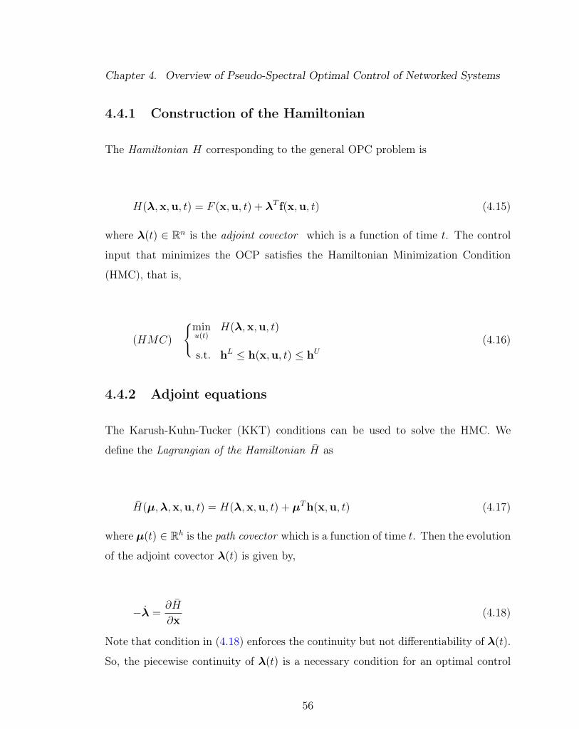
Chapter 4. Overview of Pseudo-Spectral Optimal Control of Networked Systems
4.4.1 Construction of the Hamiltonian
The Hamiltonian H corresponding to the general OPC problem is
H(λ,x,u, t) = F (x,u, t) + λT f(x,u, t) (4.15)
where λ(t) ∈ Rn is the adjoint covector which is a function of time t. The control
input that minimizes the OCP satisfies the Hamiltonian Minimization Condition
(HMC), that is,
(HMC)
minu(t)
H(λ,x,u, t)
s.t. hL ≤ h(x,u, t) ≤ hU(4.16)
4.4.2 Adjoint equations
The Karush-Kuhn-Tucker (KKT) conditions can be used to solve the HMC. We
define the Lagrangian of the Hamiltonian H as
H(µ,λ,x,u, t) = H(λ,x,u, t) + µTh(x,u, t) (4.17)
where µ(t) ∈ Rh is the path covector which is a function of time t. Then the evolution
of the adjoint covector λ(t) is given by,
−λ =∂H
∂x(4.18)
Note that condition in (4.18) enforces the continuity but not differentiability of λ(t).
So, the piecewise continuity of λ(t) is a necessary condition for an optimal control
56

Chapter 4. Overview of Pseudo-Spectral Optimal Control of Networked Systems
solution.
4.4.3 Minimization of the Hamiltonian
By the KKT condition, the minimization condition for the Hamiltonian yields
∂H
∂u= 0 (4.19)
with the complementary conditions for path constraints,
µi ≤ 0 if hi(x,u, t) = hLi
µi = 0 if hLi < hi(x,u, t) < hUi
µi ≥ 0 if hi(x,u, t) = hUi
µi unrestricted if hLi = hUi
(4.20)
If there are path constraints, then one of the necessary conditions is
µi(t)(hi − hLi )(hi − hUi ) = 0 (4.21)
Along with the minimization of the Hamiltonian, there is an endpoint minimization
condition (EMC) as well. The endpoint minimization problem is defined as
(EMC)
min E(x(t0),x(tf ), t0, tf )
s.t. eL ≤ e(x(t0),x(tf ), t0, tf ) ≤ eU(4.22)
57

Chapter 4. Overview of Pseudo-Spectral Optimal Control of Networked Systems
To solve the EMC by KKT, we define the endpoint Lagrangian E as
E(ν,x(t0),x(tf ), t0, tf ) =E(x(t0),x(tf ), t0, tf )
+ νT e(x(t0),x(tf ), t0, tf )(4.23)
where ν ∈ Re is the endpoint covector. Note that, ν is a constant vector. The
complementary conditions for event constraints are given by
νi ≤ 0 if ei(x(t0),x(tf ), t0, tf ) = eLi
νi = 0 if eLi < ei(x(t0),x(tf ), t0, tf ) < eUi
νi ≥ 0 if ei(x(t0),x(tf ), t0, tf ) = eUi
νi unrestricted if eLi = eUi
(4.24)
4.4.4 Hamiltonian Value condition
The lower Hamiltonian H is defined as the Hamiltonian evaluated at u(t) = u∗(t),
the solution to the HMC problem, i.e.,
H = minu∈U
H(λ,x,u, t) (4.25)
where U is the set of feasible control inputs, i.e., they satisfy all of the constraints
imposed by Eq. (4.1). The lower Hamiltonian must satisfy the endpoint value con-
ditions as a regular Hamiltonian
H(λ(t0),x(t0), t0) =∂E
∂t0
H(λ(tf ),x(tf ), tf ) = −∂E∂tf
(4.26)
which provides another necessary conditions to check for the optimal control solution.
58

Chapter 4. Overview of Pseudo-Spectral Optimal Control of Networked Systems
4.4.5 Time Evolution of the Hamiltonian
As the lower HamiltonianH is obtained from the evaluation of the Hamiltonian at the
u∗(t), x∗(t) and λ∗(t), where x∗(t) and λ∗(t) are the states and costates associated
with the optimal control solution u∗(t), H is a function of time t only. Thus the
evolution of the lower Hamiltonian H can be defined as
H =dHdt
=∂H
∂t(4.27)
If H in (4.15) does not depend explicitly on time, then another necessary condition
is
H = 0 or H = constant (4.28)
4.4.6 Transversality conditions
The endpoints of the adjoint covector λ(t) are related to the partial derivatives of
the endpoint Lagrangian E. The transversality conditions for the adjoint covector
λ(t) are
λ(t0) = − ∂E
∂x(t0)and λ(tf ) =
∂E
∂xf(4.29)
In chapter 6, we verify the necessary conditions for the optimal control problem
that we formulate and solve in that chapter.
59

Chapter 5
Optimal Regulation of Blood Glucose
Level in Type I Diabetes using
Insulin and Glucagon
5.1 Introduction
As our first implementation o the optimal control strategies, as discussed in chapter
1 to biological systems, we consider the Glucose-Insulin-Glucagon (GIG) model [57–
59, 115] which describes the response of the body to exogenously supplied insulin
and glucagon in patients affected by Type I diabetes. Common therapies for diabetes
involve the administration of exogenous insulin. Currently glucagon is not typically
included in therapies because it does not preserve its chemical properties at room
temperature and also because diabetic patients are still able to produce it.
The control of glucose levels in diabetic patients is an active field of research
[47–50, 60–64, 116–121]. The approval by the FDA of a simulator which replaces
in-vivo with in-silico therapy testing has greatly benefited this area of research. This
60

Chapter 5. Optimal Regulation of Blood Glucose Level
simulator implements a mathematical model, first proposed in [57] and updated in
[58, 59, 115], and provides an alternative to often slow, dangerous and expensive
human testing.
Typically, insulin is administered manually approximately half an hour before
each meal where the amount is determined from the current glucose level (measured
through a blood sugar test), the expected glucose intake, and the patient’s sensitivity
to insulin. In what follows we will refer to this as the standard therapy. In 1992 the
first insulin pumps were introduced to the market. They delivered both a consistent
basal amount of insulin and an insulin bolus determined by the patients based on
their glucose level. It was only in 2016 that the first autonomous system for glycemic
control was approved by the FDA. The system consists of an insulin pump, a sensor
that measures the blood glucose level continuously in time, and control software that
is able to regulate the insulin level in the blood without needing any input from the
patient.
Many control techniques have been proposed and tested to regulate blood glucose
levels using insulin pumps including PID (proportional–integral–derivative) control
[60–65], fuzzy logic control [117–119] and bio-inspired techniques [120] which do
not rely on a mathematical model. In [66] closed loop control has been used on a
so called “minimal model" [122–124]. In [47–51] a linear model predictive control
(MPC) has been used in a model with fixed structure but for which parameters
are constantly updated to adapt to the patient’s response. In [52] linear MPC has
been used in silico. In [53] MPC has been applied to a system linearized around
the operating points of a physically derived nonlinear model and in [67] multiple
model probabilistic predictive control has been used. In [54] MPC has been applied
together with a moving horizon estimation technique to a linear model. Most of the
models used when designing the above controllers are simplified versions of the FDA
approved model and all the control techniques considered only use insulin (but not
61

Chapter 5. Optimal Regulation of Blood Glucose Level
glucagon) as control input.
Because insulin delivered exogenously is not subject to normal physiological feed-
back regulation, hypoglycemia is common in patients with Type 1 diabetes who un-
dergo treatment [125]. For these patients it has been proposed that exogenous insulin
can be used to lower their blood glucose level and exogenous glucagon can be used
to prevent hypoglycemia [126, 127]. Currently, a commercial pump that delivers
both insulin and glucagon is not available, and the development of a two-hormones
artificial pancreas is still the subject of clinical research [128–136]. An outstand-
ing research question, which we address in this paper, is the determination of the
temporal dosages of both insulin and glucagon, in the case of the dual therapy.
Following the study in [137] which optimized multi-drug therapies for autophagy
regulation, here we seek to determine an optimal strategy for delivery of both insulin
and glucagon. We consider the combined effects of insulin and glucagon in regulating
blood glucose levels in patients with Type 1 diabetes, using the model in [58] and
nonlinear optimal control theory. Additionally, the objective function that we seek to
minimize is the Blood Glucose Index which is a well known tool to measure the risk
for a patient to enter either hyperglycemia or hypoglycemia. To design the optimal
control problem, we use the balance control technique of ref. [138], which introduces a
trade-off between the error allowed with respect to a state based cost (Blood Glucose
Index) and the control effort. Our goal is to evaluate the performance limits of a
control algorithm in the blood glucose problem, and to discuss the advantages of
the dual therapy compared to the single therapy. Note that even though we do not
attempt to design a closed-loop control strategy that works without the patient’s
intervention, the solution we propose can be adapted for that purpose.
From solving the optimal control problem for a family of objective functions
derived from the balance control paradigm, we observe the emergence of a pattern,
from which we propose a simple rule for the delivery of insulin and glucagon similar
62

Chapter 5. Optimal Regulation of Blood Glucose Level
to the standard therapy, but for the case that both insulin and glucagon are used.
While this therapy is suboptimal, we see that it still performs better than the optimal
solution with insulin alone.
Finally, we test the robustness of the optimal solution. While optimal control does
not guarantee robustness of the optimal solution with respect to model uncertainty
or parameter mismatches, we see that our proposed solution still performs well in
the presence of model parameter perturbations and variations affecting the time and
glucose intake of the meal.
5.2 Model and Parameters
We consider the model in [58, 59] which is a system of nonlinear ordinary differential
equations (ODEs). The equations are given in Eqs. (C.1)-(C.9) in the section C.1 in
Appendix C. We write the ODEs in Eqs. (C.1)-(C.9) in the form
x(t) = f(x(t),u(t), D(t),Θ)
G(t) = x1/VG(5.1)
where the state vector is x = [x1(t), x2(t), ..., x17(t)]T and t is the physical time
(in min). In Table 5.1 we tabulate all of the variables xi and their names. The
control input vector is u(t) = [uI(t), uG(t)]T , where uI(t) ≥ 0 is the exogenous
insulin infusion rate (in insulin Unit/min) and uG(t) ≥ 0 is the exogenous glucagon
infusion rate (mg/min). Both uI(t) and uG(t) are the external inputs to the system
in Eq. (5.1). The scalar quantity D(t) represents the exogenous glucose input, that
is, the glucose intake with a meal. The output of the system is the quantity G(t),
which measures the density of glucose in the blood, obtained as the ratio between
the plasma glucose and the distribution volume of glucose VG.
When uI(t) = 0, uG(t) = 0 and D(t) = 0, the model reaches (for physically
63

Chapter 5. Optimal Regulation of Blood Glucose Level
meaningful parameters) a steady state, also known as the basal condition of a patient.
The basal condition depends upon the parameters of the models Θ. We denote by
ΘGb a set of parameters for which the basal glucose level G is equal to Gb. The basal
levels for the other states are found according to Eqs. (C.11).
Table 5.1: Variables and their physical meaning
Variables Names Representing Units
x1 Gp Mass of glucose in plasma mg/kgx2 Gt Mass of glucose in tissue mg/kgx3 Il Mass of insulin in liver pmol/kgx4 Ip Mass of insulin in plasma pmol/kgx5 I ′ Mass of delayed in compartment 1 pmol/Lx6 XL Amount of delayed insulin action on EGP (Endogenous glucose production) pmol/Lx7 Qsto1 Amount of solid glucose in stomach mgx8 Qsto2 Amount of liquid glucose in stomach mgx9 Qgut Amount of glucose in intestine mgx10 X Amount of interstitial fluid pmol/Lx11 SRs
H Amount of static glucagon ng/L/minx12 H Amount plasma glucagon ng/Lx13 XH Amount of delayed glucagon action on EGP ng/Lx14 Isc1 Amount of nonmonomeric insulin in the subcutaneous space pmol/kgx15 Isc2 Amount of monomeric insulin pmol/kgx16 Hsc1 Amount of glucagon in the subcutaneous space 1 ng/Lx17 Hsc2 Amount of glucagon in the subcutaneous space 2 ng/L
5.3 Problem Formulation
We formulate a nonlinear optimal control problem with two control goals. The first
goal is to regulate the glucose at levels corresponding to low clinical risk of either
hyperglycemia or hypoglycemia during a time period over which a meal is consumed.
We assume that a meal is ingested at time t = τD, which we assume to be modeled as
a Dirac delta function D(t) = Dδ(t−τD). To evaluate the clinical risk of a particular
64

Chapter 5. Optimal Regulation of Blood Glucose Level
glycemic value, Kovatchev et al. [139, 140] proposed the Blood Glucose Index (BGI),
defined as
BGI (G(t)) = 10(1.509
((lnG(t))1.084 − 5.3811
))2,
where a small BGI value corresponds to low risk of either hyperglycemia or hypogly-
cemia. This metric also takes into account the fact that (i) the target blood glucose
range as defined by the Diabetes Control and Complications Trial [141] (between 70
and 180 mg/dL) is not symmetric about the center of the range and (ii) hypoglycemia
occurs at glucose levels closer to the basal level than hyperglycemia. The second goal
is to limit the overall usage of insulin and/or glucagon over the period [t0, tf ].
We formulate the optimization problem according to these two goals,
minu(t)
J =
∫ tf
t0
[αpBGI (G(t)) + αIupI(t) + αGu
pG(t)] dt, (5.2)
subject to the following constraints,
x(t) = f(x(t),u(t), Dδ(t− τD),ΘGb), u(t) = [uI(t) uG(t)]T (5.3a)
GL < G(t) < GU (5.3b)
uLI ≤ uI(t) ≤ uUI (5.3c)
0 ≤ uG(t) ≤ uUG (5.3d)
0 ≤∫ tft0uI(t)dt ≤ φUI (5.3e)
0 ≤∫ tft0uG(t)dt ≤ φUG (5.3f)
x(t0) = x (5.3g)
In Eqs. (5.2) and (5.3), the insulin infusion rate uI(t) and the glucagon infusion rate
uG(t) are the two control inputs. The three coefficients αp, αI and αG in Eq. (5.2)
are tunable factors through which we may vary the weight associated with each of
65

Chapter 5. Optimal Regulation of Blood Glucose Level
the three terms in the cost function J . The first coefficient, αp is dimensionless while
the units of αI and αG are (U/min)−p and (mg/min)−p, respectively. Note that by
setting uG = 0 in Eq. (5.3d), we have an optimal control problem in terms of insulin
only.
The first term in the objective function (5.2) defines a regulation problem, i.e.,
we try to maintain the glucose at low risk levels. The second and third terms in the
cost function are chosen to avoid using excess insulin or glucagon. For p = 1 in Eq.
(5.2), the second and third terms define a ‘minimum fuel’ problem, thus we call the
optimization problem ReMF (Regulation and Minimum Fuel). In this case, we expect
the optimal solution to consist of pulsatile inputs u∗I(t) and u∗G(t) [110, 142]. For
p = 2, the second and third term inside the cost function define a ‘minimum energy’
problem, thus we call the optimization problem ReME (Regulation and Minimum
Energy). In this case, we expect the optimal control inputs u∗I(t) and u∗G(t) to be
continuous. The set of equations in (5.3a) coincide with the ODEs in Eqs. (C.1)-
(C.9)of the supplemental information. In Eq. (5.3b) GL and GU are the lower and
upper bounds for G(t), they can be set in order to avoid undesired hypoglycemic
or hyperglycemic states. In Eqs. (5.3c) and (5.3d) uUI and uUG are upper bounds for
the insulin and glucagon delivery rates, respectively. These constraints are set by
the maximum infusion rates allowed by the insulin pump. In Eq. (5.3c) uLI ≥ 0 is
the lower bound for uI(t), i.e., a minimum insulin delivery rate that can be used to
set a basal insulin infusion rate to counteract endogenous glucose production [143].
Finally, in Eqs. ((5.3e), (5.3f)), φUI and φUG set limits to the total limits of insulin and
glucagon that can be delivered over the time period [t0, tf ]. The initial condition x
in Eq. (5.3g) defines the patient’s condition before administration of the therapy. In
the Results section, we discuss how we choose the bounds on G(t), uI(t), uG(t), φI ,
φG, the control time period [t0, tf ] and the initial condition x.
Our goal is to find an optimal solution which satisfies the constraints in Eq. (5.3)
66

Chapter 5. Optimal Regulation of Blood Glucose Level
and minimizes the objective function (5.2). Note that the BGI only depends upon
G(t): we are making no attempt to control the states of the system, only its output.
In the literature, such an approach is often referred to as target control [95, 110].
5.4 Method
The equations (5.2) and (5.3) together form a constrained optimal control problem,
which can generally be written as Eq. (4.1). We have used PSOPT [112], an open-
source PSOC library, to perform the above PSOC discretization procedure. The
NLP in (4.8) can be solved with a number of different techniques, but here we use
an interior point algorithm [56] as implemented in the open-source software Ipopt
[113].
5.5 Results
We now describe in more detail the optimal control problem in Eqs. (5.2) and (5.3)
by setting the constraint and parameter values. In Fig. 5.1(A) we plot the function
BGI(G) versus the glucose G. The minimum BGI (G) occurs at G = Gd = 112.51
mg/dL, which corresponds to a clinical target set for the glucose level [141]. Based
on the data in [144], the average fasting plasma glucose level of patients with type
I diabetes is Gb = 130 (mg/dL). Thus, we set the the basal glucose level Gb = 130
(mg/dL). The parameters ΘGb are set so that the steady state glucose is 130 (mg/dL)
in the absence of a meal and of exogenously supplied insulin, i.e., we compute Θ130.
We set the upper and lower bounds for the glucose level, GL and GU in Eq.
(5.3b), to satisfy the target blood glucose range, 90 ≤ G(t) ≤ 180 [141]. The control
time period is [t0, tf ] = [0, 300] minutes, and we assume that a meal with 70 grams
67

Chapter 5. Optimal Regulation of Blood Glucose Level
50 2000
10
20
Gd
A)
Glucose (G(t)) (mg/dL)
BGI(G
(t))
0 500 1,000
110
120
130
B)
Time (t) (min)
Glucose
(mg/dL)
ub = 0.00 (U/min) n
ub = 0.0012 (U/min)
ub = 0.0024 (U/min)
Gd = 112.51 (mg/dL)
Figure 5.1: (A) The Blood Glucose Index (BGI(G(t))) as a function of the bloodglucose G(t). The function is minimized at G(t) = Gd = 112.51 (mg/dL). (B) Theresponse of glucose (G(t)) to different time-constant basal insulin infusion rates inthe absence of a meal. We see that as ub increases, the glucose is further downregulated.
of glucose is consumed at time t = 60 min (i.e. D(t) = 70δ(t− 60)).
We consider a situation in which the patient’s glucose level is partially controlled
by providing a constant but low insulin infusion rate ub > 0 (which is common for
patients who use an insulin pump) [143] and serves to compensate for the endogenous
glucose production. In figure 5.1B we show glucose response G(t) for different values
of constant ub in the absence of a meal. We observe that for ub = 0.0024 (U/min),
G(t) converges to the desired glucose level Gd. We thus set the lower bound of
uI(t) in Eq. (5.3c), uLI = ub, while its upper bound is set to uUI = 15 (in U/min),
the maximum insulin flow allowed in commercial pumps [145]. In the absence of
commercially available glucagon pumps, we will assume that a pump mechanically
similar to an insulin pump is used to deliver glucagon. Since the maximum flow
rate for an insulin pump is 0.15 mL/min (1 mL of insulin solution contains 100 U of
insulin), and normally 1 mg of glucagon is diluted in 1 mL of solution, the maximum
glucagon flow rate in Eq. (5.3d) is set to uUG = 0.15 mg/min.
The amount of insulin administered in a bolus to a patient with a basal glucose
level lower than 150 mg/dL normally ranges between 0.12 and 0.2 U/kg [146]. As
68

Chapter 5. Optimal Regulation of Blood Glucose Level
the body mass of the in-silico patient we consider is 78 kg, we set φUI = 16 U in
Eq. (5.3e). The maximum total amount of glucagon administered in one shot to
a patient who is in a hypoglycemic state is 1 mg, and a second identical shot can
be administered after thirty minutes. We thus choose the maximum total amount
of glucagon used (as defined in Eq. (5.3f)) throughout the five hour therapy to be
φUG = 1mg.
The choice of the initial condition x in Eq. (5.3g) is critical. We select the
initial condition so that the solution of our optimal control problem only attempts
to regulate glucose in response to a meal. In the results presented we have set the
initial condition equal to the values of the states when uI(t) = ub after a period
of fasting (the final point of the blue curve in Fig. 5.1(B). If we were to select any
alternative initial condition then the solution to the optimal control problem would
try to ‘correct’ the initial condition as well, making comparisons between solutions
difficult.
Once the parameters, bounds, the control time period and the initial condition
are set, we solve the nonlinear optimal control problem using PSOPT . We first
solve the optimal control problem without glucagon (i.e. uUG = 0), and then we solve
the optimal control problem using both insulin and glucagon.
To evaluate the effectiveness of the obtained results, we introduce the following
measures.
• The cumulative insulin rI(t) and cumulative glucagon rG(t) used up to time t,
rI(t) =
∫ t
t0
uI(τ)dτ, rG(t) =
∫ t
t0
uG(τ)dτ.
• The total amount of insulin φI = rI(tf ) and the total amount of glucagon
φG = rG(tf ) used up to final time tf .
69

Chapter 5. Optimal Regulation of Blood Glucose Level
• The integral of BGI over the entire time period [t0, tf ],
∆ =
∫ tf
t0
BGI(G(t))dt.
where a large ∆ indicates that the patient is at higher risk of either hypergly-
cemia or hypoglycemia for a prolonged period of time.
• The maximum and minimum values attained by the blood glucose level over
the entire time period [t0, tf ],
Gmax = maxt∈[t0,tf ]
G(t), Gmin = mint∈[t0,tf ]
G(t),
which measure the risk for either hyperglicemia or an hypoglicemia [140, 147],
respectively.
5.5.1 Insulin as Control Input
In this section we use only insulin as control input, i.e., we set uG = 0 in Eq. (5.3a).
As the orders of magnitude of the terms BGI and upI in the objective function are
different, it is important to find the appropriate values of the scaling factors αp and
αI . In what follows, we use a Pareto-front analysis to determine these values. We
first rewrite the objective function as
J =
∫ tf
t0
[εBGI(G(t)) + upI ] dt (5.4)
where ε = αp/αI . In Figs. 5.2(A–D) we plot ∆, Gmin, Gmax and φI as functions
of the coefficient ε. By looking at these plots, we see that the four measures can
be divided into two groups. On the one hand, ∆ and Gmax (panels (A) and (C )),
improve (decrease) as ε increases, with a sharp transition around ε = 10 for the
ReMF problem and around ε = 103 for the ReME problem. On the other hand,
Gmin and φI (panels (B) and (D), behave in the opposite way, i.e., they improve
70

Chapter 5. Optimal Regulation of Blood Glucose Level
10−2 100 102 104
102
103
A)
ε
∆
10−2 100 102 10490
95
100
105
110
B)
ε
Gmin
10−2 100 102 104120
140
160
180
C )
ε
Gmax
10−2 100 102 104
6
8
10
D)
ε
φI
6 8 10101
102
103
E )
φI
∆
ReMF (P = 1)ReME (P = 2)
Figure 5.2: Performance of the optimal control solution as a function of ε. Large(small) values of ε correspond to a large (small) weight associated with the BGIindex in the objective function, compared to the weight for insulin expenditure. Thefirst four plots show our metrics as functions of the objective function coefficients:(A) ∆ vs. ε, (B) Gmin vs. ε, (C ) Gmax vs. ε, and (D) φI vs. ε. (E ) We also projectthe Pareto front into the ∆ - φI plane. We see a clear trade-off between ∆ and φIas we vary ε. By increasing ε we can decrease the values of ∆ and Gmax. However,the values of ∆ and Gmax do not further decrease for ε larger than 10 for the ReMFproblem (p = 1) and the value of ∆ does not further decrease for ε larger than 103
for the ReME problem (p = 2). We choose ε = 10 for p = 1 and ε = 103 for p = 2,which are indicated by dashed circles in the figure, for the remaining simulations.
(insulin decreases and the minimum glucose level increases) as ε decreases, again
with a sharp transition around ε = 10 for the ReMF problem and around ε = 103
for the ReME problem. Because the four curves in Figs. 5.2(A–D) are monotone, all
the points are Pareto-efficient, i.e., it is not possible to improve one objective (e.g.
∆) without worsening the other one (e.g. φI). We notice that past a certain value of
ε (10 in the ReMF case, 103 in the ReME case) ∆ and Gmax do not further decrease
and Gmin and φI remain unchanged. We choose as weights αp = 10 and αI = 1
for p = 1, while we choose αp = 103 and αI = 1 for p = 2 (these are highlighted
71

Chapter 5. Optimal Regulation of Blood Glucose Level
by dashed circles in Fig. 5.2). The reason for these choices (for both values of p) is
that these values yield φI ∼ 10 units, which is equal to two thirds of the maximum
amount of insulin that can be supplied (φUI ), and Gmin ∼ 93mg/dL, which is far from
the hypoglycemic risk region.
In Fig. 5.2(E ), we plot a projection of the Pareto front in the ∆ and φI plane.
Looking at this plot, the trade-off between ∆ and φI is evident; if the total amount of
insulin expenditure increases, ∆ decreases and vice-versa. The ReMF and the ReME
therapies can also be compared in Fig. 5.2(E ). The ReMF Pareto front dominates
the ReME one (both ∆ and φI are lower on the blue curve (p = 1) compared to the
magenta curve (p = 2)). This indicates that a shot of insulin (the optimal solution of
a ReMF problem is typically a pulsatile function) performs slightly better in terms
of ∆ than a therapy in which the insulin is delivered over a longer period of time
while using less insulin.
Figure 5.3 shows the results of the optimal control problem for the selected values
of αp and αI . The blue and magenta curves are the optimal solutions of the ReMF and
of the ReME problem, respectively. The orange curve corresponds to the case that
10 U of insulin are injected 30 minutes before the time of the meal, i.e., the standard
therapy. We observe that for P = 1 the optimal insulin infusion rate is pulsatile
with a pulse appearing at t ∼ 20 minutes, which is 40 minutes before the time of
the meal. We obtained qualitatively similar results for different choices of the model
parameters, with the pulse typically appearing at a time in the interval t ∈ [20, 30]
minutes. It is noteworthy that the optimal solution is close to the standard insulin
based therapy for glucose regulation in diabetics. The optimal insulin infusion rate is
continuous when we solve the ReME problem, also shown in the inset of Fig. 5.3(B).
Note that the ReMF and ReME therapies perform very similarly with respect to
glucose as the peak insulin infusion rate occurs at approximately the same time and
the total amount of insulin administered is nearly equal.
72

Chapter 5. Optimal Regulation of Blood Glucose Level
5.5.2 Insulin and Glucagon as Control Inputs
In the previous section we tuned the weights αp and αI inside the objective function
(5.2). We now consider the case that uG > 0 and we tune αG, the weight associated
with the glucagon expenditure in the objective function (5.2), by keeping αp = 10,
αI = 1 for P = 1 and αp = 103, αI = 1 for p = 2 , as previously determined.
0 50 100 150 200 250 300
90
110
130
A)
Time (t) (min)
Glucose
(mg/dL)
0 50 100 150 200 250 3000
5
10
15
B)
Time (t) (min)
Insulininfusion
rate
(U/m
in)
0 50 100 150 200 250 3000
5
10
C )
Time (t) (min)
Cumulative
Insulinr I(t)(U
)
0 20 40 60 80
0
0.5
1
ReMF ReME Standard(P = 1) (P = 2) Therapy
∆ 105.17 109.27 153.83
Gmin (mg/dL) 92.85 92.43 88.10
Gmax (mg/dL) 130.65 130.62 121.72
φI (U) 10.07 10.10 10
Figure 5.3: (A) The time evolution of glucose G(t) (in mg/dL). The blue curve cor-responds to the pulsatile optimal insulin supply rate uI(t) (shown in (B) obtained bysolving the ReMF problem. The magenta curve corresponds to the continuous op-timal insulin supply rate uI(t) (shown in (B) obtained by solving the ReME problem.The orange curve is the time evolution of G(t) corresponding to the standard therapy(10 U of insulin injected 30 minutes before the time of the meal). (B) Time evolutionof the optimal insulin infusion rates uI(t) (in U/min). Color code is consistent with(A). (C ) Cumulative insulin supply rI(t) (in U) as a function of t.
73

Chapter 5. Optimal Regulation of Blood Glucose Level
10−3 100 1030
50
100
150
A)
αG
∆
10−3 100 10390
100
110
B)
αG
Gmin
10−3 100 103
120
130
140
C )
αG
Gmax
0 0.5 1
10
12
14
16
D)
φG
φI
0 0.5 10
50
100
150
E )
φG
∆
ReMF (P = 1)
ReME (P = 2)
Figure 5.4: Performance of the optimal control solution as a function of αG. (emphA)∆ vs. αG. (B) Gmin vs. αG. (C ) Gmax vs. αG. (D) φI vs. φG. (E ) ∆ vs. φG. Weselect αG = 10−2 for both of the REMF and REME problems, which are indicatedby dashed circles in the figure.
In Fig. 5.4(A), 5.4(B) and 5.4(C ), we plot the optimal ∆, Gmin and Gmax as
functions of the parameter αG, respectively. A large value of αG indicates that we are
placing a large weight on the expenditure of glucagon within the objective function
(5.2), i.e., the larger the value of αG, the less glucagon we use. By looking at Fig.
5.4(A), we observe that the values of ∆ decrease as αG decreases, i.e. we can obtain
lower (improved) values of ∆ if we allow for a larger expenditure of glucagon. We
note that past a certain value of αG (10−2 in the both the ReMF and ReME problems)
no further reduction in ∆ is observed. As in the previous case, the maximum glucose
level Gmax, shown in Fig. 5.4(C ), improves (decreases) when ∆ improves (decreases).
Interestingly, different from the previous case, also the minimum glucose level Gmin
(Fig. 5.4(C ) improves (increases) with ∆ and Gmax: this is a consequence of the fact
that we are using both insulin and glucagon as control inputs, which enables us to
avoid both hypoglycemia and hyperglycemia.
74

Chapter 5. Optimal Regulation of Blood Glucose Level
In Fig. 5.4(D) we plot the projection of the Pareto front in the (φI , φG) plane.
By looking at the figure, φI and φG appear to be positively correlated and related
by an approximately linear relation. While the timing of administration of insulin
and glucagon is different, we see that overall the more insulin is used in the optimal
solution, the more glucagon is used as well. This is because the two hormones have
opposite effects in the regulation problem and thus they work so as to balance each
other. This is also consistent with the observation that with the dual therapy (insulin
and glucagon) it becomes possible to simultaneously improve ∆, Gmin, and Gmax.
From the data in Fig. 5.4(D) we derive the following approximate linear relationship
between φG and φI ,
φG(φI) = 0.1596φI − 1.5796 (5.5)
Obviously, glucagon should be used only when φG(φI) > 0.
Panel 5.4(E ) shows a projection of the Pareto front on the (φG,∆) plane. We see
again that the ReMF front dominates the ReME one, i.e., a pulsatile therapy gives
better results than a continuous therapy in terms of ∆ and also uses lower amounts
of the two hormones (smaller φG, and thus smaller φI due to the positive correlation
found in Fig. 5.4(D).
The Pareto front is monotonically decreasing in Fig. 5.4(E ) which indicates a
trade-off between the total amount of hormones used and the achievable glucose
control performance. We choose the value of αG for which the ratio between the
increase in ∆ and the decrease in φG is minimized, i.e. αG = 10−2 for both ReMF
and ReME problems, which are indicated by dashed circles in the figure.
Figures 5.5(A) and 5.5(B) show the results of the optimal control problem for
αp = 10, αI = 1 and αG = 10−2 when P = 1; and αp = 103, αI = 1 and αG = 10−2
when p = 2. In Fig. 5.5(A) we plot the time evolution of glucose G(t) for the different
optimal solutions. The blue curve corresponds to the solution of the ReMF problem
75

Chapter 5. Optimal Regulation of Blood Glucose Level
when only insulin is used (the blue curve in Fig. 5.3(A). The red and green curves
correspond to the solution of the ReMF and the ReME problems for the dual therapy.
We observe that G(t) reaches the desired level Gd faster if we use both insulin and
glucagon as control inputs, compared to the case that only insulin is used. We also
see that in this case both Gmax decreases and Gmin increases. We therefore conclude
that the therapy with both insulin and glucagon performs better than the therapy
with only insulin, as the risks for both hypoglycemia and hyperglycemia are reduced
and glucose fluctuations are suppressed.
In Fig. 5.5(B) we plot the optimal insulin infusion rates and in Fig. 5.5(C ) we
plot the cumulative insulin supply rI(t) as a function of time t. We observe that for
the ReMF problem, the pulse in insulin appears at t = 32 minutes in the case that
both insulin and glucagon are used (28 minutes before the meal), whereas the pulse
appears at t = 20 minutes when only insulin is used. From Fig. 5.5(D), we see that,
for the ReMF problem, the glucagon delivery function is pulsatile with a main pulse
appearing at t = 145 min (one hour and 25 minutes after the meal) and a secondary
pulse appearing at t = 203. The dual therapy shows a noticeable difference between
the ReMF solution and the ReME solution. As expected, the solutions of the ReME
problem are continuous. The glucose response to the ReME therapy is better than
the glucose response to the ReMF solution. Specifically, the green curve has smaller
oscillations (in panel (A) at the cost of small increases in the total amounts of used
insulin and glucagon (compare panels (C ) and (E )).
Based on the results in Fig. 5.5, we propose a possible ad-hoc dual therapy to be
used as an alternative to the standard therapy. Rather than administering insulin
half an hour before the meal (standard therapy), better glucose regulation can be
achieved with a slightly larger insulin injection half an hour before a meal followed by
a glucagon injection one hour and thirty minutes after a meal. The insulin injection
of the ad-hoc dual therapy is 25% larger than the one used in the standard therapy,
76

Chapter 5. Optimal Regulation of Blood Glucose Level
which is consistent with the relation between φI for the monotherapy ReMF optimal
solution and the one used in the dual therapy.
In Fig. 5.6 we present a comparison between the glucose response to the standard
insulin base therapy (orange curve) and the proposed ad-hoc dual therapy (cyan
curve) for the case of a meal with 70 grams of glucose (for the particular patient
considered this corresponds to 10 units of insulin half an hour before the meal) and
the proposed ad-hoc dual therapy (which consists of 12.43 units of insulin thirty
minutes before the meal and 0.40 mg of glucagon one hour and thirty minutes after
the meal). We observe that the ad-hoc dual therapy performs better in terms of all
of the proposed measures (∆, Gmin, Gmax, φI and φG) as opposed to the standard
insulin based therapy.
5.6 Robustness Analysis
We now analyze the robustness of the optimal control therapies we have proposed
with respect to model parameter mismatches, which is a fundamental step for imple-
mentation of model based control. We consider two different types of mismatches.
The first type accounts for variability in the patient’s behavior, in terms of both the
time of the meal τD and the amount of glucose intake D. The second type accounts
for deviations in the parameter estimation, as well as the temporal variability of the
parameters that a patient may experience during the day [59].
5.6.1 Robustness Against Variability of the Meal Time and
Glucose Intake
In this section we analyze the robustness of the optimal ReMF therapies (both mono-
therapy and dual therapy) with respect to the two “control" parameters the patient
77

Chapter 5. Optimal Regulation of Blood Glucose Level
has. The first one is the variation in the meal time, (τD − τD) (min), where τD is
the time of a meal and τD is the time of a meal we assumed in order to compute the
optimal therapies. The second one is the variation of glucose in the meal, (D −D),
where D is the glucose intake in a meal and D is the glucose intake we assumed to
compute the optimal therapies. We consider variations in the meal time τD in the
interval [30, 90] min and variations of the glucose intake D in the interval [40, 100] g.
The results of this study are illustrated in Fig. 5.7. Figure 5.7 provides a visual
assessment of the quality of the optimal therapies in terms of the three proposed
measures ∆, Gmax and Gmin (the over-bar stands for evaluation at the perturbed
parameter values (τD, D)). The color in Fig. 5.7 varies according to the control
performance from green (good) to red (dangerous). In the upper panels (A–C )
we consider the optimal ReMF monotherapy, while in the lower panels (D-F ) we
consider the optimal ReMF dual thearpy. Cross symbols indicate the application of
the optimal control therapies under ideal condition, i.e., when τD = τD and D = D.
The black curves labeled by 180, 90 and 70 in Figs. 5.7(B), 5.7(C ), 5.7(D), 5.7(E )
are the curve level plots for Gmax = GU , Gmin = GL and Gmin = 70, respectively.
The black curves labeled by 180 in Figs. 5.7(B), and 5.7(E ), are the curve level plots
for Gmax = GU .
We see from Figs. 5.7(A) and 5.7(D) that the optimal therapies for the ReMF
problem (using only insulin or both insulin and glucagon) are robust with respect
to variations in the control parameters: ∆ remains well bounded in most of the
considered parameter space. In particular we see from Figs. 5.7(B) and 5.7(E ) that
the proposed optimal therapies are robust against hyperglicemic events: for example,
even if D exceeds D by 50% and τD exceeds τD by 30 minutes, the patient will not
enter the hyperglycemic regime (Gmax > 300). Figures 5.7(C ) and 5.7(F ) reveal
that the proposed therapies suffer from a certain lack of robustness with respect to
hypoglycemic events (Gmin < 70), the most dangerous ones. The dangerous cases
78

Chapter 5. Optimal Regulation of Blood Glucose Level
are, however, confined to extreme situations in which D < 0.5D and τD = τD + 30
minutes. Figures 5.7(C ) and 5.7(F ) show also that the optimal therapy for the
ReMF problem with both insulin and glucagon is more robust (larger green region
and smaller yellow region) than the optimal therapy for ReMF problem with only
insulin (smaller green region and larger yellow region): thus the use of glucagon
alleviates the risk of severe, life-threatening hypoglycemia.
We obtain qualitatively similar results when performing the same analysis for the
other therapies we proposed (the ReME therapies and the ad-hoc dual therapy).
5.6.2 Robustness to Parameter Mismatches
We consider perturbation of the model parameters up to 20% of their nominal values,
Θi = Θi(1 + ϕ), (5.6)
where ϕ is a random number from a normal distribution N (0, 0.0672), Θi is a nom-
inal parameter for a given patient with basal glucose level Gb and Θi represents the
associated perturbed parameter. We then apply the optimal insulin and glucagon
dosing, calculated for the unperturbed system, to 100 perturbed systems. This is
analogous to testing the computed optimal control therapy on a specific patient, but
the patient’s parameters may vary due to imperfect knowledge or due to the para-
meter variability throughout the day. The results of this study are illustrated with a
Control Variability Grid Analysis (CVGA), see Fig. 5.8. The CVGA provides a sim-
ultaneous visual and numerical assessment of the overall performance of the glycemic
control strategies in terms of the achieved minimum/maximum glucose values in the
space of parameters mismatches. In Fig. 5.8, points in the light green region indicate
accurate blood glucose control while points in the dark green regions indicate the
patient is not immediately at risk of either hypoglycemia or hyperglycemia. Points
79

Chapter 5. Optimal Regulation of Blood Glucose Level
in the top two yellow/orange regions indicate an elevated risk of hyperglycemia and
points in the the right two yellow/orange regions indicate an elevated risk of hy-
poglycemia. Finally, points in the red corner region indicate an elevated risk of both
hyperglycemia and hypoglycemia. Each point reported in the figure is a plot of Gmax
vs. Gmin. Here, the black dots correspond to the glucose response when a certain
therapy is applied to a system with perturbed parameters. Cross symbols indicate
application of the optimal control therapies to the unperturbed systems.
For the of monotherapy (ReMF in Fig. 5.8A and ReME in Fig. 5.8B) we find
that the control is 67% and 61% accurate, respectively. For the dual therapy case
(ReMF in Fig. 5.8(C ) and ReME in Fig. 5.8(D) we find the control is more ac-
curate than for the case of monotherapy, 92% and 94% accurate, respectively. The
least robust control is obtained with the standard therapy (shown in Fig. 5.8(E ),
attaining only 37% accuracy. Note that the optimal dual therapies (Figs. 5.8(C ) and
5.8(D)) are not only more robust than the optimal insulin therapies (Figs. 5.8(A)
and 5.8(B)), but also than the standard therapy (Fig. 5.8(E )). We also see that the
ad hoc therapy (Fig. 5.8(E )) is more robust than the standard therapy (Fig. 5.8(E )).
5.7 Discussion
In this paper we have used the Glucose-Insulin-Glucagon mathematical model pro-
posed in [58, 59, 115], which describes how the body responds to exogenously supplied
insulin and glucagon in patients affected by Type I diabetes and designed an optimal
dosing schedule of either insulin or insulin and glucagon together to regulate the
blood glucose index (BGI), while limiting the total amount of insulin and glucagon
administered. The numerical optimal control software PSOPT has been used to
solve this optimal control problem. While the numerical solution requires knowledge
of the set of model parameters, which are patient specific, the solutions we obtain
80

Chapter 5. Optimal Regulation of Blood Glucose Level
provide insight into the best possible glucose regulation with insulin or with insulin
and glucagon together. Our approach is in agreement with the results of references
[148–150], in which simplified models are used to analytically establish general the-
oretical properties and control limitations for the glucose regulation problem.
Two distinct regulation problems have been considered: the minimum fuel prob-
lem (ReMF) which yields pulsatile (shot-like) type solutions and the minimum energy
problem (ReME) which yields longer periods of time over which insulin is admin-
istered but with smaller delivery rates. This has allowed us to compare standard
therapies which typically consist in shots of insulin with therapies in which insulin
is delivered continuously. In [151, 152] it has been proven that the optimal control is
pulsatile when the aim of the control is to minimize the variation in the maximum
and minimum output response, the system is positive (like the one we are consid-
ering) and the disturbance (the meal, in our case) is pulsatile. Our work indicates
that pulsatile control is still a good choice when more complex objective functions
are chosen. Moreover, a pulsatile control appears to be optimal for alternative more
realistic models of the meal (for example, a meal that is consumed over a window
of 15 minutes). We also see that a continuous hormones delivery can achieve better
results in the case of the dual therapy, thus pointing out the importance of developing
a commercial pump able to deliver both insulin and glucagon.
For both the ReMF and ReME problems, we compute the optimal hormone
dosing schedules when only insulin is available and when both insulin and glucagon
are available. The solution of the insulin only ReMF problem, astoundingly, is nearly
equal to the standard method of insulin based glucose regulation. Similarly, the
solution of the ReMF problem when insulin and glucagon are used is also pulsatile,
except that the amount of insulin administered is larger and the administration time
is closer to the time of the meal, while the glucagon is mostly delivered in a shot
about an hour and thirty minutes after the meal.
81

Chapter 5. Optimal Regulation of Blood Glucose Level
The solution for the ReME problem when insulin only is available as well as
when both insulin and glucagon are available is different from the ReMF solution
in that, rather than being pulsatile, insulin and possibly glucagon are delivered at
a slower rate over longer periods of time. Nonetheless, the total amount of insulin
and possibly glucagon is about the same, and the peak of the longer delivery time
occurs approximately at the same time of the shot according to the solution of the
ReMF problem. The obtained glucose profiles for the optimal ReMF and ReME
problem solutions do not differ too much from each other: taken together, these
results indicate that the amounts of insulin and glucagon, and the peak times of
delivery, are the most important factors to determine when computing the optimal
solutions.
Based on the above results, we have proposed the following ad hoc therapy when
insulin and glucagon are used in combination: Administer a shot of insulin (with
25% more insulin than the amount required by the standard therapy based on the
planned meal) 30 minutes before eating. Administer a shot of glucagon of an amount
specified by Eq. (5.5) one hour and thirty minutes after completing the meal. This
therapy should be used with caution as the amount of insulin injected can lead to
hypoglycemia if the shot of glucagon is not administered as well.
All optimal dosing schedules we computed were tested for robustness with re-
spect to variations in the meal timing and size and with respect to variability of
the parameters. The therapies we proposed typically maintain the patient in the
healthy region even under variable conditions and patient behavior. Note, however,
that the proposed therapies are open-loop, thus cannot compensate for unexpected
behavior that can arise due to modeling simplifications (e.g. we do not consider
how physical activity influences the blood glucose levels [153, 154]), measurement
noise or bias. A step towards the real application of our methodology is a real-time
closed-loop strategy; this is possible, since the typical time needed to compute an
82

Chapter 5. Optimal Regulation of Blood Glucose Level
optimal solution on a standard laptop (i7-8550U CPU with 16GB RAM) is around 2
minutes. Another main limitation of our study is that real life constraints and long
term physiological effects may make a therapy based on exogenous administration of
both insulin and glucagon impractical.
Our optimal control strategies require knowledge of the meal time and meal gluc-
ose amount. This is somewhat undesirable, as recent advances in diabetes therapy
have moved towards devices that do not require the user to provide information about
the meals. Our results emphasize the importance of incorporating information about
the meals in the dosing schedules and indicate a potential benefit of providing the
pump with the ability to interpret the patient’s behavior. The results from this
chapter have been published in [155].
83

Chapter 5. Optimal Regulation of Blood Glucose Level
0 50 100 150 200 250 30090
110
130
150
A)
Time (t) (min)
Glucose
(mg/dL)
0 50 100 150 200 250 300
0
5
10
15
B)
Time (t) (min)
Insulininfusion
rate
(U/m
in)
0 50 100 150 200 250 300
0
5
10
15
C )
Time (t) (min)
Cumulative
Insulinr I(t)(U
)
0 50 100 150 200 250 3000
0.1
0.2
0.3
D)
Time (t) (min)
Glucagoninfusion
rate
(mg/min)
0 50 100 150 200 250 3000
0.5
1E )
Time (t) (min)
Cumulative
glucagonr G
(t)(m
g)
0 100 200 3000
0.1
0.2
0 100 200 300
0
0.005
0.01
ReMF ReME ReMF(P = 1) (P = 2) (P = 1)
∆ 21.96 14.66 105.17
Gmin (mg/dL) 99 100.43 92.85
Gmax (mg/dL) 123 120.15 130.65
φI (U) 12.43 13.29 10.07
φG (mg) 0.37 0.53
Figure 5.5: (A) Time evolution of glucose G(t) (in mg/dL). The blue curve corres-ponds to uI(t) obtained by solving the ReMF problem . The red curve correspondsto uI(t) and uG(t) obtained by solving the ReMF problem using the dual therapy.The green curve corresponds to uI(t) and uG(t) obtained by solving the ReME prob-lem using the dual therapy. (B) Time evolution of the insulin infusion rate uI(t) (inmg/dL). Color code is consistent with (A). (C ) The cumulative insulin supply rI(t)as a function of time t. (D) Time evolution of the glucagon infusion rate uG(t) (inmg/dL). (E ) The cumulative glucose supply rG(t) as a function of time t.
84

Chapter 5. Optimal Regulation of Blood Glucose Level
0 50 100 150 200 250 30080
100
120
Time (t) (min)
Glucose
(mg/dL)
Standard ad-hocTherapy Therapy
∆ 153.83 62.26
Gmin (mg/dL) 88.10 96.82
Gmax (mg/dL) 121.72 112.59
φI (U) 10 12.43
φG (U) 0.40
Figure 5.6: Comparison between the glucose response to the standard insulin basetherapy (orange curve) and the proposed ad-hoc dual therapy (cyan curve).
85

Chapter 5. Optimal Regulation of Blood Glucose Level
A)
-30 -20 -10 0 10 20 30-30
-20
-10
0
10
20
30
(D−D
)(g
)
5
10
15
∆/∆
180
B)
-30 -20 -10 0 10 20 30-30
-20
-10
0
10
20
30
150
200
Gmax
90
90
70
C )
-30 -20 -10 0 10 20 30-30
-20
-10
0
10
20
30
60
80
100
Gmin
D)
-30 -20 -10 0 10 20 30-30
-20
-10
0
10
20
30
(τD − τD) (min)
(D−D
)(g
)
20
40
60
80
∆/∆180
180
E )
-30 -20 -10 0 10 20 30-30
-20
-10
0
10
20
30
(τD − τD) (min)
150
200
Gmax
90
90
70
F )
-30 -20 -10 0 10 20 30-30
-20
-10
0
10
20
30
(τD − τD) (min)
60
80
100
Gmin
Figure 5.7: Robustness of the optimal control solution against variations in themeal timing and the amount of glucose in the meal. (A)–(C ) show the resultsobtained for the ReNF problem (P = 1) with only insulin provided, (D)-(F ) ReMF(P = 1) problem with both insulin and glucagon provided. Cross symbols indicatethe application of the optimal control therapies for D = D and τD = τD. Theblue cross symbols correspond to the optimal therapies for the ReMF problem withonly insulin. The red cross symbols correspond to the optimal therapies for theReMF problem with both insulin and glucagon. (A) and (D) are plots of ∆/∆ inthe control parameters space (τD, D). (B) and (E ) are the plots of Gmax in thecontrol parameters space (τD, D). (C ) and (F ) are the plots of Gmin in the controlparameters space (τD, D).
86

Chapter 5. Optimal Regulation of Blood Glucose Level
> 110 90 70 50< 110
180
300
400
A)
Gmax
> 110 90 70 50< 110
180
300
400
B)
> 110 90 70 50< 110
180
300
400
C )
> 110 90 70 50< 110
180
300
400
D)
Gmin
Gmax
> 110 90 70 50< 110
180
300
400
E )
Gmin> 110 90 70 50
< 110
180
300
400
F )
Gmin
Figure 5.8: Robustness of the optimal control solution against parameter perturba-tions of the system and CVGA in the Gmin, Gmax plane. The analysis is performed for(A) ReMF (P = 1) problem with only insulin provided, (B) ReME (p = 2) problemwith only insulin provided, (C ) ReMF (P = 1) problem with both insulin and gluca-gon provided, (D) ReME (p = 2) problem with both insulin and glucagon provided,(E ) the standard therapy, and (F ) the proposed ad-hoc dual therapy. Cross symbolsindicate the application of the optimal control therapies to the unperturbed systems.
87

Chapter 6
Prediction of Optimal Drug
Schedules for Controlling Autophagy
6.1 Introduction
For implementation of optimal control approaches in biological systems, our goal is
to design optimal drug dosing schedules that minimize the amount of drug needed to
achieve an important activity/process in a system. Our second aim is to design com-
binatorial drug therapies. Formal approaches to combinatorial drug therapy design
are potentially useful for at least three reasons. First, all possible combinations of
drugs may be difficult, if not impossible, to evaluate experimentally simply because
of the large number of possible combinations. Second, an ability to extrapolate ac-
curately beyond well-characterized scenarios with the aid of predictive models would
be valuable for individualized treatment, especially in cases where molecular causes
of disease are diverse and vary from patient to patient, as in many forms of cancer
[156]. Third, it is often non-obvious how the immediate effects of drug perturbations
propagate through a cellular regulatory network to affect cellular phenotypes and
88

Chapter 6. Prediction of Optimal Drug Schedules for Controlling Autophagy
fates [157] or how combinations might be deployed to avoid or delay the emergence
of resistance, a common response of malignant cells to targeted therapies [158].
Although there is much current interest in using combinations of molecularly
targeted drugs to improve outcomes for cancer patients [75, 76], relatively little work
has been done in the area of formal therapy design, meaning therapy selection and/or
scheduling driven by insights from mathematical models [77, 78]. Formal approaches
to therapy design are potentially useful for at least three reasons. First, all possible
combinations of drugs may be difficult, if not impossible, to evaluate experimentally
simply because of the large number of possible combinations. Second, an ability to
extrapolate accurately beyond well-characterized scenarios with the aid of predictive
models would be valuable for individualized treatment, especially in cases where
molecular causes of disease are diverse and vary from patient to patient, as in many
forms of cancer [156]. Third, it is often non-obvious how the immediate effects of
drug perturbations propagate through a cellular regulatory network to affect cellular
phenotypes and fates [157] or how drug combinations might be deployed to avoid or
delay the emergence of resistance, a common response of malignant cells to targeted
therapies [158]. Predictive models promise to help identify new robust therapies.
Here, we apply mathematical modeling and optimal control methods to design
drug schedules for manipulating autophagy, a stress-relieving/homeostatic cellular re-
cycling process that, when nutrients are in limited supply, generates building blocks
for protein synthesis through degradation of cytoplasmic contents [68], such as cyto-
toxic protein aggregates that are too large for proteosomal degradation and damaged
organelles (e.g., depolarized mitochondria). Autophagy also plays an important role
in immunity [69, 70]; the autophagic degradative machinery can be directed to target
intracellular microbes, such as Mycobacterium tuberculosis, for destruction.
Cytoplasmic contents that are targeted for autophagic degradation are first trapped
in double-membrane vesicles, termed autophagosomes or autophagic vesicles (AVs),
89

Chapter 6. Prediction of Optimal Drug Schedules for Controlling Autophagy
and then delivered to lysosomes for digestion [71, 72]. The production of AVs is con-
trolled by an intricate regulatory network, in which three protein kinase-containing
complexes are prominent: the heterotrimeric AMP-activated kinase (AMPK), which
senses energy (glucose) supply through interactions with adenosine derivatives (AMP
and ATP) [159, 160]; MTOR complex 1 (MTORC1), which senses amino acid sup-
ply and growth factor signaling through interactions with small GTPases localized
to lysosomal surfaces (Rag proteins and RHEB) [161, 162]; and the ULK1 complex,
which is activated by AMPK and repressed by MTORC1 [163–165]. A fourth com-
plex, which contains a lipid kinase, VPS34, also plays an important role [166, 167].
Interestingly, VPS34 and MTOR are phylogenetically related: they are both mem-
bers of the phosphoinositide 3-kinase (PI3K) family. Drugs with specificity for each
of these kinases are available, and because of the relationship between MTOR and
VPS34, drugs are also available with dual specifity for this pair of kinases [168–170].
In cancer, and other contexts, autophagy is a double-edged sword [73]. It can
protect cancer cells from stresses of the tumor environment (e.g., lack of nutrients
because of defective vasculature) or induce cell death if recycling is excessive. Thus,
there are potential benefits to be gained by using drugs to either upregulate auto-
phagy (to kill malignant cells through excessive recycling) or downregulate autophagy
(to kill cancer cells that rely on autophagy for survival) [74].
To investigate how single drugs and drug pairs might be best used for these pur-
poses, we constructed a system of nonlinear ordinary differential equations (ODE)
that captures regulatory interactions between MTORC1, ULK1, AMPK, and VPS34,
as well as the idealized pharmacokinetics of kinase inhibitors specific for MTORC1,
ULK1, AMPK, and VPS34, such as rapamycin [171], SBI-0206965 [172], dorso-
morphin [173], and SAR405 [174], respectively. We also considered an allosteric
activator of AMPK (e.g., PF-06409577[175]) and a kinase inhibitor with dual spe-
cificity for MTORC1 and VPS34 (e.g., buparlisib[176]). Although the model is min-
90

Chapter 6. Prediction of Optimal Drug Schedules for Controlling Autophagy
imalist by design, it reproduces key behavioral features of earlier, more mechanistic-
ally detailed models [177, 178], such as oscillatory responses to intermediate levels of
nutrient or energy stress. We then applied optimization methods implemented in the
open-source PSOPT software package [112] to find locally optimal dosing schedules
that minimize the total amount of drug needed to drive the network to a desired,
non-attracting operating point (corresponding to low or high AV count/turnover)
and maintain it there. The dosing schedules are non-obvious, and synergistic drug
pairs were predicted (drug 6 plus drug 1, 2 or 3), such as the combination of a VPS34
inhibitor and a dual specificity PI3K inhibitor, which acts on both VPS34 and MT-
ORC1. This drug pair requires less total drug to achieve the same effect than either
of the individual drugs alone and is relatively fast acting, which may be important
for preventing or slowing the emergence of resistance.
The approach illustrated here differs from earlier applications of control theory
concepts in the area of formal therapy design [35–39] in that 1) the system being
controlled is a cellular regulatory network, 2) the control interventions are injections
(i.e., inputs) of (combinations of) molecularly targeted drugs, and 3) the control ob-
jective is manipulation of a cellular phenotype, namely the number of AVs per cell,
which is related to the rate of AV turnover, with minimization of total drug used
and a constraint on the maximum instantaneous drug concentration. The rationale
for minimizing drug use is to avoid offtarget effects and associated toxicities. Our
work is distinct from earlier studies of (non-biological) nonlinear network control [33,
179–181], in that our control goal is not to drive the system to an attractor (e.g.,
a stable steady state or limit cycle), but to an arbitrary point in phase space (i.e.,
the multidimensional space defined by the state variables of a system) and to then
maintain the system there indefinitely. The approach is both flexible and generaliz-
able and provides a means for computationally prioritizing drug dosing schedules for
experimental evaluation.
91

Chapter 6. Prediction of Optimal Drug Schedules for Controlling Autophagy
6.2 Model: Model for cellular regulation of auto-
phagy and the effects of targeted drug interven-
tions
A prerequisite for formal therapy design is a mathematical model that captures the
relevant effects of drugs of interest. Given our interest in using drugs to modify
the process of (macro)autophagy, we constructed a model for regulation of the rate
of synthesis of autophagic vesicles (AVs) that accounts for the enzymatic activities
and interactions of four kinases that play critical roles in regulating autophagy, all of
which are potential drug targets. The model further considers the effects of achievable
drug interventions and idealized drug pharmacokinetics, meaning instantaneous drug
injection according to a time-dependent control function and first-order clearance.
The model is illustrated in Fig. 6.1.
The model was constructed in two steps. First, we constructed a minimalist model
for physiological regulation of autophagy consistent with key features of earlier, more
mechanistically detailed models [177, 178] (see D.1). These features include the time
scale of drug-stimulated autophagy induction and the dynamic range of regulation
characterized by Martin et al.[178] and the qualitative system behaviors characterized
by Szymańska et al.[177], including a steady, low level of autophagy at low stress
levels, oscillatory behavior at intermediate stress levels, and a steady, high level of
autophagy at high stress levels. Simulations based on the present model—generated
through numerical integration of the equations given below—and simulations based
on earlier, related models[177, 178] are compared in Fig. D.1. Simulations of AV
dynamics are compared to measured AV dynamics[177] in Fig. D.2.
The model of Fig. 6.1 is intended to provide an idealized representation of regu-
lation of AV synthesis in a single (average) cell in response to changes in the cellular
92

Chapter 6. Prediction of Optimal Drug Schedules for Controlling Autophagy
supplies of energy and nutrients, which are treated in the model as external inputs
that modulate the serine/threonine-specific protein kinase activities of AMPK and
MTORC1, respectively. Thus, the model reflects regulation of AMPK activity by the
cellular AMP:ATP ratio, which is affected by glucose availability, for example, and
regulation of MTORC1 activity via, for example, the various amino acid-sensing reg-
ulators of Ragulator-associated heterodimeric Rag proteins, which recruit MTORC1
to lysosomes for activation in a manner that depends on their regulated guanine
nucleotide binding states. The model further accounts for regulatory interactions
among AMPK, MTORC1, a third serine/threonine-specific protein kinase ULK1,
and a class III phosphoinositide 3-kinase (PI3K) VPS34. As noted earlier, these
kinases are key regulators of autophagy, and each is a potential drug target.
In the second step of model construction, we added idealized consideration of
six distinct drug interventions, which correspond to interventions achievable through
use of available small-molecule compounds, such as rapamycin[171] (an inhibitor
of MTORC1 kinase activity), buparlisib[176] (an inhibitor of PI3K-family kinases
that has specificity for both MTORC1 and VPS34), SBI-206965[172] (an inhibitor of
ULK1 kinase activity), dorsomorphin[173] (an inhibitor of AMPK kinase activity),
PF-06409577[175] (a direct activator of AMPK kinase activity), and SAR405[174]
(an inhibitor of VPS34 kinase activity). Each drug i ∈ 1, . . . , 6 (Fig. 6.1) is takento be cleared via a pseudo first-order process and introduced in accordance with a
specified, time-dependent injection function ui.
The model was formulated as a coupled system of nonlinear ordinary differential
93

Chapter 6. Prediction of Optimal Drug Schedules for Controlling Autophagy
equations (ODEs):
T x1(t) = (1− x1)CNuH(w1)H(w2)− x1h12(x2)h13(x3), (6.1a)
T x2(t) = (1− x2)h23(x3)H(w3)− x2h21(x1), (6.1b)
T x3(t) = (1− x3)k1H(w4)− CEnx2x3H(w5), (6.1c)
T x4(t) = (1− x4)h42(x2)H(w2)H(w6)− k2x4, (6.1d)
T x5(t) = k3x4 − k4x5, (6.1e)
Twi(t) = biui(t)− δiwi(t), i = 1, . . . , 6. (6.1f)
In these equations, t is time (in min) and T is a timescale, which we specify as 1.0
min. The variable x1 represents the fraction of MTORC1 that is active, the variable
x2 represents the fraction of ULK1 that is active, the variable x3 represents the
fraction of AMPK that is active, the variable x4 represents the fraction of VPS34
that is active, and the variable x5 represents the AV count or number of AVs per
cell (on a continuum scale). Thus, xi always lies somewhere in the interval [0, 1] for
i = 1, . . . , 4. The AV count is bounded 0 ≤ x5 ≤ k3/k4 because x5(t) = 0 implies
x5(t) ≥ 0 and x5(t) = k3/k4 implies x5 ≤ 0 (by the previously stated bound on
x4(t)). The variables w1, . . . , w6 represent the dimensionless concentrations of drugs
1–6. Thus, wi ≥ 0 for each i. The non-dimensional parameters CEn and CNu are
condition-dependent constants that define the supplies of energy and nutrients. An
increase in energy supply is taken to positively influence the rate of deactivation of
AMPK, and an increase in nutrient supply is taken to positively influence the rate
of activation of MTORC1. The non-dimensional parameters k1 and k2 influence the
rate of activation of AMPK and the rate of deactivation of VPS34, respectively. The
non-dimensional parameter k3 is the maximal rate of VPS34-dependent synthesis of
AVs, and the non-dimensional parameter k4 is the rate constant for clearance of AVs.
Taking the rate of AV synthesis to be proportional to VPS34 activity is consistent
with the model of Martin et al.[178], as is (pseudo) first-order clearance of AVs. The
non-dimensional parameters δ1, . . . , δ6 are rate constants for clearance of drugs 1–6.
94

Chapter 6. Prediction of Optimal Drug Schedules for Controlling Autophagy
Each hji(xi) is a non-dimensional Hill function that has the following form:
hji(xi) = rb,ji + (rm,ji − rb,ji)xnjii
xnjii + θ
njiji
(6.2)
where nji (the Hill coefficient), rb,ji, rm,ji and θji are non-negative constants. The h
functions account for regulatory influences among the four kinases considered in the
model; the influences considered are the same as those considered in the model of
Szymańska et al.[177] (cf. Fig. 6.1 and Figs. 1 and 2 in Ref. 33). Each H(wi) is a
non-dimensional Hill function that has the following form:
H(wi) = rm − (rm − rb)wni
wni + θn(6.3)
where n (the Hill coefficient), rb, rm and θ are non-negative constants. The H func-
tions account for drug effects on kinase activities. The parameters bi (i = 1, . . . , 6)
in Eq. (6.1f) are Boolean variables introduced for convenience, for the purpose of
defining allowable drug combinations. Recall that the ui terms represent drug injec-
tion/input functions, which will be determined by solving an optimal control problem
(described in the following section).
Parameter settings are summarized in Tables D.1 and D.2. Each δ parameter
was assigned a value consistent with a known drug half-life[175, 182–186] (Table
D.2). Other parameters were assigned values that allow the model to reproduce the
qualitative signaling behaviors of the AMPK-MTORC1-ULK1 triad characterized
in the theoretical study of Szymańska et al.[177] and to reproduce the timescale of
autophagy induction and the range of regulation quantified experimentally in the
study of Martin et al.[178]. According to Szymańska et al.[177], at low levels of
energy/nutrient stress, ULK1 activity, which can be expected to correlate with auto-
phagic flux and AV count, is steady and low; at intermediate levels of stress, ULK1
activity is oscillatory; and at high levels of stress, ULK1 activity is steady and high.
As noted earlier, in Figure D.1, we compare simulations based on Eq. (6.1) with sim-
ulations based on models of Szymańska et al.[177] and Martin et al.[178], and in Fig.
95

Chapter 6. Prediction of Optimal Drug Schedules for Controlling Autophagy
D.2, we compare simulations of AV dynamics based on Eq. (6.1) with experimental
measurements of AV dynamics reported by Martin et al.[178]. Parameter settings
are further explained in D.1. InD.1, we also elaborate on how earlier models[177,
178] guided our formulation of Eq. (6.1) and how these models differ from Eq. (6.1).
Model-predicted physiological regulation of autophagy, by energy and nutrients,
is summarized in Fig. 6.2. Figure 6.2A shows how qualitative long-time behavior
depends on the supplies of energy and nutrients, when these supplies are maintained
at constant levels and in the absence of external control inputs (ui = 0, i = 1, . . . , 6).
Figures 6.2B–E show time courses of autophagy induction or repression triggered by
different energy/nutrient changes. All together, these plots show that model predic-
tions of responses to physiological perturbations (i.e., changes in CEn and CNu) are
consistent with expectations based on the studies of Martin et al.[178] and Szymańska
et al.[177].
Dose-response curves predicted by the model for single-drug, constant-concentration
perturbations are shown in Fig. 6.3. As can be seen, with increasing dosage, drugs 1
and 5 tend to increase the number of AVs per cell, whereas the other drugs tend to
decrease the number of AVs per cell. These results are consistent with negative reg-
ulation of autophagy by MTORC1 and positive regulation of autophagy by ULK1,
AMPK, and VPS34. As is the case for some physiological conditions (Fig. 6.2), AV
count oscillates at some of the drug doses, depending on the supplies of energy and
nutrients. All together, the plots shown in Fig. 6.3 indicate that responses to single-
drug, constant-concentration perturbations are consistent with accepted regulatory
influences of MTORC1, ULK1, AMPK and VPS34 on autophagy.
As can be seen in Fig. 6.3, the ability of each drug i to influence x5 depends on
the supplies of energy and nutrients, meaning the values of CEn and CNu (cf. the
left and right panels in each row). In this figure, two energy/nutrient conditions are
considered (CEn = CNu = 0.1 and 0.6); additional conditions are considered in Figs.
96

Chapter 6. Prediction of Optimal Drug Schedules for Controlling Autophagy
D.3 and D.4 . Taken together, these results define the condition-dependent ranges
over which x5 can be feasibly controlled by each drug i.
6.3 Problem Formulation: Therapy design as an op-
timal control problem
To design optimal therapies, we must first introduce design goals. Below, we intro-
duce a series of goals/constraints that we will require optimal therapies to satisfy.
However, let us first introduce notation useful for referring to therapies. We will refer
to the set of six available drugs, or more precisely, drug types, as D = 1, . . . , 6,and we will refer to a therapy involving k drugs chosen from D as Tk, where
Tk ⊆ D s.t. |Tk| = k. (6.4)
Thus, for example, we will use T1 to refer to a monotherapy, and T2 to refer to a dual
therapy. There are six possible monotherapies and, in general, C6k distinct therapies
that combine k of the six drugs. Here, we will focus on monotherapies and dual
therapies, leaving the evaluation of higher-order combination therapies for future
work. As a simplification, we will assume that drugs used together in a combination
do not interact. Thus, for example, for dual therapy with drugs 2 and 6 (Fig. 6.1), we
consider these drugs to bind/inhibit VPS34 independently (i.e., non-competitively).
Our first, and most important, therapy design goal can be described (somewhat
informally) as follows. Starting from a stationary (or recurrent) state at time t = 0,
we wish to use drug injections (i.e., drug inputs) according to a schedule defined by
u(t) = (u1(t), . . . , u6(t)) to eventually maintain, after a transient of duration t0, the
number of AVs in an average cell, x5, near (to within a tolerance ε) a specified target
level, xf5 , for a period of at least tf − t0 (tf > t0 > 0), thereby achieving sustained
control of the level of autophagic degradative flux in a cell, which is given by k4x5
97

Chapter 6. Prediction of Optimal Drug Schedules for Controlling Autophagy
according to Eq. (6.1). In our analyses, we will consider t0 = 120 min and tf = 240
min because these times are longer than typical transients (Figs. 6.2B–E ).
A second therapy design goal of interest is minimization of the total amount of
drug used, which is motivated by a desire to avoid drug toxicity arising from dose-
dependent offtarget effects. In the optimal control literature, a problem entailing
this type of constraint is called a minimum fuel problem [110, 187]. The constraint
can be expressed mathematically as follows:
minui(t),i∈Tk
J ui :=∑
i∈Tk
∫ tf
0
ui(t) dt (6.5)
where ui(t) ≥ 0 for i = 1, . . . , 6. As a simplification, we are considering an objective
functional J ui that treats the different drugs equally, i.e., the sum in Eq. (6.5) is
unweighted. With this approach, we are assuming that the different drugs of interest
have equivalent toxicities. If drugs are known to have different toxicities, this assump-
tion can be lifted simply by introducing weights to capture the toxicity differences,
with greater weight assigned for greater toxicity. Indeed, arbitrary modifications of
the form of the objective functional J ui would be feasible if such modifications
are needed to capture problem-specific constraints on drug dosing.
A third design goal is to disallow the instantaneous concentration of any drug i,
wi(t), from ever rising above a threshold wmaxi . The rationale for this constraint is
again related to a desire to eliminate or minimize dose-dependent drug toxicity. In
other words, we are assuming that a drug i is tolerable so long as its concentration wi
is below a toxicity threshold wmaxi . In our analyses, we set the toxicity threshold of
a drug as a factor (> 1) times its EC50 dosage, which we define as the concentration
of the drug at which its effect on x5, negative or positive, is half maximal (see Eqs.
(6.2) and (6.3)).
We are now prepared to formulate the problem of (combination) therapy design
as a constrained, optimal control problem. The problem, for a given Tk (Eq. (6.4)),
98

Chapter 6. Prediction of Optimal Drug Schedules for Controlling Autophagy
is to find a drug schedule u(t) that minimizes the objective functional defined in Eq.
(6.5) and that also satisfies the following constraints:
X(t) = f(X(t),u(t)), 0 ≤ t ≤ tf , (6.6a)
bi =
1, if i ∈ Tk,
0, otherwise,(6.6b)
xf5 − ε ≤ x5(t) ≤ xf5 + ε, t0 ≤ t ≤ tf , (6.6c)
0 ≤ wi(t) ≤ wmaxi , i = 1, . . . , 6, (6.6d)
0 ≤ ui(t), i = 1, . . . , 6, (6.6e)
X(0) = [x(0),w(0)] ≡ [x0,0]. (6.6f)
Here, X(t) is defined as [x(t),w(t)], where x(t) = (x1(t), . . . , x5(t)) and w(t) =
(w1(t), . . . , w6(t)), and f(X(t),u(t)) is the vector field of Eq. (6.1). The initial con-
dition X0 = X(0) is taken to be a stationary (or recurrent) state of Eq. (6.1) where
supplies of energy and nutrients are constant (i.e., CEn and CNu are fixed) and drugs
are absent (i.e., u(t) = 0). With this formulation, it should be noted that we are
attempting to drive the system variable x5 to a specified final value xf5 (to within a
tolerance ε), but we are making no attempt to control the other system variables x1,
x2, x3, and x4. This approach is called target control [95, 138]. In all of our analyses,
we set ε = 1.
A useful measure of the amount of ‘fuel’ used to achieve drug control of autophagy
is the total dosage of drug i used up to time t during a therapy Tk, which we denote
as r∗i,k(t). This quantity is calculated using
r∗i,k (t) =
∫ t
0
u∗i (τ)dτ, (6.7)
where u∗i (t) for i ∈ Tk is the solution of the nonlinear optimal control problem defined
by Eqs. (6.5) and (6.6).
99

Chapter 6. Prediction of Optimal Drug Schedules for Controlling Autophagy
6.4 Method
The equations (6.5) and (6.6) together form a constrained optimal control problem,
which can generally be written as Eq. (4.1). We have used PSOPT [112], an open-
source PSOC library, to perform the above PSOC discretization procedure. The
NLP in (4.8) can be solved with a number of different techniques, but here we use
an interior point algorithm [56] as implemented in the open-source software Ipopt
[113].
6.5 Result
6.5.1 Simulations
Simulations were performed by numerical integration of the model ODEs. The para-
meter settings used in calculations are provided in the Tables D.1 and D.2 in Ap-
pendix D
6.5.2 Optimal monotherapies
We will illustrate generic features of solutions to the nonlinear optimal control
problem defined by Eqs. (6.5) and (6.6) by focusing on a particular (severe) en-
ergy/nutrient stress condition (i.e., the condition where CNu = CEn = 0.1). For this
condition, the system represented by Eq. (6.1) has a near maximal, steady-state AV
count of approximately 37 per cell (i.e., x5 ≈ 37). Let us focus for the moment on
monotherapy with drug 4 (an AMPK inhibitor) to downregulate the number of AVs
to a target level of 10 per cell (i.e., xf5 = 10) over the time period between t0 = 120
min and tf = 240 min from an unperturbed steady state (i.e., dynamics with ui = 0)
100

Chapter 6. Prediction of Optimal Drug Schedules for Controlling Autophagy
at t = 0.
We solved the optimal control problem using the approach outlined in the Meth-
ods section and described in more detail in “Pseudo-Spectral Optimal Control” in
D.2. The solution, represented by the optimal cumulative dosage of drug 4 (i.e.,
r∗4,1 (t)) (Eq. (6.7)), is presented in Fig. 6.4A. The optimal solution exhibits several
generic features of the system’s dynamics, regardless of its parameterization. First,
the computation suggests an optimal earliest time to apply the drug. In this par-
ticular example, this time is t . 60 min. The difference between the target time t0
and the earliest time to apply the drug quantitatively measures the speed of action
of the drug. Secondly, the function r∗4,1 (t) exhibits a staircase behavior, indicat-
ing that the optimal strategy of drug administration for this particular problem is
to intermittently inject a specific dosage of drug into the system at specific times.
Mathematically, this is due to the fact that the objective functional (Eq. (6.5)) is a
linear combination of the L1 norm of the injection/input rate ui’s—see Sections 5.5
and 5.6 in Kirk[110].
Figure 6.4B depicts how the drug concentration w4(t) evolves subject to the op-
timal protocol u∗4(t). We observe surges of w4(t) in response to the drug being applied
to the system in large quantities over small intervals, and slow decays in between
applications of the drug (caused by the natural decay of the drug concentration in
the absence of external drug inputs dictated by δi.) As a consequence, the optimal
solution is to inject a relatively large dose of a drug periodically, and to continuously
supply small amounts of that drug to replenish drug cleared from the system to
stably maintain autophagic flux (i.e., constant AV count and constant degradative
flux, which we take to be proportional to the AV count).
Figure 6.4C illustrates the time evolution of x5 (AV count) subject to the op-
timal drug administration protocol. As can be seen, for t ≥ 120 min, x5 is maintained
within the desired interval x5f ± ε = 10 ± 1. The time evolution of the non-target
101

Chapter 6. Prediction of Optimal Drug Schedules for Controlling Autophagy
variables x1, x2, x3 and x4 (i.e., the activities of the regulatory kinases) are presen-
ted in Fig. 6.4D. Together, Figs. 4C and D provide a full representation of the time
evolution of the system represented by Eq. (6.1) (the target and non-target vari-
ables) under the influence of the optimal drug administration schedule. Because our
procedure to find the optimal solution to the nonlinear optimal control problem is
numerical, we have verified that the optimal control solution satisfies the necessary
conditions that it must satisfy for optimality. See “Pseudo-Spectral Optimal Control”
in D.1 for details.
Given that cancer cells may be killed by using drugs to either elevate or suppress
autophagy [74], we will now consider optimal control solutions that either upregulate
or downregulate autophagic flux by using a single drug. We will identify the drugs
which can perturb and maintain the system near the target AV count. Perhaps more
importantly, our analysis will deliver optimal protocols which include the precise
times to inject the drugs, whose dosages are also tightly controlled to minimize the
total quantities of drugs that are supplied.
Let us consider the case of intermediate energy/nutrient stress before treatment
(i.e., the condition corresponding to CNu = CEn = 0.6; see Fig. 6.2), for which
the system exhibits oscillations in the range [20, 27] without treatments. For this
scenario, our goal is to either downregulate the number of AVs to xf5 ≈ 9 (shown in
Figs. 6.4E–H ) or to upregulate the AVs to xf5 ≈ 37 (shown in Figs. 6.4I –L). We have
performed extensive numerical solutions of the monotherapy optimal control problem
with various settings of the parameters wmaxi , t0, tf and xf5 . We set the control window
in the interval between t0 = 120 min and tf = 240 min and imposed a constraint on
each drug concentration wi, requiring it not to exceed wmax = 4× EC50.
We found drug 2 to be best suited for downregulation for two reasons. First,
drug 2 is able to drive x5 nearly to zero (in contrast with the case for drug 3 or 4).
See Figs. 6.2B and 6.2H and compare with Figs. 6.2C, 6.2D, 6.2I, and 6.2J. Second,
102

Chapter 6. Prediction of Optimal Drug Schedules for Controlling Autophagy
drug 2 (in contrast with drug 6) is able to overcome the autonomous oscillatory be-
havior in x5. In the analysis summarized in Fig. D.7, we found that drug 6 cannot
eliminate oscillatory behavior; thus, it is incapable of maintaining a low, steady AV
level. Drug 6 becomes viable if we remove the lower bound from the constraint of Eq.
(6.6c). Without the lower bound, oscillations in x5 are permitted. We choose to keep
the constraint of Eq. (6.6c) as written to avoid oscillatory solutions because, depend-
ing on period and amplitude, oscillations in x5 may allow for autophagy-addicted
cells to survive periods of relatively low autophagy by thriving during periods of
relatively high autophagy. In the other direction (i.e., drug-induced upregulation of
autophagy), it is only possible to use drug 5 to upregulate autophagy to the target
value xf5 = 37 (Fig. 6.3). Figs. 6.4E–H and 6.4I –L illustrate the optimal solutions
using drugs 2 and 5 to downregulate and upregulate autophagy, respectively.
Although the selection of a single drug to achieve a given qualitative change in
x5 is intuitive, especially given the results of Fig. 6.3, optimization of drug schedul-
ing (Fig. 6.4) delivers better solutions in the sense that the total dosage applied to
achieve the same effect (compared to constant input) is lower (minimized). Further-
more, the generic staircase-like solutions for r∗i,k illustrated in Fig. 6.4 persist for
all the parameter sets we have tested (see below), indicating that variable, tightly
controlled dosages should be injected into the system at controlled times. Given a
particular type of drug, the central result of our optimal control analysis is to provide
injection/input times and the amounts of drugs to be injected/added.
6.5.3 Optimal combination therapies
Let us now consider dual therapies (k = 2). The motivation is to identify therapies—
protocols involving lower quantities of drugs and faster responses—that are even more
efficient than optimal monotherapies. We have evaluated all possible dual therapies
103

Chapter 6. Prediction of Optimal Drug Schedules for Controlling Autophagy
(C62 = 15) for each of two energy/nutrient stress conditions: CEn = CNu = 0.1
(corresponding to severe stress) and CEn = CNu = 0.6 (corresponding to moderate
stress). With an identical control objective and identical constraints wmaxi = 2.0
t0 = 120, tf = 240, xf5 = 10, and ε = 1, we found four pairs of drugs that are each
more efficient than the optimal monotherapy with either of the two drugs included
in the combination. These dual therapies are illustrated in Fig. 6.5. Additional
results from our analyses of dual therapies are presented in appendix D.4 and Figs.
D.3–D.10.
We found that when baseline autophagy is high (CEn = CNu = 0.1), the only com-
bination of drugs that can drive AV count down to the target xf5 is the combination
of drugs 2 and 6. The dynamical response of the system is shown in Figs. 6.5A–D.
For this particular combination, either drug alone cannot lower x5 to 10 without
violating one or both of the constraints wi < wmaxi (i = 2, 6). However, with use of
drugs 2 and 6 in combination, it is possible to achieve the target AV count because
the effects of the drugs are multiplicative (Eq. (6.1d)) and drug 2 directly affects
both MTORC1 (Eq. (6.1a)) and VPS34 (Eq. (6.1d)).
Our analysis predicts non-trivial synergistic activities between drugs when the
baseline level of autophagy is intermediate (on average) and exhibits oscillatory be-
havior (CEn = CNu = 0.6). The results are summarized in Figs. 6.5E–P. In this
scenario, multiple drug combinations (drugs 1 and 6, 2 and 6, and 3 and 6) are able
to downregulate and stabilize x5, whereas drug 6 alone cannot do so. Using drug 6
alone results in oscillations in x5, causing a violation of the constraint of Eq. (6.6c).
More interestingly, the optimal application of the drugs reveals a clear sequential
protocol: first apply a drug other than drug 6 (1, 2, or 3) to suppress oscillations
(see Figs. 6.5H, L and P), then apply drug 6 to drive AV count down to the desired
level. The combination of drugs 1 and 6 is peculiar in that in this case application
of drug 1 drives the system out of the oscillatory regime (Fig. 6.5O) but also up-
104

Chapter 6. Prediction of Optimal Drug Schedules for Controlling Autophagy
regulates autophagy; subsequent application of drug 6 is effective in downregulating
autophagy.
It is important to emphasize that the two drugs acting together in any given
combination therapy are, for simplicity, modeled as non-interacting, which may or
may not be reasonable, depending on the mechanisms of actions of specific drugs of
interest. The drug synergies detected in our analyses arise from the nonlinear dynam-
ics of the regulatory network controlling autophagy. Without the formal framework
presented here for therapy design, it would arguably be difficult to identify these
synergies.
6.6 Discussion and Conclusions
Here, we have taken up the problem of designing targeted therapies to control a cellu-
lar phenotype of cancer cells, namely, their commitment to recycling of cytoplasmic
contents through the process of autophagy, as measured by cellular autophagic ves-
icle (AV) count. Autophagy generates building blocks needed for de novo protein
synthesis in support of growth (and proliferation). Modulation of autophagy, up or
down, in autophagy-addicted cancer cells has the potential to selectively kill these
cells [74].
Our approach was to first construct a mathematical model for autophagy reg-
ulation that captures the effects of key physiological stimuli—changes in the sup-
plies of energy and nutrients—and the idealized effects of six available drug types
(Eq. (6.1), Figs. 6.1–6.3) and to then pose the question of therapy design as a
constrained, optimal control problem (Eqs. (6.4)–(6.6)). Numerical solution of this
problem, through optimization of a control input accounted for in the model (i.e.,
an adjustable time-dependent drug injection/input rate), yielded monotherapy drug
schedules that require a minimum amount of drug, maintain drug concentration be-
105

Chapter 6. Prediction of Optimal Drug Schedules for Controlling Autophagy
low a specified threshold at all times, and that bring about desired effects in the most
efficient manner possible (Fig. 6.4), in a well-defined sense. Furthermore, through
the essentially same approach, but with consideration of adjustable time-dependent
drug injection/input rates for two different drugs, we were able to predict synergistic
drug pairs (Fig. 6.5).
Optimal monotherapies were found to entail intermittent pulses of drug injec-
tion/input at irregular, non-obvious intervals and doses (Fig. 6.4). These features
of optimal drug schedules—the pulsatile nature of drug administration and the ir-
regularity of drug administration in terms of both timing and dosage—appear to be
generic and each is discussed in further detail below.
The pulsatile nature of optimal monotherapy arises from the optimal control
problem that we posed (Eqs. (6.4)–(6.6)), which can be viewed as a minimum-fuel
problem, in that our control problem calls for usage of a minimal total amount of
drug. The rationale for this control objective is that drugs typically have dose-
dependent offtarget effects, which may contribute to drug toxicity. Thus, by seek-
ing drug schedules that achieve desired endpoints while using only a minimal total
amount of drug, we seek to mitigate the possible negative consequences of offtarget
drug effects. Mathematically, our minimum-fuel objective function, Eq. (6.5), leads
to pulsatile drug administration because the Hamiltonian of the optimal control
problem is linear in the control inputs ui(t), i ∈ Tk (see “Pseudo-Spectral Optimal
Control” in D.2 for a detailed derivation). Optimal control problems which have
Hamiltonians that are linear in the control input are well-known to have singular
arcs, that is, discontinuities jumping between upper and lower bounds of the control
input (see Chapter 5 in Kirk[110] for the derivation of singular arc behavior and the
brief overview of this issue in “Pseudo-Spectral Optimal Control” in D.2). Because
we do not impose an upper bound on ui(t), the discontinuities we expect to see are
Dirac delta type functions, a pulse of infinite magnitude but infinitesimal width.
106

Chapter 6. Prediction of Optimal Drug Schedules for Controlling Autophagy
With the use of numerical methods to find solutions of the optimal control problem,
we cannot capture the Dirac delta behavior exactly. Instead, we see finite pulses of
finite width, which, while likely suboptimal, are more physically realistic.
Although pulses of drug input are consistent with convenient drug delivery mod-
alities, such as oral administration of a drug in pill form or intravenous injection,
optimal schedules do not entail uniform drug doses, nor uniform periods of drug
administration. This irregular nature of optimal drug administration depends on
the structure of the nonlinear cellular network that controls the synthesis of AVs.
In particular, in our model, each drug specifically targets individual nodes of the
cellular network, and therefore, different drugs play dynamically distinct roles and
cannot be treated as equivalent control inputs. Thus, it may be critically import-
ant to better understand the interplay between targeted therapies and archetypical
cellular regulatory network dynamics if we are to design the best possible therapies
for populations of patients. Because network dynamics can be expected to vary
between patients, patient-specific variability in network dynamics, which we have
not considered in our analyses here, is a factor that likely affects the efficacy of in-
dividualized targeted therapy and that therefore should receive attention in future
studies. The study of Fey et al.[188] points to the feasibility of considering patient-
specific parameters in mathematical models. In this study, gene expression data
available for individual patients were used to set the abundances of gene products
in patient-specific models for a cell signaling system. Because mutations can be de-
tected in the tumors of individual patients, effects of oncogenic mutations could also
potentially be accounted for in patient-specific models. The study of Rukhlenko et
al.[157] provides an example of a study where the effects of an oncogenic mutation
were considered in a mathematical model. In the study of Fröhlich et al.[189], gene
expression and mutational profiles were both considered in cell line-specific models.
The therapy design approach presented here is flexible and allows for the evalu-
107

Chapter 6. Prediction of Optimal Drug Schedules for Controlling Autophagy
ation of drug combinations. In our analyses, we focused on dual therapies. Somewhat
surprisingly, we found several drug pairs that together are more effective than either
drug alone (according to our model). These pairs are drug 2 and drug 6 when
CNu = CEn = 0.1 (severe energy/nutrient stress) and the combination of drug 6 with
drug 1, 2, or 3 when CNu = CEn = 0.6 (moderate energy/nutrient stress). In the
latter cases, drug 6 alone is incapable of downregulating autophagy to the desired
level, but it sensitizes the network to drugs 1–3 when one of these drugs is used in
conjunction with drug 6. According to the model (and its parameterization), the
most potent synergistic drug pair is the combination of drugs 2 and 6. With this
combination, the total amount of drug 2 used was reduced by more than 5-fold (see
the D.4 and Fig. D.5) in comparison to the case where drug 2 is used optimally
in isolation. More striking perhaps is that drug 6 when used alone is incapable of
achieving the performance objective. Interestingly, our results provide mechanistic
insight into the optimal sequence of drug delivery: therapy is optimal when drug
2 is injected about 80 minutes earlier than drug 6. That is, the best outcome was
achieved when first inhibiting MTORC1, thus halting the intrinsic oscillations of the
network dynamics, and then only inhibiting VPS34 to reduce synthesis of AVs. It
should be noted that in our evaluation of this drug pair, we have assumed that there
is no interaction between drugs 2 and 6, an idealization that may not be appropriate
for specific examples of drugs of these types.
The same optimal control approach that we have demonstrated for 2-drug com-
binations can be applied for combinations involving more than two drugs. Indeed,
our approach was presented for the general case of k drugs used in combination.
Our expectation is that effective combinations involving more than two drugs may
be more likely to exist than effective combinations involving only two drugs, be-
cause controllability would presumably increase with the availability of more drugs.
However, finding an effective combination may be more computationally expensive
because of the larger number of possible combinations, and 2-drug combinations may
108

Chapter 6. Prediction of Optimal Drug Schedules for Controlling Autophagy
be preferable to higher-order combinations because of drug side effects.
As reported by Palmer and Sorger [190], many clinically used drug combinations
are effective for reasons other than drug synergy, which is rare. In essence, the
majority of clinically available drug combinations are, for all intents and purposes,
equivalent to monotherapy at the level of individual patients. The basis for their ef-
fectiveness at the population level is simply that tumors in different subpopulations
of patients have distinct drug sensitivities. Thus, new methods for predicting prom-
ising, non-obvious synergistic drug combinations, such as the approach reported here,
could be helpful in developing combination therapies that derive their effectiveness
from drug synergy. Synergistic drug combinations would seemingly offer significant
benefits over monotherapy, or what is effectively monotherapy, in terms of delaying
or perhaps eliminating the emergence of drug resistance. We note that our analysis
identified synergies between pairs of drugs that are predicted to manifest without
fine tuning of the doses used or the timing of drug administration. We admit that
these predictions could perhaps have been found through an ad hoc model analysis.
Nevertheless, we see value in leveraging an optimal control framework for model
analysis, even if an optimal control strategy is not sought, because with this type of
approach it is less likely that interesting behavior will be missed.
There is presently cautious optimism that effective drug combinations will be
identified through high-throughput screening experiments [191], or through learning
from data. However, the sheer number of possible drug combinations poses a barrier
to experimental discovery of efficacious drug combinations and it is not clear that
the data requirements of machine learning approaches can be met in the near term.
Thus, it is important to consider alternatives, such as the approach presented here,
which leverages available mechanistic understanding of how regulatory protein/lipid
kinases influence the synthesis of AVs, which we have consolidated in the form of a
mathematical model (Eq. (6.1)), designed to be useful for computational character-
109

Chapter 6. Prediction of Optimal Drug Schedules for Controlling Autophagy
ization of drug combinations. We note that our model was formulated specifically
for this purpose, and it was not designed to make predictions outside this limited
domain of application. Indeed, to facilitate our computational analyses, the model
was handcrafted to be as simple as possible while still reproducing key behaviors
of more mechanistically detailed models [177, 178]. This approach was helpful in
making calculations feasible. Unfortunately, to our best knowledge, there are no
proven approaches for systematically and automatically deriving a suitable surrog-
ate model for therapy design from a more detailed, mechanistic model of a cellular
regulatory network. Pursuit of such a capability seems like an important subject of
future research.
Our intent at the start of this study was to investigate how control engineering
concepts might be introduced into formal therapy design. Thus, we have only at-
tempted to demonstrate that our methodology is capable of generating interesting
(and testable) predictions of effective drug schedules and drug combinations. Devel-
opment of novel therapies will, of course, require experimental validation of candidate
combinations, which is beyond the intended scope of the present study. Thus, we
caution that our predictions of optimal drug schedules and synergistic drug combina-
tions are only intended to demonstrate methodology. The merit of this methodology
is not in reaching final conclusions but in prioritizing experimental efforts and thereby
accelerating experimental validation of targeted therapies. Because kinase inhibitors
of each type considered in our analysis are available for experimental characterization
and autophagy is a cellular phenotype that can be readily assayed, as in the study of
Martin et al.[178] or du Toit et al.[192], a logical next step would be to probe for the
predicted drug synergies in cell line experiments. It might be especially interesting to
evaluate a combination of an ULK1-specific inhibitor, such as ULK-101 [193], and a
VPS34-specific inhibitor, such as VPS34-IN1 [194]. We predict that this combination
will be synergistic, and the combination targets the two kinases considered in our
analysis that are most proximal to the cellular machinery for producing autophago-
110

Chapter 6. Prediction of Optimal Drug Schedules for Controlling Autophagy
somes. On the computational side, to increase confidence in predictions, sensitivity
analysis techniques tailored for optimal control problems could be applied to char-
acterize the robustness of predictions [195, 196], and experimental design techniques
could be applied to aid in generating data useful for reducing parameter uncertainty
[197, 198]. Several studies strongly support the potential value of formal therapy
design [199–201], and the main contribution here is a new approach to this subject.
Two important distinguishing features of this approach are 1) the consideration of a
mathematical model for a cellular regulatory network that controls a cellular phen-
otype and 2) application of sophisticated methods from automatic control theory.
111

Chapter 6. Prediction of Optimal Drug Schedules for Controlling Autophagy
AMPKoff: 1-x3
()
-
-
∅
∅
-
Figure 6.1: Schematic diagram of a minimalist mathematical model for regulationof autophagy and the effects of targeted drug interventions. The model accountsfor two physiological inputs (energy and nutrient supply) and regulatory influences,stimulatory or inhibitory, within a network of interacting kinases. Each kinase istaken to have a constant total abundance and to be dynamically distributed betweenactive and inactive forms. The active fractions of MTORC1, ULK1, AMPK, andVPS34 are represented by x1, x2, x3 and x4, respectively. Targeted drugs, denotedby red ovals, promote kinase inactivation or activation as indicated. Six drug typesare considered: 1) a kinase inhibitor specific for MTORC1, 2) a kinase inhibitorspecific for both MTORC1 and VPS34, 3) an ULK1 kinase inhibitor, 4) an allostericactivator of AMPK, 5) an AMPK kinase inhibitor, and 6) a VPS34 kinase inhibitor.The supplies of cellular energy and nutrients (CEn and CNu), together with drugconcentrations (w1, . . . , w6), determine the kinase activities of MTORC1, ULK1,AMPK, and VPS34 and thereby the rate of synthesis of autophagic vesicles (AVs).The control parameters are drug injection/input rates (u1, . . . , u6). Note that drugclearance is not indicated in this diagram but is considered in the model equations.
112

Chapter 6. Prediction of Optimal Drug Schedules for Controlling Autophagy
15
20
25
30
35
Ener
gy s
uppl
y: C
En
Nutrient supply: CNu
AVsOscillatory
A
B C
D E
-20 20 40 60 80 100t
10
20
30
40AVs
-20 20 40 60 80 100t
10
20
30
40AVs
-20 20 40 60 80 100t
10
20
30
40AVs
-20 20 40 60 80 100t
10
20
30
40AVs
Figure 6.2: Predicted dependence of AV count on energy and nutrient supplies ac-cording to the model for autophagy regulation (Eq. (6.1)). (A) Long-time behavior.In this panel, the stationary or time-averaged value of x5(t) for constant supplies ofenergy and nutrients as t → ∞ is indicated by color over the full ranges of the twophysiological inputs of the model: energy supply (CEn) and nutrient supply (CNu).The solid black curves delimit the regions where long-time behavior of x5 is oscillatoryor not. If behavior is oscillatory, the time-averaged value of x5 is reported; otherwise,the stationary value is reported. A bifurcation analysis indicates that long-time be-havior is characterized by a stable fixed point, the coexistence of a stable fixed pointand a stable limit cycle, or a stable limit cycle. The region labeled ‘oscillatory’ in-dicates the conditions for which a stable limit cycle exists; however, this diagram isnot intended to provide a full characterization of the possible qualitative behaviorsand bifurcations of Eq. (6.1). As indicated by the color bar, the (average) AV countvaries over a range of roughly 2 to 37 vesicles per cell. (B–E ) Transient behavior.Each of these plots shows x5 as a function of time t after a coordinated change inenergy and nutrient supplies. The plot in panel B shows the predicted response toa steep, step increase in stress level, i.e., a change in conditions from CEn = CNu = 1to 0.2. The plot in panel C shows the predicted response to a moderate, step in-crease in stress level, i.e., a change in conditions from CEn = CNu = 1 to 0.6. Theplot in panel D shows the predicted response to a moderate, step decrease in stresslevel, i.e., a change in conditions from CEn = CNu = 0.2 to 0.6 The plot in panel Eshows the predicted response to a steep, step decrease in stress level, i.e., a changein conditions from CEn = CNu = 0.2 to 1.
113

Chapter 6. Prediction of Optimal Drug Schedules for Controlling Autophagy
Figure 6.3: Predicted dependence of AV count (x5) on drug dose according to Eq.(6.1). In each panel, we show the long-time effects of monotherapy with drugi ∈ 1, . . . , 6; the drug considered in each panel is maintained at the constant(dimensionless) concentration indicated on the horizontal axis. Drugs 1–6 are con-sidered from top to bottom. Responses to drugs depend on the supplies of energy andnutrients. The left panels (A–F ) correspond to conditions for which CNu = CEn = 0.1(severe energy/nutrient stress), and the right panels (G–L) correspond to conditionsfor which CNu = CEn = 0.6 (moderate energy/nutrient stress). The long-time beha-vior of x5 under the influence of monotherapy can be stationary (with a stable fixedpoint) or oscillatory (with a stable limit cycle). The shaded regions indicate wherethere is oscillatory behavior. At a given drug dose, the top and bottom bounds of ashaded region delimit the envelope of oscillations (i.e., the maximum and minimumvalues of x5).
114

Chapter 6. Prediction of Optimal Drug Schedules for Controlling Autophagy
0 120 2400
2
4
Ar∗ 4,1(t)
0 120 2400
0.5
1
1.5
2
B
w4(t)
0 120 240
10
20
30
37
C
AVs
0 120 2400
0.5
1
D
xi(t)
x1(t)
x2(t)
x3(t)
x4(t)
0 120 2400
1
2
E
r∗ 2,1(t)
0 120 2400
0.5
1
1.5
2
Fw
2(t)
0 120 240
9
24
37
G
AVs
0 120 2400
0.5
1
H
xi(t)
x1(t)
x2(t)
x3(t)
x4(t)
0 120 2400
0.2
0.4
I
Time t (min)
r∗ 5,1(t)
0 120 2400
0.2
0.4
0.6
J
Time t (min)
w5(t)
0 120 2400
10
20
30
37
K
Time t (min)
AVs
0 120 2400
0.5
1
L
Time t (min)
xi(t)
x1(t)
x2(t)
x3(t)
x4(t)
Figure 6.4: Best performing monotherapies. (A–D) Panels A–D are from a numericalexperiment for which we set CNu = CEn = 0.1 and attempt to use drug 4 to downreg-ulate the AV count. (E–H ) Panels E–H from a numerical experiment for which weset CNu = CEn = 0.6 and attempt to use drug 2 to downregulate the AV count. (I –L)Panels I –L are from a numerical experiment for which we set CNu = CEn = 0.6 andattempt to use drug 5 to upregulate the AV count. The plots in the first column arecumulative drug dosages for the monotherapies considered. The plots in the secondcolumn are the drug concentrations. The plots in the third column show x5(t) andthe plots in the fourth, or rightmost, column show x1(t), x2(t), x3(t), and x4(t) thatwe are making no attempt to control. In all simulations, the upper bound on theallowable concentration of drug i, wmax
i , was set at 2. For panels A–H, the targetAV count was 10 (i.e., xf5 = 10). For panels I –L, the target AV count was 37 (i.e.,xf5 = 37). The white region corresponds to the time interval [t0, tf ] when we eitherupregulate or downregulate the AV count The shaded region corresponds to the timeinterval [t0, tf ] when the AV count is maintained within the interval xf5 ± ε.
115

Chapter 6. Prediction of Optimal Drug Schedules for Controlling Autophagy
0 120 2400
2
4
A
r∗6,2(t)
r∗2,2(t)
0 120 2400
0.5
1
1.5
2
B
w6(t) w2(t)
0 120 240
10
20
30
37
C
AVs
0 120 240
0
0.5
1
D
xi(t)
x1(t)
x2(t)
x3(t)
x4(t)
0 120 2400
2
4
E
r∗6,2(t)
r∗2,2(t)
0 120 2400
0.5
1
1.5
2
F
w6(t) w2(t)
0 120 240
10
20
30
37
G
AVs
0 120 2400
0.2
0.4
0.6
0.8
1
H
xi(t)
x1(t)
x2(t)
x3(t)
x4(t)
0 120 2400
2
4
I
r∗6,2(t)
r∗3,2(t)
0 120 2400
0.5
1
1.5
2
J
w6(t) w3(t)
0 120 240
10
20
30
37
K
AVs
0 120 2400
0.2
0.4
0.6
0.8
1
L
xi(t)
x1(t)
x2(t)
x3(t)
x4(t)
0 120 2400
2
4
M
Time (t) (min)
r∗6,2(t)
r∗1,2(t)
0 120 2400
0.5
1
1.5
2
N
Time (t) (min)
w6(t) w1(t)
0 120 240
10
20
30
37
O
Time t (min)
AVs
0 120 2400
0.2
0.4
0.6
0.8
1
P
Time t (min)
xi(t)
x1(t)
x2(t)
x3(t)
x4(t)
Figure 6.5: Optimal dual therapies. (A–D) Panels A–D are from a numerical ex-periment for which we set CNu = CEn = 0.1 and attempt to use a combination ofdrugs 2 and 6. (E–H ) Panels E–H are from a numerical experiment in which we setCNu = CEn = 0.6 and attempt to use a combination of drugs 2 and 6. (I –L) PanelsI –L are from a numerical experiment in which we set CNu = CEn = 0.6 and attemptto use a combination of drugs 3 and 6. (M –P) Panels M –P are from a numericalexperiment in which we set CNu = CEn = 0.6 and attempt to use a combination ofdrugs 2 and 6. The plots on the first column are cumulative drug dosages for thedual therapies considered. The plots on the second column are drug concentrations.The plots in the third column show x5(t) and the plots in the fourth, rightmost,column show x1(t), x2(t), x3(t), and x4(t), which we did not attempt to control. Inall the simulations, the target value for AV count was 10 (i.e., xf5 = 10) and theupper bound on each drug concentration wi was 2 (i.e., wmax
i = 2). The white regioncorresponds to the time interval [t0, tf ] when we either upregulate or downregulatethe AV count The shaded region corresponds to the time interval [t0, tf ] when theAV count is maintained within the interval xf5 ± ε.
116

Chapter 7
Design of Attacks in Power Grid
Networks
7.1 Introduction
In chapter 5, we have implemented the optimal control strategies for complex net-
works to control blood glucose level in Type I diabetes by using insulin and glucagon.
In chapter 6, we have implemented the optimal control strategies to predict the op-
timal drug scheduling and the best therapy for controlling autophagy in a cell. In
this chapter, we will show an example how to design an attack perpetrated against
a power grid network. We are interested in both the spatial aspect, i.e., the choice
of the targets, and the particular temporal sequence, i.e., the times at which the
attacks are scheduled over a given time period. We will approach this problem using
the optimal control strategies, by considering the point of view of the attackers.
Namely, we will attempt to solve a constrained optimization problem, with the goal
of calculating the most devastating attack to a known critical infrastructure, given
a fixed amount of resources available to the attackers (e.g., only a certain number
117

Chapter 7. Design of Attacks in Power Grid Networks
of attacks can be completed in the given time span). As we will see, the temporal
aspect, i.e., the particular sequence of the attacks, will play a crucial role on the
overall impact of the coordinated attack, as particular sequences of attacks are more
prone to generating cascading failures.
There is a large literature on characterizing the propagation of dynamic failures
and dynamic attacks over critical infrastructures. We focus on the literature on power
grids, but analogous studies have been performed in the context of hydraulic networks
[202–206], computer networks [207–211], and interdependent networks [212–216], to
name a few works.
Recent examples of cascading failures in power grids include the 2003 blackout in
the Northeastern United States [217], the Italian blackout of 2003 [218], the major
European blackout of 2006 [219] and the Indian blackout of 2012 [220]. In all these
cases the escalation of an initially localized event caused major disruptions at the
grid level and considerable economical losses. In 2013-2014 two malware programs
BlackEnergy2 and Havex [221] were deployed against companies of the energy sector
and in 2015-2016 a cyberattack brought down portions of the Ukrainian power grid
[222]. These very recent attacks raised the level of alertness towards the threats
posed by cyberattacks on physical infrastructure. More generally, cyberterrorism is
perceived as a concern both by the technical community [223] and by the policy
makers [224].
Based on previous observations, the timescales on which a cascade event may
occur range from seconds to hours. For example, in [225] the authors claimed that
the cascade of events that caused the 2003 blackout in the Northeastern United States
lasted 4 hrs. In [226] the authors noted that the cascade of events that caused the
Italian grid failure of 2003 developed over several minutes and the 2006 European
grid failure developed over several seconds. Data from [227] showed that in average
1.4 line failures per minute occur in the early phase of a cascade and 4 line failures
118

Chapter 7. Design of Attacks in Power Grid Networks
per minute occur in the escalation phase of the cascade. This data provides evidence
that: (i) power-grid operators may or may not have time to take corrective measures
to avoid a cascading failure, based on the rate at which the cascade is progressing
and whether it is in its early phase or escalating phase; and (ii) it is actually possible
to schedule a sequence of temporally spaced actions (a coordinated attack) so as to
generate a synergistic effect on the electric grid.
Simplified models for the propagation of cascading failures on networks have been
proposed in [228–230]. More realistic models, based on the swing equation [231] for
the propagation of cascading failures in a power grid have been proposed in [232,
233]. For a comprehensive review of using complex networks to represent power
grids is presented in [20].
A very recent paper has started investigating the effects of multiple coordinated
attacks on the power grid, showing the high potential impact of such an attack [234].
References [46, 235] studied the effects of dynamic load altering attacks (DLAAs)
on power system stability, where here ‘dynamic’ means that the attack itself is a
function of time.
Several papers have considered strategies for the mitigation of attacks on net-
works. For example, in Ref. [208] it was shown that a careful rewiring of a limited
number of lines of the European power supply system and of the global Internet at
the level of service providers could lead to a substantial increase of the overall net-
work robustness. This is an example of a static mitigation strategy. More recently, a
dynamical approach has been proposed to counteract the effects of malicious attacks,
see e.g., our recent work [236]. We call this a dynamic mitigation strategy.
While there is a large literature on the effects of failures and intentional attacks
on power grids and more in general on critical infrastructure, a characterization of
the most devastating attacks in terms of both their spatial and temporal character-
119

Chapter 7. Design of Attacks in Power Grid Networks
ization is lacking. By filling this gap in the literature, we plan to achieve a better
understanding of critical infrastructures and of protection schemes against possible
(optimized) threats.
Reference [237] studied mitigation of cascading failures in the interdependent
power-grid and communication networks. Reference [45] is also related to mitig-
ation of cascading failures in power grids through optimal load shedding. An al-
gorithm is proposed to compute optimal amounts of load to shed in order to stop
further propagation of line failures in both deterministic and stochastic settings of
line outages. Reference [238] formulated the cascading failure attack problem from
a game-theory perspective, where both attackers and power-system operators try to
maximize their corresponding rewards which are: maximize load shedding and min-
imize load shedding, respectively. They also prove the convergence of the game to a
Nash equilibrium.
7.2 A model for the power grid dynamics
The swing equation is a fundamental tool that has been broadly used to describe
the power grid dynamics, by focusing in particular on its dynamical synchronization
properties. The model of the power grid network is coarse-grained where every node
(also called a bus) in the system represents a rotating machine, every transmission
line represents an electrical connection (including transformers) between two nodes,
and the nodes are strongly coupled via the lines. There are two types of nodes,
generator nodes that supply power to the power grid network and non-generator
nodes that consume power from the grid.
We model N rotating machines, each corresponding to a node of a power grid
network and L transmission lines, each corresponding to an edge of the network. The
120

Chapter 7. Design of Attacks in Power Grid Networks
swing equations of the power grid system are,
θi = ωi, i = 1, 2, · · · , N (7.1a)
Iiωi = Pi − γiωi +N∑
j=1
Kij sin(θj − θi) (7.1b)
Here θi is the mechanical rotor angle and ωi is the angular velocity (relative to the
reference frame of Ω = 2π (50 or 60 Hz) of machine i, for each i ∈ 1, 2, · · · , N.Also a machine i either provides power (a generator) or absorbs power (a consumer
or a non generator bus). If a machine i is generator then Pi > 0, and if a machine i
is consumers then Pi < 0. We write,
Pi =
PMi > 0, if i is a generator node
PLi < 0, if i is a non-generator node
(7.2)
PMi is the mechanical power generated at generator i and incorporates two terms,
PMi (t) = KP
i ωi +KIi
∫ t
0
ωidτ (7.3)
where, KPi > 0 and KI
i > 0 are the proportional and integral controller coefficients,
respectively. The proportional term is the turbine-governor controller and the integ-
ral term is the load-frequency controller [239].
In Eq. (7.1b) γi is the damping coefficient, Ii is the inertia constant andK = Kijis the coupling matrix, where Kij = Kji represents the admittance between nodes i
and j. While the swing equation has been used to dynamically update the angles
θi(t) as functions of time, real-time estimates of the flows Fij on each line (i, j) with
coupling Kij at time t can be modeled as,
Fij = Kij sin(θj − θi) (7.4)
121

Chapter 7. Design of Attacks in Power Grid Networks
A power grid network at its operational point is characterized by all machines
running in synchrony at the reference angular velocity ω, i.e., ωi = 0∀i ∈ 1, · · · , N.The fixed points of Eqs. (7.1b) are obtained by solving for the angles θ∗i in the
following equation:
Pi +N∑
j=1
Kij sin(θ∗j − θ∗i ) = 0 (7.5)
7.3 Modeling line failures
Here we briefly describe the model proposed in [233] for the propagation of line
failures as a consequence of an initial set of line failure(s). The initial line failures
are considered as an exogenous perturbation, such as, for example, a transmission
line failing due to a lightning strike or to extreme heat during the summer. In order
to model cascading failures in power grid networks, we use the swing equations in
Eq. (7.1) together with Eq. (7.4). The actual power flow Fij along the transmission
line (i, j) of the network is compared to the actual available capacity Cij of line (i, j),
i.e., to the maximum flow that the line can tolerate. The capacity Cij is set to be a
tunable percentage of Kij. In order to prevent damage from overload, the line (i, j)
is then shutdown if the flow on it exceeds the value αKij, where α ∈ [0, 1] is a control
parameter of the model. Thus the overload condition on the line (i, j) at time t is
given by:
|Fij| > Cij = αKij (7.6)
We say that the grid is stable or in synchrony, if the network has a stable fixed
point and the flows on all lines are within the bounds of the capacity, i.e., do not
122

Chapter 7. Design of Attacks in Power Grid Networks
violate the overload condition Eq.(7.6), where the flows are calculated by inserting
the fixed-point solution into Eq. (7.4). When the flow on a line exceeds its capacity,
that line fails.
7.3.1 Numerical simulation of cascading failures
In order to illustrate how the dynamical model of cascading failures occurs in a
power grid network as consequence of an initial line failure, we consider the power
grid network with N = 5 nodes and L = 7 transmission lines shown in Fig. 7.1.
We assume that the network has two generators and 3 non generator buses [233].
Nodes 2 and 5 are generators, and Nodes 1, 4 and 3 are non-generator nodes. A
schematic diagram of the network is shown in Fig. 7.1. The power generated at the
generators is equal to PGi = 1.5s−2. The power consumed at the non generator nodes
is equal to PLi = −1s−2. For simplicity we adopt here a modified ‘per unit system’
obtained by replacing real machine parameters with dimensionless multiples with
respect to reference values [233]. For instance, here a ‘per unit’ mechanical power
Pper unit corresponds to the real value Preal = 100MW . The controller coefficients are
set to KI1 = 0.9133, KI
2 = 0.8121, KP1 = KP
2 = 1.
Moreover, for simplicity we consider homogeneous coupling, Kij = Kaij for each
transmission line (i, j) with Kij = 1.63 and unweighted adjacency matrix A = aij,i.e., aij = aji is equal to 1 if nodes i and j are connected and is equal to zero,
otherwise. We further set γi = 0.1 and Ii = 1 for all i = 1, · · · , N . We initialize
the system from its stable state, corresponding to its working condition. To do
so, we solve Eq. (7.5) and calculate the corresponding flows at equilibrium. We
then set the threshold value α = 0.6. A failure of line (i, j) occurs every time the
absolute normalized flow |Fij(t)|/Kij on transmission line (i, j) exceeds the threshold
value 0.6. From Fig. 7.2A and 7.2B, we observe that when there is no line failure,
123

Chapter 7. Design of Attacks in Power Grid Networks
the system remains in its stable steady state and the power flow on each line also
remains constant. We now consider the effect of an exogenous perturbation. At time
t = 1 we perturb the stable steady state, by failing the line (2, 4). Because of the
capacity criterion in Eq. (7.6) as shown in Fig. 7.2B, at time t = 1.9 second, i.e.,
approximately 1 second after the initial failure, the line (2, 3) becomes overloaded
(the flow exceeds the capacity), which causes a secondary failure, leading in turn
to additional overloads on other lines and their failure in a cascading process that
eventually leads to the disconnection of the entire grid. The whole cascade of failures
induced by the initial removal of transmission line (2, 4) is shown in Figs. 7.2A and
7.2B. Not always the new line failures occur in lines adjacent to those previously
failed, i.e., the failure propagation model is nonlocal, which is in agreement with
previous models and observations [240, 241].
7.3.2 Line Health Dynamics
We modify the model of dynamically induced cascading failures, described above, to
incorporate a time-varying variable to characterize the health of a transmission line.
We propose the following dynamical equation for the time evolution of the health of
a transmission line,
lij(t) =
−µlij(t)(1− lij(t))(b− lij(t)), if b ≤ 1
−µlij(t)(b− lij(t))2 + b− 1, if b > 1(7.7)
Here, 0 ≤ lij(t) ≤ 1 represents the health of the transmission line i, j at any time
t, lij = 0 indicates the line is failed and lij = 1 indicates the line is in perfect health
and µ > 0 in Eq. (7.7) is a tunable parameters, which depends on the structure of
the power grid network and its dynamics. In Eq. (7.7), b =|Fij(t)|Cij
and Cij 6= 0. When
b < 1, Eq. (7.7) has 3 fixed points l∗ij = 0, b, 1 of which 0 and 1 are stable fixed points
124

Chapter 7. Design of Attacks in Power Grid Networks
and b is an unstable fixed point. When b = 1, the fixed point b coincide with 1 and
Eq. (7.7) has 2 fixed points l∗ij = 0, 1 of which 0 is a stable fixed point and 1 is a
saddle point. When b > 1, the fixed point 1 and b disappear and Eq. (7.7) has only
one fixed point l∗ij = 0 which is a stable fixed point.
By putting together Eq. (7.1) and the line health dynamics Eq. (7.7), we obtain
the following set of equations,
θi(t) = ωi(t) (7.8a)
Iiωi(t) = Pi − γiωi +N∑
j=1
Kijlij(t) sin(θj − θi) (7.8b)
lij(t) =
−µlij(t)(1− lij(t))(b− lij(t)), if b ≤ 1
−µlij(t)(b− lij(t))2 + b− 1, if b > 1(7.8c)
We also introduce a smooth version of Eq. (8c), which we will use in what follows,
lij(t) = −µlij(t)[(1− lij(t))(b− lij(t))
1
1 + e−k(1−b)+ (b− lij(t))2 + b− 1 1
1 + e−k(b−1)
]
(7.9)
First we initialize the system so that all the transmission lines are in their healthy
state lij = 1 and set θi(0) = θ∗i , i = 1, ..., N , i.e., all the flows are at equilibrium.
We set a threshold value of α = 0.6, i.e., if the absolute normalized flow |Fij(t)|/Kij
on transmission line (i, j) exceeds 0.6, then line (i, j) fails. In Fig. 7.3A), we repeat
the calculations in Fig. 2 but incorporating the line health dynamics, Eqs. (9), for
µ = 100 and k = 400. By comparing the flow and the sequence of the line failures
between Fig. 7.2B and Fig. 7.3, we observe that the line health dynamics in Eq. (7.7)
well captures the sequence and timing of failures as well as the flow dynamics over
the lines. Also from the line health dynamics plotted in Fig. 7.3B, one can see that
125

Chapter 7. Design of Attacks in Power Grid Networks
the lines quickly (but smoothly) transition from the healthy state to the failed state
every time the flow threshold condition is violated for that line.
7.4 Modeling Attack Strategies
7.4.1 Constant Perturbations in the Power Consumed at Non-
generator Buses
We first consider the effect of a constant perturbation in the power consumption at
a non-generator node. While in principle generator nodes could also be attacked,
typically generator nodes are more securely protected, which makes them harder to
attack. We focus on the 5 node network shown in Fig. 7.1. We numerically compute
the sequence of line failures when one of the non generator nodes i ∈ 1, 3, 4 is
attacked. We assume that the power consumption at node i is purportedly changed
from its nominal value equal to −1 and set to a constant value PLi < −1. We present
the results of this analysis in table 7.1. The first column represents the node i which
is being attacked and each columns represents the value of the constant perturbation
PLi . In each panel, we report the sequence of line failures due to different amount of
power consumption PLi < −1. The underbracing under two or more lines indicates a
group of lines failing at approximately the same time, i.e., within a time window of
10−3 second. We see that the sequence of line failures may be different for different
amounts of power consumption. For instance, the sequences for PL1 = −3 and
PL1 = −5 are not the same.
126

Chapter 7. Design of Attacks in Power Grid Networks
Table 7.1: Temporal pattern of line failures due to a constant power consumptionPi.
Node i Pi = −1 Pi = −1.6 Pi = −3 Pi = −100
1 no line fails 3, 7 1, 2, 3, 7, 5 1, 2, 3︸ ︷︷ ︸, 7, 5, 4
3 no line fails 3, 7︸︷︷︸ 4, 2, 6︸︷︷︸, 3, 7︸︷︷︸ 2, 4, 6︸ ︷︷ ︸4 no line fails 7, 3 5, 6, 7, 3, 1 5, 6, 7︸ ︷︷ ︸, 3, 1, 4
7.4.2 Most Devastating Attacks
We now consider the effects of a deliberate man-made cyber-attack perpetrated
against the power grid. An attacker may take control of a generator, consume power
from buses, or affect the transmission lines. Here we consider the case that the attack
is limited to non-generator buses in which power is consumed in order to deliberately
induce line failures in the power grid. We assume the attacker is able to affect PLi
at one node or at a set of nodes and is interested in determining the particular func-
tion of time PLi (t) that can be most harmful to the grid, under given constraints.
The most devastating attack (MDA) is the one that maximizes the number of line
failures over the network in a given time interval. In order to compute an MDA, we
formulate a nonlinear optimal control problem (OCP),
min∑
ij
lij(tf ) (7.10)
subject to the following constraints,
x = f(x(t),P(t)), (7.11a)
0 ≤∫ tf
0
−PLi (t)dt ≤ Emax
i . (7.11b)
The constraints in Eq. (7.11b) indicate that there is an upper bound on the total
energy available to the attacker.
127

Chapter 7. Design of Attacks in Power Grid Networks
Here the dynamics in Eq. (7.11a) represents the dynamics in Eqs. (7.8)–(7.9). By
computing the solution to the optimal control problem, we will get insight into the
particular sequence of line failures that follow an attack. We will also be able to
produce a ranking of the buses in terms of the number of transmission lines failed,
when the bus is attacked.
7.5 Method
In general, there exists no analytic framework that is able to provide the solution
of the optimal control problems in Eqs. (7.10)-(7.11) . The Eqs. (7.10)-(7.11) can
be written as Eq. (4.1). Hence, we will recur to a popular numerical technique
called Pseudospectral Optimal Control (PSOC) [55, 111, 112]. The main concept
behind PSOC is to convert the OCP into a nonlinear problem (NLP) by descritizing
and approximating the OCP by an orthogonal set of polynomials (e.g. Legendre,
Chebyshev). We have used PSOPT [112], an open-source PSOC toolbox written in
C++, to perform the PSOC discretization and approximation procedure. The NLP
then can be solved with a number of different techniques, but here we use an interior
point algorithm [56] as implemented in the open-source C++ software Ipopt [113].
7.6 Results
To solve the optimal control problem in Eqs. (7.10)-(7.11), we now set the values
of Emaxi in Eq. (7.11b). For this numerical experiment, we consider the previous 5
nodes network. We also set t0 = 0 and tf = 6. From the constant power consumption
analysis in the previous section, we have seen that there is no line failures if a constant
amount of load PLi = −1 is consumed from non-generator node 3. In our numerical
experiment, we consider the node 3 is being attacked. We set Emax3 = PL
3 × tf =
128

Chapter 7. Design of Attacks in Power Grid Networks
−6s−1. In Fig. 7.4, we observe that due to the optimal amount of load PL∗3 (t)
consumed from node 3 causes the cascading line failures while the total amount of
load is −6, i.e.,∫ tf0PL∗3 (t)dt = Emax
3 . But there are no line failures when constant
amount of of load PL3 = −1 is consumed from non-generator node 3.
In another numerical experiment, we set tf = 6 and Emaxi = −60s−1 in Eq.
(7.11b). In Table 7.2, the first column is the bus i which is under attack. The
second column presents the maximum number of line failures in the case of the most
devastating attack. On third column, we present the sequence of line failures, and
on the fourth column we place the rank of bus i in terms of its ability to fail the
maximum number of lines. Namely, we see that for our example power grid network,
bus 3 is the most vulnerable to MDA’s.
7.7 Conclusions
In chapters 5 and 6, we have used the optimal control techniques to design the
formal therapies for complex diseases. We have designed constrained optimal control
problem where our goal was to minimize the total amount of drugs to achieve the
desired goal. The solution of the optimal control problem yielded the drug schedules
that require a minimum amount of drugs, maintaining drugs concentrations below
the toxic level at all times, and that bring the final state of the target node near the
desired level. In addition, we were able to find the sequencing protocol of using the
drugs in multi-drug therapies. The same idea of the optimal control techniques can be
used to design the most devastation attack on the power grid network by considering
the point of view of attackers. In this chapter, we have presented an small example
of how a temporal aspect of load taken from a node can create a cascade failures
for a given fixed amount of load available to attacker (see Fig. 7.4). In an another
example, we have seen that it is also possible to rank the most vulnerable node in the
129

Chapter 7. Design of Attacks in Power Grid Networks
power grid network (see Table 7.2). In this chapter we do not experiment further,
but we can still use the optimal control techniques to design the most devastating
coordinated attack, as particular sequences of attacks are more prone to generate the
cascading failures (similar idea of finding the best combination of drug schedules).
Table 7.2: Ranking of the nodee(buses) in terms of ability to destroy the maximumnumber of transmission lines.
Bus No. of lines failures Sequence of lines failures Rank
1 6 3, 1, 7, 2, 4, 5 23 7 4, 3, 7︸︷︷︸, 2, 6︸︷︷︸, 1, 5︸︷︷︸ 1
4 6 7, 5, 3, 6, 4, 1 2
130

Chapter 7. Design of Attacks in Power Grid Networks
1
2 5
3 4
P5
g P
2g
P
1L
P3
L
P4
L
1
2 3
4
5
PL1
G = 2, 5 L = 1, 3, 4
Figure 7.1: A schematic view of a five node network with generators and load buses.G = 2, 5 is the set of generator nodes and L = 1, 3, 4 is the set of non-generatornodes. The power demand PL
1 at node 1 is determined by an external event.
131

Chapter 7. Design of Attacks in Power Grid Networks
1 2 3 4 5 6
0
1
2
3
4
5
6
A)
Time (sec)
No.
oflinefailures
1 2 3 4 5 60
0.1
0.2
0.3
0.4
0.5
0.6
B)
Time (sec)
Absolute
FlowFij
F12, line 1F13, line 2F15, line 3F23, line 4F34, line 6F45, line 7
max. capacity
Figure 7.2: A) Time evolution of the number of line failures. B) Time evolution ofnormalized absolute flow of the transmission lines. Each one of the seven transmissionlines has a different associated color.
132

Chapter 7. Design of Attacks in Power Grid Networks
0 2 4 6
0
0.2
0.4
0.6
A)
Time (sec)
Absolute
FlowFij
0 2 4 6
0
0.5
1
B)
Time (sec)
LineHealthl ij
l12, line 1
l13, line 2
l15, line 3
l23, line 4
l24, line 5
l34, line 6
l45, line 7
smooth approx.
Figure 7.3: A) Time evolution of the normalized absolute flows over the transmissionlines. Each curve is the flow calculated using Eq. (7.8) together with Eq. (7.7). Colorsmatch the colors used to uniquely label the transmission lines in Fig. 1. The blackdotted curves are the flows calculated using Eq. (7.8) together with Eq. (7.9). B)Time evolution of the health of the transmission lines. Each curve is the healthcalculated using Eq. (7.8) together with Eq. (7.7). Colors match the colors usedto uniquely label the transmission lines in Fig. 1. The black dotted curves are thehealth calculated using Eq. (7.8) together with Eq. (7.9).
133

Chapter 7. Design of Attacks in Power Grid Networks
0 2 4 6
0.9
1
1.1
1.2
LineHealthl ij
PL1 = −1
0 2 4 6
0
0.5
1
PL1 = −1.6
0 2 4 6
0
0.5
1
PL1 = −3
0 2 4 6
0
0.5
1
PL1 = −100
0 2 4 6
0.9
1
1.1
1.2
LineHealthl ij
PL3 = −1
0 2 4 6
0
0.5
1
PL3 = −1.6
0 2 4 6
0
0.5
1
PL3 = −3
0 2 4 6
0
0.5
1
PL3 = −100
0 2 4 6
0.9
1
1.1
1.2
Time (sec)
LineHealthl ij
PL4 = −1
0 2 4 6
0
0.5
1
Time (sec)
PL4 = −1.6
0 2 4 6
0
0.5
1
Time (sec)
PL4 = −3
0 2 4 6
0
0.5
1
Time (sec)
PL4 = −100
l12, line 1 l13, line 2 l15, line 3 l23, line 4
l24, line 5 l34, line 6 l45, line 7
Figure 7.4: Line health time evolutions. Each row is for a different nongeneratornode being affected (i=1 top row, i = 3 middle row, and i = 4 bottom row). Eachcolumn is for a different value of PL
i modeled as a time-constant.
134

Chapter 7. Design of Attacks in Power Grid Networks
0 2 4 6
0
1
2
A)
Time (sec)
−PL∗3 (t)
−PL3
0 2 4 6
0
0.5
1
B)
Time (sec)
LineHealthl ij
l12, line 1l13, line 2l15, line 3l23, line 4l24, line 5l34, line 6l45, line 7no line failures
Figure 7.5: (A) The time evolution of the load PL∗3 (solid cyan curve) consumed by
an attacker from node bus 3. The time evolution of the load PL∗3 (solid cyan curve)
consumed by an attacker from node bus 3. The load PL3 (red dashed line) constant in
time. (B) Time evolution of the line health conditions due to the load consumptionPL∗3 (solid) and PL
3 (dashed).
135

Chapter 8
Conclusion
The final overarching goal of this thesis was to use the theory of dynamical systems
and controls to predict better therapies for complex diseases, such as diabetes or
cancer. Such complex diseases are governed by either a physiological process in the
human body or at the level of a cell, and key features of the physiological process
can be captured mathematically by a complex mathematical model of differential
equations. Moreover, the physiological model can respond appropriately to drugs
when these drugs are exogenously supplied.
The formalism we have adopted is that of control of complex networks, where a
biological system can be represented as a complex network, and the external drugs
are modeled as control signals to the network. In general, while controlling the
biological networks, we have set our objective to minimize the amount of drugs used
to achieve a given physiological goal. This corresponds, in the jargon of optimal
control, to reduce the control effort while controlling the process to a desired final
state. In order to reduce the control effort, in chapter 2 we have introduced an
optimal control technique, we call target control, which can reduce the control energy
(a measure of control effort) by reducing the number of the system’s state one is trying
136

Chapter 8. Conclusion
to affect. Translated to networks, this corresponds to reducing the required control
energy, as the number of target nodes is reduced. We provide an analytic solution
to this problem, in the case of linear networks. We show that for a fixed number
of control inputs, the energy required to control a portion of the network decreases
exponentially with the cardinality of the target set, so even controlling a significant
number of nodes requires much less energy than when every node is targeted.
Moreover, in chapter 3, we have seen how it is possible to reduce the control
energy, by appropriately defining the control objectives and the constraints. We have
seen that the control energy can be reduced further by allowing a small deviation
from the desired final condition. We call this technique balance control.
This initial work has guided us to control complex biological systems and to design
drug dosage schedules optimally for biomedical applications. While it is important
to determine the optimal dosage amount for a given drug, it is also important to
identify the best combination of drugs, as experimentally this may be very hard
(expensive) to do, especially when the number of combinations becomes very large.
We have found several potential benefits of using optimal control in this context. For
example, in chapter 5, by posing the control objective as a minimum fuel problem
while only insulin is administered, we have found the the total amount of insulin
and the time of administering are similar to the standard therapy currently used by
patients affected by diabetes, and optimized over decades of medical practice. This
seems to suggest that the optimal control techniques can provide some useful insight
in designing optimized therapies in a variety of contexts. By defining the control
objectives in the same manner, we were then able to propose an ad-hoc rule for
dual therapy when both insulin and glucagon are used in combination. The solution
of this problem yielded drug schedules that require a minimum amount of drugs,
maintaining drugs concentrations below a specific threshold (below the toxic level)
at all times, and that bring the blood glucose level near the desired levels in the
137

Chapter 8. Conclusion
most efficient manner. In addition, we were able to find a sequencing protocol for
the administration of the drugs. These characteristics of the solution of the optimal
control problem designed on the purpose of therapy design are not surprising. We
have seen similar behavior in chapter 6, while we have used the optimal control
techniques to modulate autophagy in a cell, either up or down. We have also seen
in chapter 6 that the optimal control techniques when used in combinatorial therapy
design, can predict the most effective drug schedules and drug combinations.
Chapter 5 considers the Glucose-Insulin-Glucagon mathematical model, which
describes how the body responds to exogenously supplied insulin and glucagon in
patients affected by Type I diabetes. While controlling this system, we have con-
sidered the blood glucose concentration (G(t)) as the only target node. We have set
a final time condition on G(t), while the final time condition on the other nodes of
the system have been left unconstrained. We have used the target control technique
together with PSOC to design an optimal dosing schedule of either insulin or insulin
and glucagon together to regulate the blood glucose while limiting the total amount
of insulin and glucagon administered. Besides, we have posed the control objectives
in two ways: 1) blood glucose regulation with the minimum fuel problem (ReMF)
and 2) blood glucose regulation with the minimum energy problem (ReME). In both
cases, the control problem calls for usage of a minimum total amount of drug while
regulating the blood glucose near the desired level. The numerical solution of the
REMF problem leads to a pulsatile type (shot-like) drug administration with the
optimal time of the shot and the numerical solution of the REME problem leads to
a drug administration that is continuous in time. The pulsatile drug administration
allows us to propose an ad-hoc dual therapy by using both insulin and glucagon.
In chapter 6, we have implemented our optimal control strategies to design drug
schedules for manipulating autophagy in a cell. We have set the number of autophagy
vesicles (AVs) as the only target of the target control technique. In the constraints of
138

Chapter 8. Conclusion
the problem we set a relax bound on final time AVs, which is similar in a sense to the
balance control techniques. We have posed the control objective as a minimum-fuel
problem, in that our control problem calls for usage of a minimum total amount of
drug. Numerical solution of this problem yielded monotherapy drug schedules that
require a minimum amount of drug, maintain drug concentration below a specified
threshold at all times, and bring about desired effects in the most efficient manner
possible, in a well-defined sense. Furthermore, through the essentially same approach,
but with consideration of adjustable time-dependent drug injection/input rates for
two different drugs, we were able to predict synergistic drug pairs.
Our approach is generalizable to designing monotherapy and multi-therapy drug
schedules that affect different biological networks of interest. Furthermore, this gen-
eralized approach can also be used to design optimal attacks perpetrated against
critical infrastructures, such as power grid networks. In chapter 7, we have com-
puted the most devastating attack to a power grid networks, given a fixed amount of
resources available to attackers. Moreover, we have seen how this translates into an
‘optimal’ sequence of line failures for the case of an example power grid of interest.
139

References
1. Sorrentino, F., di Bernardo, M., Garofalo, F. & Chen, G. Controllability of
complex networks via pinning. Physical Review E 75, 046103 (Apr. 2007).
2. Mikhailov, A. S. & Showalter, K. Introduction to focus issue: Design and
control of self-organization in distributed active systems. Chaos: An Interdis-
ciplinary Journal of Nonlinear Science 18, 026101 (2008).
3. Yu, W., Chen, G., Lu, J. & Kurths, J. Synchronization via pinning control on
general complex networks. SIAM Journal on Control and Optimization 51,
1395–1416 (2013).
4. Tang, Y., Gao, H., Kurths, J. & Fang, J.-a. Evolutionary pinning control and
its application in UAV coordination. Industrial Informatics, IEEE Transac-
tions on 8, 828–838 (Nov. 2012).
5. Wang, X. F. & Chen, G. Pinning control of scale-free dynamical networks.
Physica A: Statistical Mechanics and its Applications 310, 521–531 (July
2002).
6. Liu, Y.-Y., Slotine, J.-J. & Barabási, A.-L. Controllability of complex net-
works. Nature 473, 167–173 (May 2011).
7. Liu, Y.-Y., Slotine, J.-J. & Barabasi, A.-L. reply to: Few inputs can reprogram
biological networks. Nature 478, E4–E5 (2011).
140

REFERENCES
8. Ruths, J. & Ruths, D. Control profiles of complex networks. Science 343,
1373–1376 (2014).
9. Summers, T. & Lygeros, J. Optimal sensor and actuator placement in complex
networks in Proceedings of the 19th IFAC World Congress (2014).
10. Wang, B., Gao, L. & Gao, Y. Control range: a controllability-based index
for node significance in directed networks. Journal of Statistical Mechanics:
Theory and Experiment 2012, P04011 (Apr. 2012).
11. Nepusz, T. & Vicsek, T. Controlling edge dynamics in complex networks.
Nature Physics 8, 568–573 (2012).
12. Yuan, Z., Zhao, C., Di, Z., Wang, W.-X. & Lai, Y.-C. Exact controllability of
complex networks. Nature communications 4 (2013).
13. Müller, F.-J. & Schuppert, A. Few inputs can reprogram biological networks.
Nature 478, E4–E4 (2011).
14. Iudice, F. L., Garofalo, F. & Sorrentino, F. Structural permeability of complex
networks to control signals. Nature communications 6 (Sept. 2015).
15. Gao, X.-D., Wang, W.-X. & Lai, Y.-C. Control efficacy of complex networks.
Scientific Reports 6 (2016).
16. Yan, G. et al. Spectrum of controlling and observing complex networks. Nature
Physics 11, 779–786 (Aug. 2015).
17. Yan, G., Ren, J., Lai, Y.-C., Lai, C.-H. & Li, B. Controlling complex networks:
how much energy is needed? Physical review letters 108, 218703 (2012).
18. Chen, Y.-Z., Wang, L.-Z., Wang, W.-X. & Lai, Y.-C. Energy scaling and re-
duction in controlling complex networks. Royal Society open science 3, 160064
(2016).
141

REFERENCES
19. Arianos, S., Bompard, E., Carbone, A. & Xue, F. Power grid vulnerability: A
complex network approach. Chaos: An Interdisciplinary Journal of Nonlinear
Science 19, 013119 (2009).
20. Pagani, G. A. & Aiello, M. The power grid as a complex network: a survey.
Physica A: Statistical Mechanics and its Applications 392, 2688–2700 (2013).
21. Onnela, J.-P. et al. Analysis of a large-scale weighted network of one-to-one
human communication. New Journal of Physics 9, 179 (2007).
22. Kwak, H., Lee, C., Park, H. & Moon, S. What is Twitter, a social network or
a news media? in Proceedings of the 19th international conference on World
wide web (2010).
23. Palsson, B. Systems biology (Cambridge University Press, 2015).
24. Sporns, O. Structure and function of complex brain networks. Dialogues Clin
Neurosci 15, 247–262 (2013).
25. Papo, D., Buldú, J. M., Boccaletti, S. & Bullmore, E. T. Complex network
theory and the brain. Phil. Trans. R. Soc. B 369, 20130520 (2014).
26. Allhoff, K. T. & Drossel, B. When do evolutionary food web models generate
complex networks? Journal of theoretical biology 334, 122–129 (2013).
27. Lerman, K. & Ghosh, R. Information Contagion: An Empirical Study of the
Spread of News on Digg and Twitter Social Networks. ICWSM 10, 90–97
(2010).
28. Liu, Y.-Y. & Barabási, A.-L. Control principles of complex systems. Reviews
of Modern Physics 88, 035006 (July 2016).
29. Gao, J., Barzel, B. & Barabási, A.-L. Universal resilience patterns in complex
networks. Nature 530, 307–312 (Feb. 2016).
142

REFERENCES
30. Proskurnikov, A., Matveev, A. & Cao, M. Opinion dynamics in social networks
with hostile camps: Consensus vs. polarization. IEEE Trans. Autom. Control
61, 1524–1536 (June 2016).
31. Wang, W., Huang, J., Wen, C. & Fan, H. Distributed adaptive control for con-
sensus tracking with application to formation control of nonholonomic mobile
robots. Automatica 50, 1254–1263 (Mar. 2014).
32. Zhou, Z., Menche, J., Barabási, A.-L. & Sharma, A. Human symptoms-disease
network. Nature communications 5 (June 2014).
33. Klickstein, I., Shirin, A. & Sorrentino, F. Locally Optimal Control of Complex
Networks. Physical Review Letters 119, 268301 (2017).
34. Kirschner, D., Lenhart, S. & Serbin, S. Optimal control of the chemotherapy
of HIV. Journal of mathematical biology 35, 775–792 (1997).
35. Joshi, H. R. Optimal control of an HIV immunology model. Optimal Control
Applications and Methods 23, 199–213 (2002).
36. Martin, R. Optimal control drug scheduling of cancer chemotherapy. Automat-
ica 28, 1113–1123 (1992).
37. Świerniak, A., Ledzewicz, U. & Schättler, H. Optimal control for a class of
compartmental models in cancer chemotherapy. International Journal of Ap-
plied Mathematics and Computer Science 13, 357–368 (2003).
38. Ledzewicz, U. & Schättler, H. M. Drug resistance in cancer chemotherapy as an
optimal control problem. Discrete and Continuous Dynamical Systems Series
B 6, 129 (2006).
39. Ledzewicz, U. & Schättler, H. Optimal controls for a model with pharma-
cokinetics maximizing bone marrow in cancer chemotherapy. Mathematical
Biosciences 206, 320–342 (2007).
143

REFERENCES
40. Zaman, G., Kang, Y. H. & Jung, I. H. Stability analysis and optimal vaccin-
ation of an SIR epidemic model. BioSystems 93, 240–249 (2008).
41. Laarabi, H., Abta, A. & Hattaf, K. Optimal control of a delayed SIRS epidemic
model with vaccination and treatment. Acta biotheoretica 63, 87–97 (2015).
42. Macki, J. & Strauss, A. Introduction to optimal control theory (Springer Sci-
ence & Business Media, 2012).
43. Morton, R. & Wickwire, K. H. On the optimal control of a deterministic
epidemic. Advances in Applied Probability 6, 622–635 (1974).
44. Cunniffe, N. J. et al. Thirteen challenges in modelling plant diseases. Epidemics
10, 6–10 (2015).
45. Bienstock, D. Optimal control of cascading power grid failures in Decision
and control and European control conference (CDC-ECC), 2011 50th IEEE
conference on (2011), 2166–2173.
46. Amini, S., Pasqualetti, F. & Mohsenian-Rad, H. Dynamic load altering attacks
against power system stability: Attack models and protection schemes. IEEE
Transactions on Smart Grid 9, 2862–2872 (2018).
47. Parker, R. S., Doyle, F. J. & Peppas, N. A. A model-based algorithm for blood
glucose control in type I diabetic patients. IEEE Transactions on biomedical
engineering 46, 148–157 (1999).
48. Parker, R. S., Doyle, F. J. & Peppas, N. A. The intravenous route to blood
glucose control. IEEE Engineering in Medicine and Biology Magazine 20, 65–
73 (2001).
49. Gillis, R. et al. Glucose estimation and prediction through meal responses using
ambulatory subject data for advisory mode model predictive control 2007.
144

REFERENCES
50. Lynch, S. M. & Bequette, B. W. Estimation-based model predictive control of
blood glucose in type I diabetics: a simulation study in Bioengineering Confer-
ence, 2001. Proceedings of the IEEE 27th Annual Northeast (2001), 79–80.
51. Thabit, H. et al. Home use of an artificial beta cell in type 1 diabetes. New
England Journal of Medicine 373, 2129–2140 (2015).
52. Zavitsanou, S., Mantalaris, A., Georgiadis, M. C. & Pistikopoulos, E. N. In
Silico Closed-Loop Control Validation Studies for Optimal Insulin Delivery in
Type 1 Diabetes. IEEE Trans. Biomed. Engineering 62, 2369–2378 (2015).
53. Hovorka, R. et al. Nonlinear model predictive control of glucose concentration
in subjects with type 1 diabetes. Physiological measurement 25, 905 (2004).
54. Copp, D. A., Gondhalekar, R. & Hespanha, J. P. Simultaneous model predict-
ive control and moving horizon estimation for blood glucose regulation in type
1 diabetes. Optimal Control Applications and Methods 39, 904–918 (2018).
55. Ross, I. M. & Karpenko, M. A review of pseudospectral optimal control: From
theory to flight. Annual Reviews in Control 36, 182–197 (2012).
56. Nocedal, J. & Wright, S. Numerical Optimization (Springer, 2006).
57. Dalla Man, C., Rizza, R. A. & Cobelli, C. Meal simulation model of the glucose-
insulin system. IEEE Transactions on biomedical engineering 54, 1740–1749
(2007).
58. Man, C. D. et al. The UVA/PADOVA type 1 diabetes simulator: new features.
Journal of diabetes science and technology 8, 26–34 (2014).
59. Visentin, R. et al. The UVA/Padova Type 1 Diabetes Simulator Goes From
Single Meal to Single Day. Journal of diabetes science and technology 12, 273–
281 (2018).
145

REFERENCES
60. Steil, G. M., Rebrin, K., Darwin, C., Hariri, F. & Saad, M. F. Feasibility of
automating insulin delivery for the treatment of type 1 diabetes. Diabetes 55,
3344–3350 (2006).
61. Magni, L. et al. Evaluating the efficacy of closed-loop glucose regulation via
control-variability grid analysis. Journal of Diabetes Science and Technology
2, 630–635 (2008).
62. Palerm, C. C., Zisser, H., Jovanovič, L. & Doyle III, F. J. A run-to-run control
strategy to adjust basal insulin infusion rates in type 1 diabetes. Journal of
process control 18, 258–265 (2008).
63. Bergenstal, R. M. et al. Threshold-based insulin-pump interruption for reduc-
tion of hypoglycemia. New England Journal of Medicine 369, 224–232 (2013).
64. Van Bon, A. C. et al. Feasibility of a portable bihormonal closed-loop system
to control glucose excursions at home under free-living conditions for 48 hours.
Diabetes technology & therapeutics 16, 131–136 (2014).
65. Marchetti, G., Barolo, M., Jovanovic, L., Zisser, H. & Seborg, D. E. An im-
proved PID switching control strategy for type 1 diabetes. ieee transactions
on biomedical engineering 55, 857–865 (2008).
66. Fisher, M. E. A semiclosed-loop algorithm for the control of blood glucose
levels in diabetics. IEEE transactions on biomedical engineering 38, 57–61
(1991).
67. Bequette, B. W. Challenges and recent progress in the development of a closed-
loop artificial pancreas. Annual reviews in control 36, 255–266 (2012).
68. Klionsky, D. J. & Emr, S. D. Autophagy as a regulated pathway of cellular
degradation. Science 290, 1717–1721 (2000).
69. Deretic, V., Saitoh, T. & Akira, S. Autophagy in infection, inflammation and
immunity. Nature Reviews Immunology 13, 722–737 (2013).
146

REFERENCES
70. Levine, B., Mizushima, N. & Virgin, H. W. Autophagy in immunity and in-
flammation. Nature 469, 323–335 (2011).
71. Mizushima, N., Levine, B., Cuervo, A. M. & Klionsky, D. J. Autophagy fights
disease through cellular self-digestion. Nature 451, 1069–1075 (2008).
72. Nakatogawa, H., Suzuki, K., Kamada, Y. & Ohsumi, Y. Dynamics and di-
versity in autophagy mechanisms: lessons from yeast. Nature Reviews Molecu-
lar Cell Biology 10, 458–467 (2009).
73. Shintani, T. & Klionsky, D. J. Autophagy in health and disease: a double-edged
sword. Science 306, 990–995 (2004).
74. Mulcahy Levy, J. M., Towers, C. G. & Thorburn, A. Targeting autophagy in
cancer. Nature Reviews Cancer 17, 528–542 (2017).
75. Jameson, J. L. & Longo, D. L. Precision medicine—personalized, problematic,
and promising. Obstetrical & Gynecological Survey 372, 2229–2234 (2015).
76. Gatzka, M. V. Targeted tumor therapy remixed—an update on the use of
small-molecule drugs in combination therapies. Cancers 10, 155 (2018).
77. Anderson, A. R. A. & Quaranta, V. Integrative mathematical oncology. Nature
Reviews Cancer 8, 227–234 (2008).
78. Michor, F. & Beal, K. Improving cancer treatment via mathematical modeling:
surmounting the challenges is worth the effort. Cell 163, 1059–1063 (2015).
79. Gao, J., Liu, Y.-Y., D’Souza, R. M. & Barabási, A.-L. Target control of com-
plex networks. Nature communications 5 (2014).
80. Albert, R. & Barabási, A.-L. Statistical mechanics of complex networks. Re-
views of modern physics 74, 47 (2002).
81. Slotine, J.-J., Li, W. et al. Applied nonlinear control (Prentice-Hall Englewood
Cliffs, NJ, 1991).
82. Kailath, T. Linear systems (Prentice-Hall Englewood Cliffs, NJ, 1980).
147

REFERENCES
83. Nacher, J. C. & Akutsu, T. Analysis of critical and redundant nodes in con-
trolling directed and undirected complex networks using dominating sets. Journal
of Complex Networks 2, 394–412 (2014).
84. Li, G. et al. Minimum-cost control of complex networks. New Journal of Phys-
ics 18, 013012 (2015).
85. Pasqualetti, F., Zampieri, S. & Bullo, F. Controllability metrics, limitations
and algorithms for complex networks. Control of Network Systems, IEEE
Transactions on 1, 40–52 (2014).
86. Summers, T. H., Cortesi, F. L. & Lygeros, J. On Submodularity and Con-
trollability in Complex Dynamical Networks. IEEE Trans. Control of Network
Systems 3, 91–101 (2016).
87. Tzoumas, V., Rahimian, M. A., Pappas, G. J. & Jadbabaie, A. Minimal actu-
ator placement with bounds on control effort. IEEE Transactions on Control
of Network Systems 3, 67–78 (2016).
88. Cowan, N. J., Chastain, E. J., Vilhena, D. A., Freudenberg, J. S. & Bergstrom,
C. T. Nodal dynamics, not degree distributions, determine the structural con-
trollability of complex networks. PLoS one 7, e38398 (2012).
89. Toolbox, M. C. Advanpix, Tokyo
90. Goh, K.-I., Kahng, B. & Kim, D. Universal behavior of load distribution in
scale-free networks. Physical review letters 87, 278701 (2001).
91. Milo, R. et al. Superfamilies of evolved and designed networks. Science (2004).
92. Jeong, H., Tombor, B., Albert, R., Oltvai, Z. N. & Barabási, A.-L. The large-
scale organization of metabolic networks. Nature (2000).
93. Lafferty, K. D., Hechinger, R. F., Shaw, J. C., Whitney, K. & Kuris, A. M.
Food webs and parasites in a salt marsh ecosystem. Disease ecology: community
structure and pathogen dynamics, 119–134 (2006).
148

REFERENCES
94. Opsahl, T. Triadic closure in two-mode networks: Redefining the global and
local clustering coefficients. Social Networks (2013).
95. Klickstein, I., Shirin, A. & Sorrentino, F. Energy scaling of targeted optimal
control of complex networks. Nature communications 8 (2017).
96. Pajek’s dataset available at http://vlado.fmf.unilj.si/pub/networks/
data.
97. Martinez, N. D. Artifacts or attributes? Effects of resolution on the Little Rock
Lake food web. Ecological Monographs (1991).
98. Hall, S. & Raffaelli, D. Food-web patterns: lessons from a species-rich web.
The Journal of Animal Ecology (1991).
99. Data available at https://research.mssm.edu/maayan/datasets/qualitative_
networks.shtml.
100. R. D. Christie. IEEE 118-bus system available at https://www.ee.washington.
edu/research/pstca/pf118/pg_tca118bus.htm.
101. Menck, P. J., Heitzig, J., Kurths, J. & Schellnhuber, H. J. How dead ends
undermine power grid stability. Nature communications (2015).
102. Colizza, V., Pastor-Satorras, R. & Vespignani, A. Reaction–diffusion processes
and metapopulation models in heterogeneous networks. Nature Physics (2007).
103. Yu, H. et al. Next-generation sequencing to generate interactome datasets.
Nature methods (2011).
104. CCSB dataset abailable at http://interactome.dfci.harvard.edu/S_
cerevisiae/index.php?page=download.
105. Yu, H. et al. High-quality binary protein interaction map of the yeast inter-
actome network. Science (2008).
149

REFERENCES
106. Guimera, R., Danon, L., Diaz-Guilera, A., Giralt, F. & Arenas, A. Self-similar
community structure in a network of human interactions. Physical review E
(2003).
107. Gleiser, P. M. & Danon, L. Community structure in jazz. Advances in complex
systems (2003).
108. Freeman, L. C., Webster, C. M. & Kirke, D. M. Exploring social structure
using dynamic three-dimensional color images. Social Networks (1998).
109. Opsahl, T. & Panzarasa, P. Clustering in weighted networks. Social networks
(2009).
110. Kirk, D. E. Optimal control theory: an introduction (Courier Corporation,
2012).
111. Rao, A. V. A survey of numerical methods for optimal control. Advances in
the Astronautical Sciences 135, 497–528 (2009).
112. Becerra, V. M. Solving complex optimal control problems at no cost with PSOPT
in Computer-Aided Control System Design (CACSD), 2010 IEEE Interna-
tional Symposium on (2010), 1391–1396.
113. Wächter, A. & Biegler, L. T. On the implementation of an interior-point fil-
ter line-search algorithm for large-scale nonlinear programming. Mathematical
Programming 106, 25–57 (2006).
114. Ross, I. M. A primer on Pontryagin’s principle in optimal control (Collegiate
Publishers, 2015).
115. Dalla Man, C., Raimondo, D. M., Rizza, R. A. & Cobelli, C. GIM, simulation
software of meal glucose—insulin model 2007.
116. Magni, L. et al. Model predictive control of glucose concentration in type I
diabetic patients: An in silico trial. Biomedical Signal Processing and Control
4, 338–346 (2009).
150

REFERENCES
117. Nimri, R. et al. MD-Logic overnight control for 6 weeks of home use in patients
with type 1 diabetes: randomized crossover trial. Diabetes Care, DC_140835
(2014).
118. Capel, I. et al. Artificial pancreas using a personalized rule-based controller
achieves overnight normoglycemia in patients with type 1 diabetes. Diabetes
technology & therapeutics 16, 172–179 (2014).
119. Mauseth, R. et al. Stress testing of an artificial pancreas system with pizza and
exercise leads to improvements in the system’s fuzzy logic controller. Journal
of diabetes science and technology 9, 1253–1259 (2015).
120. Reddy, M. et al. Feasibility study of a bio-inspired artificial pancreas in adults
with type 1 diabetes. Diabetes technology & therapeutics 16, 550–557 (2014).
121. Bruttomesso, D. et al. Closed-loop artificial pancreas using subcutaneous gluc-
ose sensing and insulin delivery and a model predictive control algorithm: pre-
liminary studies in Padova and Montpellier 2009.
122. Bergman, R. N., Ider, Y. Z., Bowden, C. R. & Cobelli, C. Quantitative es-
timation of insulin sensitivity. American Journal of Physiology-Endocrinology
And Metabolism 236, E667 (1979).
123. Bergman, R. N., Phillips, L. S. & Cobelli, C. Physiologic evaluation of factors
controlling glucose tolerance in man: measurement of insulin sensitivity and
beta-cell glucose sensitivity from the response to intravenous glucose. The
Journal of clinical investigation 68, 1456–1467 (1981).
124. Bergman, R. N., Finegood, D. T. & Ader, M. Assessment of insulin sensitivity
in vivo. Endocrine reviews 6, 45–86 (1985).
125. McCrimmon, R. J. & Sherwin, R. S. Hypoglycemia in type 1 diabetes. Diabetes
59, 2333–2339 (2010).
151

REFERENCES
126. Castle, J. R. et al. Novel use of glucagon in a closed-loop system for prevention
of hypoglycemia in type 1 diabetes. Diabetes care 33, 1282–1287 (2010).
127. Bátora, V. et al. The contribution of glucagon in an artificial pancreas for
people with type 1 diabetes in American Control Conference (ACC), 2015
(2015), 5097–5102.
128. El-Khatib, F. H., Jiang, J. & Damiano, E. R. Adaptive closed-loop control
provides blood-glucose regulation using dual subcutaneous insulin and gluca-
gon infusion in diabetic swine. Journal of Diabetes Science and Technology 1,
181–192 (2007).
129. El-Khatib, F. H., Russell, S. J., Nathan, D. M., Sutherlin, R. G. & Damiano,
E. R. A bihormonal closed-loop artificial pancreas for type 1 diabetes. Science
translational medicine 2, 27ra27–27ra27 (2010).
130. Russell, S. J. et al. Blood glucose control in type 1 diabetes with a bihormonal
bionic endocrine pancreas. Diabetes care, DC_120071 (2012).
131. El-Khatib, F. H. et al. Autonomous and continuous adaptation of a bihormonal
bionic pancreas in adults and adolescents with type 1 diabetes. The Journal
of Clinical Endocrinology & Metabolism 99, 1701–1711 (2014).
132. Russell, S. J. et al. Outpatient glycemic control with a bionic pancreas in type
1 diabetes. New England Journal of Medicine 371, 313–325 (2014).
133. Russell, S. J. et al. Day and night glycaemic control with a bionic pancreas
versus conventional insulin pump therapy in preadolescent children with type
1 diabetes: a randomised crossover trial. The lancet Diabetes & endocrinology
4, 233–243 (2016).
134. El-Khatib, F. H. et al. Home use of a bihormonal bionic pancreas versus in-
sulin pump therapy in adults with type 1 diabetes: a multicentre randomised
crossover trial. The Lancet 389, 369–380 (2017).
152

REFERENCES
135. Herrero, P., Bondia, J., Oliver, N. & Georgiou, P. A coordinated control
strategy for insulin and glucagon delivery in type 1 diabetes. Computer meth-
ods in biomechanics and biomedical engineering 20, 1474–1482 (2017).
136. Boiroux, D. et al. Adaptive model predictive control for a dual-hormone arti-
ficial pancreas. Journal of Process Control 68, 105–117 (2018).
137. Shirin, A. et al. prediction of optimal Drug schedules for Controlling Auto-
phagy. Scientific reports 9, 1428 (2019).
138. Shirin, A., Klickstein, I. & Sorrentino, F. Optimal control of complex networks:
Balancing accuracy and energy of the control action. Chaos: An Interdiscip-
linary Journal of Nonlinear Science 27, 041103 (2017).
139. Kovatchev, B. P., Cox, D. J., Gonder-Frederick, L. A. & Clarke, W. Symmet-
rization of the blood glucose measurement scale and its applications. Diabetes
Care 20, 1655–1658 (1997).
140. Kovatchev, B. P., Clarke, W. L., Breton, M., Brayman, K. & McCall, A. Quan-
tifying temporal glucose variability in diabetes via continuous glucose monit-
oring: mathematical methods and clinical application. Diabetes technology &
therapeutics 7, 849–862 (2005).
141. Control, D. & Group, C. T. R. The effect of intensive treatment of diabetes
on the development and progression of long-term complications in insulin-
dependent diabetes mellitus. New England journal of medicine 329, 977–986
(1993).
142. Chachuat, B. Nonlinear and dynamic optimization: From theory to practice
tech. rep. (2007).
143. JDRF website: http://www.jdrf.org 2018.
153

REFERENCES
144. Russell-Jones, D., Gall, M.-A., Niemeyer, M., Diamant, M. & Del Prato, S.
Insulin degludec results in lower rates of nocturnal hypoglycaemia and fasting
plasma glucose vs. insulin glargine: a meta-analysis of seven clinical trials.
Nutrition, Metabolism and Cardiovascular Diseases 25, 898–905 (2015).
145. MiniMed 670G System User Guide website: https://www.medtronicdiabetes.com/sites/user-
guides/MiniMed 2018.
146. Lorenzi, M., Bohannon, N., Tsalikian, E. & Karam, J. H. Duration of type
I diabetes affects glucagon and glucose responses to insulin-induced hypogly-
cemia. Western Journal of Medicine 141, 467 (1984).
147. Cox, D. J. et al. Frequency of severe hypoglycemia in insulin-dependent dia-
betes mellitus can be predicted from self-monitoring blood glucose data. The
Journal of Clinical Endocrinology & Metabolism 79, 1659–1662 (1994).
148. Townsend, C., Seron, M. M. & Goodwin, G. C. Characterisation of optimal
responses to pulse inputs in the Bergman minimal model. IFAC-PapersOnLine
50, 15163–15168 (2017).
149. Townsend, C., Seron, M. M., Goodwin, G. C. & King, B. R. Control Limit-
ations in Models of T1DM and the Robustness of Optimal Insulin Delivery.
Journal of diabetes science and technology 12, 926–936 (2018).
150. Townsend, C. & Seron, M. M. Optimality of unconstrained pulse inputs to the
Bergman minimal model. IEEE Control Systems Letters 2, 79–84 (2018).
151. Goodwin, G. C., Medioli, A. M., Carrasco, D. S., King, B. R. & Fu, Y. A
fundamental control limitation for linear positive systems with application to
Type 1 diabetes treatment. Automatica 55, 73–77 (2015).
152. Goodwin, G. C., Carrasco, D. S., Seron, M. M. &Medioli, A. M. A fundamental
control performance limit for a class of positive nonlinear systems. Automatica
95, 14–22 (2018).
154

REFERENCES
153. Hajizadeh, I. et al. Incorporating Unannounced Meals and Exercise in Ad-
aptive Learning of Personalized Models for Multivariable Artificial Pancreas
Systems. Journal of diabetes science and technology 12, 953–966 (2018).
154. Beneyto, A., Bertachi, A., Bondia, J. & Vehi, J. A New Blood Glucose Con-
trol Scheme for Unannounced Exercise in Type 1 Diabetic Subjects. IEEE
Transactions on Control Systems Technology (2018).
155. Shirin, A., Della Rossa, F., Klickstein, I., Russell, J. & Sorrentino, F. Optimal
regulation of blood glucose level in Type I diabetes using insulin and glucagon.
PloS one 14, e0213665 (2019).
156. Vogelstein, B. et al. Cancer genome landscapes. Science 339, 1546–1558 (2013).
157. Rukhlenko, O. S. et al. Dissecting RAF inhibitor resistance by structure-based
modeling reveals ways to overcome oncogenic RAS signaling. Cell Systems 7,
161–179 (2018).
158. Ramos, P. & Bentires-Alj, M. Mechanism-based cancer therapy: resistance to
therapy, therapy for resistance. Oncogene 34, 3617–3626 (2015).
159. Kahn, B. B., Alquier, T., Carling, D. & Hardie, D. G. AMP-activated pro-
tein kinase: ancient energy gauge provides clues to modern understanding of
metabolism. Cell Metabolism 1, 15–25 (2005).
160. Löffler, A. S. et al. Ulk1-mediated phosphorylation of AMPK constitutes a
negative regulatory feedback loop. Autophagy 7, 696–706 (2011).
161. Zoncu, R., Efeyan, A. & Sabatini, D. M. mTOR: from growth signal integration
to cancer, diabetes and ageing. Nature Reviews Molecular Cell Biology 12, 21
(2011).
162. Nazio, F. et al. mTOR inhibits autophagy by controlling ULK1 ubiquitylation,
self-association and function through AMBRA1 and TRAF6. Nature Cell Bio-
logy 15, 406 (2013).
155

REFERENCES
163. Shang, L. et al. Nutrient starvation elicits an acute autophagic response medi-
ated by Ulk1 dephosphorylation and its subsequent dissociation from AMPK.
Proceedings of the National Academy of Sciences 108, 4788–4793 (2011).
164. Dunlop, E. A., Hunt, D. K., Acosta-Jaquez, H. A., Fingar, D. C. & Tee, A. R.
ULK1 inhibits mTORC1 signaling, promotes multisite Raptor phosphorylation
and hinders substrate binding. Autophagy 7, 737–747 (2011).
165. Kim, J., Kundu, M., Viollet, B. & Guan, K.-L. AMPK and mTOR regulate
autophagy through direct phosphorylation of Ulk1. Nature Cell Biology 13,
132 (2011).
166. Fimia, G. M. et al. Ambra1 regulates autophagy and development of the
nervous system. Nature 447, 1121 (2007).
167. Di Bartolomeo, S. et al. The dynamic interaction of AMBRA1 with the dynein
motor complex regulates mammalian autophagy. The Journal of Cell Biology
191, 155–168 (2010).
168. Galluzzi, L., Bravo-San Pedro, J. M., Levine, B., Green, D. R. & Kroemer, G.
Pharmacological modulation of autophagy: therapeutic potential and persist-
ing obstacles. Nature Reviews Drug Discovery 16, 487–511 (2017).
169. Moschetta, M., Reale, A., Marasco, C., Vacca, A. & Carratù, M. R. Thera-
peutic targeting of the mTOR-signalling pathway in cancer: benefits and lim-
itations. British Journal Pharmacology 171, 3801–3813 (2014).
170. Hardie, D. G. AMPK: a target for drugs and natural products with effects on
both diabetes and cancer. Diabetes 62, 2164–2172 (2013).
171. Edwards, S. R. & Wandless, T. J. The rapamycin-binding domain of the pro-
tein kinase mammalian target of rapamycin is a destabilizing domain. Journal
of Biological Chemistry 282, 13395–13401 (2007).
156

REFERENCES
172. Egan, D. F. et al. Small molecule inhibition of the autophagy kinase ULK1
and identification of ULK1 substrates. Molecular Cell 59, 285–297 (2015).
173. Meley, D. et al. AMP-activated protein kinase and the regulation of autophagic
proteolysis. Journal of Biological Chemistry 281, 34870–34879 (2006).
174. Ronan, B. et al. A highly potent and selective Vps34 inhibitor alters vesicle
trafficking and autophagy. Nature Chemical Biology 10, 1013 (2014).
175. Cameron, K. O. et al. Discovery and preclinical characterization of 6-chloro-5-
[4-(1-hydroxycyclobutyl) phenyl]-1 H-indole-3-carboxylic Acid (PF-06409577),
a direct activator of adenosine monophosphate-activated protein kinase (AMPK),
for the potential treatment of diabetic nephropathy. Journal of Medicinal
Chemistry 59, 8068–8081 (2016).
176. Burger, M. T. et al. Identification of NVP-BKM120 as a potent, selective, or-
ally bioavailable class I PI3 kinase inhibitor for treating cancer. ACS Medicinal
Chemistry Letters 2, 774–779 (2011).
177. Szymańska, P., Martin, K. R., MacKeigan, J. P., Hlavacek, W. S. & Lipni-
acki, T. Computational analysis of an autophagy/translation switch based on
mutual inhibition of MTORC1 and ULK1. PLoS One 10, e0116550 (2015).
178. Martin, K. R. et al. Computational model for autophagic vesicle dynamics in
single cells. Autophagy 9, 74–92 (2013).
179. Cornelius, S. P., Kath, W. L. & Motter, A. E. Realistic control of network
dynamics. Nature communications 4 (2013).
180. Wang, L.-Z. et al. A geometrical approach to control and controllability of
nonlinear dynamical networks. Nature Communications 7, 11323 (2016).
181. Zañudo, J. G. T., Yang, G. & Albert, R. Structure-based control of complex
networks with nonlinear dynamics. Proceedings of the National Academy of
Sciences 114, 7234–7239 (2017).
157

REFERENCES
182. Sato, E. et al. Temporal decline in sirolimus elimination immediately after
pancreatic islet transplantation. Drug Metabolism and Pharmacokinetics 21,
492–500 (2006).
183. Baselga, J. et al. Buparlisib plus fulvestrant versus placebo plus fulvestrant in
postmenopausal, hormone receptor-positive, HER2-negative, advanced breast
cancer (BELLE-2): a randomised, double-blind, placebo-controlled, phase 3
trial. The Lancet Oncology 18, 904–916 (2017).
184. Milkiewicz, K. L. et al. Improvement in oral bioavailability of 2,4-diaminopyrimidine
c-Met inhibitors by incorporation of a 3-amidobenzazepin-2-one group. Bioor-
ganic & Medicinal Chemistry 19, 6274–6284 (2011).
185. Engers, D. W., Frist, A. Y., Lindsley, C. W., Hong, C. C. & Hopkins, C. R.
Synthesis and structure–activity relationships of a novel and selective bone
morphogenetic protein receptor (BMP) inhibitor derived from the pyrazolo
[1.5-a] pyrimidine scaffold of Dorsomorphin: the discovery of ML347 as an
ALK2 versus ALK3 selective MLPCN probe. Bioorganic & Medicinal Chem-
istry Letters 23, 3248–3252 (2013).
186. Juric, D. et al. A First-in-human, phase I, dose-escalation study of TAK-117,
a selective PI3Kα isoform inhibitor, in patients with advanced solid malignan-
cies. Clinical Cancer Research (2017).
187. Lewis, F. L., Vrabie, D. & Syrmos, V. L. Optimal Control (John Wiley & Sons,
2012).
188. Fey, D. et al. Signaling pathway models as biomarkers: Patient-specific simu-
lations of JNK activity predict the survival of neuroblastoma patients. Science
Signal 8, ra130–ra130 (2015).
189. Fröhlich, F. et al. Efficient parameter estimation enables the prediction of drug
response using a mechanistic pan-cancer pathway model. Cell Systems 7, 1–13
(2018).
158

REFERENCES
190. Palmer, A. C. & Sorger, P. K. Combination cancer therapy can confer benefit
via patient-to-patient variability without drug additivity or synergy. Cell 171,
1678–1691 (2017).
191. Holbeck, S. L. et al. The National Cancer Institute ALMANAC: a comprehens-
ive screening resource for the detection of anticancer drug pairs with enhanced
therapeutic activity. Cancer Research 77, 3564–3576 (2017).
192. Du Toit, A., Hofmeyr, J.-H. S., Gniadek, T. J. & Loos, B. Measuring auto-
phagosome flux. Autophagy 14, 1060–1071 (2018).
193. Martin, K. R. et al. A potent and selective ULK1 inhibitor suppresses auto-
phagy and sensitizes cancer cells to nutrient stress. iScience 8, 74–84 (2018).
194. Bago, R. et al. Characterization of VPS34-IN1, a selective inhibitor of Vps34,
reveals that the phosphatidylinositol 3-phosphate-binding SGK3 protein kinase
is a downstream target of class III phosphoinositide 3-kinase. Biochemical
Journal 463, 413–427 (2014).
195. Malanowski, K. & Maurer, H. Sensitivity analysis for state constrained optimal
control problems. Discrete & Continuous Dynamical Systems-A 4, 241–272
(1998).
196. Castillo, E., Mínguez, R. & Castillo, C. Sensitivity analysis in optimization
and reliability problems. Reliability Engineering & System Safety 93, 1788–
1800 (2008).
197. Hagen, D. R., White, J. K. & Tidor, B. Convergence in parameters and predic-
tions using computational experimental design. Interface Focus 3, 20130008
(2013).
198. Dehghannasiri, R., Yoon, B.-J. & Dougherty, E. R. Efficient experimental
design for uncertainty reduction in gene regulatory networks in BMC Bioin-
formatics 16 (2015), S2.
159

REFERENCES
199. Chmielecki, J. et al. Optimization of dosing for EGFR-mutant non-small lung
cancer with evolutionary cancer modeling. Science Translational Medicine 3,
90ra59 (2011).
200. Chakrabarti, S. & Michor, F. Pharmacokinetics and drug interactions determ-
ine optimum combination strategies in computational models of cancer evolu-
tion. Cancer Research 77, 3908–3921 (2017).
201. Stein, S., Zhao, R., Haeno, H., Vivanco, I. & Michor, F. Mathematical modeling
identifies optimum lapatinib dosing schedules for the treatment of glioblastoma
patients. PLoS Computational Biology 14, e1005924 (2018).
202. Qiao, J. et al. Allocating security resources to a water supply network. IIE
Transactions 39, 95–109 (2007).
203. Jeong, H. S. et al. in Computing in Civil Engineering (2005) 1–12 (2005).
204. Berry, J. W., Fleischer, L., Hart, W. E., Phillips, C. A. & Watson, J.-P. Sensor
placement in municipal water networks. Journal of Water Resources Planning
and Management 131, 237–243 (2005).
205. Shuang, Q., Zhang, M. & Yuan, Y. Node vulnerability of water distribution
networks under cascading failures. Reliability Engineering & System Safety
124, 132–141 (2014).
206. Seok Jeong, H. & Abraham, D. M. Operational response model for physic-
ally attacked water networks using NSGA-II. Journal of computing in civil
engineering 20, 328–338 (2006).
207. Hansman, S. & Hunt, R. A taxonomy of network and computer attacks. Com-
puters & Security 24, 31–43 (2005).
208. Schneider, C. M., Moreira, A. A., Andrade, J. S., Havlin, S. & Herrmann,
H. J. Mitigation of malicious attacks on networks. Proceedings of the National
Academy of Sciences 108, 3838–3841 (2011).
160

REFERENCES
209. Brumley, D. & Boneh, D. Remote timing attacks are practical. Computer
Networks 48, 701–716 (2005).
210. Hariri, S., Qu, G., Dharmagadda, T., Ramkishore, M. & Raghavendra, C. S.
Impact analysis of faults and attacks in large-scale networks. IEEE Security
& Privacy 99, 49–54 (2003).
211. Moitra, S. D. & Konda, S. L. An empirical investigation of network attacks on
computer systems. Computers & Security 23, 43–51 (2004).
212. Buldyrev, S. V., Parshani, R., Paul, G., Stanley, H. E. & Havlin, S. Cata-
strophic cascade of failures in interdependent networks. Nature 464, 1025
(2010).
213. Wang, S., Hong, L., Ouyang, M., Zhang, J. & Chen, X. Vulnerability analysis
of interdependent infrastructure systems under edge attack strategies. Safety
science 51, 328–337 (2013).
214. Zhang, P. et al. The robustness of interdependent transportation networks
under targeted attack. EPL (Europhysics Letters) 103, 68005 (2013).
215. Chen, Z., Du, W.-B., Cao, X.-B. & Zhou, X.-L. Cascading failure of inter-
dependent networks with different coupling preference under targeted attack.
Chaos, Solitons & Fractals 80, 7–12 (2015).
216. Huang, X., Gao, J., Buldyrev, S. V., Havlin, S. & Stanley, H. E. Robustness of
interdependent networks under targeted attack. Physical Review E 83, 065101
(2011).
217. Allen, E. H., Stuart, R. B. & Wiedman, T. E. No light in August: power
system restoration following the 2003 North American blackout. IEEE Power
and Energy Magazine 12, 24–33 (2014).
218. Berizzi, A. The italian 2003 blackout in IEEE Power Engineering Society Gen-
eral Meeting, 2004. (2004), 1673–1679.
161

REFERENCES
219. Van der Vleuten, E. & Lagendijk, V. Transnational infrastructure vulnerab-
ility: The historical shaping of the 2006 European “Blackout”. Energy Policy
38, 2042–2052 (2010).
220. Romero, J. J. Blackouts illuminate India’s power problems. IEEE spectrum 49
(2012).
221. Kovanen, T., Nuojua, V. & Lehto, M. Cyber Threat Landscape in Energy Sector
in ICCWS 2018 13th International Conference on Cyber Warfare and Security
(2018).
222. Liang, G., Weller, S. R., Zhao, J., Luo, F. & Dong, Z. Y. The 2015 ukraine
blackout: Implications for false data injection attacks. IEEE Transactions on
Power Systems 32, 3317–3318 (2017).
223. Liu, S. & Cheng, B. Cyberattacks: Why, what, who, and how. IT professional
11 (2009).
224. Obama, B. Taking the cyberattack threat seriously. Wall Street Journal 19
(2012).
225. Tootaghaj, D. Z. et al. Mitigation and Recovery from Cascading Failures in
Interdependent Networks under Uncertainty. IEEE Transactions on Control
of Network Systems (2018).
226. Xypolytou, E., Zseby, T., Fabini, J. & Gawlik, W. Detection and mitigation
of cascading failures in interconnected power systems in 2017 IEEE PES In-
novative Smart Grid Technologies Conference Europe (ISGT-Europe) (2017),
1–6.
227. Rahnamay-Naeini, M., Wang, Z., Ghani, N., Mammoli, A. & Hayat, M. M.
Stochastic analysis of cascading-failure dynamics in power grids. IEEE Trans-
actions on Power Systems 29, 1767–1779 (2014).
162

REFERENCES
228. Motter, A. E. & Lai, Y.-C. Cascade-based attacks on complex networks. Phys-
ical Review E 66, 065102 (Dec. 2002).
229. Crucitti, P., Latora, V. & Marchiori, M. Model for cascading failures in com-
plex networks. Physical Review E 69, 045104 (2004).
230. Crucitti, P., Latora, V. & Marchiori, M. A topological analysis of the Italian
electric power grid. Physica A: Statistical mechanics and its applications 338,
92–97 (2004).
231. Van Cutsem, T. & Vournas, C. Voltage stability of electric power systems
(Springer Science & Business Media, 2007).
232. Rohden, M., Jung, D., Tamrakar, S. & Kettemann, S. Cascading failures in ac
electricity grids. Physical Review E 94, 032209 (2016).
233. Schäfer, B., Witthaut, D., Timme, M. & Latora, V. Author Correction: Dy-
namically induced cascading failures in power grids. Nat Commun (2018).
234. Dabrowski, A., Ullrich, J. & Weippl, E. R. Grid shock: coordinated load-
changing attacks on power grids. system 28, 64 (2017).
235. Amini, S., Pasqualetti, F. & Mohsenian-Rad, H. Detecting dynamic load alter-
ing attacks: A data-driven time-frequency analysis in 2015 IEEE International
Conference on Smart Grid Communications (SmartGridComm) (2015), 503–
508.
236. Kafle, I. et al. Optimal control of networks in the presence of attackers and de-
fenders. Chaos: An Interdisciplinary Journal of Nonlinear Science 28, 051103
(2018).
237. Parandehgheibi, M., Modiano, E. & Hay, D. Mitigating cascading failures in
interdependent power grids and communication networks in 2014 IEEE In-
ternational Conference on Smart Grid Communications (SmartGridComm)
(2014), 242–247.
163

REFERENCES
238. Liao, W., Salinas, S., Li, M., Li, P. & Loparo, K. A. Cascading failure attacks
in the power system: a stochastic game perspective. IEEE Internet of Things
Journal 4, 2247–2259 (2017).
239. Amini, S., Pasqualetti, F. & Mohsenian-Rad, H. Dynamic load altering attacks
against power system stability: Attack models and protection schemes. IEEE
Transactions on Smart Grid (2016).
240. Soltan, S., Mazauric, D. & Zussman, G. Analysis of failures in power grids.
IEEE Transactions on Control of Network Systems 4, 288–300 (2017).
241. Korkali, M., Veneman, J. G., Tivnan, B. F., Bagrow, J. P. & Hines, P. D.
Reducing cascading failure risk by increasing infrastructure network interde-
pendence. Scientific reports 7, 44499 (2017).
242. The Epsilon Group Available from https://tegvirginia.com/software/
t1dms/. 2018.
243. The implementation of the UVA/Pavoda model (1014) in this paper Available
from https://github.com/iklick/dallaman_2014. 2019.
244. Man, C. D. Parameters private communication by email. 2018.
245. Chylek, L. A. et al. Rule-based modeling: a computational approach for study-
ing biomolecular site dynamics in cell signaling systems. Wiley Interdisciplin-
ary Reviews in Systems Biology and Medicine 6, 13–36 (2014).
246. Faeder, J. R., Blinov, M. L. & Hlavacek, W. S. Rule-based modeling of bio-
chemical systems with BioNetGen. Methods in Molecular Biology 500, 113–
167 (2009).
164

Appendices
A Detailed Derivation of Target Control Strategy 167
A.1 Minimum Energy Output Control . . . . . . . . . . . . . . . . . . . . 167
A.2 Scaling of µ1 . . . . . . . . . . . . . . . . . . . . . . . . . . . . . . . . 170
B Detailed Derivation of Balance Control Strategy 178
B.1 Minimum Balance Control . . . . . . . . . . . . . . . . . . . . . . . . 178
B.1.1 Versor . . . . . . . . . . . . . . . . . . . . . . . . . . . . . . . 180
C Glucose-Insulin-Glucagon Model and Parameters for Type I Dia-
betes 182
C.1 GIG Model and Parameters . . . . . . . . . . . . . . . . . . . . . . . 182
C.1.1 Overview of GIG Model with Type I Diabetics . . . . . . . . . 182
C.1.2 Parameters . . . . . . . . . . . . . . . . . . . . . . . . . . . . 187
C.2 Continuous Approximation of Non-differential Function in ODEs . . . 189
D Supplementary information for Chapter 6 193
165

REFERENCES
D.1 Formulation of the Model . . . . . . . . . . . . . . . . . . . . . . . . 193
D.2 Pseudo-Spectral Optimal Control . . . . . . . . . . . . . . . . . . . . 197
D.2.1 Discretization of the OCP . . . . . . . . . . . . . . . . . . . . 203
D.3 The Response of AVs to Constant Perturbation by Dual Therapies . . 208
D.4 Exhaustive Analysis of Two-Drug Combinations . . . . . . . . . . . . 209
166

Appendix A
Detailed Derivation of Target Control
Strategy
A.1 Minimum Energy Output Control
The fixed-end point minimum energy control problem is well-known in the optimal
control field, especially for a system described by linear dynamics,
x(t) = Ax(t) +Bu(t)
y(t) = Cx(t).
(A.1)
What is less well known is the solution of the minimum energy control problem when
the final condition is only prescribed to some subset of the states. We introduce the
minimum energy target control problem for networks where the word target refers
167

Appendix A. Detailed Derivation of Target Control Strategy
to those nodes with a prescribed final condition. The problem is as follows:
minu(t)
J =1
2
∫ tf
t0
uT (t)u(t)dt
x(t) = Ax(t) +Bu(t)
y(t) = Cx(t)
x(t0) = x0, y(tf ) = yf
(A.2)
The matrix A ∈ Rn×n is the adjacency matrix that describes the topology, or inter-
connectedness, of the n nodes, or states. The matrix B ∈ Rn×m is the control input
matrix that describes how the m control inputs are distributed to the nodes. The
matrix C ∈ Rp×n is the output matrix that relates how each output is a linear
combination of the states. For the target control of complex networks formulation,
we assume that B (C) has columns (rows) that are all versors, i.e., each control
input, ui(t), i = 1, . . . ,m, is directed towards a single node and each output, yj(t),
j = 1, . . . , p, is the state of a single node (see Fig. 1A from the main manuscript for
a graphical description). The dynamical equation of an arbitrary node i is,
xi =n∑
j=1
aijxj +m∑
k=1
bikuk (A.3)
where if there exists at least one coefficient bik 6= 0 then node i is what we refer to
as an input node. We will assume that the system, (A,B,C), is output controllable
so that,
rank(CB|CAB| . . . |CAn−1B
)= p (A.4)
Each output is referred to as a targeted node. The solution of the minimization
problem in Eq. (A.2) is found using Pontryagin’s minimum principle [110] and is
168

Appendix A. Detailed Derivation of Target Control Strategy
provided here both as a review and to establish how the targeting aspect of our
specific solution is applied. The Hamiltonian equation introduces n costates ν(t).
H(x(t),ν(t),u(t)) =1
2uT (t)u(t) + νT (t)Ax(t) + νT (t)Bu(t) (A.5)
From the Hamiltonian equation, the following dynamical relations can be determined,
State Equation: x(t) =∂H∂ν
= Ax(t) +Bu(t)
Costate Equation: ν(t) = −∂H∂x
= −ATx(t)
Stationary Equation: 0 =∂H∂u
= u(t) +BTν.
(A.6)
The stationary equation is used to determine the optimal control input.
u∗(t) = −BTν (A.7)
The time evolution of the costates can be determined in a straightforward manner
with a final condition of the form, ν(tf ) = CT νf , where νf ∈ Rp as there are only p
final conditions prescribed for the network.
ν(t) = eAT (tf−t)CT νf (A.8)
With the optimal control input known, the time evolution of the states can also be
determined,
x(t) = eA(t−t0)x0 −∫ tf
t0
eA(t−τ)BBT eAT (tf−τ)dτCT νf (A.9)
169

Appendix A. Detailed Derivation of Target Control Strategy
The prescribed final condition for the targeted nodes is applied to determine the
final, constant vector νf .
yf = CeA(tf−t0)x0 − CWCT νf ⇒ ξf = −(CWCT
)−1 (yf − CeA(tf−t0)x0
)(A.10)
The symmetric, positive semi-definite matrixW =∫ tft0eA(tf−τ)BBT eA
T (tf−τ)dτ is the
controllability Gramian. If the system (A,B,C) is output controllable, then W is
positive definite. When C has p rows (versors), the matrix Wp = CWCT , is the
output controllability Gramian, and is a p× p principal submatrix of W .
A.2 Scaling of µ1
54 of the main text provide numerical evidence that the energy required for a control
action decreases exponentially as the number of target nodes decreases linearly. In
the following derivation, we find that the exponential decay of the energy is a result
of a more fundamental property of the output controllability Gramians Wp. Here we
show that for a broad class of networks and a random selection of the target nodes
the ratio of the smallest eigenvalues of two subsequent principal submatrices of the
controllability Gramian W , by which we mean the submatrices Wp and Wp−1 where
Wp−1 isWp after removing one additional row-column pair, has a near constant value
which we call ηp = mineig(Wp−1)/mineig(Wp) ≈ constant. This is true for a
typical sequence of random removals of target nodes (here by typical we mean that
each node is assigned the same probability of removal and the order of removal is ran-
dom), while deviations from this behavior are possible for specific removal strategies
(see Section S6).
In the main text we have considered the average energy scaling when the cardin-
ality of the target set decreases from j to k, j > k. Here, we consider an iterative
170

Appendix A. Detailed Derivation of Target Control Strategy
process as we remove one node at a time from the target set. We say that two target
node sets Pp and Pp+1 are adjacent if Pp+1 = Pp ∪ i and i /∈ Pp.A symmetric, positive definite matrix W ∈ Rn×n has principal submatrices
Wp ∈ Rp×p, p < n where n − p corresponding rows and columns of W have been
removed. A principal submatrix, Wp, has diagonal elements which are also diagonal
elements of the original matrix W . The eigenvalues of Wp, µ(p)i , i = 1, . . . , p, are
ordered such that,
0 < µ(p)1 ≤ µ
(p)2 ≤ . . . ≤ µ(p)
p (A.11)
Consider the case whenWp isWp+1 with one additional row-column pair removed, or
in terms of the target sets, Pp ⊂ Pp+1 which are adjacent. From Cauchy’s interlacing
theorem, the eigenvalues of Wp thread between the eigenvalues of Wp+1,
µ(p+1)1 ≤ µ
(p)1 ≤ µ
(p+1)2 ≤ . . . ≤ µ(p+1)
p ≤ µ(p)p ≤ µ
(p+1)p+1 (A.12)
The smallest eigenvalue ofWp cannot be smaller than the smallest eigenvalue ofWp+1.
We perform an iterative process where at each step a row-column pair (without loss
of generality here chosen to be the first row and first column) is removed.
Wp+1 = Wp + dWp
=
0 0T
wp Wp
+
wpp wT
p
0 Op
(A.13)
The matrix Wp is a p×p principal submatrix ofWp+1 with a first row of all zeros and
a first column identical to that of Wp+1. The matrix dWp consists of all zeros except
for the first row which is identical to the first row of Wp+1. The scalar wpp is the
171

Appendix A. Detailed Derivation of Target Control Strategy
leading term in Wp+1 and wp is the first column of Wp+1, after removing the entry
wpp. Note that the the set of eigenvalues of Wp is equal to the set of eigenvalues of
Wp with one additional 0 eigenvalue.
The smallest eigenvalue of Wp+1, µ(p+1)1 , and the second smallest eigenvalue of Wp,
µ(p)1 ( which is also the smallest eigenvalue of Wp) are used to define the vectors vp+1
and vp,
vTp+1Wp+1 = vTp+1µ(p+1)1 , Wpvp = µ
(p)1 vp (A.14)
Pre- and post-multiplying Eq. (A.13) by vTp+1 and vp, respectively, will provide a
relation between the smallest eigenvalues of Wp+1 and Wp.
vTp+1Wp+1vp = vTp+1Wpvp + vTp+1dWpvTp
µ(p+1)1 vTp+1vp = µ
(p)1 vTp+1vp + vTp+1Wp+1W
−1p+1dWpvp
µ(p+1)1 = µ
(p)1 + µ
(p+1)1
vTp+1W−1p+1dWpvp
vTp+1vp
(A.15)
The matrix product Wp+1dWp is a matrix of all zeros except for the leading term
which is one. Thus, the product vTp+1W−1p+1dWpvp = [vp+1]1[vp]1 where the notation
[v]1 denotes the first value of a vector. The relation between successive smallest
eigenvalues can be written explicitly,
µ(p)1 = µ
(p+1)1
(1− [vp+1]1[v]1
vTp+1vp
)= µ
(p+1)1 ηp (A.16)
We use the definition of the ‘worst-case’ energy, E(p)max = µ
(p)1 to rewrite Eq. (A.16)
in terms of energy,
172

Appendix A. Detailed Derivation of Target Control Strategy
E(p+1)max = E(p)
maxηp ⇒E
(p+1)max
E(p)max
= ηp ≥ 1 ⇒ logE(p+1)max − logE(p)
max = log ηp ≥ 0
(A.17)
The last of Eq. (A.17) can be written in terms of any two target sets of size k and
j, k < j and Pk ⊂ Pj,
logE(j)max − logE(k)
max =
j−1∑
i=k
log ηi (A.18)
We define η(k→j), which depends only on the two sets of target nodes Pk and Pj, as,
log(ηj−k(k→j)
)= (j − k) log η(k→j) =
j−1∑
i=k
log ηi (A.19)
In general, there are n!j!(n−j)!
j!k!(j−k)! = n!
k!(n−j)!(j−k)! possible choices of the sets Pk ⊂ Pjfrom the n nodes in the network. In the main text, we focus on the specific case
when k = n/10 and j = n which we use to approximate η,
logE(n)max − logE(n/10)
max = (n− n
10) log η( n
10→n) (A.20)
Note that for this specific choice of j and k, there are n!n10
!(n− n10
)!choices of end point
target sets, or in other words, values of log η( n10→n). We define η by computing the
average of log η( n10→n),
η ≡ n⟨
log η( n10→n)⟩, (A.21)
173

Appendix A. Detailed Derivation of Target Control Strategy
where 〈·〉 is the mean over all possible values. We show in the main text through
both model and real network examples that η provides an approximation for E(p)max
such that n10≤ p ≤ n, so that we can rewrite Eq. (A.20) as,
⟨logE(p)
max
⟩=⟨logE(n/10)
max
⟩+p− n/10
nη
=p
nη +
(⟨logE(n/10)
max
⟩− 1
10η
)
⟨logE(p)
max
⟩∼ p
nη
(A.22)
In Figs. 2, 3 and 4 of the main text, the linear model in the last of Eq. (A.22) is shown
to provide a good approximation of logE(p)max. In Fig. A.1, from Eqs. (A.18) and
(A.19) we set k = pmin = n/10, or 10% of the nodes in the network, and let j = pmax
increase from 30% to 90%, to show how the standard deviation of log η(pmin→pmax)
(that is of the logE(pmax)max , see Eq. (A.18)) decreases as we increase the cardinality
of the target sets. As we consider more values of ηi corresponding to larger values
of pmax, the peak of the PDF grows, meaning the variation of values of logE(pmax)max
decreases. As we demonstrate the variation of log ηpmin→pmax becomes small when
pmax − pmin increases, we can rewrite Eq. (A.19) as approximately
(pmax − pmin) log ηpmin→pmax ≈ (pmax − pmin) 〈log ηi〉 (A.23)
where i = pmin, . . . , pmax. It is seen through experiments that 〈log ηi〉 is independentof the target set size (a generic example is shown in Fig. A.2) and can be computed
for a given network. We stress that while we have not proven ηi is independent of the
target node set cardinality i, we have provided ample numerical evidence through the
exponential scaling as seen in Figs. 2, 3, and 4 in the main text that ηi is invariant.
The network parameter η can be approximated simply as,
η ≈ n 〈ηi〉 (A.24)
174

Appendix A. Detailed Derivation of Target Control Strategy
as ηi can be approximated as being constant. In Fig. A.2 we show an example of
when ηi is approximately constant and how η, the energy scaling value, can be closely
approximated by assuming ηi is constant. The decrease of the standard deviation
for each distribution is shown with respect to pmax in the inset.
175

Appendix A. Detailed Derivation of Target Control Strategy
0 0.1 0.2 0.30
2
4
6
log η10%→pmax
PD
F
pmax = 30%
pmax = 50%
pmax = 70%
pmax = 90%
30% 50% 70% 90%
6
8
·10−2
pmax
St.
Dev
.
1Figure A.1: Computing η for different values of pmin and pmax. From theMethods section we see that η may be computed from one target set size to another(which we call pmin and pmax). To ensure that we compute a value of η that describesthe entire network, we keep pmin = 10% and compute values of log ηpmin→pmax for largervalues of pmax. We see that the distributions as pmax increases becomes ‘sharper’, i.e.,that the standard deviation decreases, which is shown in the inset plot. After pmax
grows larger than 70%, we see that the improvement of the computed log ηpmin→pmax
slows down so that we do not need to compute ηi for many additional points.
176

Appendix A. Detailed Derivation of Target Control Strategy
0.2 0.4 0.6 0.8 14.5
5
5.5
6
6.5
7
p/n
logE
(p)
max
logE(p)max
Constant ηiLinear Fit
a
0.2 0.4 0.6 0.8 1
1
1.05
1.1
1.15
p/n
η
ηp
η
b
1
Figure A.2: The ratio of maximum energies is approximately constant. Fora network, we compute each value of η iteratively as the cardinality of the targetset is reduced from n to 1. In panel A, we plot the individual values of logE
(p)max
as p is varied and compare the trend to a line with the slope of η if each valueof ηi is assumed constant and a linear fit for the values of logE
(p)max. We see good
agreement between the two methods. In panel B, we plot the individual values ofηi = E
(p+1)max /E
(p)max. The deviation around the mean is fairly small.
177

Appendix B
Detailed Derivation of Balance
Control Strategy
B.1 Minimum Balance Control
In our optimal balanced control problem, we attempt to minimize the following cost
function,
minu(t)
J =1− α
2[(y(tf )− yf
)T (y(tf )− yf)]
+α
2
∫ tf
t0
u(t)Tu(t)dt
(B.1)
subject to the constraints,
x(t) = Ax(t) +Bu(t)
y(t) = Cx(t), x(t0) = x0
(B.2)
Here the final constraints are in the objective function and we call these constraints
soft constraints as we do not require them to be satisfied exactly. Note that if we set
C = In, where In is the n×n identity matrix, then y(t) = x(t). The vector yf is the
178

Appendix B. Detailed Derivation of Balance Control Strategy
prescribed final output state of the nodes described by the matrix C. Here α ∈ (0, 1)
is a scaling parameter by which we can penalize the two performance measures in
the cost function in (B.1) to balance the control energy. Note that in the case in
which α = 1, the cost function in Eq. (B.1) becomes the cost function associated
with the optimal output cost control problem in Eq. (2.3), where different from Eq.
(B.1), the final desired state is imposed on as a hard constraint.
The solution of the optimization problem in Eq. (B.1) is obtained using Pontry-
agin’s maximum principle [110] (See sections 5.1 and 5.2 in the book [110]). The
Hamiltonian equation introduces n costates ν(t),
H(x(t),ν(t),u(t)) =α
2uT (t)u(t) + νT (t)Ax(t) + νT (t)Bu(t) (B.3)
From the Hamiltonian equation, the following dynamical relations can be determined,
State Equation: x(t) =∂H∂ν
= Ax(t) +Bu(t)
Costate Equation: ν(t) = −∂H∂x
= −ATν(t)
Stationary Equation: 0 =∂H∂u
= αu(t) +BTν.
(B.4)
The stationary equation is used to determine the optimal control input.
u∗(t) = − 1
αBTν (B.5)
The time evolution of the costates can be determined with a final condition of the
form, ν(tf ) = (1− α)CT ν, where ν = y(tf )− yf ,
ν(t) = eAT (tf−t)ν(tf ) = (1− α)eA
T (tf−t)CT ν (B.6)
where ν will be determined from the final output state. With the optimal control
input known, the time evolution of the states can also be determined,
x(t) = eA(t−t0)x0
− 1− αα
∫ t
t0
eA(t−τ)BBT eAT (tf−τ)dτCT ν
(B.7)
179

Appendix B. Detailed Derivation of Balance Control Strategy
The final state of the targeted nodes can be determined,
y(tf ) = CeA(tf−t0)x0 −1− αα
CWCT ν (B.8)
Here W =∫ tft0eA(tf−τ)BBT eA
T (tf−τ)dτ is the controllability Gramian. When C is
defined as above, i.e., its rows are linearly independent versors, the reduced Gramian
Wp is a p-dimensional principal submatrix of W , i.e., we write Wp = CWCT . The p
dimensional vector ν can be determined in a straightforward manner,
ν =α
1− α
(α
1− αIp +Wp
)−1
×(CeA(tf−t0)x0 − yf
)=
α
1− αU−1p β
(B.9)
where β =(CeA(tf−t0)x0 − yf
)and Up =
(α
1−αIp +Wp
). For 0 < α < 1, the p × p
matrix Up is always symmetric, positive definite matrix and invertible. In fact, the
matrix Wp is positive semidefinite and the eigenvalues of Up are the same as the
eigenvalues of Wp plus the positive quantity α1−α . Moreover the eigenvectors of the
matrices Up and Wp are the same. From Eq. (B.5)-(B.9) , the optimal control input
signal when the final condition is in the objective function is equal to,
u∗(t) = −BT eAT (tf−t)CTU−1p β (B.10)
The equation for the time evolution of the outputs is equal to,
y(t) = CeA(t−t0)x0 + C
∫ t
t0
eA(t−τ)Bu∗(τ)dτ (B.11)
B.1.1 Versor
A versor is a direction vector of unit length whose only nonzero element is 1. The
nonzero element in a versor indicates the direction of an axis in Cartesian coordinate
system. In linear algebra, the set of linearly independent versors are called the
180

Appendix B. Detailed Derivation of Balance Control Strategy
standard basis. For instance, versors in the direction of the x, y, and z axes of a
three three dimensional Cartesin coordinate system are,
i =
1
0
0
, j =
0
1
0
, k =
0
0
1
(B.12)
.
181

Appendix C
Glucose-Insulin-Glucagon Model and
Parameters for Type I Diabetes
C.1 GIG Model and Parameters
C.1.1 Overview of GIG Model with Type I Diabetics
We consider the model in [58, 59] which is a system of nonlinear differential equations
(ODEs). In all equations, t is the physical time (in min), all subscripts b denotes
basal state, and all of the parameters are given in the table C.1. The system of
nonlinear differential equations are given below:
182

Appendix C. Glucose-Insulin-Glucagon Model and Parameters for Type I Diabetes
Glucose Subsystem:
Gp(t) = EGP (t) +Ra(t)− Uii − E(t)− k1Gp(t) + k2Gt(t), Gp(0) = Gpb
(C.1a)
Gt(t) = −Uid(t) + k1Gp(t)− k2Gt(t), Gt(0) = Gtb
(C.1b)
G(t) =Gp
VG, G(0) = Gb
(C.1c)
Here Gp (in mg/kg) is the mass of plasma glucose; Gt (in mg/kg) is the mass of
tissue glucose; G (in mg/dL) is plasma glucose concentration and Vg (in dL/kg) is
the distribution volume of glucose; EGP is the endogenous glucose production (in
mg/kg/min); Ra (in mg/kg/min) is the rate of glucose appearance in plasma; Uii (in
mg/kg/min) and Uid (in mg/kg/min) are insulin-independent and insulin-dependent
glucose utilizations, respectively. Also k1 and k2 are the parameters.
Insulin Subsystem:
Ip(t) = −(m2 +m4)Ip(t) +m1Il(t) +Ria(t), Ip(0) = Ipb (C.2a)
Il(t) = −(m1 +m3)Il(t) +m2Ip(t), Il(0) = Ilb (C.2b)
I(t) =Ip(t)
VI, I(0) = Ib (C.2c)
Here Il (in pmol/kg) is the mass of liver insulin; Ip (in pmol/kg) is the mass of
tissue insulin; I (in pmol/L) is the plasma insulin concentration; VI (in L/kg) is the
distribution volume of insulin; Ria (in pmol/kg/min ) is the rate of appearance of
insulin in plasma; m1, m2, m3 and m4 are the parameters.
183

Appendix C. Glucose-Insulin-Glucagon Model and Parameters for Type I Diabetes
Glucose rate of appearance:
Qsto(t) = Qsto1(t) +Qsto2(t), Gsto(0) = 0 (C.3a)
Qsto1(t) = −kgriQsto1(t) +Dδ(t− τD), Qsto1(0) = 0 (C.3b)
Qsto2(t) = −kempt(Qsto)(t)Qsto2(t) + kgriQsto1(t), Qsto2(0) = 0 (C.3c)
Qgut(t) = −kabsQgut(t) + kemptQsto(t)Qsto2(t), Qgut(0) = 0 (C.3d)
Ra(t) =f.kabs.Qgut(t)
BW, Ra(0) = 0 (C.3e)
kempt(Qsto) = kmin +kmax − kmin
2. (C.3f)
tanh[α(Qsto − b.D)]− tanh[β(Qsto − c.D)] + 2 (C.3g)
Here Qsto (in mg) is the amount of glucose in the stomach, Qsto1 (in mg) is the
amount of liquid glucose in the stomach, Qsto2 (in mg) is the amount of solid glucose
in the stomach, Qgut (in mg) is the glucose mass in the intestine; D (in mg) is the
amount of ingested glucose at time τD; BW (in kg) is body weight; kempt is the rate
constant of the gastric emptying; Kgri, kabs, kmax, kmin, f , α, β are the parameters.
Endogenous glucose production:
EGP (t) = kp1 − kp2Gp(t)− kp3XL(t) + ξXH(t), EGP (0) = EGPb (C.4a)
I ′(t) = −ki [I ′(t)− I(t)] , I ′(0) = Ib (C.4b)
XL(t) = −ki[XL(t)− I ′(t)
], XL(0) = Ib (C.4c)
XH(t) = −kHXH(t) + kH ×max [H(t)−Hb, 0] , XH(0) = 0 (C.4d)
Here XL (in ) is delayed insulin action on EGP ; XH is delayed glucagon action
on EGP ; I ′ is delayed insulin in compartment 1; kp1, kp2, kp3, ξ, ki, kH are the
parameters.
184

Appendix C. Glucose-Insulin-Glucagon Model and Parameters for Type I Diabetes
Glucose utilization:
Uii(t) = Fcns (C.5a)
Uid(t) =[Vm0 + Vmx.X(t)]Gt(t)
Km0 +Gt(t)(C.5b)
X(t) = −p2UX(t) + p2U [I(t)− Ib], X(0) = 0 (C.5c)
Here Uii (in mg/kg/min) and Uid (in mg/kg/min) are insulin-independent and insulin-
dependent glucose utilization; X (in pmol/L) is insulin in interstitial fluid; Fcns, Vm0,
Km0, p2U are the parameters.
Renal excretion:
E(t) =
ke1[Gp(t)− ke2] if Gp(t) > ke2
0 if Gp(t) ≤ ke2
(C.6)
Here E(t) (in mg/kg/min) is the glucose renal exertion; ke1 is the parameter.
Glucagon kinetics and secretion:
H(t) = −nH(t) + SRH(t) +RaH(t), H(0) = Hb
(C.7a)
SRH(t) = SRsH(t) + SRd
H(t), (C.7b)
SRsH(t) = −ρ
[SRs
H(t)−max
(σ[Gth −G(t)]
max(I(t)− Ith, 0) + 1+ SRb
H , 0
)], SRs
H(0) = nHb
(C.7c)
SRdH(t) = δmax
(−dG(t)
dt, 0
)(C.7d)
Here H (in ng/L) is the concentration of plasma glucagon; SRH (in ng/L/min) is
the glucagon secretion; RaH (in ng/L/min) is the rate of appearance of glucagon
in plasma; SRsH (in ng/L/min) and SRd
H (in ng/L/min) is the static and dynamic
components of glucagon, respectively; n, ρ, Ith, δ are the parameters.
185

Appendix C. Glucose-Insulin-Glucagon Model and Parameters for Type I Diabetes
Subcutaneous insulin kinetics:
Ria(t) = ka1Isc1(t) + ka2Isc2(t) (C.8a)
Isc1(t) = −(kd + ka1)Isc1(t) + IIR(t), Isc1(0) = Isc1ss (C.8b)
Isc2(t) = kd.Isc1(t)− ka2Isc2(t), Isc2(0) = Isc2ss (C.8c)
IIR(t) = IIRb +uI(t)
BW(C.8d)
Here Ria (in pmol/kg/min) is the rate of appearance of insulin in plasma; Isc1 (in
pmol/kg) is the amount of nonmonomeric insulin in the subcutaneous space; Isc2 is
the amount of monomeric insulin in the subcutaneous space; IIR(t) is the insulin
infusion rate where IIRb is the basal infusion rate (in pmol/kg/min) from body and
uI (in pmol/min) is the external insulin infusion rate; ka1, ka2, kd are the parameters.
As the exogenous insulin infusion rate appears in the above equation in pmol/kg/min,
we divide uI by the body weight BW in the equation. Note that here the uI is in
pmol/min. To convert the unit of insulin infusion rate uI from U/min to pmol/min,
we multiply uI by 6944.4, that is the unit conversion is 1 U/min = 6944.4 pmol/min.
Subcutaneous glucagon kinetics:
Hsc1(t) = −(kh1 + kh2)Hsc1(t) +GIR(t), Hsc1(0) = Hsc1ss (C.9a)
Hsc2(t) = kh1Hsc1(t)− kh3Hsc2(t), Hsc2(0) = Hsc2ss (C.9b)
RaH(t) = kh3Hsc2(t) (C.9c)
GIR(t) = GIRb +uG(t)
BV(C.9d)
Here Hsc1 (in ng/L) and Hsc2 (in ng/L) are the glucagon concentration in the subcu-
taneous space; IGR is the glucagon infusion rate where GIRb is the basal glucagon
infusion rate (in ng/L/min) from the body and uI is the external glucagon infusion
rate (in ng/min);kh1, kh2, kh3 are the parameters. As the exogenous glucagon in-
fusion rate appears in the above equation in ng/L/min, we divide uG by the body
volume BV in the equation. Note that here the uG is in ng/min. To convert the
186

Appendix C. Glucose-Insulin-Glucagon Model and Parameters for Type I Diabetes
unit of glucagon infusion rate from mg/min to ng/min, we multiply uG by 106, that
is the unit conversion is 1 mg/min = 106 ng/min.
We write the ODEs in Eqs. (C.1)-(C.9) in the form x(t) = f(x(t),u(t),ΘGb)
where x ∈ R17 and t is the physical time (in min). The variable x1 represents Gp,
the mass of glucose in plasma; the variable x2 represents Gt, the mass of glucose
in tissue; the variable x3 represents the mass of liver insulin Il; the variable x4
represents the mass of plasma insulin Ip; the variable x5 represents the amount of
delayed insulin I ′ in compartment 1; the variable x6 represents the amount of delayed
insulin XL action on EGP ; the variable x7 represents the amount of solid glucose
Qsto1 in the stomach; the variable x8 represents the amount of liquid glucose Qsto2
in the stomach; the variable x9 represents the glucose mass Qgut in the intestine; the
variable x10 represents the amount of interstitial fluid X; the variable x11 represents
the amount of static glucagon SRsH ; the variable x12 represents the amount of plasma
glucagon H; the variable x13 represents the amount of delayed glucagon XH action
on EGP ; the variable x14 represents the amount of nonmonomeric insulin Isc1; in the
subcutaneous space; the variable x15 represents the amount of monomeric insulin Isc2
in the subcutaneous space; the variable x16 represents the amount of subcutaneous
glucagon Hsc1 in the subcutaneous space; the variable x17 represents the amount of
subcutaneous glucagon Hsc2 in the subcutaneous space. Also u(t) = [uI(t) uG(t)]T ,
where uI is the external insulin and uG is the external glucagon. We define ΘGb as
the set of parameters for which the basal glucose level is Gb.
C.1.2 Parameters
There are a total of 46 parameters in Eqs. (C.1)-(C.9). The parameters are not
given in [58]. We set all the parameters for ‘Glucose subsystem’, ‘Insulin subsystem’,
‘Glucose rate of appearance’, ‘Endogenous glucose production’, ‘Glucose utilization’,
187

Appendix C. Glucose-Insulin-Glucagon Model and Parameters for Type I Diabetes
‘Glucose utilization’, ‘Renal excretion’, ‘Subcutaneous insulin kinetics’ from the ref-
erences [57, 115], except kp1, Vm0 and HEb. According to [115], the parameters are
chosen to satisfy the steady-state constraints in type I diabetes. The parameters kp1
and Vm0 are set so that the steady state solutions provide the basal Glucose level Gb
and EGPb = 2.4. In Type I diabetes, the endogenous glucose production is high [115],
so we choose EGPb = 2.4 mg/kg/min. We set IIRb = 0 and GIRb = 0 as the model
we consider is for Type I diabetes. The commercial version of the UVA/Pavoda sim-
ulator [242] allows computing blood glucose responses to supplied dosages of insulin
for some patients, but does not provide all of the parameters. We tune the parameter
HEb so that the blood glucose response to insulin of the patient we consider in this
paper is qualitatively similar to the blood glucose response to insulin of a patient
from the software [242] (adultaverage.mat). All of the parameters we use are listed
in the Table C.1 for reproducibility of the results. Our implementation of the model
[58] has been published in GitHub [243].
The equations for kp1 and Vm0 are given below:
kp1 = EGPb + kp2Gpb + kp3Ib (C.10a)
Vm0 =(EGPb − Fcns)(Km0 +Gtb)
Gtb
(C.10b)
188

Appendix C. Glucose-Insulin-Glucagon Model and Parameters for Type I Diabetes
The basal steady states are given below:
Gpb = Gb.Vg (C.11a)
Gtb =Fcns − EGPb + k1Gpb
k2(C.11b)
Ilb = Ipb.m2
m1 +m3
(C.11c)
Ipb =IIRb
m2 +m4 − m1m2
m1+m3
(C.11d)
Isc1ss =IIRb
kd + ka1(C.11e)
Isc2ss =kdka2
Isc1ss (C.11f)
SRsHb = nHb (C.11g)
Hsc1ss =GIRb
kh1 + kh2(C.11h)
Hsc2ss =kh1kh3
Hsc1ss (C.11i)
Here, the basal values Gb (in mg/dL), IIRb (in pmol/kg/min) and GIRb (in
ng/L/min) are settable by the user.
C.2 Continuous Approximation of Non-differential
Function in ODEs
The optimization algorithms implemented in PSOPT require the derivatives of the
function f(x(t),u(t),ΘGb) exists. We notice that there are discontinuities in Eqs.
(C.1)-(C.9).
The smooth approximation of the Renal exertion function E(t) in Eq. (C.6) by using
189

Appendix C. Glucose-Insulin-Glucagon Model and Parameters for Type I Diabetes
a Heaviside function is,
E(t) = ke1(Gp(t)− ke2)×H(Gp(t), ke2, k), (C.12)
where,
H(Gp(t), ke2, k) =1
1 + e−k(Gp−ke2), k ∈ Z. (C.13)
Here a larger k corresponds to a sharper transition around Gp(t) = ke2.
We define a continuous approximation of the Dirac delta function δ(t − τD) in Eq.
(C.3c),
δ(t− τD) =d
dtH(t, τD, k), (C.14)
where H(t, τD, k) = 11+e−k(t−τD) , k ∈ Z. Here a larger k corresponds to a sharper
transition at t = τD.
We also define continuous approximation of the max(.) function, e.g. in Eq. (C.4d),
as
max(H(t)−Hb, 0) = (H(t)−Hb)×H(H(t), Hb, k), (C.15)
where H(H(t), Hb, k) = 11+e−k(H−Hb) , k ∈ Z. Here a larger k corresponds to a sharper
transition at H(t) = Hb. In all our approximation we set k = 4.
190

Appendix C. Glucose-Insulin-Glucagon Model and Parameters for Type I Diabetes
Table C.1: Average parameters
Parameter Type I Value Unit
BW 78 [57] KgBV 78 [57] LVg 1.49 [57] dL/kgk1 0.065 [57, 115] min−1
k2 0.079 [57, 115] min−1
VI 0.04 [57] L/kgm1 0.379 [57] min−1
m2 0.673 [57] min−1
m4 0.269 [57] min−1
m5 0.0526 [57] min.kg/pmolm6 0.8118 [57] dimensionlessHEb 0.112[57] dimensionlesskp1 change Eq. (C.10) mg/kg/minkp2 0.0021 [57, 115] min−1
kp3 0.009 [57, 115] mg/kg/min per pmol/Lkp4 0.0786 [57] mg/kg/min per pmol/Lki 0.0066 [57] min−1
kmax 0.0465 [57] min−1
kmin 0.0076 [57] min−1
kabs 0.023 [57] min−1
kgri 0.0465 [57] min−1
f 0.9 [57] dimensionlessa 0.00016 [57] mg−1b 0.68 [57] dimensionlessc 0.00023 [57] mg−1d 0.009 [57] dimensionlessFcns 1 [57] mg/kg/minVm0 changes (Eq. (C.10) mg/kg/minVmx 0.034 [57] mg/kg/min per pmol/LKm0 4661.21 mg/kgP2u 0.084 [57] min−1
ke1 0.0007 [57] min−1
ke2 269 [57] mg/kgkd 0.0164 [115] min−1
ka1 0.0018 [115] min−1
ka2 0.0182 [115] min−1
δ 0.682 [58] (ng/L per mg/dL)σ 1.093 [58] min−1
n 0.15 [58] min−1
ζ 0.009 [58] (mg/kg/min per ng/L)ρ 0.57 [58] (ng/L/min per mg/dL)kH 0.16 [58] min−1
Ith Ib [58] (pmol/L)Gth Gb [58] mg/dLkh1 0.0164 [58] min−1
kh2 0.0018 [58] min−1
kh3 0.0182 [58] min−1
191

Appendix C. Glucose-Insulin-Glucagon Model and Parameters for Type I Diabetes
Table C.2: Basal valuesBasal Type I Value Unit
XHb 0 [244] pmol/L
EGPb 2.4 [115] mg/kg/minHb 93 [244] ng/LIIRb 0 [115] pmol/kg/min
192

Appendix D
Supplementary information for
Chapter 6
D.1 Formulation of the Model
Formulation of Eq. (6.1) was guided by the models of Szymańska et al.[177] (Ref.
33 in the main text) and Martin et al.[178] (Ref. 34 in the main text) mainly as
follows. The model of Eq. (6.1) was formulated and parameterized so as to allow
the model to predict oscillatory induction of autophagy in response to intermediate
drug, energy, and nutrient stress inputs (as illustrated in Figs. 6.2 and 6.3), in
accord with the predictions of the model of Szymańska et al.[177]. Moreover, as
in both models considered by Martin et al.[178], Eq. (6.1) takes AVs to be turned
over constitutively via a pseudo first-order degredative process. Another factor that
drove model formulation and parameterization was the availability of measured AV
dynamics induced by MTORC1 inhibition[178]. Eq. (6.1) was parameterized so as
to reproduce the essential aspects of these dynamics (see below for more discussion).
Equation (6.1) differs from the earlier models of Szymańska et al.[177] and Martin
193

Appendix D. Supplementary information for Chapter 6
et al.[178] mainly as follows. In the model of Szymańska et al.[177], the regulatory
influences depicted in Fig. 6.1 (e.g., mutual inhibition of MTORC1 and ULK1 and
negative feedback from ULK1 to AMPK) are not explicitly represented, as is the
case in the model of Eq. (6.1), where regulatory influences on enzymatic activities
are represented explicitly using Hill functions. Rather, in the model of Szymańska et
al.[177], regulatory influences emerge from formal representations of the biomolecular
interactions considered in the model, which are termed rules[245]. In other words,
Eq. (6.1) provides a model of regulatory influences and their effects, whereas the
model of Szymańska et al.[177] provides a model of biomolecular interactions and
their effects, which include emergent regulatory influences. The rules of the model
of Szymańska et al.[177] can be processed automatically by the BioNetGen soft-
ware package[246] to obtain a system of 173 coupled ordinary differential equations
(ODEs). These equations account for various complexes (e.g., a complex of AMPK
and ULK1 that is generated when AMPK docks to a particular site in ULK1) and
protein phosphoforms. In contrast, the model of Eq. (6.1) does not track these de-
tails. Rather, it simply tracks the activities of AMPK, MTORC1, and ULK1 (and
also the activity of VPS34, which was not considered by Szymańska et al.[177]). In
the model of Szymańska et al.[177], AMPK, MTORC1, and ULK1 each has numer-
ous states. In contrast, in the model of Eq. (6.1), these protein states are reduced to
just two for each protein: active or inactive.
Although the model of Szymańska et al.[177] provides a mechanistically detailed
representation of biomolecular interactions, it does not include a representation of
autophagic vesicle (AV) population dynamics. To include a representation of AV
population dynamics in Eq. (6.1), we started with the simple representation of AV
production and clearance used in the AV population dynamics model of Martin et
al.[178]:
dV
dt= P ∗ − cV,
194

Appendix D. Supplementary information for Chapter 6
where V is cellular AV count, P ∗ is a condition-dependent zero-order rate constant
for AV production, and c is a pseudo first-order rate constant for clearance of AVs.
In our model, we modified this equation by allowing the production rate to be time
dependent. In Eq. (6.1) the rate of AV production is a linear function of VPS34
activity, x4(t). In other words, the rate of AV production is given by k3x4(t) (vs. a
constant, P ∗).
Parameter settings are summarized in Tables D.1 and D.1. These settings are
not uniquely determined by data; they were guided by the considerations explained
below.
Parameter settings for parameters in the h and H Hill functions were determined
first, as follows. For each Hill function, we initially set rb = 0, rm = 1, θ = 0.5, and
n = 2. (We omit indices in referring to these parameters for convenience.) We then
varied parameter values (by hand tuning) to obtain qualitative behavior consistent
with that predicted by the model of Szymańska et al.[177]. The behaviors of the two
models are compared directly in Fig. D.1. In panels A and B of Fig. D.1, AV count
(x5) and ULK1 activity (x2) are shown, respectively, as a function of time. Initially,
in these plots, we consider a nutrient/energy replete condition (CEn = CNu = 1)
without rapamycin (or any other drug). A low dose of rapamycin is added at time
t = 100 min and then a high dose of rapamycin is added at time t = 200 min. As can
be seen, x5 (Fig. D.1A) and x2 (Fig. D.1B) initially have steady low values. After the
initial introduction of rapamycin, these quantities begin to oscillate. After the second
addition of rapamycin, the two quantities have steady high values. This behavior
is qualitatively the same as the behavior predicted by the model of Szymańska et
al.[177] (Fig. D.1C ). It should be noted that the study of Szymańska et al.[177] did
not establish that the AMPK-MTORC1-ULK1 network actually exhibits oscillatory
behavior; this study only showed that oscillatory behavior is a possible consequence of
known regulatory mechanisms. By requiring Eq. (6.1) to reproduce the qualitative
195

Appendix D. Supplementary information for Chapter 6
nonlinear dynamics of the model of Szymańska et al.[177], we made the optimal
control problem considered here more of a challenging test of our methodology.
Next, parameter settings for the rate constants k1, k2, k3 and k4 were determined
(again through hand tuning). In the study of Martin et al.[178], AV population dy-
namics were monitored after cells in a nutrient/energy replete condition were treated
with a dose of rapamycin or AZD8055 (a catalytic MTOR inhibitor) sufficient to fully
inhibit MTORC1 activity. We selected values for the rate constants that allow the
model of Eq. (6.1) to roughly reproduce the observed dynamics induced by MTORC1
inhibition in the study of Martin et al.[178]. The behaviors predicted by Eq. (6.1)
and the model of Martin et al.[178] are directly compared in panels D and E of Fig.
D.1. The AV population dynamics model of Martin et al.[178] can be written as fol-
lows: dV/dt = (1+kδ)P −cV , where δ = 0 indicates a 0 dose of MTORC1 inhibitor,
δ = 1 indicates a saturating dose of MTORC1 inhibitor, P is the baseline rate of
AV production, and (1 + k)P is the induced rate of AV production stimulated by a
saturating dose of MTORC1 inhibitor. By varying δ from 0 to 1, we obtain the plots
shown in Fig. D.1E. Note that AV dynamics at intermediate values for δ are not os-
cillatory, as we would expect from the analysis of Szymańska et al.[177]. In contrast,
Eq. (6.1) does predict oscillatory AV dynamics at intermediate doses of MTORC1
inhibitor (Fig. D.1D). Importantly, as desired, Eq. (6.1) makes predictions that are
in qualitative agreement with the model of Martin et al.[178], in that both models
predict that AV dynamics stimulated by MTORC1 inhibitor treatment unfold on a
similar timescale and that the maximal range of regulation is similar. In Fig. D.2, we
directly compare the AV dynamics predicted by Eq. (6.1) with AV dynamics meas-
ured by Martin et al.[178]. As can be seen, Eq. (6.1) is roughly consistent with the
data.
Finally, parameter settings for the drug clearance rate constants in Eq. (6.1)
(δ1, . . . , δ6) were set in accordance with measured drug lifetimes reported in the
196

Appendix D. Supplementary information for Chapter 6
literature, which have half-lives ranging from approximately 1 to 40 h. See Table
D.2 and references cited therein. With this approach, the different drugs considered
have different pharmacokinetics, arguably making the optimal control problem more
realistic.
D.2 Pseudo-Spectral Optimal Control
We present here a brief overview of the theory of pseudo-spectral optimal control
(PSOC) in the point of view of controlling of autophagy discussed in chapter 6.
General Problem
The OCP in Eqs. (6.5)–(6.6) in can be written as a general OPC,
minu(t)
J(x(t),u(t), t) = E (x(t0),x(tf ), t0, tf ) +
∫ tf
t0
F (x(t),u(t), t) dt
s.t. x(t) = f(x(t),u(t), t)
eL ≤ e(x(t0),x(tf ), t0, tf ) ≤ eU
hL ≤ h(x(t),u(t), t) ≤ hU
t ∈ [t0, tf ]
(D.1)
The objective function (or cost function) J(x,u, t) is composed of two parts, (i)
E : Rn × Rn × R × R 7→ R which is a cost associated with the endpoint behavior
of the system x(t0) and x(tf ), and (ii) F : Rn × Rm × R 7→ R which is a running
cost over the entire time interval [t0, tf ]. The system dynamics is described by the
function f : Rn × Rm × R 7→ Rn. Constraints on the endpoints (x(t0) and/or x(tf ))
are described by e : Rn×Rn×R×R 7→ Re. While we only specify initial conditions,
more complicated relations between the endpoints of the states can be specified as
197

Appendix D. Supplementary information for Chapter 6
well. Finally, path constraints, such as bounds on the states or control inputs, are
described by h : Rn × Rn × R 7→ Rh.
Notation for Therapies
Let D = 1, 2, 3, 4, 5, 6 denote the possible drugs we may use (described in the main
text) and Tk ⊆ D denote the drugs chosen for our therapy such that |Tk| = k. Let
w(t) ∈ Rk denote the drug concentrations and u(t) ∈ Rk denote the drug injection
rates for only those drugs chosen to be in the therapy. For example, if we consider
the dual therapy T2 = 3, 6, then
w(t) =
w3(t)
w6(t)
, u(t) =
u3(t)
u6(t)
(D.2)
Those drugs not chosen to be in Tk are denoted D\Tk. In the example where Tk =
3, 6, those drugs not used are D\Tk = 1, 2, 4, 5. If a drug i ∈ D\T then we set
wi(t) = 0 for all time t.
The drug concentrations appear in the dynamical equations as inhibitory Hill
functions H(wi(t)).
H(wi(t)) = rm,i − (rm,i − rb,i)wnii (t)
wnii (t) + θni(D.3)
Note that if i /∈ Tk, then, as stated previously, wi(t) = 0, and so, by Eq. (D.3),
H(wi(t)) = 1 for all time t.
The Minimum Drug OCP
In the main text, we present a multi-phase optimal control problem, i.e., two optimal
control problems linked together by enforcing continuity at their interface. Despite
this added complexity, we can develop a set of necessary conditions for each phase
198

Appendix D. Supplementary information for Chapter 6
individually and so for now we focus on the single phase problem. We will return to
the multi-phase problem in the next section that covers the discretization procedure.
Either phase of the OCP presented in the main text can be mapped to the general
formulation presented in Eq. (D.1) with the following definitions.
• The state variables x(t) =[x1(t) x2(t) x3(t) x4(t) x5(t) wT (t)
]T∈
R5+k and the control input u(t) ∈ Rk so that n = 5 + k and m = k.
• The cost function J =∫ tft0ui(t)dt (see Eq. (6.5) in the main text) so that, from
Eq. (D.1), E ≡ 0 and F =∑
i∈T ui(t).
• The system dynamics, as presented in Eq. (6.1), are rewritten here,
x(t) =
x1(t)
x2(t)
x3(t)
x4(t)
x5(t)
w(t)
= f(x(t),u(t)) = f(x(t)) +Bu(t)
=
(1− x1)CNuH(w1)H(w2)− x1h12(x2)h13(x3)(1− x2)h23(x3)H(w3)− x2h21(x1)(1− x3)k1H(w4)− CEnx2x3H(w5)
(1− x4)h42(x2)H(w2)H(w6)− k2x4k3x4 − k4x5−∆w(t)
+
0Tk
0Tk
0Tk
0Tk
0Tk
Ik
u(t)
(D.4)
where 0k is a vector of all zeros of length k, Ik is the identity matrix of order
k, and ∆ is a diagonal matrix with the corresponding rates δi on the diagonal
if i ∈ T . For example, if T = 3, 6, then
∆ =
δ3 0
0 δ6
(D.5)
199

Appendix D. Supplementary information for Chapter 6
Also, note that if i /∈ T , then wi(t) ≡ 0 and H(wi(t)) = 1.
• The only endpoint constraints are set at the initial time,
e(x(t0),x(tf ), t0, tf ) =
x1(0)
x2(0)
x3(0)
x4(0)
x5(0)
w(0)
, eL = eU =
x1,0
x2,0
x3,0
x4,0
x5,0
0k
(D.6)
where xi,0 is chosen to either be the steady state value of the system in the
absence of control inputs or the time-average of the time evolution of the system
if the dynamics, in the absence of control inputs, is oscillatory. We assume there
is no drug present initially so wi(0) = 0, i ∈ D.
• Finally, the path constraints consist of upper bounds on the drug concentrations
and possibly a lower and/or upper bound on the AVs.
h(x(t),u(t), t) =
x5(t)
w(t)
u(t)
, hL =
xL5
0k
0k
, hU =
xU5
wmax1k
∞
(D.7)
where, for the first phase, xL5 = 0 and xU5 = ∞ but for the second phase we
choose xL5 = xf5−ε and xU5 +ε. Also, the upper bound on the drug concentration
is chosen to be identical for all drugs in the therapy.
Solving Eq. (D.1) is not a trivial task, and typically there exists no closed form
solution. Instead one typically must turn to numerical methods, such as PSOC,
which we will discuss in the subsequent subsections in some detail. Nonetheless, one
can derive a set of necessary conditions that any solution to Eq. (D.1) must satisfy
using Pontryagin’s minimum principle [110]. Developing these types of necessary
200

Appendix D. Supplementary information for Chapter 6
conditions allows us to construct a set of validation criteria with which we may test
the quality of any solution returned by our numerical methods.
A full derivation of Pontryagin’s minimum principle is beyond the scope of this
work but it is readily available in many standard texts [110]. Here, we present the
main results surrounding the Hamiltonian constructed from Eq. (D.1).
Minimizing the Hamiltonian
Define a vector of time-varying costates (or adjoint variables) as λ(t) =[λTx (t) λTw(t)
]T∈
R5+k so that λx(t) ∈ R5 and λw(t) ∈ Rk. The Hamiltonian of the OCP in Eq. (D.1)
is defined as,
H(λ,x,u, t) = F (x,u, t) + λT f(x,u, t)
=∑
i∈Tui + λT f(x) + λBu
(D.8)
where λ(t) ∈ Rn are the costates (or adjoint variables). A solution to Eq. (D.1) must
also be a solution of the following minimization problem.
minu(t)
H(λ,x,u, t)
s.t. hL ≤ h(x,u, t) ≤ hU(D.9)
To solve Eq. (D.9), we define the associated Lagrangian,
H(µ,λ,x,u, t) = H(λ,x,u, t) + µTh(x,u, t)
=∑
i∈Tui + λT f(x) + λTBu + µx5x5 + µTww + µTuu
(D.10)
where µ =[µx5 µTw µTu
]T∈ Rh is the copath vector with components associated
with the components of the vector of path constraints in (D.7). A solution to Eq.
(D.9), and thus to our original OCP, must satisfy,
∂H
∂u= 1k +BTλ+ µu = 0 (D.11)
201

Appendix D. Supplementary information for Chapter 6
where the costates evolve according to the dynamical equation,
λ = −∂H∂x
= −(∂ f∂x
)Tλ+
04
µx5
µw
(D.12)
The optimal control input ui(t), i ∈ T , must satisfy the complementarity condition
[56, 114]
ui(t) = 0 if µi(t) < 0
ui(t) ≥ 0 if µi(t) = 0
ui(t)→∞ if µi(t) > 0
(D.13)
Combining Eqs. (D.11) and (D.13), we can relate µu to the time-varying costates by
noting from the structure of B, BTλ = λw so that,
µu(t) = −1k − λw(t) (D.14)
Thus, if λwi > −1 then ui = 0, but if λwi = −1, then all we can say is that ui ≥ 0.
When λwi > −1, the optimal control is said to have a singular arc (see chapter 5 in
[110]). Despite the technical difficulties, we have arrived at our first set of validation
conditions, that is,
ui · (−λwi − 1) = 0, ∀i ∈ T (D.15)
Let us now assume that we have solved Eq. (D.9), that is,
H(t) = minu∈U
H(λ,x,u, t) (D.16)
where U is the set of feasible control inputs, i.e., they satisfy all of the constraints
imposed by Eq. (D.1). The evolution of the Hamiltonian at the optimal solution can
be written,
dHdt
=∂H
∂t(D.17)
202

Appendix D. Supplementary information for Chapter 6
where, since in our OCP, H does not explicitly depend on time, we expect that
dH/dt = 0 and so H should be constant. This is the second validation condition.
While in the paper and the sections in appendix D, we display time traces of
the states and the control inputs as they are the quantities of interest to the general
reader, we are also able to access the costate and copath time traces, as well as the
time trace of the Hamiltonian. In Fig. D.11 we show a typical set of output that we
use for measuring the quality of our returned numerical solution. The sample shows
a monotherapy where T = 4. Panel (a) shows the level of AVs, x5(t), and panel
(b) shows the drug concentration w4(t). Panel (c) contains the copath associated
with the level of AVs, µx5(t). Note that during the first phase when there is no finite
bound on x5(t) the copath µx5(t) = 0, while during second phase if µx5(t) 6= 0 then
x5(t) = xf5 ± ε. In panel (d) we plot the other copath µw4(t). The control input u4(t)
itself is shown in panel (e) along with the costate λw4(t) in panel (f). Note that the
times at which u4(t) > 0 correspond to times when λw4(t) = −1 as expected. Panel
(g) plots the time evolution of the Hamiltonian evaluated at the optimal solution.
Note that the y-axis is scaled by 10−2. We see that H ≈ const within each phase,
with a jump occurring at the interface between the two phases. As we cannot say
anything about the value of the Hamiltonian at the interface, a discontinuity at this
point in time can be expected.
D.2.1 Discretization of the OCP
As presented in the previous subsection, we have seen that the set of necessary con-
ditions which must be satisfied consist of a system of coupled nonlinear differential
equations for x(t) and λ(t) along with a set of non-trivial constraints. Searching for
an analytic solution is unlikely to be successful and so instead we turn to pseudo-
spectral optimal control (PSOC).
203

Appendix D. Supplementary information for Chapter 6
In short, PSOC is a methodology by which one may discretize an OCP, approx-
imating the integrals by quadratures and the time-varying states and control inputs
with interpolating polynomials.
The key to PSOC is choosing the discretization points properly. Let τi, i =
0, . . . , N , denote the discretization points. Typically these are chosen as the roots of
an orthogonal polynomial such as a Legendre polynomial or a Chebyshev polynomial
of order N . For some popular choices of discretization schemes see [111]. For con-
creteness, we will assume that τ0 = −1 and τN = 1, i.e., we are using a discretization
scheme that includes the endpoints and is normalized by the mapping,
t =tf − t0
2τ +
tf + t02
(D.18)
For the discretization scheme chosen, we also compute the associated quadrature
weights. For instance, if we choose the roots of a Legendre polynomial as the dis-
cretization scheme, the associated quadrature weights can be found in the typical
way for Gauss quadrature. The time-varying states and control inputs are found by
approximating them with a Lagrange interpolating polynomial.
x(τ) ≈ x(τ) =N∑
i=0
xiLi(τ)
u(τ) ≈ u(τ) =N∑
i=0
uiLi(τ)
(D.19)
The Lagrange interpolating polynomials are defined as,
Li(τ) =N∏
j=0,j 6=i
τ − τjτi − τj
(D.20)
Note that the Lagrange interpolating polynomials satisfy the isolation property, that
is, Li(τj) = δi,j. We can thus construct a set of algebraic equations corresponding
to the discretization points τi. Define Dk,i = dLidτ
(τk) so that the derivative of the
states at the discretization points can be approximated as,
˙x(τk) =N∑
i=0
xiDk,i (D.21)
204

Appendix D. Supplementary information for Chapter 6
With Eqs. (D.19) and (D.21), we can approximate the original system of n differential
equations as n(N + 1) algebraic equations.
N∑
i=0
Dk,ixi −tf − t0
2f(xk, uk, τk) = 0n, k = 1, . . . , N
xN − x0 −N∑
k=1
N∑
i=0
wkDk,ixi = 0n
(D.22)
The last set of algebraic constraints arise from the consistency condition∫ tft0x(t)dt =
x(tf )−x(t0). Similarly to the consistency condition, the integral in the cost function
is approximated as,
J =
∫ tf
t0
F (x,u, t) ≈ J =tf − t0
2
N∑
k=1
F (xk, uk, τk) (D.23)
The discretized approximation of the original OCP is compiled into the following
nonlinear programming (NLP) problem.
minui
J =tf − t0
2
N∑
k=1
F (xk, uk, τk)
s.t.N∑
i=0
Dk,ixi −tf − t0
2f(xk, uk, τk) = 0, k = 1, . . . , N
xN − x0 −N∑
k=1
N∑
i=0
wkDk,ixi = 0
eL ≤ e(x0, xN , τ0, τN) ≤ eU
hL ≤ h(xk, uk, τk) ≤ hU
(D.24)
With the above results, we now present the application to the full multi-phase
optimal control problem. In general, let us assume there are p phases where p = 2
in our problem. Each phase is active within the interval t ∈ [t(p)0 , t
(p)f ]. In each phase
there is a cost function J (p), a dynamical system f(p), a set of endpoint constraints
e(p), and a set of path constraints h(p). If two phases, p and q, are linked, then there
205

Appendix D. Supplementary information for Chapter 6
also exists a set of linkage constraints Φ(p,q).
minu(p)
P∑
p=1
J (p) =P∑
p=1
∫ t(p)f
t(p)0
F (p)(x(p),u(p), t)dt
s.t. x(p)(t) = f(p)(x(p),u(p), t)
hL,(p) ≤ h(p)(x(p),u(p), t) ≤ hU,(p)
eL,(p) ≤ e(p)(x(p)(t(p)0 ),x(p)(t
(p)f ), t
(p)0 , t
(p)f ) ≤ eU,(p)
ΦL,(p,q) ≤ Φ(p,q)(x(p),x(q),u(p),u(q)) ≤ ΦU,(p,q)
(D.25)
Each phase is discretized with its own set of points, τ (p)i so that,
x(p)(τ) ≈ x(p)(τ) =N∑
i=1
x(p)i Li(τ) (D.26)
so that the full multi-phase NLP is,
minu(p)i
P∑
p=1
t(p)f − t
(p)0
2
N∑
k=1
F (p)(x(p)k , u(p)
k , τk)
s.t.N∑
i=0
Dk,ix(p)i −
t(p)f − t
(p)0
2f(p)(x(p)
k , u(p)k , τk) = 0n, p = 1, . . . , P, k = 1, . . . , N
x(p)N − x(p)
0 −t(p)f − t
(p)0
2
N∑
k=1
N∑
i=0
wkDk,ixi = 0n, p = 1, . . . , P
eL,(p) ≤ e(p)(x(p)0 , x(p)
N , t(p)0 , t
(p)f ) ≤ eU,(p), p = 1, . . . , P
hL,(p) ≤ h(p)(x(p)k , u(p)
k , τk) ≤ hU,(p), k = 1, . . . , N, p = 1, . . . P
ΦL,(p,q) ≤ Φ(p,q)(x(p)0 , u(p)
0 , x(q)N , u(q)
N ) ≤ ΦU,(p,q), p, q = 1, . . . , P
(D.27)
To perform the discretization described in this subsection, we use the open-source
C++ PSOC package PSOPT [112].
Next we show that Eq. (D.27) can be expressed in the typical NLP form [56]. Let
206

Appendix D. Supplementary information for Chapter 6
z(p) contain all of the variables for phase p.
z(p) =
x(p)0
...
x(p)N
u(p)0
...
u(p)N
∈ R(n+m) (D.28)
Next, let z contain the variables for every phase,
z =
z(1)...
z(P )
∈ R(N+1)(n+m) (D.29)
With some algebraic manipulation, the entire discretized multi-phase OCP can be
rewritten as an NLP in the typical form.
minz
c(z)
s.t. g(z) = 0
d(z) ≤ 0
(D.30)
To solve the large-scale NLP in Eq. (D.30) we employ an interior-point algorithm
[56]. Specific details of the algorithm are outside the scope of this paper. We used
the open-source C++ package Ipopt [113] to solve each instance of Eq. (D.30). We
direct interested readers who would like to learn more about the technical detailed
involved when solving Eq. (D.30) to the documentation provided with Ipopt.
The optimal solution returned, z∗, is separated into its component parts; first by
splitting it into the phases z(p)∗, and second by reconstructing the discrete states and
contrlol inputs, x∗i and u∗i . The continuous time control inputs and states are then
reconstructed using the Lagrange interpolating polynomials in Eq. (D.19). With the
continuous time states and control inputs, x∗(t) and u∗(t), we then verify that the
necessary conditions are met to within an acceptable tolerance.
207

Appendix D. Supplementary information for Chapter 6
D.3 The Response of AVs to Constant Perturbation
by Dual Therapies
Before solving the optimal control problem presented in the main text, we explore
the capabilities of the dual therapies in terms of upregulate and downregulate with
constant drug concentration as we did in Fig. 6.3 of the main manuscript. There,
we plotted the long-time response of the system to an individual time-constant drug
concentration (w) perturbation for the two sets of parameters CNu = CEn = 0.1 and
CNu = CEn = 0.6. Similarly, in Fig. D.3 and D.4, we plot the long-time system
AV response for the case of dual therapies with time-constant drug concentration
perturbations.
In Fig. D.3, we set the parameters CNu = CEn = 0.1. For these parameter values,
in the absence of any drugs (control inputs), the sole attractor of the dynamical
system corresponds to a high AV count (≈ 37). Fig. D.3 shows the long-time AV
response when the system is perturbed by different combinations of constant inputs.
Note that those subsets that contain either drug 2 or 6 are capable of driving the
AVs to zero if wmax is made large enough (pairs 2, 3, 2, 4, 2, 6, 3, 6, 4, 6,and 1, 6). For each pair i, j, we set wi = wj and all other values wk = 0, k 6= i
and k 6= j. The pair 3, 4 on the other hand is only capable of driving the AVs to
≈ 10 where any increase of wmax afterwards can produce no further results. Also,
dual therapy 1, 5 is incapable of downregulate .
In Fig. D.4, we set the parameters CNu = CEn = 0.6, for which the free evolution
of the system is periodic (see Fig. 6.2 in the main text), and show the same long-
time AV response results under constant drug concentration perturbation. For all
dual therapies shown, small drug concentrations are unable to remove the oscillations
present (denoted by the shaded regions). Similar to Fig. D.3, we see that all drug
combinations that contain either drug 2 or 6 are capable of driving the level of AVs
208

Appendix D. Supplementary information for Chapter 6
to zero for wmax set large enough. Also, dual therapy 3, 4, as before, is only able
to reduce the AVs level to ≈ 10 while the dual therapy 1, 5 instead upregulates the
AVs.
D.4 Exhaustive Analysis of Two-Drug Combinations
In this section, we present simulation results for all possible dual therapies . First,
we set both the parameters CNu = CEn = 0.1 for which the number of AVs at steady
state in the absence of control inputs is equal to ≈ 37. We attempt to downregulate
the number of AVs using pairs of drugs from the set 2, 3, 4, 6 so that there are a
total of(42
)= 6 combinations. A pair of drugs drawn from this set is called a dual
therapy . If i, j is a dual therapy , then we say i and j are its component
monotherapies .
The goal is to investigate our ability to downregulate the number of AVs from
the steady state value ≈ 37 to a lower value in a specified control time interval [0, t0]
and, subsequently, to maintain the number of AVs near the target level for a second
time interval [t0, tf ], by using each different dual therapy . We say a dual therapy
is viable if it is capable of performing the goal stated. A dual therapy is deemed
efficient if;
• the dual therapy is viable while at least one of its component monotherapies
is not, and
• the total amount of drugs provided by the dual therapy is less than either of
the component monotherapies .
To compare the efficiencies of the dual therapies we define r∗i,k(t) =∫ t0u∗i (τ)dτ as the
total amount of drug i administered at time t as part of a k = dual or k = mono
209

Appendix D. Supplementary information for Chapter 6
and introduce the quantities ρi and τi.
0 ≤ ρi =r∗i,dual(tf )
r∗i,mono(tf )≤ 1, (D.31)
Note that r∗i,dual(tf ) ≤ r∗i,mono(tf ), as otherwise the solution of the dual therapy
optimal control problem would be suboptimal with respect to the case that only
drug i is used. We also define the ratio
τi =ti,dual − ti,mono
ti,mono(D.32)
where ti,dual is the time when drug i is activated (that is, the earliest time at which
the drug injection rate is nonzero) as a part of a dual therapy and ti,mono is the time
when drug i is activated as a monotherapy . Note that τi > 0 (τi < 0) indicates a
later (earlier) activation time of drug i as a part of dual therapy compared to as a
monotherapy .
For our simulations, we set the upper bound of the drug concentrations to wmaxi =
2 for each drug i, the time at which we apply the upper bound to the AVs to t0 = 120
minutes, the time at which we end the simulation to tf = 240 minutes, and we set
the initial condition x(0) to be equal to the steady state solution of the system in
the absence of control inputs with parameters CEn = CNu = 0.1. In Fig. D.5, we plot
the total drug administered ri(t) =∫ t0ui(τ)dτ in the interval [0, tf ]. The plots on
the diagonal panels, labeled (ui, ui), correspond to the monotherapies and the plots
on the upper triangular panels, labeled (ui, uj), correspond to the dual therapies .
Symmetric to each upper triangular panel (ui, uj), the corresponding lower triangular
panel (uj, ui) contains the values of the ratios ρi and τi in Eqs. (D.31) and (D.32),
respectively.
We notice from Fig. 6.3A in the main text that the only monotherapies which
can downregulate the number of AVs from ≈ 37 to ≈ 10, with wi ≤ 2, is 4.Thus, the red crosses in panels (u2, u2), (u3, u3) and (u6, u6) in Fig. D.5 indicate that
those monotherapies cannot solve the downregulate problem. Clearly, dual therapies
210

Appendix D. Supplementary information for Chapter 6
2, 4, 3, 4 and 4, 6 are viable as drug 4 as a monotherapy is viable. On the
other hand, the dual therapies 2, 3 and 3, 6 are not viable. The most interesting
dual therapy is 2, 6 as neither component monotherapy is viable yet as a pair
they are variable Thus by our stated goal and definitions, the dual therapy 2, 6 isefficient according to our criteria. Also, dual therapy 3, 4 is deemed efficient as the
total consumption of drug 4 is much lower (ρ4 = 0.29) than the total consumption
of drug 4 as a monotherapy as shown in panel (u3, u4) in Fig. D.5. We also observe
the faster response of drug 4 as a part of the 3, 4 dual therapy than its response
as a monotherapy because τ4 = 0.32 > 0.
In Fig. D.6, we consider the dual therapies by combining one of the downregulate
drugs, 2, 3, 4 or 6, with one of the upregulate drugs, 1 or 5. A red cross in a panel
again represents a monotherapy or a dual therapy that is not viable. While the dual
therapies 1, 4 and 4, 5 are viable, they are not efficient as neither drugs 1 nor 5
are used (non-zero).
In Fig. D.7, we present detailed results when we set the parameters CEn = CNu =
0.6, for which the dynamics in the absence of control inputs is oscillatory. In our
numerical experiments, we attempt to downregulate the number of AVs from its
initial periodic behavior to x5(t0) ≈ 10 and to maintain the number of AVs near
that value for the time interval [t0 = 120, tf = 240]. The red cross in panel (u6, u6)
indicates the inability of drug 6 as a monotherapy to downregulate the AVs to the
desired level. However, we found this drug to be particularly beneficial when used as
a component in a dual therapy . We find that while all dual therapies are viable, the
most efficient dual therapy is 2, 6, as the total amount of drug 2 required is reduced
by more than five folds when compared to the monotherapy 2. A comparison with
drug 6 alone is not possible as drug 6 as a monotherapy is not viable. The dual
therapy 3, 6 is also efficient by our definition, but only slightly as the amount of
drug 3 used is hardly reduced, ρ3 = 0.96. For all other dual therapies , one of the
211

Appendix D. Supplementary information for Chapter 6
component drugs is never activated so while they may by viable, we do not consider
them efficient.
In Fig. D.9, we summarize the results when we attempt to upregulate the number
of AVs to ≈ 37 in the same control time interval [0, t0] and, subsequently, maintain
the number of AVs throughout the time interval [t0, tf ] by using dual therapy 1, 5.We observe that, while the dual therapy 1, 5 is viable, it is not efficient as drug 1
is never activated and so we must use the same amount of drug 5 as when it is used
as a monotherapy .
In Fig. D.10, we consider the dual therapies by combining one of the downregulate
drugs, 2, 3, 4 or 6, with one of the upregulate drugs, 1 or 5. We observe that the
dual therapies 1, 6 and 5, 6 are only efficient when CEn = CNu = 0.6. The other
dual therapies while viable are not efficient as the upregulate component (either 1
or 5) is never activated (that is, non-zero).
212

Appendix D. Supplementary information for Chapter 6
Table D.1: Parameters of the model (Eq. (6.1)). See “Formulation of the Model”in Supplementary Methods for discussion. The parameter values are dimensionlessexcept as indicated.
Parameter Value Parameter Value
rb,12 0 k1 1.00× 10⁻¹
rm,12 1.00× 101 k2 3.00× 10⁻¹
θ12 3.00× 10⁻¹ k3 4.00× 100
n12 4.00× 100 k4 1.00× 10⁻¹
rb,13 0 δ1 3.10× 10⁻⁴
rm,13 1.00× 101 δ2 1.93× 10⁻³
θ13 6.00× 10⁻¹ δ3 5.78× 10⁻³
n13 6.00× 100 δ4 1.15× 10⁻²
rb,23 0 δ5 2.31× 10⁻³
rm,23 6.00× 100 δ6 1.16× 10⁻³
θ23 1.00× 100 rb 0n23 4.00× 100 rm 1.00× 100
rb,21 1.00× 10⁻¹ θ 5.00× 10⁻¹
rm,21 6.00× 100 n 2.00× 100
θ21 6.00× 10⁻¹ T 1.00× 100 (min)n21 4.00× 100
rb,42 1.00× 10⁻¹
rm,42 6.00× 100
θ42 5.00× 10⁻¹
n42 4.00× 100
213

Appendix D. Supplementary information for Chapter 6
Table D.2: Summary of measured drug half-lives used to set values for the drugclearance rate constants δ1, . . . , δ6 in Eq. (6.1). Each half-life, t1/2,i, is the measuredhalf-life of a representative of drug type i. See the references cited in the table fordetails about the drugs and measurements.Drug i Half-life t1/2,i Value (h−1) Rate constant δi Value (min−1) Reference
1 t1/2,1 ∼ 37 δ1 3.10× 10⁻⁴ Sato et al.[182]2 t1/2,2 ∼ 6 δ2 1.93× 10⁻³ Baselga et al.[183]3 t1/2,3 ∼ 2 δ3 5.78× 10⁻³ Milkiewicz et al.[184]4 t1/2,4 ∼ 1 δ4 1.15× 10⁻² Engers et al.[185]5 t1/2,5 ∼ 5 δ5 2.31× 10⁻³ Cameron et al.[175]6 t1/2,6 ∼ 10 δ6 1.16× 10⁻³ Juric et al.[186]
214

Appendix D. Supplementary information for Chapter 6
0 50 100 150 200 250 3000.0
0.1
0.2
0.3
0.4
0 50 100 150 200 250 3000
5
10
15
20
25
30
0 200 400 600 800 1000 1200 14000.0
0.2
0.4
0.6
0.8
1.0A B C
AVs
ULK
1 ac
tivity
ULK
1 ac
tivity
Rapamycin added
t t t
mins mins mins
3 × 10⁴ 6 × 1042.40.80.8 2.4
0 10 20 30 40 50 60 700
10
20
30
40
0 10 20 30 40 50 60 700
10
20
30
40D E
Rapamycin level
Rapamycin level
t t
mins mins
AVs
AVs
5.03.21.80.80.60.0
1.00.80.6
0.0
0.40.2
Figure D.1: Comparison of simulations based on Eq. (6.1) and simulations based onmodels of Szymańska et al.[177] (Ref. 33 in the main text) and Martin et al.[178](Ref. 34 in the main text). (A) AV dynamics, x5(t), predicted by Eq. (6.1). Thevalue of x5 is initially steady and low; the system is perturbed by two additions ofrapamycin at time t = 100 and 200 min, as indicated. (B) Dynamics of ULK1 activ-ity, x2(t), predicted by Eq. (6.1). The conditions considered are the same as thosein panel A. (C ) Dynamics of ULK1 activity predicted by the model of Szymańska etal.[177]. The conditions considered here correspond qualitatively to those consideredin panels A and B. Initially, there is no rapamycin. Later, a low dose of rapamycinis added. Still later, a high dose of rapamycin is added. Note that the models of Eq.(6.1) and Szymańska et al.[177] have different timescales. This situation is partly aconsequence of requiring Eq. (6.1) to reproduce the AV dynamics measured by Mar-tin et al.[178]. Szymańska et al.[177] showed that the qualitative pattern of behaviorillustrated here is a robust feature of known regulatory interactions among AMPK,MTORC1, and ULK1 (i.e., the pattern of behavior is insensitive to parameter vari-ations). Furthermore, it should be noted that the model of Szymańska et al.[177]does not track AVs. Thus, there is no direct comparison to be made with the timecourse shown in panel A. (D) AV dynamics predicted by Eq. (6.1). AV productionis stimulated by the addition of rapamycin at the (dimensionless) doses indicated inthe legend. (E ) AV dynamics predicted by the model of Martin et al.[178]. As inpanel D, autophagy is induced by the addition of rapamycin at different doses, asindicated in the legend. For further discussion, see “Formulation of the Model” inSupplementary Methods.
215

Appendix D. Supplementary information for Chapter 6
t10 20 30 40 50 60 70
5
10
15
20
25
30
mins
AVs
Figure D.2: Comparison of simulations based on Eq. (6.1) and data generated byMartin et al.[178] (Ref. 34 in the main text). We parameterized the model of Eq.(6.1) to roughly reproduce autophagic vesicle (AV) population dynamics reported byMartin et al.[178]. Our goal was not to reproduce the observed dynamics exactly butrather to select parameters that yield induction dynamics on a comparable times-cale and a comparable maximal range of regulation. The measured dynamics wereinduced by inhibition of MTORC1 using AZD8055, a catalytic MTOR inhibitor. Dy-namics were similar when autophagy was induced using rapamycin[178]. The curvecorresponds to a simulation based on Eq. (6.1). Each dot corresponds to the aver-age of AV counts measured in a series of fluorescence microscopy experiments[178].The data shown here are taken from Figure 6B in Martin et al.[178]. For furtherdiscussion, see “Formulation of the Model” in Supplementary Methods.
216

Appendix D. Supplementary information for Chapter 6
10−1 100 1010
20
40
AVs
i = 2, 3
10−1 100 1010
20
40
AVs
i = 2, 4
10−1 100 1010
20
40
AVs
i = 2, 6
10−1 100 1010
20
40
AVs
i = 3, 4
10−1 100 1010
20
40
AVs
i = 3, 6
10−1 100 1010
20
40
AVs
i = 4, 6
10−1 100 1010
20
40
constant w
AVs
i = 1, 6
10−1 100 1010
20
40
constant w
AVs
i = 1, 5
Figure D.3: The dual therapy long-time response of the system in the case of time-constant drug concentration perturbations for the parameters CNu = CEn = 0.1.Note that when w is small, the system is oscillatory (represented by the shadedregion in the panels). For each pair of drug, there is some value of w required toovercome the natural oscillatory behavior of the system.
217

Appendix D. Supplementary information for Chapter 6
10−1 100 1010
20
40
AVs
i = 2, 3
10−1 100 1010
20
40
AVs
i = 2, 4
10−1 100 1010
20
40
AVs
i = 2, 6
10−1 100 1010
20
40
AVs
i = 3, 4
10−1 100 1010
20
40
AVs
i = 3, 6
10−1 100 1010
20
40
AVs
i = 4, 6
10−1 100 1010
20
40
constant w
AVs i = 1, 6
10−1 100 1010
20
40
constant w
AVs
i = 1, 5
Figure D.4: The dual therapy long-time response of the system in the case of time-constant drug concentration perturbations for the parameters CNu = CEn = 0.6.
218

Appendix D. Supplementary information for Chapter 6
! u2 ! u3 ! u4 ! u6
u2! × ! × !
0 120 2400
2
4
6
Time t (min)
r∗2,dual(t)
r∗4,dual(t)
!
0 120 2400
2
4
6
Time t (min)
r∗2,dual(t)
r∗6,dual(t)
u3! × ! × !
0 120 2400
2
4
6
Time t (min)
r∗3,dual(t)
r∗4,dual(t)
! ×u4!
ρ2 =0
n\a = n\a
ρ4 =4.68
4.68= 1
τ2 =0− n\an\a = n\a
τ4 =83− 83
83= 1
!
ρ3 =3.0
n\a = n\a
ρ4 =1.38
4.68= 0.29
τ3 =75− n\an\a = n\a
τ4 =58− 44
44= 0.32
!
0 120 2400
2
4
6
Time t (min)
r∗4,mono(t)
!
0 120 2400
2
4
6
Time t (min)
r∗4,dual(t)
r∗6,dual(t)
u6!
ρ2 =1.45
n\a = n\a
ρ6 =1.50
n\a = n\a
τ2 =92− n\aa
n\a = n\a
τ6 =91− n\an\a = n\a
! × !
ρ4 =4.17
4.68= 0.89
ρ6 =0.28
n\a = n\a
τ4 =61− 44
44= 0.39
τ6 =77− n\an\a = n\a
! ×Figure D.5: The parameter set CNu = CEn = 0.1. The target level of AVs is setxf5 = 10 and the maximum drug concentration is set wmax
i = 2. The diagonal panelsrepresent monotherapies while off-diagonal panels represent dual therapies . Super-diagonal panels plot the total drug administered and sub-diagonal panels show theefficiency ratios described in the text of the dual therapies . Those diagonal panelswith a red cross correspond to those monotherapies which are not viable. The onlyviable monotherapy is 4, which is shown with a green background. The off-diagonalpanel with a red background for dual therapy 2, 4 is viable, but it is not efficientas drug 2 is not activated. The other three viable dual therapies , 2, 6, 3, 4, and4, 6 are both viable and efficient, shown with a blue background.
219

Appendix D. Supplementary information for Chapter 6
! u2 ! u3 ! u4 ! u6
u1! × ! × !
0 120 2400
2
4
6
Time t (min)
r∗1,dual(t)
r∗4,dual(t)
! ×u5! × ! × !
0 120 2400
2
4
6
Time t (min)
r∗4,dual(t)
r∗5,dual(t)
! ×Figure D.6: The parameter set CNu = CEn = 0.1. The target level of the AVs isset to xf5 = 10 and the maximum drug concentration is set to wmax
i = 2. Here weconsider those dual therapies which combine one downregulate drug (2, 3, 4, or 6)with one of the upregulate drugs (1 or 5). Most of the dual therapies are not viable,which is represented with a red cross. The two viable dual therapies , 1, 4 and4, 5, are not viable and so they are shown with a red background.
220

Appendix D. Supplementary information for Chapter 6
! u2 ! u3 ! u4 ! u6
u2!
0 120 2400
2
4
Time t (min)
r∗2,mono(t)
!
0 120 2400
2
4
Time t (min)
r∗2,dual(t)
r∗3,dual(t)
!
0 120 2400
2
4
Time t (min)
r∗2,dual(t)
r∗4,dual(t)
!
0 120 2400
2
4
Time t (min)
r∗2,dual(t)
r∗6,dual(t)
u3!
ρ2 =2.21
2.21= 1
ρ3 =0
1.76= 0
τ2 =8− 8
8= 0
τ3 =0− 3
3= −1
!
0 120 2400
2
4
Time t (min)
r∗3,mono(t)
!
0 120 2400
2
4
Time t (min)
r∗3,dual(t)
r∗4,dual(t)
!
0 120 2400
2
4
Time t (min)
r∗3,dual(t)
r∗6,dual(t)
u4!
ρ2 =0
2.21= 0
ρ4 =1.21
1.21= 1
τ2 =0− 8
8= −1
τ4 =15− 1
1= 14
!
ρ3 =0
1.76= 0
ρ4 =1.21
1.21= 1
τ3 =0− 3
3= −1
τ4 =1− 1
1= 0
!
0 120 2400
2
4
Time t (min)
r∗4,mono(t)
!
0 120 2400
2
4
Time t (min)
r∗4,dual(t)
r∗6,dual(t)
u6!
ρ2 =0.401057
2.21= 0.18
ρ6 =1.37938
n\a = n\a
τ2 =8− 8
8= 0
τ6 =90− n\an\a = n\a
!
ρ3 =1.6913
1.76= 0.96
ρ6 =1.16553
n\a = n\a
τ3 =3− 3
3= 0
τ6 =97− n\an\a = n\a
!
ρ4 =1.21
1.21= 1
ρ6 =0
n\a = n\a
τ4 =15− 1
1= 14
τ6 =0− n\an\a = n\a
! ×Figure D.7: The parameter set CNu = CEn = 0.6. The target level of the AVs isset to xf5 = 10 and the maximum drug concentration is set to wmax
i = 2. The diag-onal panels (ui, ui) (with a green background) show the total drug administered formonotherapies . The red cross on the diagonal panel corresponding to monotherapy6 represents the fact 6 is not viable. The upper triangular panels (ui, uj), i < j,show the total drugs administered for dual therapies . In the lower triangular panels(uj, ui), i < j, we compare the dual therapies to their component monotherapieswith the efficiency parameters τ and ρ. A red background in an off-diagonal panelrepresents those dual therapies which are viable but not efficient with respect toits component monotherapies . A blue background represents those dual therapieswhich are both viable and efficient.
221

Appendix D. Supplementary information for Chapter 6
! u1 ! u6
u1! × !
0 120 2400
2
4
Time t (min)
r∗1,dual(t)
r∗6,dual(t)
u6!
ρ1 =0.40
n\a = n\a
ρ6 =1.70
n\a = n\a
τ1 =8− n\an\a = n\a
τ6 =87− n\an\a = n\a
! ×Figure D.8: The parameter set CNu = CEn = 0.6. The target level of the AVs is setto xf5 = 10 and the maximum drug concentration is set to wmax
i = 2. The red crosseson the diagonal panels represents the fact that the monotherapies 1 and 6 arenot viable. On the other hand, the dual therapy 1, 6 is both viable and efficient.The viable dual therapies composed of two monotherapies which are not viable aloneare the type of dual therapies we find most interesting as they are not obvious whenanalyzing the monotherapies alone. In the lower triangular panel we compare thedual therapy to its component monotherapies with respect to the efficiency ratios ρand τ .
222

Appendix D. Supplementary information for Chapter 6
! u1 ! u5
u1! × !
0 120 2400
2
4
Time t (min)
r∗1,dual(t)
r∗5,dual(t)
u5!
ρ1 =0
n\a = n\a
ρ5 =0.55
0.55= 1
τ1 =0− n\an\a = n\a
τ5 =6− 6
6= 0
!
0 120 2400
2
4
Time t (min)
r∗5,mono(t)
Figure D.9: The parameter set CNu = CEn = 0.6. The target level of the AVs is setto xf5 = 10 and the maximum drug concentration is set to wmax
i = 2. The diagonalpanels represent the monotherapies 1 and 5. A red cross on the diagonal panelfor monotherapy 1 represents the fact 1 is not viable. On the other hand,monotherapy 5 is viable (shown with a green background). The dual therapy1, 5 is viable (total drug administered is shown with the red background in theupper triangular panel) but is not efficient. The inefficiency is shown in the lowertriangular panel with the efficiency ratios ρ5 = 1.
223

Appendix D. Supplementary information for Chapter 6
! u2 ! u3 ! u4 ! u6
u1!
0 120 2400
2
4
Time t (min)
r∗1,dual(t)
r∗2,dual(t)
!
0 120 2400
2
4
Time t (min)
r∗1,dual(t)
r∗3,dual(t)
!
0 120 2400
2
4
Time t (min)
r∗1,dual(t)
r∗4,dual(t)
!
0 120 2400
2
4
Time t (min)
r∗1,dual(t)
r∗6,dual(t)
u5!
0 120 2400
2
4
Time t (min)
r∗2,dual(t)
r∗5,dual(t)
!
0 120 2400
2
4
Time t (min)
r∗3,dual(t)
r∗5,dual(t)
!
0 120 2400
2
4
Time t (min)
r∗4,dual(t)
r∗5,dual(t)
!
0 120 2400
2
4
Time t (min)
r∗5,dual(t)
r∗6,dual(t)
Figure D.10: The parameter set CNu = CEn = 0.6. The target level of AVs isset to xf5 = 10 and the maximum drug concentration is set to wmax
i = 2. Here weconsider those dual therapies compose of one downregulate drug (2, 3, 4, or 6), andone upregulate drug (1 or 5). Those panels with a red background represent dualtherapies which are viable but not efficient while the two dual therapies 1, 6 and5, 6 are efficient. In fact, as seen before, neither the component monotherapy 6nor the upregulate drugs are viable for this parameter set, so these efficient dualtherapies are particularly interesting as they could not be found when analyzing themonotherapies alone.
224

Appendix D. Supplementary information for Chapter 6
0 60 120 180 240
10
20
30
40
A
AVs
0 60 120 180 240
0
1
2
B
w4(t)
0 60 120 180 240
0
0.5
1
1.5
C
µx5(t)
0 60 120 180 240−2
−1.5
−1
−0.5
0
D
µw
4(t)
0 60 120 180 240
0
1
2
E
u4(t)
0 60 120 180 240
−1
−0.5
0
F
λw
4(t)
0 60 120 180 240
0
1
2
·10−2
G
Time t (min)
H
0 60 120 180 240
0
0.5
1
1.5
·10−2
H
Time t (min)
loca
lerr
Figure D.11: A) The optimal time evolution of the amount of AVs. B) The optimaltime evolution of the drug concentration w4(t). C) The time evolution of the pathcovector µx5 associated with the upper bound applied to x5(t). D) The time evolutionof the path covector µw4 associated with the state w4(t). E) The optimal timeevolution of the drug u4(t). F) The costate λw4(t) associated with the state w4(t). G)The time evolution of the lower Hamiltonian H. H) The relative local discretizationerror at each time t.
225