This article was downloaded by: [Otto-von-Guericke-Universitaet Magdeburg]On: 22 October 2014, At: 03:08Publisher: Taylor & FrancisInforma Ltd Registered in England and Wales Registered Number: 1072954 Registered office:Mortimer House, 37-41 Mortimer Street, London W1T 3JH, UK

International Journal of ControlPublication details, including instructions for authors and subscriptioninformation:http://www.tandfonline.com/loi/tcon20

Optimal control of switched systems vianon-linear optimization based on directdifferentiations of value functionsXuping Xu & Panos J. AntsaklisPublished online: 08 Nov 2010.

To cite this article: Xuping Xu & Panos J. Antsaklis (2002) Optimal control of switched systems via non-linearoptimization based on direct differentiations of value functions, International Journal of Control, 75:16-17,1406-1426, DOI: 10.1080/0020717021000023825

To link to this article: http://dx.doi.org/10.1080/0020717021000023825

PLEASE SCROLL DOWN FOR ARTICLE

Taylor & Francis makes every effort to ensure the accuracy of all the information (the “Content”)contained in the publications on our platform. However, Taylor & Francis, our agents, and ourlicensors make no representations or warranties whatsoever as to the accuracy, completeness, orsuitability for any purpose of the Content. Any opinions and views expressed in this publication arethe opinions and views of the authors, and are not the views of or endorsed by Taylor & Francis.The accuracy of the Content should not be relied upon and should be independently verified withprimary sources of information. Taylor and Francis shall not be liable for any losses, actions, claims,proceedings, demands, costs, expenses, damages, and other liabilities whatsoever or howsoevercaused arising directly or indirectly in connection with, in relation to or arising out of the use of theContent.

This article may be used for research, teaching, and private study purposes. Any substantialor systematic reproduction, redistribution, reselling, loan, sub-licensing, systematic supply, ordistribution in any form to anyone is expressly forbidden. Terms & Conditions of access and use canbe found at http://www.tandfonline.com/page/terms-and-conditions

Optimal control of switched systems via non-linear optimization based on direct di� erentiations ofvalue functions

XUPING XU{* and PANOS J. ANTSAKLIS{

This paper presents an approach for solving optimal control problems of switched systems. In general, in such problemsone needs to ®nd both optimal continuous inputs and optimal switching sequences, since the system dynamics vary beforeand after every switching instant. After formulating a general optimal control problem, we propose a two stage opti-mization methodology. Since many practical problems only concern optimization where the number of switchings andthe sequence of active subsystems are given, we concentrate on such problems and propose a method which uses non-linear optimization and is based on direct di� erentiations of value functions. The method is then applied to generalswitched linear quadratic (GSLQ) problems. Examples illustrate the results.

1. Introduction

A switched system is a particular kind of hybridsystem that consists of several subsystems and a switch-

ing law specifying the active subsystem at each time

instant. Examples of switched systems can be found inchemical processes, automotive systems, and electrical

circuit systems, etc.Recently, optimal control problems of hybrid and

switched systems have been attracting researchers fromvarious ®elds in science and engineering, due to the

problems’ signi®cance in theory and application. Theavailable results in the literature on such problems can

be classi®ed into two categories, i.e. theoretical andpractical. Witsenhausen (1966), Capuzzo Dolcetta and

Evans (1984), Seidman (1987), Yong (1989), Branicky et

al. (1998), Piccoli (1998) and Sussman (1999) containprimarily theoretical results. These results extended the

classical maximum principle or the dynamic program-ming approach to such problems. Among them, the ear-

liest result is Witsenhausen (1966), which proves a

maximum principle for hybrid systems with autono-mous switchings only. Another early result is a proof

of the existence of optimal control for a system withtwo subsystems by Seidman (1987). More complicated

versions of the maximum principle under variousadditional assumptions are proved by Sussmann

(1999) and by Piccoli (1998). Capuzzo Dolcetta and

Evans (1984) and Yong (1989) study systems withswitchings using the dynamic programming approach

to derive the Hamilton±Jacob±Bellman (HJB) equationsand prove the existence and uniqueness of viscosity sol-

utions. Branicky et al. (1998) formulates optimal controlproblems for hybrid systems modelled by his uni®edmodel approach; he also proposes a theoretical

approach related to some inequalities of the value func-tions. However, because there is no e� cient constructive

methodology suggested in these papers for obtainingoptimal solutions, there is a signi®cant gap between

these theoretical results and their application to real-world examples. As to the second category of practical

results, researchers take advantage of the availability ofhigh speed computers and e� cient non-linear optimiza-tion techniques to develop approaches for solving such

problems (see, e.g. Lu et al. 1993, Wang et al. 1997,Branicky et al. 1998, 1999, 2000, Hedlund and Rantzer

1999, Johansson 1999, Riedinger et al. 1999 a, b, Lincolnand Bernhardsson 2000, Rantzer and Johansson 2000).The problem formulations and the methodologies are

very diverse in this category. For example, in Branickyet al. (1998), general formulations and conceptual algor-

ithms for optimal control of hybrid systems are pro-posed. In Lu et al. (1993), a novel algorithm using

constrained di� erential dynamic programming is pro-posed for a class of discrete-time hybrid-state systems.Johansson (1999) and Rantzer and Johansson (2000), by

using an inequality of Bellman type, propose upper andlower bounds of the optimal cost for the quadratic con-

trol of piecewise linear systems; however no explicitmethod for deriving the optimal control is given. A simi-lar approach based on inequalities of Bellman type for

general hybrid systems can be found in Hedlund andRantzer (1999). Riedinger et al. (1999 a, b) have used

the hybrid maximum principle to time optimal andlinear quadratic control of systems with linear subsys-

tems. An application to power train control can befound in Wang et al. (1997). More recently, some heur-

istically oriented methods have been reported. For ex-ample, Lincoln and Bernhardsson (2000) develops analgorithm which prunes the search trees in discrete-

time LQR control of switched linear systems; Branicky

International Journal of Control ISSN 0020±7179 print/ISSN 1366±5820 online # 2002 Taylor & Francis Ltdhttp://www.tandf.co.uk/journals

DOI: 10.1080/0020717021000023825

INT. J. CONTROL, 2002, VOL. 75, NOS 16/17, 1406±1426

Papers for this Special Issue were accepted on 1 March2002.

* Author for correspondence. e-mail: Xuping-Xu@psu.edu

{ Electrical and Computer Engineering, Penn State Erie,Erie, PA 16563, USA.

{ Department of Electrical Engineering, University ofNotre Dame, Notre Dame, IN 46556, USA.

Dow

nloa

ded

by [

Otto

-von

-Gue

rick

e-U

nive

rsita

et M

agde

burg

] at

03:

08 2

2 O

ctob

er 2

014

et al. (1999, 2000) proposes fast marching algorithmswhich are related to the behavioural programmining incomputer science.

It is worth noting that because there are many dif-ferent models and optimal control objectives for hybridsystems, the above papers often di� er greatly in theirproblem formulations and approaches. Switchedsystems, on the other hand, tend to be described bysimilar models, and similar optimal control problem for-mulations have appeared in the literature (e.g., Lu et al.1993, Wang et al. 1997, Hedlung and Rantzer 1999,Johansson 1999, Riedinger et al. 1999 a, Xu andAntsaklis 2000 b). For an optimal control problem ofa switched system, one needs to ®nd both an optimalcontinuous input and an optimal switching sequencesince the system dynamics vary before and after everyswitching instant. Due to the involvement of switchingsequences, such a problem is in general di� cult to solve.Interested readers may refer to Xu and Antsaklis (2001)for an overview of the problem and its di� culties. Mostof the methods in the literature that we are aware of arebased on some discretization of continuous-time spaceand/or discretization of state space into grids and usesearch methods for the resulting discrete model to ®ndoptimal/suboptimal solutions. But the discretizationapproaches may lead to computational combinatoricexplosions and the solutions obtained may not be accu-rate enough (see Xu 2001).

This paper presents a new approach toward solvingoptimal control problems of switched systems. Unlikemany literature results, our approach is not based onthe discretization of the time space and it emphasizesthe accurate optimization of switching instants.Optimal control problems for switched systems are®rst carefully formulated. We then propose a twostage optimization methodology (note that a similartwo stage decomposition was also proposed indepen-dently in Gokbayrak and Cassandras (2000 a,b). Sincethe two stage optimization methodology is di� cult toimplement, we concentrate on Stage 1 optimizationwhere the number of switchings and the sequence ofactive subsystems are given. Focusing on Stage 1 prob-lems is appropriate because in many practical situations,one only needs to study problems with a ®xed number ofswitchings and a ®xed sequence of active subsystems(e.g. the speeding up of an automobile power trainonly requires switchings from gear 1 to 2 to 3 to 4)and in such cases the solutions to Stage 1 is indeedoptimal for the problem. A Stage 1 problem can furtherbe decomposed into Stage 1(a), which is a conventionaloptimal control problem that ®nds the optimal costgiven the sequence of active subsystems and the switch-ing instants, and Stage 1(b), which is a non-linear opti-mization problem that determines the optimal switchinginstants. Stage 1(b) poses di� culties because it is hard to

obtain the information of the derivatives of the Stage1(a) optimal cost with respect to the switching instants.To address these di� culties, we propose a method thatapproximates such derivatives by direct di� erentiationsof value functions (Theorem 1). Moreover, the methodis modi®ed and applied to general switched linear quad-ratic (GSLQ) problems. Implementation di� culties ofthe method can be successfully addressed for GSLQproblems.

The structure of the paper is as follows. In } 2, weformulate the optimal control problem we will study inthis paper. In } 3, we show that such a problem can beposed as a two stage optimization problem under someadditional assumptions. From } 4 on, we concentrate onStage 1 optimization problems. In } 4, we discuss Stage1(a) and 1(b) and propose a conceptual algorithm. In } 5,we derive in detail how to obtain the approximation ofthe derivative information which is required by Stage1(b) by direct di� erentiations of value functions. Themethod is modi®ed in } 6 and applied to GSLQ prob-lems. Examples are given in } 7 to illustrate the e� ective-ness of the method. Section 8 concludes the paper.

2. Problem formulation

2.1. Switched systems

2.1.1. Switched systems. A switched system is a parti-cular kind of hybrid system that consists of severalsubsystems and a switching logic among them. Thefeature that distinguishes a switched system from ageneral hybrid system is that its continuous state doesnot exhibit jumps at the switching instants. Theswitched systems we shall consider in this paper arede®ned as follows (note that a more general modellingframework of switched systems can be found in Xuand Antsaklis (2000 b) and Xu (2001).

De®nition 1ÐSwitched system: A switched system is atuple S ˆ …D; F † where:

. D ˆ …I ; E† is a directed graph indicating the dis-crete structure of the system. The node setI ˆ f1; 2; . . . ; Mg is the set of indices for subsys-tems. The directed edge set E is a subset ofI £ I ¡ f…i; i† j i 2 Ig which contains all validevents. If an event e ˆ …i1; i2† takes place, the sys-tem switches from subsystem i1 to i2.

. F ˆ f fi:n £ m £ ! n, i 2 Ig with fi

describing the vector ®eld for the ith subsystem

_xx ˆ fi…x; u; t†.

In view of De®nition 1, a switched system is a collec-tion of subsystems related by a switching logic describedby D. Note that one distinct feature of a switched systemis that it has no discontinuities of the state x at theswitching instants. If a particular switching law has

Optimal control of switched systems 1407

Dow

nloa

ded

by [

Otto

-von

-Gue

rick

e-U

nive

rsita

et M

agde

burg

] at

03:

08 2

2 O

ctob

er 2

014

been speci®ed (the law may be speci®ed by state spacepartititions or by time involvements) , then the switchedsystem can be described as

_xx…t† ˆ fi…t†…x…t†; u…t†; t† …1†

i…t† ˆ ’…x…t†; i…t¡†; t† …2†

where ’:n £ I £ ! I determines the active subsys-

tem at instant t. Note that (1)±(2) are used as the de®ni-tion of switched systems in some of the literature (e.g.Hedlund and Rantzer 1999). Here we adopt De®nition 1rather than (1)±(2) because in design problems, in gen-eral, ’ is not de®ned a priori and it is a designer’s task to®nd a switching law.

2.1.2. Switching sequences. For a switched sequence S,the control input of the system consists of both a con-tinuous input u…t†, t 2 ‰t0; tf Š and a switching sequence.We de®ne a switching sequence as follows.

De®nition 2ÐSwitching sequence: For a switched sys-tem S, a switching sequence ¼ in ‰t0; tf Š is de®ned as

¼ ˆ ……t0; i0†; …t1; e1†; …t2; e2

†; . . . ; …tK ; eK†† …3†

with 0 µ K < 1, t0µ t1

µ t2µ ¢ ¢ ¢ µ tK

µ tf , andi0 2 I , ek

ˆ …ik¡1; ik† 2 E for k ˆ 1; 2; . . . ; K . We de®neS‰t0 ;tf Š 7 f¼s in ‰t0; tf

Šg.

A switching sequence ¼ as de®ned above indicatesthat, if tk < tk‡1, then subsystem ik is active in ‰tk; tk‡1

Š…‰tk; tf

Š if k ˆ K ); if tkˆ tk‡1, then ik is switched through

at instant tk (`switched through’ means that the systemswitches from subsystem ik¡1 to ik and then to ik‡1 all atinstant tk). For a swtiched system to be well-behaved, wegenerally exclude the undesirable Zeno phenomenon, i.e.in®nitely many switchings in ®nite amount oftime. Hence in De®nition 2, we only allow non-Zenosequences which switch at most a ®nite number oftimes in ‰t0; tf

Š, though di� erent sequences may havedi� erent numbers of switchings. We specify ¼ 2 S‰t0;tf

Šas a discrete input to a switched system. The overallcontrol input to the system is therefore a pair (¼; u).

Example 1 (a simple switching circuit): Figure 1shows a simple switching circuit which can be mod-elled as a switched system. We denote the capacitorvoltage vC…t† as the continuous state x and the voltageinput e…t† as the continuous input u…t†. Then when theswitch s is connected to R1, the subsystem 1 dynamicsis

_xx ˆ ¡10x ‡ 10u

When s is connected to R2, the subsystem 2 dynamics is

_xx ˆ ¡20x ‡ 20u

Moreover, for this system, I ˆ f1; 2g and E ˆf…1; 2†; …2:1†g. The control input of this system consists

of the continuous input u and the external switchingsequence (generated by the switchings of s).

2.2. An optimal control problem

Note that in the sequel, we de®ne U ‰t0 ;tf Š 7fu j u 2 Cp

‰t0; tf Š; u…t† 2 mg; in other words, U ‰t0;tfŠ is

the set of all piecewise continuous functions fort 2 ‰t0; tf

Š that takes place in m.

Problem 1: Consider a switched system S ˆ …D; F †.Given a ®xed time interval ‰t0; tf Š, ®nd a piecewisecontinuous input u 2 U ‰t0;tf Š and a switching sequence

¼ 2 S‰t0;tf Š such that the cost functional

J ˆ Á…x…tf†† ‡

…tf

t0

L…x…t†; u…t†; t† dt …4†

is minimized. Here x is the corresponding continuousstate trajectory departing from a given initial statex…t0

† ˆ x0.

Problem 1 is a basic optimal control problem inBolza form. As in the usual practice of formulating opti-mal control problems (see Athans and Falb 1966), in thesequel, we assume that f ; L are continuous and havecontinuous partial derivatives with respect to x and t;f; L are di� erentiable with respect to u; Á is assumedto have twice continuous derivatives. Besides theseassumptions, in the following, whenever necessary, wewill further assume that they possess enough smoothnessproperties we need in our derivations.

The way we formulate Problem 1 with a ®xed ®naltime is mainly for the convenience of subsequent studiesin this paper. Note that for a problem with free end-timetf , we can introduce an additional state variable andtranscribe it to a problem with ®xed end-time (formore details, see Xu (2000)).

Analytical tools such as the maximum principle andthe Hamilton±Jacobi±Bellman (HJB) equation forhybrid and switched systems have been derived in theliterature (see Witsenhausen 1966, Yong 1989, Piccoli1998, Sussmann 1999, Xu and Antsaklis 2000 b).However, it is di� cult to directly use these tools to®nd optimal controls even for linear switched systems.

1408 X. Xu and P. J. Antsaklis

Figure 1. A simple switching circuit.

Dow

nloa

ded

by [

Otto

-von

-Gue

rick

e-U

nive

rsita

et M

agde

burg

] at

03:

08 2

2 O

ctob

er 2

014

For details and comments on the di� culties of usingthem to obtain optimal control solutions, see Xu (2001).

3. Two stage optimization

In general, we need to ®nd an optimal control sol-ution …¼

¤; u

¤† for Problem 1 such that

J…¼¤; u

¤† ˆ min¼ 2 S‰t0 ;tf

Š; u 2 U ‰t0 ;tfŠJ…¼; u† …5†

Notice that for any ®xed switching sequence ¼, Problem1 reduces to a conventional optimal control problem forwhich we only need to ®nd an optimal continuous inputu that minimizes J¼

…u† ˆ J…¼; u†. This idea naturallyleads us towards considering Problem 1 as a two stageoptimization problem. Under some additional assump-tions, we can prove the following lemma that provides away to do so.

Lemma 1: For problem 1, if

(a) an optimal solution …¼¤u

¤† exists and

(b) for any given switching sequence ¼, there exists acorresponding u

¤ ˆ u¤¼ such that J¼

…u† ˆ J…¼; u† isminimized,

then the following equation holds

min¼ 2 S‰t0 ;tf

Š ; u 2 U ‰t0 ;tfŠJ…¼; u† ˆ min

¼ 2 S‰t0 ;tfŠ

minu 2 U ‰t0 ;tf

ŠJ…¼; u† …6†

Proof: First we claim that

min¼ 2 S‰t0 ;tf

Š; u 2 Ut0 ;tf

ŠJ…¼; u† µ inf

¼ 2S‰t0 ;tfŠ

minu 2 U ‰t0 ;tf

ŠJ…¼; u† …7†

This is because for any ®xed ¼, therfe exists a u¤¼ such

that J…¼; u¤¼† ˆ minu 2 U ‰t0 ;tf

Š J…¼; u†. But for every pair(¼; u

¤¼), we must have J…¼

¤; u

¤† µ J…¼; u¤¼†, therefore

from (7) we must have

J…¼¤; u

¤† µ inf¼ 2S‰t0 ;tf

ŠJ…¼; u

¤¼† ˆ inf

¼ 2S‰t0 ;tfŠ

minu 2 U ‰t0 ;tf

ŠJ…¼; u†

…8†

While we also have the inequality

inf¼ 2 S‰t0 ;tf

Šmin

u2U ‰t0 ;tfŠJ…¼; u† µ min

u 2 U ‰t0 ;tfŠJ…¼

¤; u† ˆ J…¼

¤; u

¤¼

¤ †

…9†

In (9) we can choose u¤¼

¤ ˆ u¤, since for any other u, we

must have J…¼¤; u

¤† µ J…¼¤; u† due to the optimality of

(¼¤; u

¤). Hence combining (8) and (9) we have

J…¼¤; u

¤† µ inf¼ 2 S‰t0 ;tf

Šmin

u 2 U ‰t0 ;tfŠJ…¼; u† µ J…¼¤

; u¤¼

¤† ˆ J…¼¤; u¤†

…10†

Hence all inequalities in (10) must be equalities and theinf¼ 2 S‰t0 ;tf

Š can be replaced by min¼ 2 S‰t0 ;tfŠ so we obtain

J…¼¤; u

¤† ˆ min¼ 2 S‰t0 ;tf

Š; u 2 U‰t0 ;tfŠJ…¼; u† ˆ min

¼ 2 S‰t0 ;tfŠ

minu 2 U ‰t0 ;tf

ŠJ…¼; u†

…11†

&The right-hand side of (6) needs twice the minimiza-

tion process. This supports the validity of the followingtwo stage optimization methodology.

Two stage optimization methodology

Stage 1. Fixing ¼, solve the inner minimization prob-lem.

Stage 2. Regarding the optimal cost for each ¼ as afunction

J1ˆ J1

…¼† ˆ minu 2U ‰t0 ;tf

ŠJ…¼; u† …12†

Stage 1. minimize J1 with respect to ¼ 2 S‰t0;tfŠ. &

In more detail, we can implement the above method-ology by the following algorithm.

Algorithm 1ÐTwo stage algorithm:

Stage 1. (a) Fix the total number of switchings to beK and the sequence of active subsystemsand let the minimum value of J withrespect to u be a function of the K switch-ing instants, i.e. J1

ˆ J1…t1; t2; . . . ; tK† for

K ¶ 0 (t0µ t1

µ t2¢ ¢ ¢ tK µ tf

†. Find J1.

Stage 1. (b) Minimize J1 with respect to t1; t2; . . . ; tK .

Stage 2. (a) Vary the sequence of active subsystems to®nd an optimal solution under K switch-ings.

Stage 1. (b) Vary the number of switchings K to ®ndan optimal solution for Problem 1.

The above algorithm needs further implementations.In practice, many problems only require the solutionsof optimal continuous inputs and optimal switchinginstants for Stage 1 optimization where a ®xed numberof switchings and a ®xed sequence of active subsystemsare given. In general, explicit expressions of J1 are di� -cult to obtain or quite complicated even for very simpleproblems. Therefore it is necessary to devise optimiza-tion methods that do not require the explicit expressionof J1 as a function of tks. In the next section, we shalldiscuss Stage 1 optimization in detail.

Early results on two stage formulations of the opti-mal control problem appeared in Xu and Antsaklis(2000 b). Note that a similar two stage decompositonmethod was derived independently and almost concur-rently in Gokbayrak and Cassandras (2000 a, b).

Optimal control of switched systems 1409

Dow

nloa

ded

by [

Otto

-von

-Gue

rick

e-U

nive

rsita

et M

agde

burg

] at

03:

08 2

2 O

ctob

er 2

014

4. More on Stage 1 optimization

Now we concentrate on Stage 1 optimization. Notethat many real work problems are in fact Stage 1 opti-mization problems. For example, the speeding-up of apower train only requires switchings from gear 1 to 2 to3 to 4. As can be seen from Algorithm 1 in } 3, Stage 1can be further decomposed into two sub-steps (a) and(b). Stage 1(a) is in essence a conventional optimal con-trol problem which seeks the minimum value of J withrespect to u under a given switching sequence ¼ ˆ……t0; i0†; …t1; e1

†; . . . ; …tK ; eK††. We denote the correspond-

ing optimal cost as a function J1…tt†, where tt 7

…t1; t2; . . . ; tK†T

. Stage 1(b) is in essence a constrainednon-linear optimization problem

mintt

J1…tt† subject to ~tt 2 T …13†

where T 7 ftt ˆ …t1; t2; . . . ; tK†T j t0

µ t1µ t2

µ ¢ ¢ ¢ µtK

µ tfg.

In order to solve a Stage 1 problem, one needs toresort to not only optimal control methods, but alsonon-linear optimization techniques. Except for a veryfew classes of problems (e.g. minimum energy problemsin Xu (2001)), analytical expressions of J1

…tt† are almostimpossible to obtain. This is evident from the fact thatvery few classes of conventional optimal control prob-lems possess analytical solutions. The unavailability ofanalytical expressions of J1

…tt† henceforth makes Stage1(b) optimization di� cult to carry out. However, evenwithout the expression of J1

…tt†, if we can ®nd the valuesof the derivatives @J1=@ tt and @

2J1=@ tt2, we can still solveStage 1(b) by employing some non-linear optimizationalgorithms. Let us elaborate more on Stage 1(a) and 1(b)in the following.

Stage 1(a): For Stage 1(a) where a switching sequence

¼ ˆ ……t0; i0†; …t1; e1†; . . . ; …tK ; eK

†† is given, ®nding J1…tt†

for the corresponding tt ˆ …t1; . . . ; tk†T

is a conventionaloptimal control problem. Note that although di� erentsubsystems are active in di� erent time intervals, theproblem is conventional since these intervals are ®xed.In Stage 1(a), we need to ®nd an optimal continuousinput u and the corresponding minimum J . In order to®nd solutions for Stage 1(a) problems, computationalmethods must be adopted in most cases. Most of theavailable numerical methods are for unconstrained con-ventional optimal control problems with ®xed end-timecan be used. See Polak (19073) and Ma (1998) for sur-veys of computational methods. Moreover, if all subsys-tems are linear and the cost functional is quadratic incontrol and state, then the optimal control and optimalcost can be found by solving a Riccati equation (seeLewis (1986) and Basar and Olsder (1999) for moredetails). A numerical method which we use for solvingStage 1(a) problem is listed in Appendix B.

Stage 1(b): In Stage 1(b), we need to solve the con-strained non-linear optimization problem (13) withsimple constraints. Computational methods for the sol-ution of such problems are abundant in the non-linearoptimization literature. For example, feasible directionmethods and penalty function methods are two com-monly used classes of methods. These methods use theinformation of ®rst-order derivative @J1=@ tt and evensecond-order derivative @

2J1=@ tt2. In the computationof the examples in this paper, we use the gradient pro-jection method (using @J1=@ tt) and the constrainedNewton’s method (using @J1=@ tt and @

2J1=@ tt2) and

their variations (see } 2.3 in Bertsekas (1999) for details).

4.1. Conceptual algorithm

The following conceptual algorithm provides aframework for the optimization methodologies in thesubsequent chapters.

Algorithm 2ÐConceptual algorithm for Stage 1 optimi-zation:

Step 1. Set the iteration index j ˆ 0. Choose an initialtt

j.

Step 2. By solving an optimal control problem (Stage1(a)), ®nd J1

…tt j†.Step 3. Find …@J1=@ tt†…tt j† and …@2J1=@ tt2†…tt j†.Step 4. Use some feasible direction method to update tt j

to be tt j‡1 ˆ tt j ‡ ¬j dtt j (here the stepsize ¬

j ischosen using Armijo’s rule (Bertsekas 1999)).Set the iteration index j ˆ j ‡ 1.

Step 5. Repeat Steps 2, 3, 4 and 5, until a prespeci®edtermination condition is satis®ed (e.g.k…@J1=@ tt†…tt j†k < °, where ° is a given smallnumber).

It should be pointed out that the key elements of theabove algorithm are:

(a) An optimal control algorithm for Step 2.

(b) The derivations of @J1=@ tt and @2J1=@ tt2 for Step

3.

(c) A non-linear optimization algorithm for Step 4.

In the above discussions, we have already addressedelements (a) and (c). (b) poses an obstacle for the usageof Algorithm 2 because @J1=@ tt and @

2J1=@ tt

2are not

readily available. It is the task of the subsequent sectionsto address (b) and devise a method for the approxima-tions of the values of @J1=@ tt and @

2J1=@ tt

2. Lastly, it

should be pointed out that hidden in Step 4, when weare searching for ¬

j, optimal control algorithm for Stage

1(a) will also be used in order to obtain the value of J1 atthe trial tt’s.

1410 X. Xu and P. J. Antsaklis

Dow

nloa

ded

by [

Otto

-von

-Gue

rick

e-U

nive

rsita

et M

agde

burg

] at

03:

08 2

2 O

ctob

er 2

014

5. Optimization for Stage 1 problem based on directdi� erentiations

In this section, we propose a method to approximate

the value of @J1=@ tt and @2J1=@ tt

2which can be used in

Stage 1(b) optimizations. The method is based on direct

di� erentiations of the value function. The approach ismotivated by the approaches in Dyer and McReynolds

(1968, 1969, 1970). Note that in this and the next sec-

tions, we assume that the continuous input u is piecewise

di� erentiable. Early versions of the method can be

found in Xu and Antsaklis (2000 a, 2001).

For simplicity of notation, let us assume thatwe are given a Stage 1 problem where the number of

switchings is K and the order of active subsystems is

1; 2; . . . ; K ; K ‡ 1. We need to ®nd an optimal switching

instant vector tt ˆ …t1; . . . ; tK†T

and an optimal control

input u.

Assume that we have a normal tt ˆ …t1; . . . ; tK †Tand

a nominal control input u which is piecewise smooth. Ifthey are both ®xed, then the cost J will be a function of…x…t0

†; t0†. However, if u is ®xed and tt can be varied in a

small neighbourhood of the nominal value, then the cost

J will be a function of …x…t0†; t0; t1; . . . ; tK

†. Now let us

assume that along with the small variations of tt, u varies

correspondingly in the following manner. If tt varies tott ‡ dtt, u varies correspondingly to

uu…t† ˆu…tk

¡† ‡ …t ¡ tk† _uu

k¡; if t 2 ‰tk; tk

‡ dtk† for dtk

¶ 0

u…tk‡† ‡ …t ¡ tk

† _uuk‡

; if t 2 ‰tk‡ dtk; tk

Š for dtk < 0

u…t†; else

8>><>>:

…14†

where _uuk¡ 7 du…tk

¡†=dt and _uuk‡ 7 du…tk

‡†=dt. We say

that u assumes open-loop variations in this case. By open-

loop variations, we mean that u…t† only has variations in

the interval between tk and tk‡ dtk as shown in ®gure 2.

The reason why we call such variations `open-loop’ willbe clear in } 6.2 where we de®ne the so-called closed-loop

variations. With the introduction of open-loop vari-

ations in u, if we allow tt to vary in a small neighbour-

hood of the nominal value, the cost J can still be

regarded as a function of …x…t0†; t0; t1; . . . ; tK

†, since u

in this case varies corresponding to the variations of tt.

We denote such a cost as a value function (which is notnecessarily optimal)

V0…x…t0

†; t0; t1; . . . ; tK† ˆ Á…x…tf

†† ‡…

t1

t0

L…x; u; t† dt ‡ ¢ ¢ ¢

‡…

tf

tK

L…x; u; t† dt …15†

where the superscript 0 is to indicate that the startingtime for evaluation is t0. Similarly, we can de®ne thevalue function at the kth switching instant as

Vk…x…tk

†; tk; tk‡1; . . . ; tK† ˆ Á…x…tf ††

‡…

tk‡1

tk

L…x; u; t† dt ‡ ¢ ¢ ¢

‡…

tf

tK

L…x; u; t† dt …16†

The idea of the method is to approximate @J1=@ tt and

@2J1=@ tt

2by @V

0=@ tt and @

2V

0=@ tt

2, respectively. Here we

assume that for any given nominal tt, we choose a nom-inal u which is an optimal solution to the correspondingStage 1(a) problem. From our experience with numericalexamples, a suboptimal solution would also su� ce to bethe nominal u. In the following, in order to make ourpresentation clear, we denote @V=@x for a function V asa row vector Vx, @

2V=@x

2as an n £ n matrix Vxx and

so on.

5.1. Single switching

Let us ®rst consider the case of a single switching.Assume that we are given a nominal t1, a nominal u (umay be optimal or suboptimal) and the correspondingnominal state trajectory x. We denote uu…t† and xx…t† to bethe input and state trajectory after variation dt1 hastaken place. We write a function with a superscript 1¡(resp. 1‡) whenever it is evaluated at t1 and the nominalvalues x…t1

†, u…t1¡† (resp. t1 and the nominal values

x…t1†, u…t1

‡†). Examples of this notational conventionare f 1¡ ˆ f1

…x…t1†; u…t1¡†; t1

†, f 1‡ ˆ f2…x…t1

†; u…t1‡†; t1†,

L1¡ ˆ L…x…t1†; u…t1¡†; t1†, L

1‡ ˆ L…x…t1†; u…t1‡†; t1†, V

1‡ ˆV1

…x…t1†; t1† (be careful to distinguish V

1‡from V

1), etc.

It is not di� cult to see that

Optimal control of switched systems 1411

Figure 2. The solid curves are u…t†. (a) The nominal input u…t†. (b) The open-loop variations of u…t† induced by dtk ¶ 0. (c) Theopen-loop variations of u…t† induced by dtk < 0.

Dow

nloa

ded

by [

Otto

-von

-Gue

rick

e-U

nive

rsita

et M

agde

burg

] at

03:

08 2

2 O

ctob

er 2

014

V0…x0; t0; t1

† ˆ V1…x…t1†; t1

† ‡…

t1

t0

L…x; u; t† dt …17†

For a small variation dt1 of t1, we have

V0…x0; t0; t1

‡ dt1† ˆ V

1…xx…t1‡ dt1

†; t1‡ dt1

†

‡…

t1‡dt1

t0

L…xx; uu; t† dt …18†

The ®rst term in (18) can be expanded into second orderas

V1…xx…t1

‡ dt1†; t1 ‡ dt1† ˆ V

1‡ ‡ V1‡x dx…t1

† ‡ V1‡t1

dt1

‡ 12…dx…t1

††TV

1‡xx dx…t1

†

‡ 12V

1‡t1 t1 dt

21

‡ dt1V1‡t1x dx…t1†

‡ …higher order terms† …19†

where

dx…t1† 7 xx…t1

‡ dt1† ¡ x…t1

†

ˆ f1¡

dt1 ‡ 12… f

1¡t

‡ f1¡x f

1¡

‡ f 1¡u _uu

1¡† dt21

‡ o…dt21† …20†

The second-order expansion of the second term in(18) is derived as follows by distinguishing the case ofdt1

¶ 0 and the case of dt < 0. If dt1¶ 0, we have

…t1

‡dt1

t0

L…xx; uu; t† dt ˆ…

t1

t0

L…x; u; t† dt ‡…

t1‡dt1

t1

L…xx; uu; t† dt

ˆ…

t1

t0

L…x; u; t† dt ‡ L1¡

dt1

‡ 12dt1L

1¡x dx…t1

†

‡ 12dt1L

1¡u du…t1

† ‡ 12L

1¡t dt

21

‡ …higher order terms† …21†

If dt1 < 0, we have

…t1

‡dt1

t0

L…xx; uu; t† dt ˆ…

t1

t0

L…x; u; t† dt ‡…

t1‡dt1

t1

L…x; u; t† dt

ˆ…

t1

t0

L…x; u; t† dt ‡ L1¡

dt1

‡ 12dt1L

1¡x dx…t1

†

‡ 12dt1L

1¡u du…t1

† ‡ 12L

1¡t dt

21

‡ …higher order terms† …22†

which has the same expression as (21) for dt ¶ 0although the derivation is slightly di� erent. Note thatin (21) and (22)

du…t1† 7 uu……t1

‡ dt1†¡† ¡ u…t1¡†

ˆ _uu1¡

dt1; for dt1¶ 0

_uu1¡

dt1 ‡ o…dt1†; for dt1 < 0

(…23†

Now substituting (20) and (23) into the expansions

of the terms V1…xx…t1

‡ dt1†; t1

‡ dt1†,

„t1‡dt1t0

L…xx; uu; t† dtand summing the two terms up, we obtain

V0…x0; t0; t1

† ˆ V1‡ ‡

…t1

t0

L…x; u; t† ‡ V1‡x dx…t1

†

‡ V1‡t1

dt1‡ L

1¡dt1

‡ 12…dx…t1††T

V 1‡xx dx…t1

†

‡ 12V

1‡t1 t1

2dt21

‡ dt1V1‡t1x dx…t1

†

‡ 12dt1L

1¡x dx…t1† ‡ 1

2dt1L1¡u du…t1

†

‡ 12L

1¡t dt

21

‡ o…dt21† …24†

ˆ V0…x0; t0; t1

† ‡ …V 1‡x f

1¡ ‡ V1‡t1

‡ L1¡† dt1

‡ 12‰V1‡

x…f 1¡

t‡ f 1¡

x f 1¡ ‡ f 1¡u _uu

1¡†

‡ … f1¡†T

V1‡xx f

1¡ ‡ V1‡t1 t1

‡ 2V1‡t1xf

1¡

‡ L1¡x f

1¡ ‡ L1¡u _uu

1¡ ‡ L1¡t

Š dt21

‡ o…dt21†

7 V0…x0; t0; t1

† ‡ V0t1 dt1

‡ 12V

0t1 t1 dt2

1‡ o…dt2

1† …25†

for all dt1 (no matter dt1¶ 0 or dt1 < 0 we get the same

expression)Now let us consider V

1‡(i.e. V

1…x…t1†; t1

† which is

the value function for the given nominal u…t†. We havethe dynamic programming equation for the value func-

tion

V1‡t1

ˆ ¡V1‡x f

1‡ ¡ L1‡ …26†

Note that (26) can be derived similarly to the HJB equa-

tion. However, the di� erence between it and the HJBequation is that (26) holds for any continuous input

(for details see Dyer and McReynolds 1970).

By di� erentiating (26), we obtain

V1‡t1x

ˆ ¡… f1‡†T

V1‡xx

¡ V1‡x f

1‡x

¡ L1‡x

…27†

V1‡t1 t1

ˆ ¡V1‡t1x f

1‡ ¡ V1‡x f

1‡t

¡ L1‡t

¡ …V1‡x f

1‡u

‡ L1‡u

† _uu1‡

ˆ … f 1‡†TV1‡

xx f 1‡ ‡ …V1‡x f 1‡

x‡ L1‡

x†f 1‡ ¡ V 1‡

x f 1‡t

¡ L1‡t

¡ …V1¡x f

1‡u

‡ L1‡u

† _uu1‡ …28†

By substituting (26), (27) and (28) into (25), we can

write V0t1

and V0t1 t1 in the form

1412 X. Xu and P. J. Antsaklis

Dow

nloa

ded

by [

Otto

-von

-Gue

rick

e-U

nive

rsita

et M

agde

burg

] at

03:

08 2

2 O

ctob

er 2

014

V0t1

ˆ L1¡ ¡ L1‡ ‡ V1‡x

… f 1¡ ¡ f 1‡† …29†

V0t1t1

ˆ … f1¡ ¡ f

1‡†TV

1‡xx

… f1¡ ¡ f

1‡†

¡ …V 1‡x f

1‡x

‡ L1‡x

†… f1¡ ¡ f

1‡†

‡ …V 1‡x

… f 1¡x

¡ f 1‡x

† ‡ L1‡x

¡ L1‡x

†f 1¡

‡ V 1‡x

… f¡1t

¡ f 1‡t

† ‡ L1¡t

¡ L1‡t

‡ …V 1‡x f

1¡u

‡ L1¡u

† _uu1¡ ¡ …V 1‡

x f1‡u

‡ L1‡u

† _uu1‡ …30†

5.2. Two or more switchings

In order to construct a second-order optimizationalgorithm, for switched systems with two or moreswitchings, we need more information to derive the deri-vatives of V

0with respect to the tks. Let us ®rst consider

the case of two switchings. Assume that a systemswitches from subsystem 1 to 2 at t1 and from subsystem2 to 3 at t2 (t0

µ t1µ t2

µ tf ). The value function then is

V0…x0; t0; t1; t2† ˆ V1…x…t1†; t1

† ‡…

t1

t0

L…x; u; t† dt …31†

ˆ V2…x…t2†; t2† ‡

…t2

t0

L…x; u; t† dt …32†

Using (31), by holding t2 ®xed, V0t1

, V0t1t1

can bederived similarly to } 5.1. In the same manner,V0

t2 ; V 0t2t2

can also be derived using (32). However, weneed additional information to derive V0

t1 t2 . Argumentsfrom the calculus of variations will be used in the fol-lowing to derive V

0t1t2

. Now let us de®ne the importantnotion of incremental change which will be used in ourfollowing derivations.

De®nition 3ÐIncremental change: Given any varia-tions dt1 and dt2, we de®ne ¯x…t†, min ft1; t1 ‡ dt1g µt µ max ft2; t2 ‡ dt2g to be the incremental change of

the state due to dt1 and dt2. In detail, it is de®ned asfollows (see ®gure 3).

Case 1: dt1 ¶ 0, dt2 ¶ 0 (see ®gure 3(a)).In this case, ¯x…t† is de®ned to be

¯x…t† ˆxx…t† ¡ x…t†; t 2 ‰t1

‡ dt1; t2Š

y1…t† ¡ x…t†; t 2 ‰t1; t1

‡ dt1Š

xx…t† ¡ z1…t†; t 2 ‰t2; t2

‡ dt2Š

8>><>>:

…33†

where y1…t† is the solution of

_yy1…t† ˆ f2

…y1…t†; u…t†; t†; t 2 ‰t1; t1

‡ dt1Š

y1…t1 ‡ dt1

† ˆ xx…t1‡ dt1

Š

)…34†

and z1…t† is the solution of

_zz1…t† ˆ f2

…z1…t†; uu…t†; t†; t 2 ‰t2; t2

‡ dt2Š

z1…t2† ˆ x…t2

†

)

…35†

Case 2: dt2¶ 0, dt2 < 0 (see ®gure 3(b)).

In this case, ¯x…t† is de®ned to be

¯x…t† ˆxx…t† ¡ x…t†; t 2 ‰t1 ‡ dt1; t2

‡ dt2Šy2

…t† ¡ x…t†; t 2 ‰t1; t1‡ dt1

Šz2

…t† ¡ x…t†; t 2 ‰t2‡ dt2; t2

Š

8><>:

…36†

where y2…t† is the solution of

_yy2…t† ˆ f2

…y2…t†; u…t†; t†; t 2 ‰t1; t1

‡ dt1Š

y2…t1 ‡ dt1

† ˆ xx…t1‡ dt1

†

)…37†

and z2…t† is the solution of

_zz1…t† ˆ f2

…z2…t†; u…t†; t†; t 2 ‰t2

‡ dt2; t2Š

z2…t2 ‡ dt2

† ˆ xx‰t2‡ dt2

†

)…38†

Case 3: dt1 < 0, dt2¶ 0 (see ®gure 3(c)).

In this case, ¯x…t† is de®ned to be

Optimal control of switched systems 1413

Figure 3. The incremental change ¯x…t† for: (a) dt1¶ 0, dt2

¶ 0; (b) dt1¶ 0, dt2 < 0; (c) dt1 < 0, dt2

¶ 0; (d) dt1 < 0, dt2 < 0.

Dow

nloa

ded

by [

Otto

-von

-Gue

rick

e-U

nive

rsita

et M

agde

burg

] at

03:

08 2

2 O

ctob

er 2

014

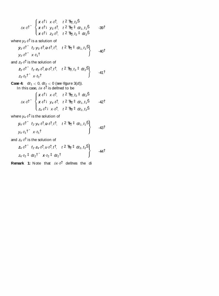
¯x…t† ˆxx…t† ¡ x…t†; t 2 ‰t1; t2Šxx…t† ¡ y3

…t†; t 2 ‰t1‡ dt1; t1

Šxx…t† ¡ z3

…t†; t 2 ‰t2; t2 ‡ dt2Š

8><>:

…39†

where y3…t† is a solution of

_yy3…t† ˆ f2…y3

…t†; uu…t†; t†; t 2 ‰t1‡ dt1; t1

Š

y3…t† ˆ x…t1

†

)…40†

and z3…t† is the solution of

_zz3…t† ˆ f2…z3

…t†; uu…t†; t†; t 2 ‰t2; t2‡ dt2

Š

z3…t2

† ˆ x…t2†

)

…41†

Case 4: dt1 < 0, dt2 < 0 (see ®gure 3(d)).In this case, ¯x…t† is de®ned to be

¯x…t† ˆxx…t† ¡ x…t†; t 2 ‰t1; t2 ‡ dt2

Š

xx…t† ¡ y4…t†; t 2 ‰t1

‡ dt1; t1Š

z4…t† ¡ x…t†; t 2 ‰t2

‡ dt2; t2Š

8>><>>:

…42†

where y4…t† is the solution of

_yy4…t† ˆ f2

…y4…t†; uu…t†; t†; t 2 ‰t1

‡ dt1; t1Š

y4…t1

† ˆ x…t1†

9=

; …43†

and z4…t† is the solution of

_zz4…t† ˆ f2

…z4…t†; u…t†; t†; t 2 ‰t2

‡ dt2; t2Š

z4…t2

‡ dt2† ˆ xx…t2

‡ dt2†

9=

; …44†

Remark 1: Note that ¯x…t† de®nes the di� erencebetween xx…t† and x…t† in the time interval where subsys-tem 2 is active. Moreover, by extending the trajectories xxand x under subsystem 2 dynamics to the time intervalmin ft1; t1

‡ dt1g µ t µ max ft2; t2 ‡ dt2g where at least

one of xx…t† and x…t† evolves along subsystem 2, ¯x…t†even de®nes the di� erence for this time interval.

In the following, the expressions for ¯x…t2† and

dx…t2† are derived. The following important Lemma 2

will be used frequently in the proofs of the lemmas inthis section (for details see Appendix A).

Lemma 2 (Pontryagin et al. 1964): Let g…t; u† be areal continuous function of the pair of variablest 2 …a; b†, u 2 Y ³ m and let u…t†, a < t < b, be apiecewise continuous function with values in U. If ³ is apoint in …a; b† and one of the following three conditionsis satis®ed

(a) ³ is a point at which u is continuous and p; q arearbitrary real numbers.

(b) ³ is a point at which u is right continuous and bothp; q are positive.

(c) ³ is a point at which u is left continuous and bothp; q are negative,

then we have

…³‡q°

³‡p°g…t; u…t†† dt ˆ °…q ¡ p†g…³; u…³†† ‡ o…°† …45†

Here ° is a su� ciently small positive number, and o…°† is anin®nitesimal of higher order than °, i.e. lim°! 0 o…°†=° ˆ 0.

Remark 2: In Pontryagin et al. (1964), Lemma 2 issaid to hold for almost every ³ in the case of measur-able function u. Here for our purpose in this paper, werestrict u to be piecewise continuous functions.

Lemma 3: The expressions of ¯x…t2† and ¯x…t2 ‡ dt2†are

¯x…t2† ˆ A…t2; t1†… f

1¡ ¡ f1‡† dt1

‡ o…dt1† …46†

¯x…t2 ‡ dt2† ˆ A…t2; t1†… f

¡1 ¡ f 1‡† dt1

‡ f 2¡x A…t2; t1†… f

¡1 ¡ f 1‡† dt1 dt2

‡ …other terms in dt21; dt

22

and higher order terms† …47†

where A…t2; t1† is the state transition matrix for the vari-

ational time-varying equation

_yy…t† ˆ @f …x…t†; u…t†; t†@x

y…t† …48†

for y…t†, t 2 ‰t1; t2Š; in …48†, f is the corresponding active

subsystem vector ®eld (here it is f2) in ‰t1; t2Š and u; x are

the current nominal input and state.

Proof: See Appendix A. &

In fact, from the proof of Lemma 2 (see AppendixA), we can observe that ¯x…t† ˆ A…t; t1

†¯x…t1† ‡ o…dt1

†for any t 2 ‰min ft1; t1

‡ dt1g, max ft2; t2

‡ dt2gŠ. The

following important principle can be obtained directlyfrom this observation. We refer to it as the forwarddecoupling principle in the subsequent discussions. Itreveals some intrinsic relationship among di� erentswitching instants.

The forward decoupling principle: If u assumes open-loop variations, then:

(a) The value of the incremental change ¯x…t1† at t1

will not be dependent upon dt2.

(b) The value of the incremental change ¯x…t2† at t2

will be dependent upon dt2.

The forward decoupling principle tells us that avariation of an earlier switching instant will a� ect thevalue of the incremental change at a later switchinginstant, but not vice versa.

Lemma 4: The expression of dx…t2† is

1414 X. Xu and P. J. Antsaklis

Dow

nloa

ded

by [

Otto

-von

-Gue

rick

e-U

nive

rsita

et M

agde

burg

] at

03:

08 2

2 O

ctob

er 2

014

dx…t2† ˆ A…t1; t1

†… f¡1 ¡ f

1‡† dt1

‡ f2¡x A…t2; t1

†… f1¡ ¡ f

1‡† dt1dt2‡ f

2¡dt2

‡ …other terms in dt21; dt2

2

and higher order terms† …49†

Proof: The proof follows directly from the fact that

dx…t2† ˆ ¯x…t2

‡ dt2† ‡ f2

…x…t2†; u…t2

¡†; t2† dt2‡ o…dt2

†…50†

for all four cases of the signs of dt1; dt2. &

Remark 3: It is very important to point out that inthe expression of dx…t2†, we deliberately express theterm f 2¡

x A…t2; t1†… f 1¡ ¡ f 1‡† dt1 dt2 explicitly because itwill contribute to the coe� cient of dt1 dt2 as can beseen from the discussions below.

Now that we have the expressions for ¯x…t2†,

¯x…t2‡ dt2

† and dx…t2†, we are ready to derive the coef-

®cient for dt1 dt2 in the expansion of

V0…x0; t0; t1

‡ dt1; t2‡ dt2

† ˆ V2…xx…t2

‡ dt2†; t2

‡ dt2†

‡…

t2‡dt2

t0

L…xx…t†; uu…t†; t† dt

…51†

There are two terms in (51). Let us look at theirTaylor expansions one by one in order to ®nd eachterm’s contribution to the coe� cient of dt1 dt2.

Similar to the single switching case, the Taylorexpansion of the ®rst term is

V2…xx…t2

‡ dt2†; t2 ‡ dt2† ˆ V

2‡ ‡ V2‡x dx…t2

† ‡ V2‡t2

dt2

‡ 12…dx…t2

††TV

2‡xx dx…t2

†

‡ 12V

2‡t2 t2 dt

22

‡ dt2V2‡t2x dx…t2†

‡ o…dt22† …52†

In (52), the terms that will possibly contribute to thecoe� cient of dt1 dt2 are those containing dx…t2

†. Theyare

V2‡x dx…t2

†; 12…dx…t2

††TV

2‡xx dx…t2

†; dt2V2‡t2x dx…t2

†…53†

Substituting the expression of dx…t2† into (53) and sum-

ming them, we obtain the contribution of the ®rst termto the coe� cient of dt1 dt2 as

‰V2‡x f 2¡

x‡ … f 2¡†T

V2‡xx

‡ V2‡t2x

ŠA…t2; t1†… f 1¡ ¡ f 1‡† …54†

For the second term in (51), we have the followinglemma.

Lemma 5: The contribution of„

t2‡dt2

t0L…xx; uu; t† dt to the

coe� cient of dt1 dt2 is

L2¡x A…t2; t1

†… f1¡ ¡ f

1‡† …55†

Proof: See Appendix A. &

Remark 4: The above results still hold even whent1 ˆ t2 (we can consider t2 > t1 ®rst and then lett2 ! t1 to prove this).

Combining (54) and (55) and the expression of V2‡t2x

which can be obtained similarly to the expression of V1‡t1x

in (27), we conclude that the coe� cient of dt1 dt2 (i.e.V

0t1 t2

in the expansion of V0…x0; t0; t1

‡ dt1; t2 ‡ dt3† is

V0t1 t2

ˆ ‰V2‡x f

2¡x

‡ … f2¡†T

V2‡xx

‡ V2‡t2x

‡ L2¡x

Š

£ A…t2; t1†… f

1¡ ¡ f1‡†

ˆ ‰V2‡x

… f 2¡x

¡ f 2‡x

† ‡ … f 2¡ ¡ f 2‡†TV2‡

xx‡ L2

x¡ L2‡

xŠ

£ A…t2; t1†… f

1¡ ¡ f1‡† …56†

The above result can also be similarly extended tothe case of K switchings to relate ¯x…tl

† and dtk (k < l).The expression for V

0tktl

can similarly be obtained. Wesummarize and extend the results obtained in this sec-tion into the following theorem.

Theorem 1: For a switched system with K switchings

V0…x0; t0; t1

‡ dt1; t2‡ dt2; . . . ; tK

‡ dtK†

ˆ V0…x0; t0; t1; t2; . . . ; tK

† ‡XK

kˆ1

V0tk dtk

‡12

XK

kˆ1

V0tktk

dt2k

‡X

1µk<lµK

V0tktl dtk dtl

‡ …higher order terms† …57†

where

V0tk

ˆ Lk¡ ¡ L

k‡ ‡ Vk‡x

… fk¡ ¡ f

k‡† …58†

V0tk tk

ˆ … f k¡ ¡ f k‡†TVk‡

xx… f k¡ ¡ f k‡†

¡ …Vk‡x f k‡

x‡ Lk‡

x†… f k¡ ¡ f k‡†

‡ …Vk‡x

… fk¡x

¡ fk‡x

† ‡ Lk¡x

¡ Lk‡x

†f k¡

‡ Vk‡x

… fk¡t

¡ fk‡t

† ‡ Lk¡t

¡ Lk‡t

‡ …Vk‡x f k¡

u‡ Lk¡

u† _uu

k¡ ¡ …Vk‡x f k‡

u‡ Lk‡

u† _uu

k‡ …59†

V0tktl

ˆ ‰V l‡x

… fl¡x

¡ fl‡x

† ‡ … fl¡ ¡ f

l‡†TV

l‡xx

‡ Ll¡x

¡ Ll‡x

ŠA…tl; tk†… f k¡ ¡ f k‡† …60†

Optimal control of switched systems 1415

Dow

nloa

ded

by [

Otto

-von

-Gue

rick

e-U

nive

rsita

et M

agde

burg

] at

03:

08 2

2 O

ctob

er 2

014

5.3. The implementation of the algorithm

Once the values of @V0=@ tt and @

2V

0=@ tt

2are obtained

as approximations to @J1=@ tt and @2J1=@ tt

2, the following

algorithm which is a modi®ed version of the conceptualAlgorithm 2 can be used for Stage 1 optimization.

Algorithm 3ÐAlgorithm for Stage 1 optimization:

Step 1. Set the iteration index j ˆ 0. Choose an initialtt

j.

Step 2. By solving an optimal control problem for thecurrent tt

j(Stage 1(a)), ®nd the corresponding

optimal or suboptimal control input uj.

Step 3. For the current ttj

and its corresponding uj,

supping that uj

assumed open-loop variations,®nd …@V 0

=@ tt†…tt j† and …@2V0=@ tt2†…tt j† as ap-

proximations to @J1=@ tt and @2J1=@ tt2.

Step 4. Use some feasible direction method to updatett j µ 0 to be tt j‡1 ˆ tt j ‡ ¬

j dtt j. Set the iterationindex j ˆ j ‡ 1.

Step 5. Repeat Steps 2, 3, 4 and 5, until a prespeci-®ed termination condition is satis®ed (e.g.k…@V

0=@ tt†…tt j†k < ° where ° is a given small

number).

It should be pointed out that in order to compute…@V

0=@ tt†…tt j† and …@2

V0=@ tt

2†…tt j† using the formulae(58)±(60), we need to know the values of V

k‡x , V

k‡xx ,

_uuk¡

, _uuk‡

and A…tl; tk†. However, given nominal tt, u

and x, these values are not readily available. In general,numerical methods need to be used to approximate theirvalues. Appendix B presents a possible way to approx-imate their values and solve Stage 1 optimization prob-lems although it is not the only method. Note that suchnumerical methods often demand extra computationale� ort. However, for the special class of optimal controlproblems which are called generalized switched linearquadratic (GSLQ) problems, the methods in }} 5.1 and5.2 can be modi®ed so that these values can be easilyobtained. We will elaborate on this in the next section.

Another thing we need to note is the di� erentiabilityof J1 and V 0. In general, for conventional optimal con-trol problems, the optimal value function is not di� er-entiable as a function of the initial point, especially whenthe problem has state or control constraints. However,here V0 is the cost value given the nominal u…t† and ttand it is not necessarily optimal. It can observed thatwhen the switching instants are slightly disturbed, thiscost value will also vary slightly; therefore it is contin-uous and even di� erentiable. As from our computa-tional experience, when the subsystems are smoothenough, the function J1

…tt† is also di� erentiable; in par-ticular this can be justi®ed for GSLQ problems usingarguments from ordinary di� erential equation theory.Due to this reason, in this paper we assume the di� er-

entiability of the value function and its approximationsunder the assumption that the subsystem dynamics aresmooth enough.

6. General switched linear quadratic problems

In this section, we adopt the approach in } 5 and useit for a general switched linear quadratic (GSLQ) prob-lem (Problem 6.1). Using the modi®ed approach for thisclass of problems, the implementation issues mentionedat the end of Section 5.3 can be successfully addressed.

Problem 2ÐGSLQ problem: Consider a switched sys-tem S ˆ …D; F † with linear subsystems _xx ˆ Aix ‡ Biu,i 2 I . Given a ®xed time interval ‰t0; tf Š, ®nd a con-tinuous input u 2 U ‰t0;tf Š and a switching sequence

¼ 2 S‰t0;tf Š such that the cost functional in generalquadratic form

J ˆ 12x

…tf†T

Qf x…tf† ‡ Mf x…tf

† ‡ Wf

‡…

tf

t0

…12x

TQx ‡ xTVu ‡ 12u

TRu ‡ Mx ‡ Nu ‡ W† dt

…61†

is minimized. Here t0, tf and x…t0† ˆ x0 are given; Qf ,

Mf , Wf , Q, V , R, M, N, W are matrices of appropriatedimensions with Qf

¶ 0, Q ¶ 0 and R > 0.

In comparison to the cost functionals of standardLQR control problems, here the cost functional J hasthe terms Mf

…xf†, Wf , x

TVu, Mx, Nu and W . In this

way, we can address more general problems such astracking of a constant trajectory, controlling the ®nalstate to a target, etc.

6.1. Solution for a single linear system

Note that for the general quadratic control of asingle linear system _xx ˆ Ax ‡ Bu, we can use thedynamic programming approach to obtain the followingresults (see Basar and Olsder (1999) for more on dynamicprogramming).

The optimal value function is

V¤…x; t† ˆ 1

2xTP…t†x ‡ S…t†x ‡ T…t† …62†

where P…t† ˆ PT…t† and

¡ _PP…t† ˆ Q ‡ P…t†A ‡ ATP…t†

¡ …P…t†B ‡ V†R¡1…BTP…t† ‡ V

T† …63†

¡ _SS…t† ˆ M ‡ S…t†A ¡ …N ‡ S…t†B†

£ R¡1…BT

P…t† ‡ VT† …64†

¡ _TT…t† ˆ W ¡ 12…N ‡ S…t†B†R¡1…BTST…t† ‡ NT† …65†

1416 X. Xu and P. J. Antsaklis

Dow

nloa

ded

by [

Otto

-von

-Gue

rick

e-U

nive

rsita

et M

agde

burg

] at

03:

08 2

2 O

ctob

er 2

014

Note that the ®nal conditions for P, S and T are

P…tf† ˆ Qf , S…tf † ˆ Mf and T…tf

† ˆ Wf .The optimal control is in the feedback form

u…x…t†; t† ˆ ¡K…t†x…t† ¡ E…t† …66†

where

K…t† ˆ R¡1…BT

P…t† ‡ VT† …67†

E…t† ˆ R¡1…BTST…t† ‡ NT† …68†

Remark 5: For a GSLQ Stage 1(a) problem, if we as-

sume that subsystem (Ak; Bk) is active in t 2 ‰tk¡1; tk†,the above results also hold except that (63)±(68) shouldbe modi®ed by substituting A and B with Ak and Bk

in the time interval ‰tk¡1; tk† (AK‡1 and BK‡1 in ‰tK ; tf Š).

6.2. Modi®ed method for GSLQ problems

Now we adopt the method developed in } 5 for Stage

1 optimization in a GSLQ problem. Here Vk‡x , V

k‡xx , _uu

k¡

and _uuk¡

can be obtained more easily without much extracomputational e� ort. Assume we are given nominal

switching instants and the corresponding nominal opti-mal continuous input u…¢† is in feedback form (66). If wesubstitute the expression of u…¢† into the system equa-

tions, it would look as if K…¢†; E…¢† play the role of con-tinuous inputs. Therefore it is natural to assume that thefeedback coe� cients K…¢†; E…¢† rather than u…¢† have

open-loop variations. We now use on K and E anapproach analogous to the derivation of } 5. This can

give us the ¯exibility of letting u vary as a function of xsince here u depends on x (see (66)). We say that uassumes closed-loop variations in this case. Conse-

quently we have (compare with (27) and (28))

Vk‡tkx

ˆ ¡… fk‡1†T

Vk‡xx

¡ Vk‡x f

k‡x

¡ Lk‡x

¡ …Vk‡x f k‡

u‡ Lk‡

u†uk‡

x…69†

Vk‡tktk

ˆ ¡Vk‡tkxf

k‡ ¡ Vk‡x f

k‡t

¡ Lk‡t

¡ …Vk‡x f

k‡u

‡ Lk‡u

†uk‡t

ˆ … f k‡†TVk‡

xx f k‡ ‡ …Vk‡x f k‡

x‡ Lk‡

x†f k‡ ¡ Vk‡

x f k‡t

¡ Lk‡t

‡ …Vk‡x f k‡

u‡ Lk‡

u†…uk‡

u f k‡ ¡ uk‡t

† …70†

Note that the expressions Vk‡tkx and Vk‡

tktkare di� erent

from those in } 5.1. We can follow the similar procedureas in } 5.1 (by assuming that K and E have open-loop vari-ations) to show that V0

tkis of the same form as in Theorem 1

V0tk

ˆ Lk¡ ¡ L

k‡ ‡ Vk‡x

… fk¡ ¡ f

k‡† …71†

and by substituting (69), (70) into (25) it can be seen that

V0tk tk

ˆ … fk¡ ¡ f

k‡†TV

k‡xx

… fk¡ ¡ f

k‡†

¡ …Vk‡x f

k‡x

‡ Lk‡x

†… fk¡ ¡ f

k‡†

‡ …Vk‡x

… f k¡x

¡ f k‡x

† ‡ Lk¡x

¡ Lk‡x

†f k¡

‡ Vk‡x

… f k¡t

¡ f k‡t

† ‡ Lk¡t

¡ Lk‡t

‡ …Vk‡x f

k¡u

‡ Lk¡u

† _uuk¡ ¡ …Vk‡

x fk‡u

‡ Lk‡u

† _uuk‡

¡ 2…Vk‡x f

k‡u

‡ Lk‡u

†uk‡x

… fk¡ ¡ f

k‡† …72†

where

_uuk¡ ˆ u

k¡x f

k¡ ‡ uk¡t

…73†

_uuk‡ ˆ uk‡

x f k‡ ‡ uk‡t

…74†

V0tktl

can also be derived similarly to the derivation in} 5.2 except for the di� erence described below. Here wecan substitute u…x…t†; t† ˆ ¡K…t†x…t† ¡ E…t† into thesystem state equation and the cost functional. Notethat K and E assume open-loop variations and u is afunction of x; hence a variation ¯x will cause a variation

¯u ˆ ¡K…y†¯x. Similarly to the derivations in } 5.2, wecan prove that the expression of ¯x…tl

‡ dtl† is (comparewith (47))

¯x…tl‡ dtl

† ˆ A…tl ; tk†… f k¡ ¡ f k‡† dtk

‡ … f l¡x

‡ f l¡u ul¡

x†A…tl; tk

†… f k¡ ¡ f k‡† dtk dtl

‡ …other terms in dt2k; dt

2l

and higher order terms† …75†

where A…tl; tk† is the state transition matrix for

¯ _xx ˆ @f …x; u; t†@x

¯x ‡ @f …x; u; t†@u

¯u

ˆ …Ai…t† ¡ Bi…t†K…t††¯x …76†

Once we have the expression of ¯x…tl‡ dtl

†, we can simi-larly obtain (compare with (49))

dx…tl† ˆ A…tl; tk

†… fk¡ ¡ f

k‡† dtk‡ … f

l¡x

‡ fl¡u u

l¡x

†

£ A…tl; tk†… f

k¡ ¡ fk‡† dtk dtl

‡ fl¡

dtl

‡ …other terms in dt2k; dt

2l and higher order terms†

…77†

Moreover, similarly to the derivation in } 5.2, we canderive the coe� cient for dtk dtl in the expansion of V0…x0;t0; t1 ‡ dt1; . . . ; tk

‡ dtk; . . . ; tl‡ dtl; . . . ; tK ‡ dtK

† as

V0tk tl

ˆ ‰V l‡x

… fl‡x

¡ fl¡x

† ‡ … fl¡ ¡ f

l‡†TV

l‡xx

‡ …Ll¡x

¡ Ll‡x

†

‡ …Ll¡u u

l¡x

¡ Ll‡u u

l‡x

†ŠA…tl; tk†… f

k¡ ¡ fk‡† …78†

It can now be seen from the expressions of V0tk , V

0tk tk and

V0tk tl that all terms necessary for the evaluation of them

are readily available. In particular, in this case

Optimal control of switched systems 1417

Dow

nloa

ded

by [

Otto

-von

-Gue

rick

e-U

nive

rsita

et M

agde

burg

] at

03:

08 2

2 O

ctob

er 2

014

Vk‡x

ˆ xT…tk†Pk‡ ‡ Sk‡ …79†

Vk‡xx

ˆ Pk‡ …80†

_uuk¡ ˆ ¡ _KK

k¡x…tk

† ¡ Kk¡

fk¡ ¡ _EE

k¡ …81†

_uuk‡ ˆ ¡ _KK

k‡x…tk

† ¡ Kk‡

fk‡ ¡ _EE

k‡ …82†

uk¡x

ˆ ¡Kk¡ …83†

uk‡x

ˆ ¡Kk‡ …84†

ul¡x

ˆ ¡K l¡ …85†

ul‡x

ˆ ¡Kl‡ …86†

where x, P and S are continuous at tk; _KKk¡, _KKk‡

, _EEk¡

and _EEk‡are functions of P and S obtainable by substi-

tuting the expressions of _PP and _SS into the di� erentia-tions of (67) and (68). Note that the values of P, S and Tcan be obtained by solving the Riccati equations (63)±(65) along with the ®nal conditions P…tf

† ˆ Qf , S…tf† ˆ

Mf and T…tf† ˆ Wf (except that it will now go through

K ‡ 1 subsystems instead of only 1 subsystem). Theadvantage of applying the approach to GSLQ problemsis that here V

k‡x , V

k¡xx , _uu

k¡and _uu

k‡can be obtained easily

without resorting to extra computational methods.A…tl; tk

† is the state transition matrix from tk to tl forthe time varying linear system

_yy…t† ˆ …Ai…t† ¡ Bi…t†K…t††y…t† …87†

which can be calculated by numerical integrations asfollows.

For the current nominal x…t†, u…t†, K…t† and nominalswitching instants, ®nd the solutions y1

…t†; . . . ; yn…t† for

(87) that corresponds to the initial conditions

y1…tk

† ˆ e1; . . . ; yn…tk

† ˆ en…88†

where ej is the unit column vector that has all 0s exceptfor a 1 as the jth element, j ˆ 1; 2; . . . ; n. From linearsystems theory, we observe that A…tl; tk

† can be approxi-mated by the square matrix whose jth coumn is yj

…tl†,

i.e.

A…tl; tk† ˆ ‰y1

…tl†; . . . ; yn…tl

†Š …89†

Now that we have the expressions for V0tk

, V0tktk and

V0tktl

, we can use Algorithm 3 except that Step 3 shouldbe revised as `suppose K and E assumes open-loop vari-ations’.

Remark 6: It should be pointed out that only closed-loop variations for u can give us the convenience ofcomputing Vk‡

x , Vk‡xx , _uuk¡

and _uuk‡. If open-loop varia-

tions for u is adopted, the relationship V…x; t† ˆ12 xTP…t†x ‡ S…t†x ‡ T…t† is no longer true; hence (79)±(86) cannot be used. In such a case, computationalmethods such as the method mentioned in Appendix Bneed to be derived to ®nd approximations for the re-quired values.

7. Some examples

In this section, we illustrate the e� ectiveness of theapproach developed in the last two sections using threeexamples. The ®rst has non-linear subsystems and thelast two have linear subsystems. For more examples ofthe application of the method to general non-linearswitched systems, please refer to Xu (2001).

Example 2: Consider a switched system consisting of

subsystem 1:_xx1

ˆ ¡x1‡ 2x1u

_xx2ˆ x2

‡ x2u

8<

: …90†

subsystem 2:_xx1

ˆ x1¡ 3x1u

_xx2ˆ 2x2

¡ 2x2u

8<

: …91†

subsystem 3:_xx1

ˆ 2x1‡ x1u

_xx2ˆ ¡x2

‡ 3x2u

8<

: …92†

Assume that t0ˆ 0, tf

ˆ 3 and the system switches att ˆ t1 from subsystem 1 to 2 and at t ˆ t2 from subsys-tem 2 to 3 (0 µ t1

µ t2µ 3). We want to ®nd optimal

switching instants t1; t2 and an optimal input u such thatthe cost functional

J ˆ 12…x1

…3† ¡ 2†2 ‡ 12…x2

…3† ¡ 2†2

‡ 12

…3

0

…x1…t† ¡ 2†2 ‡ …x2

…t† ¡ 2†2 ‡ u2…t† dt

is minimized. Here x1…0† ˆ 1 and x2

…0† ˆ 1.For this problem, we choose initial nominal t1 ˆ 1,

t2ˆ 2. By using Algorithm 3 with the constrained

Newton’s method (implemented using the method inAppendix B), after 19 iterations we ®nd that the optimalswitching instants are t1

ˆ 0:0001, t2ˆ 1:7244 and the

corresponding optimal cost is 3.6250. From this result,we ®nd that in the optimal solution, subsystem 1 shouldnot be active (the reason we still have t1

ˆ 0:0001 here isdue to numerical tolerance). The system only needs toswitch from subsystem 2 to 3 at t2

ˆ 1:7244. The corre-sponding continuous control and state trajectory areshown in ®gure 4(a) and (b).

Example 3: Consider a switched system consisting of

subsystem 1: _xx ˆ0:6 1:2

¡0:8 3:4

2

4

3

5x ‡1

1

2

4

3

5u …93†

subsystem 2: _xx ˆ4 3

¡1 0

2

4

3

5x ‡2

¡1

2

4

3

5u …94†

1418 X. Xu and P. J. Antsaklis

Dow

nloa

ded

by [

Otto

-von

-Gue

rick

e-U

nive

rsita

et M

agde

burg

] at

03:

08 2

2 O

ctob

er 2

014

Assume that t0ˆ 0, tf

ˆ 2 and the system switches onceat t ˆ t1 (0 µ t1

µ 2) from subsystem 1 to 2. We want to®nd an optimal switching instant t1 and an optimalinput u such that the cost functional

J ˆ 12…x1

…2† ¡ 4†2 ‡ 12…x2

…2† ¡ 2†2

‡ 12

…2

0

…x2…t† ¡ 2†2 ‡ u2…t† dt …95†

is minimized. Here x…0† ˆ ‰0; 2ŠT.

For this GSLQ problem, we use the modi®ed

method for GSLQ problems to obtain approximations

to dJ1=dt1. From an initial nominal t1ˆ 1:0, by using

Algorithm 3 with the gradient projection method, after13 iterations we ®nd that the optimal switching instant is

t1ˆ 0:1897 and the corresponding optimal cost is

9.7667. The corresponding continuous control and

state trajectory are shown in ®gure 5(a) and (b).

Figure 6 shows the optimal cost for di� erent t1s.

Example 4: Consider a switched system consisting of

subsystem 1: _xx ˆ¡2 0

0 ¡1

" #

x ‡1

0

" #…96†

subsystem 2: _xx ˆ0:5 5:3

¡5:3 0:5

" #

x ‡1

¡1

" #…97†

subsystem 3: _xx ˆ1 0

0 1:5

" #

x ‡0

1

" #

u …98†

Assume that t0ˆ 0, tf

ˆ 3 and the system switches at

t ˆ t1 from subsystem 1 to 2 and at t ˆ t2 from subsys-tem 2 to 3 (0 µ t1

µ t2µ 3). We want to ®nd optimal

Optimal control of switched systems 1419

Figure 4. Example 2: (a) The control input. (b) The state trajectory.

Figure 5. Example 3: (a) The control input. (b) The state trajectory.

Figure 6. The optimal cost for Example 3 for di� erent t1s.

Dow

nloa

ded

by [

Otto

-von

-Gue

rick

e-U

nive

rsita

et M

agde

burg

] at

03:

08 2

2 O

ctob

er 2

014

switching instants t1; t2 and an optimal input u such thatthe cost functional

J ˆ ‰…x1…3† ‡ 4:1437†2 ‡ …x2

…3† ¡ 9:3569†2Š ‡ 12

…3

0u

2…t† dt

…99†

is minimized. Here x…0† ˆ ‰4; 4ŠT.For the GSLQ problem, we use the modi®ed method

for GSLQ problems to obtain approximations to @J1=@ ttand @

2J1=@ tt2. From initial nominal values t1

ˆ 0:8,t2

ˆ 1:8, by using Algorithm 3 with the constrainedNewton’s method, after 43 iterations we ®nd that theoptimal switching instant is t1

ˆ 1:0002, t2ˆ 2:0008

and the corresponding optimal cost is 6:3146 £ 10¡5

.The corresponding continuous control and state trajec-tory are shown in ®gure 7(a) and (b). Note that thetheoretical optimal solutions for this problem aretopt1

ˆ 1, topt2

ˆ 2, uopt ² 0 and J

opt ˆ 0, so the resultwe obtained is quite accurate. Figure 8 shows the opti-mal cost for di� erent t1 < t2.

For this example, we have deliberately selected thedesired x1

…3† and x2…3† so that the theoretical optimal

solution will be topt1

ˆ 1, topt2

ˆ 2. In this way, we cancheck the validity of our result by comparing it withthe theoretical result. It can be observed from ®gure 8that the function J1

…t1; t2† has several ripples. Such non-

convexity is typical and it occurs even in this simpleGSLQ problem. This perhaps can explain why suchproblems pose signi®cant di� culties. Another thing tonote is that by using constrained non-linear optimiza-tion for Stage 1(b), the solution we found is a localminimum. In order to search for a global minimum,we might need to start with an initial guess close tothe global minimum as we did in this example, or wemight try di� erent initial guesses to obtain the best localminimum.

The optimal control solutions in the above three ex-amples were derived using the algorithms in }} 5 and 6and implemented in Matlab.

8. Conclusions

In this paper, we formulated a general optimal con-trol problem for switched systems and proposed a twostage optimization methodology for it. Then we focusedon Stage 1 optimization problem which was furtherdecomposed into Stage 1(a) and Stage 1(b). We pro-posed a method to obtain approximations of the deri-vative information that is necessary for Stage 1(b)optimization (Stage 1(a) is solved using standard opti-mal control methodologies). The method is based ondirect di� erentiations of value functions (Theorem 1).A modi®ed version of the method was then proposedfor general switched linear quadratic (GSLQ) problemswhich can successfully address some of the implementa-tion di� culties of the general method. Note that earlierresults of this paper have appeared in Xu and Antsaklis2000 a, b, 2001) and a more complete version can befound in Xu (2001). There are many further researchtopics that are worth exploring. One is detailed conver-

1420 X. Xu and P. J. Antsaklis

Figure 7. Example 4: (a) The control input. (b) The state trajectory.

Figure 8. The optimal cost for Example 4 for di� erent …t1; t2†s(0 µ t1 µ t

2 µ 3).

Dow

nloa

ded

by [

Otto

-von

-Gue

rick

e-U

nive

rsita

et M

agde

burg

] at

03:

08 2

2 O

ctob

er 2

014

gence analysis and exploration of methods to accelerateconvergence, for example modifying the search direc-tions similarly to the conjugate direction methods infunction optimization. Other topics include the develop-ment of numerical methods for deriving accurate valuesof @J1=@ tt, @

2J1=@ tt2; development of methods for Stage 1optimization for systems with state and control con-straints; explorations of the properties of the functionJ1

…tt†, etc. We will report progress in these topics infuture papers.

Acknowledgements

The research in this paper is supported by the ArmyResearch O� ce (DAAG 55-98-1-0199 ) and NationalScience Foundation (NSF ECS-9912458).

Appendix A: Some proofs for § 5.2

Proof of Lemma 3: Although the results in the lemmahold for all cases in the de®nition of ¯x…t†, we need todiscuss each case in order to show the validity of them.

Case 1: dt1 ¶ 0, dt2 ¶ 0.

¯x…t1‡ dt1

† ˆ…

t1‡dt1

t1

f1…xx…t†; uu…t†; t† dt

¡…

t1‡dt1

t1

f2…x…t†; u…t†; t† dt …100†

Using Lemma 2 (here we can let ° ˆ dt1, q ˆ 1 andp ˆ 0) and noting that xx…t1

† ˆ x…t1†, uu…t1

† ˆ u…t1¡†, we

have…

t1‡dt1

t1

f1…xx…t†; uu…t†; t† dt ˆ f1

…xx…t1†; uu…t1

†; t1† dt1

‡ o…dt1†

ˆ f1…x…t1

†; u…t1¡†; t1

† dt1‡ o…dt1

†

ˆ f 1¡dt1

‡ o…dt1† …101†

Using Lemma 2, we have…

t1‡dt1

t1

f2…x…t†; u…t†; t† dt ˆ f2

…x…t1†; u…t1

‡†; t1† dt1

‡ o…dt1†

ˆ f1‡

dt1‡ o…dt1

† …102†

Hence ¯x…t1 ‡ dt1† ˆ … f

¡1 ¡ f1‡† dt1

‡ o…dt1† and we

conclude from the property of the variational equationthat

¯x…t2† ˆ A…t2; t1 ‡ dt1

†¯x…t1‡ dt1

† ‡ o…dt1†

ˆ ‰A…t2; t1† ‡ At1 dt1

‡ o…dt1†Š

£ ‰…f 1¡ ¡ f1‡† dt1

‡ o…dt1†Š ‡ o…dt1

†

ˆ A…t2; t1†… f 1¡ ¡ f 1‡† dt1‡ o…dt1

† …103†

¯x…t2 ‡ dt2† ˆ xx…t2† ‡…

t2‡dt2

t2

f2…xx…t†; uu…t†; t† dt

µ ¶

¡ z1…t2† ‡…

t2‡dt2

t2

f2…z1…t†; uu…t†; t† dt†µ ¶

ˆ ¯x…t2† ‡…

t2‡dt2

t2

‰ f 2…xx…t†; uu…t†; t†

¡ f2…z1…t†; uu…t†; t†Š dt

ˆ ¯x…t2† ‡ ‰ f2…xx…t2†; u…t2¡†; t2†

¡ f2…x…t2†; u…t2¡†; t2†Š dt2 ‡ o…dt2†

ˆ ¯x…t2† ‡ f 2¡x ¯x…t2†; dt2 ‡ o…dt2†

ˆ A…t2; t1†… f 1¡ ¡ f 1‡† dt1dt2

‡ f 2¡x A…t2; t1†… f

¡1 ¡ f 1‡† dt1 dt2

‡ …other terms in dt21; dt2

2

and higher order terms†: …104†

Case 2: dt1 ¶ 0, dt2 < 0.The arguments for proving (103) in Case 1 can be

aplied in this case to show its validity. In this case,

¯x…t2‡ dt2

† ˆ z2…t2

‡ dt2† ¡ x…t2

‡ dt2†

ˆ z2…t2

† ‡…

t2‡dt2

t2

f2…z2

…t†; u…t†; t† dt

µ ¶

¡ x…t2† ‡

…t2

‡dt2

t2

f2…x…t†; u…t†; t† dt

µ ¶

ˆ ¯x…t2† ‡…

t2‡dt2

t2

‰ f2…z2

…t†; u…t†; t†

¡ f2…x…t†; u…t†; t†Š dt

ˆ ¯x…t2† ‡ ‰ f2…z2

…t2†; u…t2¡†; t2

†

¡ f2…x…t2†; u…t2¡†; t2†Š dt2

‡ o…dt2†

ˆ ¯x…t2† ‡ f2¡x ¯x…t2

† dt2‡ o…dt2

†

ˆ A…t2; t1†… f

1¡ ¡ f1‡† dt1

‡ f 2¡x A…t2; t1

†… f 1¡ ¡ f 1‡† dt1 dt2

‡ …other terms in dt21; dt2

2

and higher order terms) …105†

Case 3: dt1 < 0, dt2¶ 0.

In this case, we have

Optimal control of switched systems 1421

Dow

nloa

ded

by [

Otto

-von

-Gue

rick

e-U

nive

rsita

et M

agde

burg

] at

03:

08 2

2 O

ctob

er 2

014

¯x…t1† ˆ

…t1

t1‡dt1

f2…xx…t†; uu…t†; t† dt

¡…

t1

t1‡dt1

f1…x…t†; u…t†; t† dt

ˆ f2…x…t1

¡ dt1†; u…t1

‡†

‡ _uu1‡

dt1; t1 ‡ dt1†…¡dt1

†

¡ f1…x…t1 ‡ dt1

†; u…t1‡ dt1

†; t1‡ dt1

†

£ …¡dt1† ‡ o…dt1

†

ˆ f1…x…t1

†; u…t1¡†; t1

† dt1

¡ f2…x…t1†; u…t1

‡†; t1† dt1

‡ o…dt1†

ˆ … f 1¡ ¡ f 1‡† dt1‡ o…dt1

† …106†

In the derivations of the second to the last equationsin (106), we use the relationship

x…t1‡ dt1

† ˆ x…t1† ‡ _xx…t1

¡† dt1 ‡ o…dt1† …107†

u…t1‡ dt1

† ˆ u…t1¡† ‡ _uu…t1

¡† dt1‡ o…dt1

† …108†

and the Taylor expressions of f2 and f1. Therefore, wehave

¯x…t2† ˆ A…t2; t1

†¯x…t1† ‡ o…dt1

†

ˆ A…t2; t1†… f 1¡ ¡ f 1‡† dt1

‡ o…dt1† …109†

¯x…t2‡ dt2

† ˆ xx…t2† ‡

…t2

‡dt2

t2

f2…xx…t†; uu…t†; t† dt

µ ¶

¡ z3…t2

† ‡…

t2‡dt2

t2

f2…xx3

…t†; uu…t†; t† dt

µ ¶

ˆ ¯x…t2† ‡

…t2‡dt2

t2

‰ f2…~xx…t†; uu…t†; t†

¡ f2…z3…t†; uu…t†; t†Š dt

ˆ ¯x…t2† ‡ ‰ f2

…xx…t2†; u…t2

¡†; t2†

¡ f2…x…t2†; u…t2¡†; t2

†Š dt2‡ o…dt2

†

ˆ ¯x…t2† ‡ f 2¡

x ¯x…t2† dt2‡ o…dt2

†

ˆ A…t2; t1†… f

1¡ ¡ f1‡† dt1

‡ f2¡x A…t2; t1

†… f1¡ ¡ f

1‡† dt1 dt2

‡ …other terms in dt21; dt22 and

higher order terms† …110†

Case 4: dt1 < 0, dt2 < 0.

The arguments for proving (109) in Case 3 can beapplied in this case to show its validity. In this case,wehave

¯x…t2‡ dt2

† ˆ z4…t2

† ‡…

t2‡dt2

t2

f2…z4

…t†; u…t†; t† dt

µ ¶

¡ x…t2† ‡

…t2‡dt2

t2

f2…x…t†; u…t†; t† dt

µ ¶

ˆ ¯x…t2† ‡…

t2‡dt2

t2

‰ f2…z4

…t†; u…t†; t†

¡ f2…x…t†; u…t†; t†Š dt

ˆ ¯x…t2† ‡ ‰ f2…z4

…t2†; u…t2

¡†; t2†

¡ f2…x…t2†; u…t2¡†; t2

†Š dt2‡ o…dt2

†

ˆ ¯x…t2† ‡ f2¡x ¯x…t2

† dt2‡ o…dt2

†

ˆ A…t2; t1†… f

1¡ ¡ f1‡† dt1

‡ f2¡x A…t2; t1

†… f¡1 ¡ f

1‡† dt1 dt2

‡ …other terms in dt21; dt

22 and

higher order terms† …111†

Proof of Lemma 5: We ®rst note that…

t2‡dt2

t0

L…xx; uu; t† dt ˆ…

max ft1;t1‡dt1

g

t0

L…xx; uu; t† dt

‡…

t2‡dt2

max ft1;t1‡dt1g

L…x ‡ ¯x; uu; t†; dt

…112†

In the light of the forward decoupling principle, the ®rstterm in (112) will not depend on dt2; therefore, it will notcontribute to the coe� cient of dt1 dt2.

For the second term, we discuss as follows.

Case 1: dt2 ¶ 0.In this case, we have

…t2

‡dt2

max ft1;t1‡dt1

gL…xx; uu; t† dt ˆ

…t2

max ft1 ;t1‡dt1

gL…x ‡ ¯x; uu; t† dt

‡ L…~xx; uu; t† dt …113†

The ®rst term in (113) will not be contributing due to thereason that

¯x…t† ˆ A…t; t1†… f

1¡ ¡ f1‡† dt1

‡ o…dt1† …114†

uu…t† ˆ u…t† …115†

for t 2 ‰max ft1; t1‡ dt1

g; t2Š and therefore they are not

dependent upon dt2.

1422 X. Xu and P. J. Antsaklis

Dow

nloa

ded

by [

Otto

-von

-Gue

rick

e-U

nive

rsita

et M

agde

burg

] at

03:

08 2

2 O

ctob

er 2

014

The second term is shown to be…

t2‡dt2

t2

L…xx…t2†; uu…t†; t† dt ˆ L…xx…t2

†; u…t2¡†; t2

† dt2‡ o…dt2

†

ˆ L…x…t2†; u…t2

¡†; t2† dt2

‡ L2¡x ¯x…t2

† dt2

‡ …other terms in dt2; dt22 and

terms higher than order 2†

…116†

By substituting the expression of ¯x…t2† into (116),

we obtain the coe� cient of dt1 dt2 contributed by thisterm as

L2¡x A…t2; t1

†… f1¡ ¡ f

1‡† …117†

Case 2: dt2 < 0.In this case, since x…t† ‡ ¯x…t† ˆ xx…t† and uu…t† ˆ u…t†,

for t 2 ‰max ft1; t1 ‡ dt1g; t2

‡ dt2g, we have

…t2

‡dt2

max ft1;t1‡dt1

gL…xx; uu; t† dt ˆ

…t2

‡dt2

max ft1 ;t1‡dt1

gL…x ˆ ¯x; u; t† dt

ˆ…

t2

max ft1 ;t1‡dt1gL…x ‡ ¯x; u; t† dt

‡…

t2‡dt2

t2

L…x ‡ ¯x; u; t† dt

…118†

Similar to Case 1, the ®rst term in (118) will not becontributing. The second term is shown to be

…t2

‡dt2

t2

L…x ‡ ¯x; u; t† dt

ˆ L…x…t2† ‡ ¯x…t2

†; u…t2¡†; t2

† dt2‡ o…dt2

†

ˆ L…x…t2†; u…t2¡†; t2

† dt2‡ L

2¡x ¯x…t2

† dt2

‡…other terms in dt2; dt22

and terms higher than order 2† …119†

Therefore, by substituting the expression of ¯x…t2† into

(119), we obtain the same coe� cient (117). &

Appendix B: A numerical implementation of thealgorithm in § 5.3

A possible way to approximate the values of Vk‡x ,

Vk‡xx , _uu

k¡, _uu

k‡and A…tl; tk

† for the implementation ofAlgorithm 2 is described as follows. Suppose that thecurrent switching instant vector is tt ˆ …t1; . . . ; tK †T

andthe sequence of active subsystems is 1; 2; . . . ; K ; K ‡ 1.As mentioned in } 4, Stage 1(a) in which the switchinginstants are ®xed is actually a conventional optimal con-

trol problem. It can be solved by using a discrete-timeoptimal control agorithm for the discretized version ofthe continuous-time problem. Our computation of V

k‡x ,

Vk‡xx , _uu

k¡, _uu

k‡and A…tl; tk

† will be based on the solutionof the discretized optimal control problem.

In order not to lose the state, control information atthe switching instant, instead of discretizing the wholerange ‰t0; tf

Š using the same discretization level h (in thiscase, a switching instant may fail to be a grid point), wediscretize each interval ‰tk¡1; tk

Š into N intervals of equallength hk. In other words, for each ‰tk¡1; tk

Š we specify adi� erent discretization level hk (hKˆ1 for ‰tK ; tf

Š), hencethe total number of discretized intervals is …K ‡ 1†N . Inthis way, we can write our discretized system as

x…i ‡ 1† ˆ ff …x…i†; u…i†; i† …120†

ˆ

x…i† ‡ h1 f1…x…i†; u…i†; ih1

†;

0 µ i < N

x…i† ‡ h2 f2…x…i†; u…i†; Nh1 ‡ …i ¡ N†h2;

N µ i < 2N

..

.

x…i† ‡ hK‡1 fK‡1…x…i†; u…i†; N…h1 ‡ h2

‡ ¢ ¢ ¢ ‡ hK † ‡ …i ¡ KN†hK‡1†;

KN µ i < …K ‡ 1†N

…121†

8>>>>>>>>>>>>>>>>>><>>>>>>>>>>>>>>>>>>:

The corresponding discrete-time cost is

J ˆ ÁÁ…x……K ‡ 1†N†† ‡X…K‡1†N¡1

iˆ0

LL…x…i†; u…i†; i† …122†

where

ÁÁ…x……K ‡ 1†N†† ˆ Á…x……K ‡ 1†N†† …123†

LL…x…i†; u…i†; i† ˆ

h1L…x…i†; u…i†; ih1†;

0 µ i < N

h2L…x…i†; u…i†; Nh1‡ …i ¡ N†h2

†;

N µ i < 2N

..

.

hK‡1L…x…i†; u…i†; N…h1 ‡ h2

‡ ¢ ¢ ¢ ‡ hK† ‡ …i ¡ KN†hK‡1

†;

KN µ i < …K ‡ 1†N

…124†

8>>>>>>>>>>>>>>>>>>>>>>>><>>>>>>>>>>>>>>>>>>>>>>>>:

For the above discretized problem, Dyer andMcReynolds (1970) and Bertsekas (1999) not only pro-pose a ®rst-order method but also propose a second-order algorithm which is in feedback form. Here let usonly illustrate the ®rst-order algorithm for solving it

Optimal control of switched systems 1423

Dow

nloa

ded

by [

Otto

-von

-Gue

rick

e-U

nive

rsita

et M

agde

burg

] at

03:

08 2

2 O

ctob

er 2

014

(modi®ed using the Armijo stepsize rule (Bertsekas1999)). Here we de®ne the value function V not necess-arily optimal) corresponding to the control sequenceu…i†, i ˆ 0; 1; . . . ; …K ‡ 1†N ¡ 1 to be

V…x…i†; u…0†; u…1†; . . . ; u……K ‡ 1†N ¡ 1†; i†

7 ÁÁ…x……K ‡ 1†N†† ‡X…K‡1†N¡1

lˆi

L…x…l†; u…l†; l† …125†

It can be seen that V…i† actually only depend on x…i†,u…i†; u…i ‡ 1†; . . . ; u……K ‡ 1†N ¡ 1† and i. In the follow-ing, V…x…i†; u…0†; u…1†; . . . ; u……K ‡ 1†N ¡ 1†; i† is some-times denoted simply as V…i†.

Algorithm 4ÐFirst-order algorithm for the discretizedproblem:

Step 1. Set the iteration index j ˆ 0. Choose a nominalcontrol input u

j…i†, i ˆ 0; 1; . . . ; …K ‡ 1†N ¡ 1.Compute x

j…i†, i ˆ 0; 1; . . . ; …K ‡ 1†N from thesystem equation (120). Also compute the costV j…0†.

Step 2. Compute the partial derivatives

Vjx…i† 7 Vx

…x…i†; uj…0†; . . . ; u

j……K ‡ 1†N ¡ 1†; i†

Step 1. for i ˆ …K ‡ 1†N ; …K ‡ 1†N ¡ 1; . . . ; 0 from

Vjx……K ‡ 1†N ˆ ÁÁ

jx……K ‡ 1†N† …126†

Vjx…i† ˆ V

jx…i ‡ 1†ff j

x…i† ‡ LL

jx…i† …127†

Step 1. where

ÁÁjx……K ‡ 1†N† 7 ÁÁx

…x j……K ‡ 1†N††

ff jx

…i† 7 ffx…x j…i†; u j…i†; i†

LLjx…i† 7 LLx

…x j…i†; u j…i†; i†

Step 3. Compute and store the gradient with respect tothe control at each stage from

@Vj…0†

@u…i†ˆ @V

j…i†@u…i†

ˆ Vj

x…i ‡ 1†ff j

u…i† ˆ LL

ju…i†;

i ˆ …K ‡ 1†N ¡ 1; . . . ; 0 …128†

Step 1. where ff ju

…i† 7 ffu…x j…i†; u j…i†; i† and LL j

u…i† 7

LLu…x j…i†; u

j…i†; i†.Step 4. Use the Armijo stepsize rule to update the con-

trol (here we choose 0 < s, 0 < ­ < 1, 0 <¼ < 1

2). Let m¬ be the ®rst non-negative integerm for which

V j…x…0†; u j…0†; . . . ; u j……K ‡ 1†N ¡ 1†; 0†

¡V j

Á

x…0†; u j…0† ¡ ­m @V

j

@u…0†…0†; . . . ; u j

£……K ‡ 1†N ¡ 1† ¡ ­m

s@V

j

@u……K ‡ 1†N ¡ 1† …0†; 0

!

¶ ¼­ms

X…K‡1†N¡1

iˆ0

@Vj

@u…i†…0†

®®®®

®®®®2

2

…129†

Step 1. Set uj‡1…i† ˆ u

j…i† ¡ ­m¬ s…@V

j=@u…i††…0†, i ˆ 0;

1; . . . ; …K ‡ 1†N ¡ 1.

Step 5. Use the new control input u j‡1…i†, i ˆ0; 1; . . . ; …K ‡ 1†N ¡ 1 and the system equationsto construct new trajectory x

j‡1…i† and com-pute the new cost V j‡1…0†. Set the iterationindex j ˆ j ‡ 1.

Step 6. Repeat Steps 3, 4, 5 and 6 until a given numberof iterations have been completed, or the di� er-ence between the present V j…0† and the V j¡1…0†in last iteration is smaller than a given smalltolerance level ¯ > 0.

Remark 7: Note that Vx…i† is equal to the transposeof the costate varable p…i† (see Bertsekas 1999).

By using Algorithm 4, we can obtain the backwarddi� erence equations for Vx as

Vx……K ‡ 1†N† ˆ ÁÁx

……K ‡ 1†N† …130†

Vx…i† ˆ Vx

…i ‡ 1†ffx…i† ‡ LLx

…i† …131†

We can then approximate Vk‡x by

Vk‡x

� Vx…kN† …132†

Therefore, Vk‡x can be derived from solutions of (130)

and (131).Di� erentiating (130) and (131) with respect to x, we

obtain

Vxx……K ‡ 1†N† ˆ ÁÁxx

…x……K ‡ 1†N†† …133†

Vxx…i† ˆ ff T

x…i†Vxx

…i ‡ 1†ffx…i†

‡ Vx…i ‡ 1†ffxx

…i† ‡ LLxx…i† …134†

In (134), ffxx…i† is an n £ n £ n array whose ( j1; j2; j3)

element is @2 ffj1=@xj2 @xj3 and the notation

Vx…i ‡ 1†ffxx

…i† denotes an n £ n matrix which has its(j2; j3)th element as

Xn

j1ˆ1

Vxj1

…i ‡ 1† @2ffj1

@xj2 @xj3

…135†

1424 X. Xu and P. J. Antsaklis

Dow

nloa

ded

by [

Otto

-von

-Gue

rick

e-U

nive

rsita

et M

agde

burg

] at

03:

08 2

2 O

ctob

er 2

014

By solving (133) and (134) backwards in time, we canobtain Vxx

…i†. Then we can approximate Vk‡xx by

Vk‡xx

� Vxx…kN† …136†

Furthermore, we approximate _uuk¡

; _uuk‡

by

_uuk¡ ˆ u…kN ¡ 1† ¡ u…kN ¡ 2†

hk

…137†

_uuk‡ ˆ u…kN ‡ 2† ¡ u…kN ‡ 1†

hk‡1

…138†

Finally, we derive the approximation for A…tl; tk†.Note that A…tl; tk† is the state transition matrix for

_yy…t† ˆ @f …x; u; t†@t

y…t† …139†

For k < l, the discretized version of (139) for t 2 ‰tk; tlŠ is

y…i ‡ 1† ˆ

y…i† ‡ hk‡1@fk‡1

@x…x…i†; u…i†; N…h1

‡ ¢ ¢ ¢ ‡ hk†

‡…i ¡ kN†hk‡1†y…i†;

for kN µ i < …k ‡ 1†N

..

.

y…i† ‡ hl@fl

@x…x…i†; u…i†; N…h1

‡ ¢ ¢ ¢ ‡ hl¡1†

‡…i ¡ …l ¡ 1†N†hl†y…i†;

for …l ¡ 1†N µ i < lN

8>>>>>>>>>>>>>>>>>><>>>>>>>>>>>>>>>>>>:

…140†

Find the solution y…i†…i†; . . . ; y

…n†…i† corresponding toinitial conditions

y…1†…kN† ˆ e1; . . . ; y

…n†…kN† ˆ en…141†

respectively, where ej is the unit column vector with all0s except that the jth element is 1, j ˆ 1; 2; . . . ; n. Fromlinear systems theory, we oberve that A…tl; tk

† can beapproximated by the square matrix whose jth columnis y

…j†…lN†, i.e.

A…tl; tk† � ‰ y…1†…lN†; . . . ; y

…n†…lN†Š …142†

ReferencesAthans, M., and Falb, P., 1966, Optimal Control (New York:

McGraw-Hill).BasË ar, T., and Olsder, G. J., 1999, Dynamic Noncooperative

Game Theory, 2nd edn (Philadelphia, PA: SIAM).Bertsekas, D. P., 1999, Nonlinear Programming, 2nd edn

(Belmont, MA: Athena Scienti®c).Branicky, M. S., Borkar, V. S., and Mitter, S. K., 1998, A

uni®ed framework for hybrid control: model and optimalcontrol theory. IEEE Transactions on Automatic Control,43, 31±45.

Branicky, M. S., Hebbar, R., and Zhang, G., 1999, A fastmarching algorithm for hybrid systems. In Proceedings of

the 38th IEEE Conference on Decision and Control,Phoenix, AZ, December, pp. 4897±4902.

Branicky, M. S., Johansen, T. A., Petersen, I., andFrazzoli, E., 2000, On-line techniques for behavioral pro-gramming. In Proceedings of the 39th IEEE Conference onDecision and Control, Sydney, Australia, December,pp. 1840±1845.

Capuzzo Dolcetta, I., and Evans, L. C., 1984, Optimalswitching for ordinary di� erential equations. SIAMJournal on Control and Optimization, 22, 143±161.

Dyer, P., and McReynolds, S. R., 1968, On optimal controlproblems with discontinuities. Journal of MathematicalAnalysis and Applications, 23, 585±603.

Dyer, P., and McReynolds, S. R., 1969, Optimization ofcontrol systems with discontinuous and terminal con-straints. IEEE Transactions on Automatic Control, 14, 223±229.

Dyer, P., and McReynolds, S. R., 1970, The Computationand Theory of Optimal Control (Academic Press).

Gokbayrak, K., and Cassandras, C. G., 2000 a, A hierarch-ical decomposition method for optimal control of hybridsystems. In Proceedings of the 39th IEEE Conference onDecision and Control, Sydney, Australia, December.

Gokbayrak, K., and Cassandras, C. G., 2000 b, Hybrid con-trollers for hierarchically decomposed systems. In HybridSystems: Computation and Control, LNCS 1790 (Springer),pp. 117±129.

Hedlund, S., and Rantzer, A., 1999, Optimal control ofhybrid system. In Proceedings of the 38th IEEE Conferenceon Decision and Control, Phoenix, AZ, USA, December,pp. 3972±3977.

Johansson, M., 1999, Piecewise linear control systems. PhDthesis, Lund Institute of Technology, Sweden.

Lewis, F. L., 1986, Optimal Control (New York: WileyInterscience).

Lincoln, B., and Bernhardsson, B. M., 2000, E� cient prun-ing of search trees in lqr control of switched linear systems.In Proceedings of the 39th IEEE Conference on Decision andControl, Sydney, Australia, December, pp. 1828±1833.

Lu, J., Liao, L., Nerode, A., and Taylør, J. H., 1993,Optimal control of systems with continuous and discretestates. In Proceedings of the 32nd IEEE Conference onDecision and Control, San Antonio, TX, December, pp.2292±2297.

Ma, B., 1998, An improved algorithm for solving constrainedoptimal control problems. PhD thesis, University ofMaryland.

Piccoli, B., 1998, Hybrid systems and optimal control. InProceedings of the 37th IEEE Conference on Decision andControl, Tampa, FL, December, pp. 13±18.

Polak, E., 1973, An historical survey of computational meth-ods in optimal control. SIAM Review, 15, 553±584.

Pontryagin, L. S., Boltyanskii, V. G., Gamkrelidze,R. V., and Mishchenko, E. F., 1964, The MathematicalTheory of Optimal Processes (New York: Pergamon).

Rantzer, A., and Johansson, M., 2000, Piecewise linearquadratic optimal control. IEEE Transactions onAutomatic Control, 45, 629±637.

Riedinger, P., Kratz, F., Iung, C., and Zanne, C., 1999 a,Linear quadratic optimization for hybrid systems. InProceedings of the 38th IEEE Conference on Decision andControl, Phoenix, AZ, December, pp. 3059±3064.

Riedinger, P., Zanne, C., and Kratz, F., 1999 b, Time opti-mal control of hybrid systems. In Proceedings of the 1999American Control Conference, San Diego, CA, June,pp. 2466±2470.

Optimal control of switched systems 1425

Dow

nloa

ded

by [

Otto

-von

-Gue

rick

e-U

nive

rsita

et M

agde

burg

] at

03:

08 2

2 O

ctob

er 2

014

Seidman, T. I., 1987, Optimal control for switching systems.In Proceedings of the 21st Annual Conference on Informationsciences and Systems, The Johns Hopkins University,Baltimore, MD, December, pp. 485±489.

Sussmann, H. J., 1999, A maximum principle for hybrid opti-mal control problems. In Proceedings of the 38th IEEEConference on Decision and Control, Phoenix, AZ,December.

Wang, L. Y., Beydoun, A., Cook, J., Sun, J., andKolmanovsky, I., 1997, Optimal hybrid control withapplications to automative powertrain systems. In ControlUsing Logic-Based Switching, Lecture Notes in Control andInformation Sciences, Vol. 222, pp. 190±200.

Witsenhausen, H. S., 1966, A class of hybrid-statecontinuous-time dynamic systems. IEEE Transactions onAutomatic Control, 11, 161±167.

Xu, X., 2001, Analysis and design of switched systems. PhDthesis, University of Notre Dame, July.

Xu, X., and Antsaklis, P. J., 2000 a, A dynamic pro-gramming approach for optimal control of switchedsystems. In Proceedings of the 39th IEEE Conferenceon Decision and Control, Sydney, Australia, December,pp. 1822±1827.

Xu, X., and Antsaklis, P. J., 2000 b, Optimal control ofswitched systems: new results and open problems. InProceedings of the 2000 American Control Conference,Chicago, IL, pp. 2683±2687.

Xu, X., and Antsaklis, P. J., 2001, Switched systemsoptimal control formulation and a two stage optimizationmethodology. In Proceedings the 9th MediterraneanConference on Control and Automation, Dubrovnik,Croatia, June.

Yong, J., 1989, Systems governed by ordinary di� erentialequations with continuous, switching and impulsecontrols. Applied Mathematics Optimization, 20, 223±235.

1426 X. Xu and P. J. Antsaklis

Dow

nloa

ded

by [

Otto

-von

-Gue

rick

e-U

nive

rsita

et M

agde

burg

] at

03:

08 2

2 O

ctob

er 2

014