optimal control for quasi-static evolution of plasma

HAL Id: hal-00988045https://hal.archives-ouvertes.fr/hal-00988045

Submitted on 7 May 2014

HAL is a multi-disciplinary open accessarchive for the deposit and dissemination of sci-entific research documents, whether they are pub-lished or not. The documents may come fromteaching and research institutions in France orabroad, or from public or private research centers.

L’archive ouverte pluridisciplinaire HAL, estdestinée au dépôt et à la diffusion de documentsscientifiques de niveau recherche, publiés ou non,émanant des établissements d’enseignement et derecherche français ou étrangers, des laboratoirespublics ou privés.

Optimal Control for Quasi-Static Evolution of PlasmaEquilibrium in Tokamaks

Holger Heumann, Jacques Blum

To cite this version:Holger Heumann, Jacques Blum. Optimal Control for Quasi-Static Evolution of Plasma Equilibriumin Tokamaks. 2014. hal-00988045

https://hal.archives-ouvertes.fr/hal-00988045

https://hal.archives-ouvertes.fr

OPTIMAL CONTROL FOR QUASI-STATIC EVOLUTION OF

PLASMA EQUILIBRIUM IN TOKAMAKS

HOLGER HEUMANN AND JACQUES BLUM

Abstract. We present a new approach to the optimization of plasma sce-narios in tokamaks. We formulate this task as an optimal control problemand use numerical methods for optimization problems with partial differentialequation (PDE) constraints. The latter are discretized by linear finite elementsand implicit Euler time stepping. Due to the free-boundary setting, we haveintroduced a new linearization of the non-linear equations that is consistentwith the discretization. It is only this consistency, overlooked in previous ap-

proaches for the even simpler static setting, that guarantees that the methodconverges to the optimum. We give various numerical tests and simulation

that illustrate our new method.

1. Introduction

A tokamak is an experimental device that aims at establishing the conditionsto start nuclear fusion reactions. It uses a magnetic field to confine the plasma.Basic control mechanism for running such a device are externally applied voltagesin various coils surrounding the main chamber, beam injection or wave heatingdevices. The control of plasma in tokamaks relies until today mainly on empiricalexperience and feed-back control systems [2]. Todays experimental tokamaks suchas Tore Supra in Cadarache, JET (Joint European Torus) at Culham or TCV(Tokamak a Configuration Variable) in Lausanne use a very complex settings ofsuch feed-back control system. It is highly questionable that such feed-back controlsystems can be transferred one-to-one to newly designed tokamaks. Hence, in viewof the upcoming ITER tokamak, the control of plasma scenarios has recently gainedpriority attention within the research community.

With this work we would like to promote a modern feed-forward approach to thecontrol of plasma in tokamaks. Feed-forward approaches, also called optimal controlapproaches in engineering and mathematical literature, predict control parametersprior to the actual experiment. Feed-forward approaches for the control of plasmadate back to the pioneering work in [3]. But while in [3] even the supercomputersof that time were able to tackle only simplified stationary problems, we have nowthe computational power to tackle the entire discharge scenario. We would like tostress that nevertheless feed-back control will be inevitable to run tokamak devices.

As in any other optimal control formulation we have to rely on the assumptionthat the whole process is accurately described by a set of (partial) differentialequations. In our case it is the widely accepted Grad-Hogan model [10, 11] forthe direct simulation of plasma evolution. This model decomposes the evolution ofplasma in a tokamak into two main subproblems:

Date: May 7, 2014, submitted to SIAM Journal on Scientific Computing.

1

2 HOLGER HEUMANN AND JACQUES BLUM

• the two dimensional axisysmmetric equilibrium problem together with Max-well’s equation in coils and conducting structures that determine the evo-lution of the poloidal flux for given pressure;• the one dimensional transport equations together with the resistive diffusionequation for the poloidal flux that describe the evolution of density andtemperature in the direction perpendicular to the poloidal flux lines.

We refer to [4] or [17] for more details on that topic, but need to highlight thatboth the appropriate models for transport and the numerical treatment of the twocoupled problems are presently the subject of intense research [7, 15, 16, 6].

In this work we will concentrate on the equilibrium part and extend the ideasof the static case in [3] to a quasi-static setting. We formulate a cost function thatpenalizes deviations of the plasma from the desired state. State-of-the-art methodsfor constrained optimization, so-called sequential quadratic programming (SQP)[21, Chapter 18], are used to minimize this cost function under the constraint ofquasistatic evolution of plasma equilibrium. It is nowadays widely accepted thatonly accurately evaluated sensitivities of the direct non-linear model can guaranteerobustness and liability of the optimization procedure. The free plasma boundarysetting of the direct problem leads in here to some subtle discretization schemesthat have been overlooked in similar earlier work on the static case [3, 13].

The outline of the paper is the following: In Section 2 we recall the Grad-Shafranov-Schluter equation for plasma equilibrium and supplement these withMaxwell’s equations in the coils and other conducting structures. This results in anon-linear free boundary problem that is a static problem if we prescribe currentsin the coils and quasi-static if we prescribe voltages in the coil circuits. We presenta variational formulation and formulate the corresponding inverse problems. Thefirst aims at identifying optimal currents that ensure that the stationary plasmaequilibrium has a certain desired shape. The second aims at identifying optimalevolution of voltages that ensure that the transient plasma equilibrium follows adesired shape trajectory. In Section 3 we present the main numerical methods. Weuse a standard finite element method with linear Lagrangian basis functions andfocus on specific points, due to the non-linearity introduced by the definition of theplasma domain. This is followed by numerical tests and simulations that validateour implementation.

2. Optimal Control of Plasma Equilibrium

2.1. Plasma Equilibrium as Free-Boundary Problem. The essential equa-tions for describing plasma equilibrium in a tokamak are force balance

(1) grad p = J×B ,

and the magneto-quasistatic approximation of Maxwell’s equations with Ohm’s law:

(2) ∂tB = curlEsrc − curl1

σJ , divB = 0 , curl

1

µB = J .

Here, p is the kinetic pressure, B the magnetic field and J the current density andEsrc an externally applied electric field. µ and σ are the magnetic permeabilityand the electrical conductivity. Hence for the resistive timescale the plasma is inequilibrium and (1) holds at each instant of time. Only the Faraday’s law in (2)drives the dynamics.

OPTIMAL CONTROL FOR QUASI-STATIC EVOLUTION OF PLASMA EQUILIBRIUM IN TOKAMAKS3

As it can easily be seen from (1), both the magnetic field B and the currentdensity J lie on surfaces of constant pressure p. This property is the major ideabehind the tokamak concept for fusion: A magnetic cage confines particles and theparticle pressure gradient is balanced by the magnetic pressure gradient. Hence, inlight of this, the fusion community prefers to work with a reformulation of (1) and(2) that uses unknowns that are constant on such constant pressure surfaces. Wewould like to refer to standard text books, e.g. [23, Chapter 3], [8, Chapter 6] and[17, Chapter 4], for a detailed derivation and restate here only the final equations.

Under the assumption of perfect axial symmetry, it is convenient to put (1)and (2) in a cylindrical coordinate system (r, ϕ, z) and to consider only a meridiansection of the tokamak. The primal unknowns are the poloidal magnetic flux ψ =ψ(r, z), the pressure p = p(ψ) and the poloidal current flux f = f(ψ). The poloidalmagnetic flux ψ := rA · eϕ is the scaled toroidal component of the vector potentialA, i.e. B = curlA and eϕ the unit vector for ϕ. The poloidal current flux f =rB · eϕ is the scaled toroidal component of the magnetic field. We introduce Ω∞ =[0,∞]×[−∞,∞], the positive half plane, to denote the meridian plane that containsthe cross section of the tokamak device. The geometry of the tokamak determinesthe various subdomains (see Figure 1):

r

Ωf

z

Ωci

Ωps

Ωp

ΩL

∂ΩL

0

Figure 1. Left: Geometric description of the poloidal cross sec-tion of the tokamak device. Right: Sketch for characteristic plasmashapes during the so-called ramp-up phase. The ψ-isolines are in-dicated by black lines. In the beginning (first three pictures) theplasma touches the limiter wall and becomes more and more elon-gated, while finally it moves into the contact-free configuration.

• the domain Ωf ⊂ Ω∞ corresponds to those parts that are made of iron, theiron core and return limbs;• the domain Ωci ⊂ Ω∞ corresponds to the N poloidal field coils, where eachcoil Ωci has ni wire turns, total resistance Ri and cross section Si;


• the domain Ωps ⊂ Ω∞ corresponds to the passive structures, with conduc-tivity σ;• the domain ΩL ⊂ Ω∞, bounded by the limiter, corresponds to the domainthat is accessible by the plasma.

Then, the equilibrium of plasma in a tokamak has to satisfy the following non-linearboundary value problem:

(3)

Lψ(r, z, t) = j(r, z) in Ω ;

ψ(0, z, t) = 0 ;

lim‖(r,z)‖→+∞

ψ(r, z, t) = 0 ;

ψ(r, z, 0) = ψ0(r, z) ,

where L is a non-linear second-order elliptic differential operator

(4) Lψ := −∂

∂r

(1

µ(ψ)r

∂ψ

∂r

)−

∂

∂z

(1

µ(ψ)r

∂ψ

∂z

):= −∇ ·

(1

µ(ψ)r∇ψ

),

with

(5) µ(ψ) = µf(|∇ψ|2r−2)

≥ µ0 in Ωf

= µ0 else .

Here, ∇ is the 2D gradient in the (r, z)-plane. The current density j is a non-linearfunction of ψ:

(6) j =

rp′(ψ) + 1µ0r

ff ′(ψ) in Ωp(ψ) ;niVi(t)RiSi

− 2πn2i

RiS2i

∫Ωci

∂ψ∂tdrdz =: Ii(ψ)

Siin Ωci ;

−σr∂ψ∂t

in Ωps ;

0 elsewhere ,

where the domain Ωp(ψ), the domain of the plasma, is the largest subdomain ofΩL that is bounded by a ψ-isoline that is closed in ΩL, more precisely,

Ωp(ψ) = (r, z) ∈ ΩL , ψ(r, z) ≥ max

(max

(r,z)∈∂ΩL

(ψ(r, z)), max(rX ,zX)∈ΩL

(ψ(rX, zX))

)

where (rX, zX) denotes the coordinates of the saddle points, also called X-points,of ψ. The different characteristic shapes of Ωp(ψ) are illustrated in Figure 1: theboundary of Ωp(ψ) either touches the boundary of ΩL, the limiter, or the boundarycontains one or more corners (X-points of ψ). The current density j is non-linearin ψ due to the non-linear functions p′ and f f ′ and the definition of the plasmadomain Ωp(ψ). While Ωp(ψ) is fully determined for a given ψ, the two functions p′

and f f ′ are not determined by the model (3)-(6). In general, (3)-(6) is augmentedby the so-called transport and diffusion equations, that determine p′ and f f ′. Inthis work, we will assume that, up to some scaling coefficient λ, the functions p′

and f f ′ are known. For the current profile j in the plasma domain Ωp we willconsider the a priori model:

(7) j = λjp(r, ψN) := λh(r)g(ψN) := λ

(βr

R0+ (1− β)

R0

r

)(1− ψαN)

γ in Ωp ,

with R0 the major radius of the vacuum chamber and α, β, γ ∈ R given parameters.We refer to [20] for a physical interpretation of these parameters. The parameter β


is the poloidal beta at r = R0, whereas α and γ describe the peakage of the currentprofile. The normalized poloidal flux ψN(r, z) is

(8) ψN(r, z) =ψ(r, z)− ψax(ψ)

ψbnd(ψ)− ψax(ψ).

with the scalar values ψax and ψbnd being the flux values at the magnetic axis andat the boundary of the plasma:

(9)

ψax(ψ) := ψ(rax, zax) ,

ψbnd(ψ) := max

(max

(r,z)∈∂ΩL

ψ(r, z), max(rX,zX)∈ΩL

ψ(rX, zX)

),

where (rax, zax) = (rax(ψ), zax(ψ)) and (rx, zx)=(rx(ψ), zx(ψ)) are the global max-imum and the saddle points of ψ in ΩL. For convenience we introduce also the co-ordinates (rbnd, zbnd) = (rbnd(ψ), zbnd(ψ)) of the point that determines the plasmaboundary, i.e.

(rbnd, zbnd) = argmax(r,z)∈∂ΩL

ψ(r, z) or (rbnd, zbnd) = argmax(rX,zX)∈ΩL

ψ(rX, zX).

The coefficient λ is determined by forcing that

(10) IP =

∫

Ω(ψ)

j(r, z)drdz

holds for some given total plasma current IP.In the following we will refer to (3)-(6) as the quasi-static free-plasma-boundary

problem. The static case, the static free-plasma-boundary problem is the specialcase, where ∂ψ

∂tis set to zero in Ωci and the currents Ii in the coils are assumed

to be known input parameters. The first lines of (3) and (6) are known as theGrad-Shafranov-Schluter equation [12, 22, 19].

2.2. Variational Formulation on the Truncated Domain. Let Ω ⊂ Ω∞ be asufficiently large semi-circle of radius ρΓ, that is centered at the origin and containsthe geometry of the tokamak. The boundary ∂Ω splits into Γr=0 := (r, z) , r = 0and Γ = ∂Ω \ Γr=0. The variational formulation of (3) uses the following Sobolevspace:

(11) V :=

ψ : Ω→ R,

∫

Ω

ψ2r drdz <∞,

∫

Ω

(∇ψ)2r−1 drdz <∞

∩ C0(Ω).

Then we define

• two mappings A : V × V → R and Jp : V × V → R that are linear in thelast argument:

(12)

A(ψ, ξ) :=

∫

Ω

1

µ(ψ)r∇ψ · ∇ξ drdz

Jp(ψ, ξ) :=

∫

Ωp(ψ)

jp(r, ψN(ψ(r, z), ψax, ψbnd))ξ drdz


• N + 1 bilinear forms jcv, jci : V × V → R

(13)

jcv(ψ, ξ) := −

∫

Ωps

σ

rψξ drdz

jci(ψ, ξ) := −2πn2iRiS

2i

(∫

Ωci

ψ drdz

)(∫

Ωci

ξ drdz

)

• N bilinear mappings ℓci : R× V → R:

(14) ℓci(V, ξ) :=niV

RiSi

∫

Ωci

ξ drdz

• a bilinear form C : V × V on Γ, that accounts for the boundary conditionsat infinity [1]:

(15)

C(ψ, ξ) :=1

µ0

∫

Γ

ψ(P1)N(P1)ξ(P1)dS1

+1

2µ0

∫

Γ

∫

Γ

(ψ(P1)− ψ(P2))M(P1,P2)(ξ(P1)− ξ(P2))dS1dS2.

with

M(P1,P2) =kP1,P2

2π(r1r2)32

(2− k2P1,P2

2− 2k2P1,P2

E(kP1,P2)−K(kP1,P2

)

)

N(P1) =1

r1

(1

δ++

1

δ−−

1

ρΓ

)and δ± =

√r21 + (z1 − ρΓ)2 ,

where Pi = (ri, zi) and K and E the complete elliptic integrals of first andsecond kind, respectively and

kPj ,Pk=

√4rjrk

(rj − rk)2 + (zj − zk)2.

We refer to [13, Chapter 2.4] for the details of the derivation. The bilinearform C(·, ·) follows basically from the so called uncoupling procedure in[9] for the usual coupling of boundary integral and finite element methods.The Green’s function that is used in the derivation of the boundary integralmethods for our problem was used earlier in finite difference methods forthe Grad-Shafranov-Schluter equations [18].

We introduce ψ for the derivative ∂ψ∂t

and derive the following variational formula-tion of the quasi-static free-plasma-boundary problem: Let the voltages V1(t), . . . VN (t)and the initial data ψ0 and λ0 be given. Find ψ(t) ∈ V and λ(t) ∈ R, t ∈ [0, T ]such that for all ξ ∈ V :

(16)A(ψ, ξ)− λ Jp(ψ, ξ)− jcv(ψ, ξ)−

N∑

i=1

jci(ψ, ξ) + C(ψ, ξ) =

N∑

i=1

ℓci(Vi, ξ),

Ip − λ Jp(ψ, 1) = 0, ψ(0) = ψ0, λ(0) = λ0 .

The implicit Euler method on 0 := t0 < t0+∆t1 = t1 < . . . tn−1+∆tn = tn = T

gives the following semi-discretization for ψ(k) and λ(k) approximating ψ(tk) and


λ(tk):

(17)

∆tkA(ψ(k), ξ)−∆tkλ(k) Jp(ψ(k), ξ)− jcv(ψ(k) − ψ(k−1), ξ)

−

N∑

i=1

jci(ψ(k) − ψ(k−1), ξ) + ∆tkC(ψ(k), ξ) = ∆tk

N∑

i=1

ℓci(Vi(tk), ξ),

Ip(tk)− λ(k) Jp(ψ(k), 1) = 0, ψ(0) = ψ0, λ(0) = λ0 .

To define Newton-type methods for (16) and (17) we need to calculate all the di-

rectional derivatives DψA(ψ, ξ)(ψ), DψJp(ψ, ξ)(ψ), Dψjcv(ψ, ξ)(ψ), Dψjci(ψ, ξ)(ψ)

and DψC(ψ, ξ)(ψ). This calculation is simple for the bilinear mappings jci , jcv andthe non-linear mapping A (see (5)). The remaining derivatives are given in [5, p.238].

2.3. The Inverse Problem. The inverse problem that corresponds to the equa-tions (3)-(6) is the problem of determining external voltages such that the solutionof (16) has certain prescribed properties. We will state this problem more rigorouslyas optimal control problem.

Let Γdesi(t) ⊂ ΩL denote the evolution of a closed line, contained in the domainΩL that is either smooth and touches the limiter at one point or has at least one cor-ner. The former case prescribes a desired plasma boundary that touches the limiter.The latter case aims at a plasma with X-point that is entirely in the interior of ΩL.Further let (rdesi(t), zdesi(t)) ∈ Γdesi(t) and (r1(t), z1(t)), . . . (rNdesi

(t), zNdesi(t)) ∈

Γdesi(t) be Ndesi + 1 points on that line. We define a quadratic functional K(ψ)that evaluates to zero if Γdesi(t) is an ψ(t)-iso-line, i.e. if ψ(t) is constant on Γdesi(t):

(18) K(ψ) :=1

2

∫ T

0

(Ndesi∑

i=1

(ψ(ri(t), zi(t), t)− ψ(rdesi(t), zdesi(t), t)

)2)dt.

Another functional, that will serve as regularization, is

(19) R(V1, . . . , VN ) :=

N∑

i=1

wi

2

∫ T

0

(Vi(t))2dt,

that penalizes the strength of the voltages Vi and represents the energetic cost ofthe coil system. The coefficients wi ≥ 0 are called regularization weights.

Problem 1. Inverse Quasi-Static Free-Plasma-Boundary Problem. Weassume: that the geometric quantities Ωci (Si), 1 ≤ i ≤ N , Ωps, Ωf , ΩL are given;that the physical quantities Ri and Ni, 1 ≤ i ≤ N , and σ, µ0 and µf are given;that the function jp : R+ × [0, 1] → R is given; that the total plasma current Ip(t)is given and that the initial data ψ0 and λ0 is given. Define the control vector u,with components ui = Vi, 0 < i ≤ N , the state vector y := (ψ, λ) and functionalJ(y,u) := K(ψ) + R(V1, . . . , VN ). Solve the following non-linear optimal controlproblem:

miny,u

J(y,u) subject to (16)

The inverse problem that corresponds to the static case of equations (3)-(6) isthe problem of finding externally applied currents Ii in the coils that correspondto a given shape and position of the plasma. The numerical solution of this inverse


problem, the inverse static free-plasma-boundary problem was previously treated ine.g. [3] or [13].

3. Numerical Methods

3.1. Fast Algorithms for Optimal Control Problems. The inverse Problem1 is a constrained optimization problem, where the constraints are a set of partialdifferential equations that model the plasma equilibrium in a tokamak. In themathematical literature such type of problems are called optimal control problems.The following section is a short summary on algorithms for general optimal controlproblems.

We consider the following optimal control problem

(20) minu,y

1

2〈u,Hu〉+

1

2〈y,Ky〉 s.t B(y) = F(u),

where 12 〈·,H·〉 and

12 〈·,K·〉, are quadratic cost functions and y and u the so-called

state and control variables. In our setting y will be the variable that describesthe plasma and u will be the externally applied currents or voltages. In a contin-uous setting, where the state y, e.g. the flux ψ is a function of space, < ·,H· >and < ·,K· > are weighted L2-innerproducts, and B(y) and F(u) are non-linearoperators with the variational formulation (16) or (17). In the discrete setting,e.g. a finite element framework, where y are finitely many variables, < ·,H· >and < ·,K· > are weighted Euclidian innerproducts and B(y) and F(u) are properapproximations of the non-linear operators in the variational formulation (16) or(17).We refer to [14, Chapter 1] for more general formulations with non-linearcost functions and non-separating constraints. Sequential Quadratic Programming(SQP) is one of the most effective methods for non-linear constrained optimizationwith significant non-linearities in the constraints [21, Chapter 18]. SQP methodsfind a numerical solution by generating iteration steps that minimize quadratic costfunctions subject to linear constraints. The Lagrange function formalism in com-bination with Newton-type iterations is one approach to derive the SQP-methods:the Lagrangian for (20) is

(21) L(y,u,p) =1

2〈u,Hu〉+

1

2〈y,Ky〉+ 〈p,B(y)− F(u)〉

and the solution of (20) is a stationary point of this Lagrangian:

(22)Ky +DyB

T (y)p = 0,Hu−DuF

T (u)p = 0,B(y)− F(u) = 0

The superscript T indicates the adjoint operator, which corresponds to matrixtransposition in the finite dimensional case. The second line in (22) corresponds tothe optimality condition for the gradient of the reduced cost functional 1

2 〈u,Hu〉+12 〈y(u),Ky(u)〉, where y(u) is implicitly defined by B(y(u)) = F(u). This is themain reason for which gradient type methods for a corresponding unconstrainedoptimization problem for the reduced cost function are too expensive: one evalua-tion of the gradient requires the very expensive solution of the non-linear problemin the third line of (22).


A quasi-Newton method for solving (22) are iterations of the type(23)

K 0 DyBT (yk)

0 H −DuFT (uk)

DyB(yk) −DuF(uk) 0

yk+1 − yk

uk+1 − uk

pk+1 − pk

= −

Kyk +DyB

T (yk)pk

Huk −DuFT (uk)pk

B(yk)− F(uk)

which corresponds to the following quadratic optimization problem with linear con-straints:

(24)min

uk+1,yk+1

1

2〈uk+1,Huk+1〉+

1

2〈yk+1,Kyk+1〉

s.t B(yk) +DyB(yk)(yk+1 − yk) = F(uk) +DuF(uk)(uk+1 − uk),

We call (23) a quasi-Newton method since we omit the second order derivativesof B and F. If the linear systems in (23) become too large, we could pursue theusual Schur complement approach: and obtain the following linear system for theincrement ∆uk := uk+1 − uk

(25) M(yk,uk)∆uk = h(yk,uk)

with

M(yk,uk) := H+DuFT (uk)DyB

−T (yk)KDyB−1(yk)DuF(u

k)

h(yk,uk) := −Huk −DuFT (uk)DyB

−T (yk)KDyB−1(yk)(r(yk,uk))

r(yk,uk) := −B(yk) +DyB(yk)yk + F(uk).

We will use iterative methods, e.g. the conjugate gradient methods, to solve (25).Since, in our case the number of control variables will be small, we can expectconvergence within very few iterations. In each iteration step, we still have tosolve the two linear systems corresponding to DyB(yk) and DyB

T (yk). These areusually referred to as linearized direct and adjoint problems. Once we know ∆uk

we could compute yk+1 and pk+1 by:

(26)DyB(yk)yk+1 = r(uk,yk) +DuF(u

k)∆uk

DyBT (yk)pk+1 = −Kyk+1.

Fortunately, the conjugate gradient (CG) method for (25) allows for direct compu-tation of yk+1 and uk+1 (see Algorithm 1).

We would like to highlight that the SQP-method relies on proper derivatives ofthe non-linear operators B and F. In our case F is affine, hence the derivative of Bremains the most difficult part. When it comes to the derivation of fully discreteschemes there are two choices:

(1) discretize the derivative of the continuous operator;(2) compute the derivative of a discretized version of the continuous operator.

With the first approach, we cannot guarantee that the discretization yields a linearoperator that is a derivative, hence we cannot guarantee that the numerical solutionis the solution of the discrete optimization problem. Therefore it is nowadaysconsidered to be important to follow the second approach.


Algorithm 1

1: Set ∆u←0;2: Set yk+1 ← DyB(yk)−1r(uk,yk)3: Set pk+1 ← −DyB(yk)−TKyk+1

4: Set R←Huk −DuFT (uk)pk+1

5: Set P←−R

6: while R 6= 0 do

7: a← DyB(yk)−1DuF(uk)P

8: b← DyB(yk)−Ta9: M←HP+DuF

T (uk)b

10: α← RTRPTM

11: ∆u← ∆u+ αP

12: yk+1 ← yk+1 + αa

13: pk+1 ← pk+1 − αb

14: R← R+ αM

15: β ← RT RRTR

16: P← −R+ βP

17: R← R, P← P

18: end while

19: uk+1 ← uk +∆u

3.2. The Galerkin Discretization. We introduce a triangulation Ωh of the do-main Ω that resolves the subdomains ΩL,Ωf ,Ωci ,Ωps and use standardH1-conformingLagrangian finite elements with nodal degrees of freedom.

Let λi(r, z) denote the Lagrangian basis functions associated to the vertices ofthe mesh. The finite element approximation ψh of ψ is:

(27) ψh(r, z, t) =∑

i

ψi(t)λi(r, z) with ψi ∈ R.

The domain of the plasma Ωp(ψh) of a finite element function ψh is bounded bya continuous, piecewise straight, closed line. The critical points (rax(ψh), zax(ψh))and (rbnd(ψh), zbnd(ψh)) are the coordinates of certain vertices of the mesh. Thesaddle point of a piecewise linear functions ψh is some vertex (r0, z0) with the fol-lowing property: if (r1, z1), (r2, z2) . . . (rn, zn), denote the counterclockwise orderedneighboring vertices the sequence of discrete gradients ψ0−ψ1, ψ0−ψ2 . . . ψ0−ψnchanges at least four times the sign.

To discretize the non-linear and linear operators in (16) we split the integrationsover the entire domain Ω in sums of integrations over the elements T of the meshΩh and apply some quadrature. Except for the bilinear form C(ψ, ξ) (see (15)), thisprocedure involves basically two different types of integrals:

(28)

∫

T

f(r, ψh, λi)drdz and

∫

T∩Ωp(ψh)

g(r, ψh, λi)drdz,

where the two integrands T

∈

(r, z) 7→ f(r, ψh(r, z), λi(r, z)) and T ∩Ωp(ψ)

∈

(r, z) 7→g(r, ψh(r, z), λi(r, z)) are smooth functions on the integration domains. The secondtype of integrals appears in JP due to the fact that the mesh does not resolve the


boundary of the plasma domain Ωp. In any case we will use the centers of gravity

(29)bT := (rT , zT )

bT (ψh) := (rT (ψh), zT (ψh)) := (rT∩Ωp(ψh), zT∩Ωp(ψh))

of the integration domains T or T ∩ Ωp(ψh) as quadrature points. The barycenterfor the second type of integrals depends itself on ψh. Our choice of quadraturerule introduces a consistency error of order O(h2), where h is the diameter of thetriangle, i.e. the quadrature is exact for linear integrands.

For a triangle T with vertex coordinates ai,aj ,ak the center of gravity corre-sponds to the barycenter:

(30) (rT , zT ) =1

3(ai + aj + ak).

If the domain of integration is T ∩ Ωp(ψh), we have to distinguish the two cases.T ∩ Ωp(ψh) is either a triangle or a quadrilateral. Without loss of generality weassume that ai,aj ,ak is a counterclockwise ordering of the vertex coordinates of Tand that ∂Ωp(ψ) intersects ∂T at two pointsmk andmj at the edges opposite to thevertices ak and aj (See Figure 2). The barycentric coordinates of the intersecting

ai

ak aj

∂Ωp

mk

mj

aj

ak

ai

∂Ωp

mk

mj

Figure 2. Integration over T ∩ Ωp(ψh). The green dots indicatethe location of the quadrature point. The integration domain T ∩Ωp(ψh) is either a) empty, b) the whole element T , c) a triangulardomain or d) or quadrilateral domain.

points mk and mj are functions of ψh:

(31)

1− λi(mk) = λj(mk) = λj(mk(ψh)) =ψbnd(ψh)− ψi

ψj − ψi

1− λi(mj) = λk(mj) = λk(mj(ψh)) =ψbnd(ψh)− ψi

ψk − ψi,

and, clearly, we have λk(mk) = λj(mj) = 0.


If T ∩Ωp(ψh) is a triangle and ai that vertex of T that is contained in T ∩Ωp(ψh)(See Figure 2, left) we find:

(32) (rT (ψh), zT (ψh)) = ai +1

3λj(mk)(aj − ai) +

1

3λk(mj)(ak − ai)

and

(33) |T ∩ Ωp(ψh)| = |T |λj(mk)λk(mj).

If T ∩ Ωp(ψh) is a quadrilateral and ai that vertex of T that is not contained inT ∩ Ωp(ψh) (See Figure 2, right) we find:

(34) (rT (ψh), zT (ψh))

= ai +1

3

1− λ2j (mk)λk(mj)

1− λj(mk)λk(mj)(aj − ai) +

1

3

1− λj(mk)λ2k(mj)

1− λj(mk)λk(mj)(ak − ai)

and

(35) |T ∩ Ωp(ψh)| = |T | (1− λj(mk)λk(mj)) .

3.3. The Discrete Optimal Control Problem. We introduce the subscripth to denote the fully discrete version of the operators involved in (17) that weobtain when we use the quadrature rules from the previous section 3.2. Thefully discrete formulation of the dynamic free-plasma-boundary problem is: Find(ψ1h, λ

1), . . . , (ψnh , λn), such that

(36)

∆tkAh(ψkh, ξ)−∆tkλ

k JP,h(ψkh, ξ)− jcv,h(ψ

kh − ψ

k−1h , ξ)

−

N∑

i=1

jci,h(ψkh − ψ

k−1h , ξ) + ∆tkC(ψ

kh, ξ) = ∆tk

N∑

i=1

ℓci,h(Vi(tk), ξ),

Ip(tk)− λk Jp,h(ψ

kh, 1) = 0, ψ0

h = ψ0, λ(0) = λ(t0).

To formulate the discrete version of the optimal control Problem 1 we define adiscrete cost function Kh(ψ

khnk=1):

(37) Kh(ψkhnk=1) =

n∑

k=1

(∆tk2

Ndesi∑

i=1

(ψkh(ri, zi)− ψ

kh(rdesi(tk), zdesi(tk))

)2)

and a discrete regularization function:

(38) Rh(V1(tk)nk=1, . . . , VN (tk)

nk=1) =

N∑

i=1

wi

2

n∑

k=1

∆tkV2i (tk) .

Problem 2. Discrete Inverse Dynamic Free-Plasma-Boundary Problem.We assume that the geometric quantities Ωci (Si), 1 ≤ i ≤ N , Ωps, Ωf , ΩL

are given; that the physical quantities Ri and Ni, 1 ≤ i ≤ N , and σ, µ0 andµf are given; that the function jp : R+ × [0, 1] → R is given; that the exter-nal sources Ip(tk)

nk=0 are given, that the initial data ψ0, λ0 is given, Then

we define the control vector u := (V1(tk)nk=1, . . . , VN (tk)

nk=1), the state vector

y := (ψ1h, λ

1, . . . , ψnh , λn) and the functional

(39) Jh(y, u) := Kh(ψkhnk=1) +Rh(V1(tk)

nk=1, . . . , VN (tk)

nk=1).

Solve the following discrete non-linear optimal control problem:

miny,u

Jh(y, u) subject to (36)


As it is indicated in the previous sections, we have to pay particular attentionto the discretization of our non-linear constraints. We need to ensure that, looselyspeaking, the linear constraints of the quadratic optimization problem during theSQP iterations are accurate derivatives of the non-linear constraints. Only then,the SQP-method guarantees convergence to the optimal solution.

Except for JP,h(ψkh, ξ) the derivatives for the non-linear operators in (36) are

straight-forward and simple calculations. The non-linear operator JP,h(ψkh, ξ) in-

volves quadrature points that depend on the numerical solution ψh and we have topay particular attention to the derivative of this operator.

3.4. The Derivative of the Discrete Current JP,h. The discrete non-linearcurrent is given by

JP,h(ψh, λm) =∑

T

JTP,h(ψh, λm) :=∑

T

|T ∩ Ωp(ψh)| jp(bT (ψh))λm(bT (ψh)),

where jp(bT (ψh)) = jp(rT (ψh), ψN(ψh(bT (ψh)), ψax(ψh), ψbnd(ψh))). To find thederivative

DψJP,h(ψh, λm)(λn) =d

dψnJP,h(ψh, λm)

we compute the derivative for each term of the sum. Computing the derivative ofeach term is a tedious application of chain and product rules. We distinguish threedifferent cases: T ∩ Ωp(ψh) = 0, T ∩ Ωp(ψh) = T and T ∩ Ωp(ψh) ⊂ T . With aslightly abuse of notation we identify ψbnd and ψax with the corresponding finiteelement expansion coefficient and use the Dirac deltas δn,bnd and δn,ax.

(1) T ∩ Ωp(ψh) = 0:

d

dψnJTP,h(ψh, λm) = 0 ∀n,m;

(2) T ∩ Ωp(ψh) = T :

d

dψnJTP,h(ψh, λm) =|T |

∂jp(rT , ψN(bT ))

∂ψN

∂ψN(bT )

∂ψhλn(bT )λm(bT )

+|T |∂jp(rT , ψN(bT ))

∂ψN

∂ψN(bT )

∂ψbndδn,bndλm(bT )

+|T |∂jp(rT , ψN(bT ))

∂ψN

∂ψN(bT )

∂ψaxδn,axλm(bT )

(3) T ∩ Ωp(ψh) ⊂ T : Without loss of generality we adopt the notation from

section 3.2, introduce λkj = λj(mk) λjk = λk(mj) use bT to denote bT (ψh).

We define Ar = |T |λkjλjk if T ∩Ωp(ψh) is a triangle and Ar = |T |(1−λkjλ

jk)

if T ∩ Ωp(ψh) is a quadrilateral. We find

d

dψnJTP,h(ψh, λm) =An(ψh, λm) + Cn(ψh, λm) + Tn(ψh, λm)

with


• the derivative related to the area |T ∩ Ωp(ψh)|:

An(ψh, λm) =s|T |

(∂λkj

∂ψnλjk + λ

jk

∂λkj

∂ψn

)jp(bT )λm(bT )

+ s|T |

(∂λkj

∂ψbndλjk + λ

jk

∂λkj

∂ψbnd

)δn,bnd jp(bT )λm(bT ),

where s = 1 if |T ∩ Ωp(ψh)| is a triangle and s = −1 else.• the derivative related to the current jp(rT , ψN(bT )):

Cn(ψh, λm) =Ar∂jp(rT , ψN(bT ))

∂ψN

∂ψN(bT )

∂ψhλn(bT )λm(bT )

+Ar∂jp(rT , ψN(bT ))

∂ψN

∂ψN(bT )

∂ψh∇ψh(bT ) ·

∂bT

∂ψnλm(bT )


∂ψN

∂ψN(bT )

∂ψh∇ψh(bT ) ·

∂bT



∂ψN

∂ψN(bT )



∂ψN

∂ψN(bT )

∂ψaxδn,axλm(bT )


∂r

drT

dψnλm(bT )


∂r

∂rT


• the derivative related to the test function λi(bT ):

Tn(ψh, λm) =Ar

(jp(bT )∇λm(bT ) ·

∂bT

∂ψn+ jp(bT )∇λm(bT ) ·

∂bT

∂ψbndδn,bnd

)

The derivatives of ψN follow easily from (8). We would like to stress that theGalerkin matrix DψJ

TP,h(ψh, λm)(λn) can be assembled in a fairly standard, i.e.

element wise, fashion, provided we compute in a preprocessing step the followinginformation for each element: we know for each element T to which of the threedifferent cases it belongs. If an element T belongs to the last case we need to knowthe barycententric coordinates of the intersection points λk(mj) and λj(mk), the

barycenter bT (ψh) and the derivatives∂λk(mj)∂ψi

,∂λk(mj)∂ψj

,∂λk(mj)∂ψk

,∂λk(mj)∂ψbnd

,∂λj(mk)∂ψi

,∂λj(mk)∂ψj

,∂λj(mk)∂ψk

,∂λj(mk)∂ψbnd

and ∂bT

∂ψi, ∂bT

∂ψj, ∂bT

∂ψk, ∂bT

∂ψbnd. All this information can be

easily computed for given ψh, ψbnd and ψax using the formulas (31), (32) and (34).All the terms that contain the Dirac deltas δn,bnd or δn,ax lead to non-local entriesin the stiffness matrix. They connect all the coefficients of ψbnd and ψax with allcoefficients that are associated to vertices of elements that are intersected by theboundary ∂ΩP(ψh).

4. Numerical Tests

We present three different numerical tests, that verify that we use correct gra-dients in our implementation. In the following calculation we use a ITER-likegeometry and an equlibrium plasma (see Fig. 3) that corresponds to the currents


in the table of Figure 3. The total plasma current is IP = 15× 106A and the fourparameters for the current profile (7) are R0 = 6.2m , α = 2.0, β = 0.5978 andγ = 1.395.

coil IiU3 −1.400× 106

U2 −9.500× 106

U1 −20.388× 106

L1 −20.388× 106

L2 −9.000× 106

L3 3.564× 106

P1 5.469× 106

P2 −2.266× 106

P3 −6.426× 106

P4 −4.820× 106

P5 −7.504× 106

P6 17.240× 106

Figure 3. Left: The plasma (flux lines and flux intensity) thatcorrespond to the currents in the table. Center: The triangulationof the ITER-geometry. Right: Data for coils. Coils U1-U3 andL1-L3 are upper and lower position control coils. Coils P1-P6 arethe poloidal field coils.

4.1. Convergence of finite differences of JP,h to DψJP,h. Let J(ψh) denotethe Galerkin matrix of the derivative DψJP,h(ψh, λm)(λn) of the bilinear formJP,h(ψh, λm). In a first test we verify that for given ψh and perturbation δψh =∑n λnvn our implementation yields:

(40) EFD(ε) :=

∥∥∥∥∥∥∥ε−1

JP,h(ψh + εδψh, λ1)− JP,h(ψh, λ1)JP,h(ψh + εδψh, λ2)− JP,h(ψh, λ2)

...

− J(ψh)v

∥∥∥∥∥∥∥‖J(ψh)v‖

= O(ǫ).

The perturbation increment δψh is randomly chosen. In Table 1 we monitor thisrelative error and observe, as expected, first order convergence.

4.2. Convergence of the Sensitivities. We consider the variational formulationof the static free-plasma-boundary problem for given currents I1, . . . IN : Find ψ

such that

(41)A(ψ, ξ)− λ JP(ψ, ξ) + C(ψ, ξ) =

N∑

i=1

ℓci(Ri

niIi, ξ),

Ip − λ Jp,h(ψ, 1) = 0 .

When we solve this non-linear problem with a real Newton method, the convergencetheory for Newton methods asserts that we will have second order convergence,when we use accurate derivatives of the non-linear operators. But, since in manycases also with inaccurate derivatives one observes super-linear convergence, thissecond order convergence is an inappropriate indicator for accurate or inaccuratederivatives.


εi = 0.5i EFD(εi) rate ERN(εi) rate EQN(εi) rate0 0.0150819 11647.2 2928.071 0.0075431 0.99958 5485.42 1.08631 1125.83 1.378972 0.0037716 0.99998 3362.31 0.70615 1182.56 −0.070863 0.0018859 0.99997 1936.28 0.79616 846.373 0.482474 0.0009429 0.99997 694.294 1.47967 149.343 2.502665 0.0004715 0.99998 4.26942 7.34536 268.207 −0.844726 0.0002357 0.99999 9.65561 −1.17733 145.894 0.878437 0.0001179 0.99998 2.39544 2.01108 70.5145 1.048938 0.0000589 0.99997 0.60127 1.99421 34.6608 1.024629 0.0000295 0.99973 0.15064 1.99689 17.1804 1.0125410 0.0000147 1.00045 0.03770 1.99843 8.55259 1.0063311 0.0000074 0.99865 0.00943 1.99919 4.26687 1.0031812 0.0000037 0.99134 0.00236 1.99959 2.13108 1.0015913 0.0000019 0.92854 0.00059 1.99982 1.06495 1.0008114 0.0000011 0.870235 0.00015 1.99993 0.53233 1.0004315 0.0000004 1.568283 0.00003 2.00002 0.26613 1.00028

Table 1. Convergence and convergence rate

( log(E...(εi+1))−log(E...(εi))log(εi+1)−log(εi)

) of the finite difference error EFD

and the errors ERN and EQN of the real Newton method describedin Section 3.2 and the quasi-Newton method in [3, 13].

A better indicator is the following test: Let ψh(I1, . . . , In) denote the discretesolution for given control parameters I1, . . . IN and I1(ε), . . . , IN (ε) is some pertur-bation of the data. A real Newton method that determines ψh(I1(ε), . . . , In(ε)) anduses ψ0

h(I1(ε), . . . , In(ε)) = ψh(I1, . . . , In) as initial guess, yields already in the firstiteration an approximation ψ1

h(I1(ε), . . . , In(ε)) that is a second order perturbationof the solution.

Here, we will solve the non-linear static free-plasma-boundary problem (41) withthe Newton method outlined in Section 3.2 for the data given in the table in Figure3. As perturbation we choose a random incremental current for each coil and scaleit with ε = 0.50, . . . 0.515. In Table 1 we monitor the error

(42) ERN(ε) = ‖v(ε)− v1(ε)‖,

where v(ε) and v1(ε) are the coefficients of the solution ψh(I1(ε), . . . , In(ε)) and thefirst Newton iterate ψ1

h(I1(ε), . . . , In(ε)). We get second order convergence, whichshows that we use accurate derivatives. In contrast, the results of the Newton-likemethod that follows from the discretization of the continuous Newton method in[3, 13], yields only first order convergence. This second approach does not use anaccurate derivative.

4.3. Quasi-Static Free-Plasma-Boundary Problem. In this example we studythe inverse quasi-static free-plasma-boundary problem defined in Problem 2. Fordemonstration purposes we present here a first example with 5 timesteps withtimestep length τ = 1s, the plasma current varies in time IP(t1) = 692350.62A,IP(t2) = 884463A, IP(t3) = 1077116.1A, IP(t4) = 1269026.7A, IP(t5) = 1461458.2A,the parameters of the current profile (7) are constant: α = 2, β = 0.09, γ = 1.95,R0 = 6.211m. The coils have total resistance Ri = 5 × 10−4Ω and wire turns ni


Newton iteration 0 1 2 3 4Kh 0.149969 0.010203 0.009634 0.009631 0.009631Rh 4× 10−6 0.010082 0.009447 0.009448 0.009448

rel. residuum 5.37051 0.006889 1× 10−5 1× 10−9

CG iterations 60 58 60 60Table 2. Dynamic free-plasma-boundary problem: convergencehistory.

coil ni step 1 step 2 step 3 step 4 step 5U3 553.0 597.146 601.843 595.93 552.652 432.379U2 553.0 −749.273 −780.675 −728.05 −545.037 −124.193U1 553.0 265.837 112.625 5.3857 −156.643 −345.023L1 553.0 −140.032 −258.246 −333.515 −387.679 −322.303L2 553.0 −296.528 −226.159 −117.576 53.0662 310.864L3 553.0 386.966 426.462 452.892 447.854 367.449P1 248.6 891.221 915.511 911.834 842.517 647.715P2 115.2 −548.666 −442.296 −356.817 −247.353 −110.528P3 185.9 −426.476 −490.581 −649.557 −819.796 −966.274P4 168.9 −985.828 −967.609 −1068.51 −1150.05 −1157.72P5 216.8 −342.551 −184.267 −50.9846 87.5257 192.708P6 459.4 347.911 409.129 452.483 462.886 391.759Table 3. Dynamic free-plasma-boundary problem: Computedoptimal voltages.

as indicated in Table 3. We use 65 points to prescribe the desired boundary ineach time step and deploy the SQP method to determine the optimal solution. Thequadratic subproblems within the SQP iterations are solved by the CG methodoutlined in Section 3.1.

In this experiment the SQP-iterations are stopped if the relative residuum, thescaled righthand side in (23), is smaller than 10−7. The stopping criterion for theconjugate gradient method is a residuum that is smaller than 10−7 or that thenumber of iterations exceeds the number of control parameters, i.e. 60. The Table2 summarizes the convergence. The computed optimal voltages are shown in Table3, the corresponding evolution of the plasma is depicted in Figure 4. We see aperfect agreement with the desired evolution of the boundary.

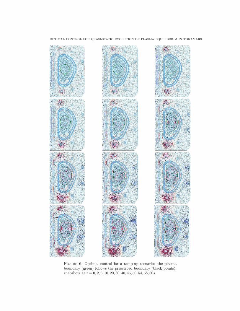
Finally, we would like to show first results for a so-called ramp-up scenario, wherethe plasma evolves from a small circular to a large elongated plasma. We simulate60s. The computed coil voltages are depicted in Figure 5. Then, if we use thoseas data to solve the direct problem we observe that the plasma boundary followsindeed the prescribed trajectory (see Figure 6).

5. Conclusions and Perspectives

The models that describe the evolution of plasma in tokamak devices are highlynon-linear. Already a direct simulation, meaning a simulation that shows onlyhow the plasma will evolve for certain given control inputs is a demanding task.


Figure 4. Dynamic free-plasma-boundary problem: the plasmaboundary (magenta) follows the prescribed boundary (whitepoints).

Figure 5. Instationary Equilibrium: The optimal voltages.

Elongated plasmas are known to suffer from serious physical instabilities [23, Section6.15], and therefore also numerical methods will be very likely to be unstable.

On the other hand, the real pivotal question for the control of plasma is thetask to find those control parameters that ensure that the plasma evolves throughcertain prescribed states. From the engineering point of view it would be beneficialto provide the majority of control as feed-forward control that can be determined apriori, and to minimize the amount of feed-back control that needs to be calculatedduring the operation. Until today, the calculation of the feed-forward control ismainly tackled by linear ODE models that have the flavor of electrical circuits.These ODE models determine the coil voltages that correspond to the coil currentsof precomputed static equilibria. Particular feed-back controller are then necessaryto ensure that the currents in the system are indeed close to the precomputed ones.The utility of this approach is underlined by the fact that control engineers havetoday the knowledge to operate the present tokamaks.

Nevertheless we believe that the computation of feed-forward control can be donemuch more accurately. In this work we formulated an optimal control problem, thatuses the force balance (1) and Maxwell’s equations (2) as constraints, to computedirectly the optimal feed-forward control. This approach is much more consistent,since we use the full nonlinear PDE model. Then, in the solution of this optimiza-tion problem, it is Newton’s method that determines consistently the linearization,that provide the linear approximation of the non-linear model.


Figure 6. Optimal control for a ramp-up scenario: the plasmaboundary (green) follows the prescribed boundary (black points),snapshots at t = 0, 2, 6, 10, 20, 30, 40, 45, 50, 54, 58, 60s.


We presented here the two basic ingredients, the finite element method and se-quential quadratic programming, to set up such an optimal control approach forplasma evolution in tokamaks. The finite element method allows for an easy treat-ment of free plasma boundary and the decaying conditions at infinity. Further, wecan, almost automatically, compute linearizations and the adjoint operators thatare required for the optimization with sequential quadratic programming. In thefuture we will have to augment the non-linear model (3)-(6) with further equations,namely the resitive diffusion and transport equations, that provide a more com-plete description. Our preliminary simulations provide a fairly promising proof ofconcepts.

References

[1] R. Albanese, J. Blum, and O. Barbieri. On the solution of the magneticflux equation in an infinite domain. In EPS. 8th Europhysics Conference onComputing in Plasma Physics (1986), 1986.

[2] M. Ariola and A. Pironti. Magnetic Control of Tokamak Plasmas. SpringerLondon, 2008.

[3] J. Blum. Numerical simulation of the plasma equilibrium in a tokamak.Wiley/Gauthier-Villars, 1987.

[4] J. Blum and J. Le Foll. Plasma equilibrium evolution at the resistive diffusiontimescale. Computer Physics Reports, 1(7-8):465–494, 1984.

[5] J. Blum, J. Le Foll, and B. Thooris. The self-consistent equilibrium and diffu-sion code SCED. Computer Physics Communications, 24:235 – 254, 1981.

[6] J.A. Crotinger. Corsica; a comprehensive simulation of toroidal magnetic-fusion devices. Technical report ucrl-id-126284, Lawrence Livermore NationalLaboratory, 1997.

[7] E. Fable, C. Angioni, A. A. Ivanov, K. Lackner, O. Maj, S. Yu, Medvedev,G. Pautasso, and G. V. Pereverzev. A stable scheme for computation of coupledtransport and equilibrium equations in tokamaks. Nuclear Fusion, 53(3), 2013.

[8] J. P. Freidberg. Ideal Magnetohydrodynamics. Plenum US, 1987.[9] G.N. Gatica and G.C. Hsiao. The uncoupling of boundary integral and finite

element methods for nonlinear boundary value problems. J. Math. Anal. Appl.,189(2):442–461, 1995.

[10] H. Grad and J. Hogan. Classical diffusion in a tokomak. Phys. Rev. Lett.,24:1337–1340, Jun 1970.

[11] H. Grad, P. N. Hu, and D. C. Stevens. Adiabatic evolution of plasma equilib-rium. Proc Natl Acad Sci U S A., 72:3789–3793, 1975.

[12] H. Grad and H. Rubin. Hydromagnetic equilibria and force-free fields. Pro-ceedings of the 2nd UN Conf. on the Peaceful Uses of Atomic Energy, 31:190,1958.

[13] Virginie Grandgirard. Modelisation de l’equilibre d’un plasma de tokamak.PhD thesis, l’Universite de Franche-Comte, 1999.

[14] M. Hinze, R. Pinnau, M. Ulbrich, and S. Ulbrich. Optimization with PDEconstraints, volume 23 of Mathematical Modelling: Theory and Applications.Springer, New York, 2009.

[15] M. Honda. Simulation technique of free-boundary equilibrium evolution inplasma ramp-up phase. Computer Physics Communications, 181(9):1490–1500, SEP 2010.


[16] A. A. Ivanov, R. R. Khayrutdinov, S. Yu. Medvedev, and Yu. Yu Poshekhonov.The SPIDER code - solution of direct and inverse problems for free boundarytokamak plasma equilibrium. Technical Report 39, Keldysh Institute, 2009.

[17] Stephen Jardin. Computational methods in plasma physics. Boca Raton, FL :CRC Press/Taylor & Francis, 2010.

[18] K. Lackner. Computation of ideal MHD equilibria. Computer Physics Com-munications, 12(1):33 – 44, 1976.

[19] R. Lust and A. Schluter. Axialsymmetrische magnetohydrodynamische Gle-ichgewichtskonfigurationen. Z. Naturforsch. A, 12:850–854, 1957.

[20] J.L. Luxon and B.B. Brown. Magnetic analysis of non-circular cross-sectiontokamaks. Nuclear Fusion, 22(6):813, 1982.

[21] J. Nocedal and S. J. Wright. Numerical optimization. Springer Series in Opera-tions Research and Financial Engineering. Springer, New York, second edition,2006.

[22] V. D. Shafranov. On magnetohydrodynamical equilibrium configurations. So-viet Journal of Experimental and Theoretical Physics, 6:545, 1958.

[23] J. Wesson. Tokamaks. The International Series of Monographs in Physics.Oxford University Press, 2004.

E-mail address: [email protected]

CASTOR TEAM, INRIA, 2004, Route des Lucioles, BP 93, 06560 Sophia Antipolis,

France

E-mail address: [email protected]

Laboratoire J.-A. Dieudonne, Universite de Nice, Parc Valrose, 06108 Nice cedex

2, France & CASTOR TEAM, INRIA, 2004, Route des Lucioles, BP 93, 06902 Sophia

Antipolis, France

optimal control for quasi-static evolution of plasma

Documents