optimal consumption and savings with stochastic …optimal consumption and savings with stochastic...

Optimal consumption and savings withstochastic income∗

Chong Wang† Neng Wang‡ Jinqiang Yang§

August 6, 2013

Abstract

We develop an analytically tractable consumption-savings model for a liquidity-constrained agent who faces both permanent and transitory income shocks. We findthat risk aversion and intertemporal substitution have very different effects on bothconsumption and the steady-state savings target. Moderate changes in risk aversionhave large effects on consumption and buffer-stock savings. With permanent shocks,it takes many years to reach the steady-state savings target. We also find that largediscrete income shocks (jumps) occurring at low frequencies can be very costly. Unlikeconventional wisdom, transitory shocks can generate very large precautionary savingsdemand, especially for low transitory income states.

Keywords: buffer stock; precautionary savings; incomplete markets; borrowing con-straints; income fluctuations; permanent income; transitory income; jumps; non-expectedutility

JEL Classification: E2

∗We thank Mark Gertler, Pierre-Olivier Gourinchas, Lars Hansen, Bob Hodrick, Erik Hurst, Dirk Krueger,Fabrizio Perri, Tom Sargent, Suresh Sundaresan, Steve Zeldes, and seminar participants at Columbia andSUFE for helpful comments.†Graduate School of Business and Public Policy, Naval Postgraduate School. Email: [email protected].‡Columbia Business School, NBER, and SUFE. Email: [email protected].§Shanghai University of Finance and Economics (SUFE). Email: [email protected].

1 Introduction

Income shocks fundamentally influence households’ consumption and savings decisions espe-

cially when markets offer limited opportunities for households to manage these uninsurable

permanent or transitory income risks. Households often find it hard to borrow against their

future incomes due to various frictions including informational asymmetry, agency conflicts,

and limited enforcement just to name a few. What is the impact of borrowing constraints on

consumption and wealth accumulation? How do income shocks, such as large discrete income

shocks (e.g. unemployment), or continuous diffusive income shocks influence consumption

and savings policies? What are the effects of intertemporal substitution and risk aversion

on consumption and steady-state target savings?

We address these important questions by developing an analytically tractable dynamic

incomplete-markets model with the following important new features. First, we choose the

non-expected recursive utility developed by Epstein and Zin (1989) and Weil (1990), as we

show that the distinction between risk aversion and intertemporal substitution is critically

important for us to understand dynamic consumption-savings behavior, both qualitatively

and quantitatively.1 Second, our model allows us to tractably incorporate empirically and

quantitatively important income processes with (a) permanent and transitory shocks, (b) dif-

fusive/continuous and discrete/jump shocks, and (c) mean-reverting income growth shocks.

Third, our model has important quantitative implications on the convergence and the steady-

state savings target. For example, our model allows us to study how different structural

parameters (e.g. risk aversion and intertemporal substitution) influence the short-run and

long-run savings behavior.

Our continuous-time model allows us to analytically characterize the optimal consump-

tion policy and the welfare measure (the certainty equivalent wealth) by using (1) an ordi-

nary differential equation (ODE), (2) a first-order condition (FOC) for consumption, and

(3) intuitive boundary conditions, all implied by the agent’s optimality. These three parts

complement each other by providing different but important and intuitive economic insights

to our understanding of the savings behaviors. Specifically, by exploiting the homogeneity

property of our model as in the discrete-time expected isoelastic utility formulation of Carroll

1Recursive utility that separates risk aversion from intertemporal substitution has become a standardpractice in the asset pricing literature. See the long-run risk literature pioneered by Bansal and Yaron(2004). The application of this class of utility is less common in the consumption-savings literature.

1

(1997), we characterize the optimal consumption policy and the value function via the “ef-

fective” state variable, the wealth-income ratio w. This ratio w captures the liquid financial

wealth per unit of income. The larger this liquidity measure w, the less financially con-

strained the agent. Unlike existing work, we characterize the optimal consumption-income

ratio c(w) explicitly up to a tractable nonlinear ordinary differential equation (ODE), which

we can solve with very high numerical precision with no need for log-linearization. Our

model shows that the consumption rule is highly nonlinear as a function of liquidity w.

Simply applying log-linearization to our model is highly undesirable and will lose important

state-contingent nonlinear consumption dynamics. Although the financial constraint rarely

binds in the model, it can still be very costly. Anticipating the low-probability but high-cost

scenario, financial constraints have significant effects on savings even when the agent has

moderate levels of liquidity w. The analytical consumption rule is intuitive and links to

the agent’s welfare measure (certainty equivalent wealth) and the marginal value of liquid-

ity. The boundary condition (at the moment when the agent runs out of liquidity/savings)

naturally reflects whether the liquidity constraint binds or not, and the boundary condi-

tion (when liquidity is abundant) naturally corresponds to the complete-markets frictionless

permanent-income hypothesis result.

One main result is that intertemporal substitution and risk aversion have fundamentally

different effects on both consumption and buffer-stock savings behavior. Changing the co-

efficient of relative risk aversion (e.g. from two to four) leads to a quantitatively enormous

increase of buffer-stock savings. For example, in our baseline calculation, as we increase risk

aversion from 2 to 4, the steady-state target for the wealth-income ratio increases signifi-

cantly from 2.6 to 16. In contrast to the conventional view, even for transitory income shocks,

precautionary savings demand can be very large for low values of liquidity w; The optimal

consumption rule is highly nonlinear and standard linear-quadratic approximations may not

capture the richness of consumption dynamics. We also find that a rational consumer with

no liquid wealth may voluntarily choose to live from paycheck to paycheck (e.g. hand-to-

mouth) with no savings, which is consistent with the findings in Campbell and Mankiw

(1989). Finally, the convergence to the buffer-stock savings target often takes a very long

time (e.g. one hundred years) for an agent starting with no wealth.

Related Literature. Hall (1978) formalizes Friedman’s seminal permanent-income hy-

2

pothesis via the martingale (random-walk) consumption in a dynamic programming frame-

work.2 Zeldes (1989) and Deaton (1991) numerically solve the optimal consumption rule for

expected constant relative risk averse (CRRA) utility. Carroll (1997) notes the importance

of impatience and develops buffer-stock savings models for expected CRRA utility.3 The

dominant paradigm in the consumption literature is the isoelastic utility based models as

wealth effects are important for consumption decisions.

There is a smaller literature in consumption that tries to derive tractable and intuitive

consumption rules that capture important economic insights. These models tend to rely on

constant absolute risk averse (CARA) utility, which rules out the wealth effect. Caballero

(1990, 1991) solve the optimal consumption and saving rules in closed form by assuming

CARA utility and conditionally homoskedastic (autoregressive and moving average) labor-

income processes. To show how missing markets and uninsurable income shocks invalidate

the Ricardian equivalence, Kimball and Mankiw (1989) also use CARA utility and obtain

an effectively explicit consumption rule with a two-state Markov chain for the income in an

incomplete-markets setting. Wang (2006) generalizes the conditionally homoskedastic labor-

income process in Caballero (1991) to allow for conditional heteroskedasticity4 and obtains a

closed-form optimal consumption rule. Unlike Caballero (1991) where precautionary savings

demand is constant and the MPC out of human wealth equals that out of financial wealth,

Wang (2006) finds stochastic precautionary savings and the MPC out of human wealth

to be lower than that out of financial wealth due to the conditional heteroskedasticity of

labor-income shocks. In these CARA-utility-based models, for tractability reasons, liquidity

constraints are not imposed. Unlike these CARA-utility-based models, our model has both

uninsurable shocks and liquidity constraints.

Finally, we note that Weil (1993) solves a discrete-time precautionary-saving model in

closed form under the assumption of a non-expected utility with CARA and a constant

2For early important contributions on consumption and savings in stochastic settings, see Leland (1968),Levhari and Srinivasan (1969), Sandmo (1970), and Dreze and Modigliani (1972), among others. Deaton(1992) and Attanasio (1999) survey the literature.

3For more recent work on optimal consumption and savings, see Gourinchas and Parker (2002), Storeslet-ten, Telmer, and Yaron (2004), Aguiar and Hurst (2005), Guvenen (2006, 2007), Fernandez-Villaverde andKrueger (2007), and Kaplan and Violante (2010), among others.

4In Wang (2006), the conditional variance of income changes is an affine function in the current laborincome level. This affine labor-income process is widely used in the finance literature, e. g. the termstructure of interest rates. See Cox, Ingersoll, and Ross (1985) for a seminal contribution and Duffie (2001)for an introductory textbook treatment on “affine” models in finance.

3

elasticity of intertemporal substitution (EIS). He also finds a constant precautionary savings

demand as Caballero (1990, 1991) due to the assumption of atemporal CARA utility. Our

work shares the focus with Weil (1993) on recursive utility, but we use the more plausible

atemporal CRRA utility and generate a stochastic precautionary savings demand. The

choice of the atemporal CARA utility partly explains why Weil (1993) obtains an explicit

consumption rule, whereas we obtain the optimal consumption policy in closed form up to

an ODE with appropriate boundary conditions.

2 Model

We consider a continuous-time environment where an infinitely-lived agent receives an ex-

ogenously given perpetual stream of stochastic labor income. The agent saves via a risk-free

asset that pays interest at a constant rate r > 0. There exist no other financial assets. Addi-

tionally, liquid financial wealth is not allowed to be negative. Hence, markets are incomplete

with respect to labor-income shocks.

A typical specification of a labor-income process in the literature involves both permanent

and transitory shocks.5 For expositional convenience, we first specify the labor income

process Y as one with permanent shocks only and leave the generalization of the labor-

income process with both permanent and transitory shocks to Section 7. For simplicity, we

first consider the following widely used labor-income process specification:

dYt = µYtdt+ σYtdBt , Y0 > 0 , (1)

where B is a standard Brownian motion, µ is the expected income growth rate, and σ

measures income growth volatility. The labor-income process (1) implies that the growth

rate of income, dYt/Yt, is independently, and identically distributed (i.i.d.).

We may also write the dynamics for logarithmic income, lnY , by using Ito’s formula as,

d lnYt =(µ− σ2/2

)dt+ σdBt . (2)

Equation (2) is an arithmetic Brownian motion, which implies that lnY is a unit-root process.

The change of income ∆ lnY has mean (µ− σ2/2) and volatility σ per unit of time. While

income shocks are i.i.d. for the income growth rate, they are permanent in levels of Y .

5See MaCurdy (1982), Abowd and Card (1989), and Meghir and Pistaferri (2004), for example. Givenour focus, we also ignore life-cycle variations and various fixed effects including education and gender.

4

The widely-used standard preference in the consumption/savings literature is the ex-

pected utility with constant relative risk aversion, which ties the elasticity of intertemporal

substitution (EIS) to the inverse of the coefficient of relative risk aversion. Conceptually, risk

aversion and the EIS are fundamentally different and have different effects on consumption-

savings decisions. We thus use the non-expected recursive utility developed by Epstein and

Zin (1989) and Weil (1990), who build on Kreps and Porteous (1978), which allows econom-

ically meaningful separation between risk aversion and the EIS. Specifically, the preference

features both a constant coefficient of relative risk aversion and a constant EIS. We use the

continuous-time formulation of this non-expected utility developed by Duffie and Epstein

(1992a), and specify the recursive utility process V as follows,

Vt = Et

[∫ ∞t

f(Cu, Vu)du

], (3)

where f(C, V ) is known as the normalized aggregator for consumption C and utility V .

Duffie and Epstein (1992a) show that f(C, V ) for this recursive utility is given by

f(C, V ) =ρ

1− ψ−1

C1−ψ−1 − ((1− γ)V )θ

((1− γ)V )θ−1, (4)

and

θ =1− ψ−1

1− γ. (5)

Here, ψ is the EIS, γ is the coefficient of relative risk aversion, and ρ is the subjective discount

rate. The widely used time-additive separable CRRA utility is a special case of the recursive

utility where the coefficient of relative risk aversion γ equals the inverse of the EIS, γ = ψ−1

implying θ = 1. For the expected utility special case, we thus have f(C, V ) = U(C) − ρV ,

which is additively separable in C and V , with U(C) = ρC1−γ/(1 − γ). For the general

specification of the recursive utility, θ 6= 1 and f(C, V ) is non-separable in C and V .

The agent’s liquid financial wealth W accumulates as follows

dWt = (rWt + Yt − Ct)dt, t ≥ 0 . (6)

We assume that the agent cannot borrow against future incomes, i.e. liquid financial wealth

is non-negative at all times,

Wt ≥ 0, for all t ≥ 0 . (7)

5

Despite being unable to borrow, the agent adjusts the rate of wealth accumulation/de-

cumulation and uses liquid wealth to partially smooth consumption over time.

In summary, the agent maximizes the non-expected recursive utility given in (3)-(4)

subject to the labor-income process (1), the wealth accumulation process (6), and the non-

negative wealth constraint (7). To illustrate economic intuition in our incomplete markets

model, we first present the complete-markets (CM) benchmark and summarize its solution.

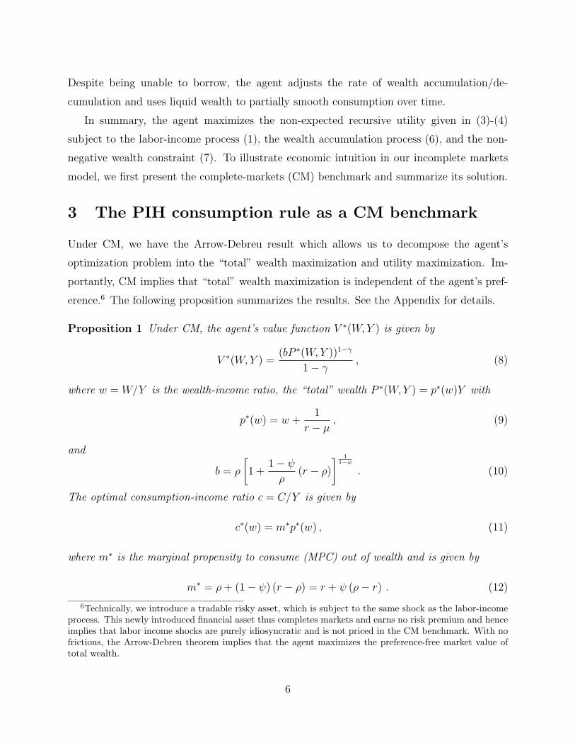
3 The PIH consumption rule as a CM benchmark

Under CM, we have the Arrow-Debreu result which allows us to decompose the agent’s

optimization problem into the “total” wealth maximization and utility maximization. Im-

portantly, CM implies that “total” wealth maximization is independent of the agent’s pref-

erence.6 The following proposition summarizes the results. See the Appendix for details.

Proposition 1 Under CM, the agent’s value function V ∗(W,Y ) is given by

V ∗(W,Y ) =(bP ∗(W,Y ))1−γ

1− γ, (8)

where w = W/Y is the wealth-income ratio, the “total” wealth P ∗(W,Y ) = p∗(w)Y with

p∗(w) = w +1

r − µ, (9)

and

b = ρ

[1 +

1− ψρ

(r − ρ)

] 11−ψ

. (10)

The optimal consumption-income ratio c = C/Y is given by

c∗(w) = m∗p∗(w) , (11)

where m∗ is the marginal propensity to consume (MPC) out of wealth and is given by

m∗ = ρ+ (1− ψ) (r − ρ) = r + ψ (ρ− r) . (12)

6Technically, we introduce a tradable risky asset, which is subject to the same shock as the labor-incomeprocess. This newly introduced financial asset thus completes markets and earns no risk premium and henceimplies that labor income shocks are purely idiosyncratic and is not priced in the CM benchmark. With nofrictions, the Arrow-Debreu theorem implies that the agent maximizes the preference-free market value oftotal wealth.

6

Friedman (1957) and Hall (1978) define human wealth H as the expected present value

of future labor income, discounted at the risk-free interest rate r, in that

Ht = Et

(∫ ∞t

e−r(u−t)Yudu

). (13)

With CM and idiosyncratic labor income risk, human wealth H defined by (13) then gives

the market value of income. With r > µ, human wealth H is finite and is given by

Ht = hYt =Yt

r − µ. (14)

The total wealth per unit of income is given by the sum of w and h, p∗(w) = w+ h, and the

optimal consumption-income ratio is given by c∗ = m∗ (w + h). Next, we characterize the

solution for the case where the agent faces both the borrowing constraint and uninsurable

shocks.

4 Solution: The Incomplete-Markets Setting

We proceed in two steps. First, we analyze the agent’s consumption policy rule in the

interior region with positive wealth, i.e. Wt > 0, and then discuss the boundary conditions.

In the interior region, the agent chooses consumption to satisfy the Hamilton-Jacobi-Bellman

(HJB) equation,7

0 = maxC>0

f(C, V ) + (rW + Y − C)VW (W,Y ) + µY VY (W,Y ) +σ2Y 2

2VY Y (W,Y ) .(15)

The first-order condition (FOC) for consumption is given by

fC(C, V ) = VW (W,Y ) , (16)

which equates the marginal benefit of consumption fC(C, V ) with the marginal value of

wealth VW (W,Y ). For the special CRRA utility case, fC(C, V ) equals the marginal utility

of consumption U ′(C), which is independent of the agent’s continuation value V . More

generally, for a non-expected utility, fC(C, V ) depends on both current consumption C and

the agent’s continuation value V , as f(C, V ) is not additively separable in C and V .

7Duffie and Epstein (1992b) generalize the standard HJB equation for the expected-utility case, to allowfor non-expected recursive utility such as the Epstein-Weil-Zin utility used here.

7

We show that the agent’s value function is given by

V (W,Y ) =(bP (W,Y ))1−γ

1− γ, (17)

where b is given by (10). By comparing the value function V (W,Y ) given in (17) with

V ∗(W, 0) given by (8) for the CM benchmark with no labor income, we refer to P (W,Y )

as the certainty equivalent wealth, the minimal amount of wealth for which the agent is

willing to permanently give up the labor income process Y and liquid wealth W , V (W,Y ) =

V ∗(P (W,Y ), 0).

With the homothetic recursive utility and a geometric labor-income process, our model

has the homogeneity property as the expected CRRA utility does.8 We use the lower case

to denote the corresponding variable in the upper case scaled by contemporaneous labor

income Y . For example, wt = Wt/Yt denotes the wealth-income ratio, ct = Ct/Yt is the

consumption-income ratio, and p(w) = P (W,Y )/Y is the scaled certainty equivalent wealth.

The following theorem summarizes the main results and the details are provided in the

Appendix.

Theorem 1 With incomplete markets, the consumption-income ratio c(w) is given by

c(w) = m∗p(w)(p′(w))−ψ, (18)

where m∗ as given in (12) is the agent’s MPC under CM and the scaled certainty equivalent

wealth p(w) solves the following ordinary differential equation (ODE):

0 =

(m∗(p′(w))1−ψ − ψρ

ψ − 1+ µ− γσ2

2

)p(w) + p′(w) + (r − µ+ γσ2)wp′(w)

+σ2w2

2

(p′′(w)− γ (p′(w))2

p(w)

). (19)

The above ODE for p(w) is solved subject to the following conditions:

limw→∞

p(w) = p∗(w) = w + h = w +1

r − µ, (20)

0 =

(m∗(p′(0))1−ψ − ψρ

ψ − 1+ µ− γσ2

2

)p(0) + p′(0) . (21)

Additionally, the ODE (19) for p(w) satisfies the following constraint for c( · ) at the origin,

0 < c(0) ≤ 1 . (22)

8Carroll (1997) shows the homogeneity property for the CRRA utility case and numerically solves for theoptimal consumption rule in the discrete-time setting.

8

The optimal consumption rule c(w) depends on both the scaled certainty equivalent

wealth p(w) and its slope p′(w), the marginal (certainty equivalent) value of wealth. Frictions

(uninsurable labor income shocks and the borrowing constraint) cause p(w) to be highly non-

linear. First, the frictions lower the certainty equivalent wealth p(w) from its first-best CM

value p∗(w) = w + h. Second, the frictions cause the marginal value of wealth p′(w) to be

greater than unity, p′(w) > 1. Therefore, consumption c(w) given by (18) is lower than the

CM benchmark level, c(w) < c∗(w), as p(w) < w + h and p′(w) ≥ 1.

The ODE (19) describes the nonlinear certainty equivalent valuation p(w) in the interior

region w > 0. In the limit as w → ∞, wealth completely buffers labor income shocks.

Therefore, limw→∞ p(w) = w + h, limw→∞ p′(w) = 1 , and limw→∞ c(w) = m∗(w + h). This

CM result in the limit serves as one natural boundary condition for the ODE (19). At the

left boundary, w = 0, the condition is given by (21), which is the limit of the ODE (19).

In our continuous-time formulation, we need only check whether the borrowing constraint

Wt ≥ 0 binds or not at the boundary (i.e. when w = 0) and not in the interior region (i.e.

when w > 0) as consumption is a “flow” variable and wealth is a “stock” variable. Therefore,

any consumption flow over an infinitesimal time period is feasible provided that wealth is

positive, w > 0. This property makes our continuous-time model analysis more tractable

than the standard discrete-time analysis.

Note that the borrowing constraint Wt ≥ 0 is equivalent to the consumption constraint

at the origin, c(0) ≤ 1 which is given by (22).9 This inequality and the condition (21) jointly

characterize the left boundary for the ODE (19). Optimal consumption is characterized by

one of the two sub-cases: c(0) = 1 and c(0) < 1.

If c(0) = 1, the constraint W ≥ 0 binds permanently after wealth reaches zero. At W = 0,

the agent permanently saves nothing and hence behaves as a “hand-to-mouth” consumer.

Campbell and Mankiw (1989) find that about 50% of households in their sample do not save.

We show that these consumers’ behavior can be optimal in our model. For “hand-to-mouth”

consumers, relaxing the borrowing constraint can cause the consumption profile to change

and hence can be welfare-enhancing.

In contrast, if c(0) < 1, the borrowing constraint W ≥ 0 never binds. In this case,

relaxing the borrowing constraint (e.g. by offering a credit line) has no effect on optimal

9Suppose Wt− = 0. Then, wealth evolution is simply given by dWt = (Yt − Ct)dt, and consumption Ct

thus cannot to exceed income Yt, i.e. c(wt−) ≤ 1 is necessary when wt− = 0.

9

consumption and savings, as the precautionary savings demand is sufficiently high and the

agent optimally chooses consumption in such a way that wealth always remains positive

with probability one. Intuitively, running the risk of exhausting all savings with any positive

probability is not optimal.

Technically, the optimal consumption c(w) and the certainty equivalent wealth p(w)

jointly solve the FOC (18) and the ODE (19) subject to the boundary conditions (20)-(21)

and the borrowing constraint (22).

5 Results

We now analyze our model’s predictions on consumption, savings, and the long-run station-

ary distributions for scaled wealth and consumption. Parameter values are annualized and

continuously compounded when applicable. We set the subjective discount rate ρ = 5.5%

and the risk-free rate r = 5%, which imply that the agent is relatively impatient (compared

with the market), with a wedge ρ − r = 0.5%. In general, our model does not require

ρ > r. We choose the expected income growth rate µ = 1%, the volatility of income growth

σ = 10%, and the EIS parameter ψ = 0.5. We consider three values for the coefficient of rel-

ative risk aversion, γ = 0, 2, 4 and we will show that the quantitative effects of risk aversion

on consumption and welfare are large. The case with γ = 2 corresponds to the expected

CRRA utility with ψ = 1/γ = 0.5. The case with risk neutrality (γ = 0) and a positive EIS

is proposed by Farmer (1990) and used by Gertler (1999) in his study of social security in a

life-cycle economy.

5.1 Optimal consumption and certainty equivalent wealth

Panels A and B of Figure 1 plot p(w) and p′(w), respectively. Uninsurable labor income

shocks and the borrowing constraint cause p(w) to be concave in w. Because wealth buffers

labor-income shocks and mitigates the impact of the borrowing constraint on consumption,

the marginal (certainty equivalent) value of liquid wealth p′(w) is greater than one. In-

tuitively, p′(w) decreases with w, as a wealthier agent is less concerned about uninsurable

labor-income shocks and the borrowing constraint, ceteris paribus. As w →∞, incomplete-

markets frictions no longer matter, and hence p′(w) approaches one. Next, we turn to the

consumption rule, c(w), and the MPC, c′(w). Panels C and D of Figure 1 plot c(w) and

10

0 5 10 15 2015

20

25

30

35

40

45A. scaled certainty equivalent wealth p(w)

wealth−income ratio w

!=0!=2!=4

0 5 10 15 201

1.1

1.2

1.3

1.4

1.5

1.6B. marginal value of wealth p"(w)


0 5 10 15 200.8

1

1.2

1.4

1.6

1.8

2

2.2

C. consumption−income ratio c(w)

wealth−income ratio w0 5 10 15 20

0.05

0.1

0.15

0.2

0.25

0.3

0.35

0.4D. MPC out of wealth c"(w)


Figure 1: Scaled certainty equivalent wealth p(w), marginal (certainty equivalent)value of wealth p′(w), optimal consumption-income ratio c(w), and the MPC outof wealth c′(w). Parameter values are: r = 5%, ρ = 5.5%, σ = 10%, µ = 1%, and ψ = 0.5.

the MPC out of wealth, c′(w), respectively, and show that consumption is increasing and

concave in wealth.10

The risk-neutral agent (γ = 0) withW = 0 values a unit of windfall wealth at p′(0) = 1.53,

which is 53% higher than its face value. The agent with no wealth consumes all labor income,

c(0) = 1, and wealth is permanently absorbed at W = 0. The MPC out of wealth at W = 0

is c′(0) = 36.6%, which is much higher than the CM benchmark value m∗ = 0.0525 and

reflects the significant cost of the borrowing constraint. With risk neutrality, γ = 0, the

marginal value of wealth p′(0) is greater than one, if and only if the agent is constrained and

10Carroll and Kimball (1996) show that the consumption function is concave under certain conditions forthe expected-utility case.

11

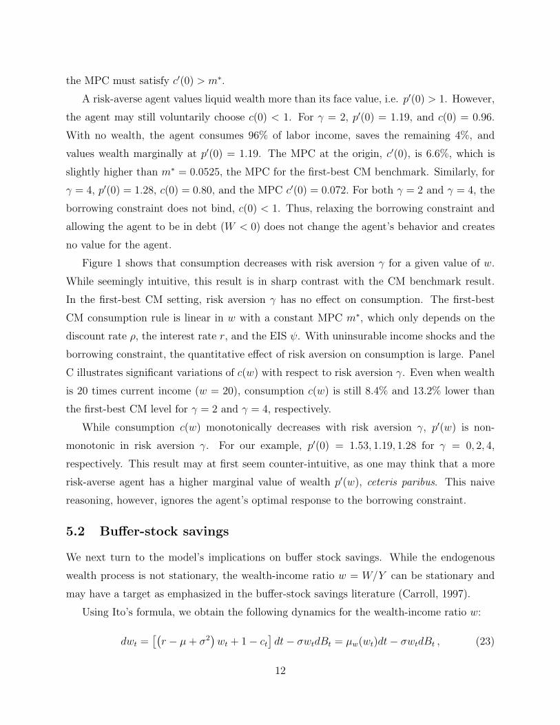
the MPC must satisfy c′(0) > m∗.

A risk-averse agent values liquid wealth more than its face value, i.e. p′(0) > 1. However,

the agent may still voluntarily choose c(0) < 1. For γ = 2, p′(0) = 1.19, and c(0) = 0.96.

With no wealth, the agent consumes 96% of labor income, saves the remaining 4%, and

values wealth marginally at p′(0) = 1.19. The MPC at the origin, c′(0), is 6.6%, which is

slightly higher than m∗ = 0.0525, the MPC for the first-best CM benchmark. Similarly, for

γ = 4, p′(0) = 1.28, c(0) = 0.80, and the MPC c′(0) = 0.072. For both γ = 2 and γ = 4, the

borrowing constraint does not bind, c(0) < 1. Thus, relaxing the borrowing constraint and

allowing the agent to be in debt (W < 0) does not change the agent’s behavior and creates

no value for the agent.

Figure 1 shows that consumption decreases with risk aversion γ for a given value of w.

While seemingly intuitive, this result is in sharp contrast with the CM benchmark result.

In the first-best CM setting, risk aversion γ has no effect on consumption. The first-best

CM consumption rule is linear in w with a constant MPC m∗, which only depends on the

discount rate ρ, the interest rate r, and the EIS ψ. With uninsurable income shocks and the

borrowing constraint, the quantitative effect of risk aversion on consumption is large. Panel

C illustrates significant variations of c(w) with respect to risk aversion γ. Even when wealth

is 20 times current income (w = 20), consumption c(w) is still 8.4% and 13.2% lower than

the first-best CM level for γ = 2 and γ = 4, respectively.

While consumption c(w) monotonically decreases with risk aversion γ, p′(w) is non-

monotonic in risk aversion γ. For our example, p′(0) = 1.53, 1.19, 1.28 for γ = 0, 2, 4,

respectively. This result may at first seem counter-intuitive, as one may think that a more

risk-averse agent has a higher marginal value of wealth p′(w), ceteris paribus. This naive

reasoning, however, ignores the agent’s optimal response to the borrowing constraint.

5.2 Buffer-stock savings

We next turn to the model’s implications on buffer stock savings. While the endogenous

wealth process is not stationary, the wealth-income ratio w = W/Y can be stationary and

may have a target as emphasized in the buffer-stock savings literature (Carroll, 1997).

Using Ito’s formula, we obtain the following dynamics for the wealth-income ratio w:

dwt =[(r − µ+ σ2

)wt + 1− ct

]dt− σwtdBt = µw(wt)dt− σwtdBt , (23)

12

where µw(w) denotes the expected change (drift) of w and is given by

µw(w) =(r − µ+ σ2

)w + 1− c(w) . (24)

Because income Y is stochastic and wealth W (earning a constant rate of return r) is locally

deterministic, the wealth-income ratio w has stochastic volatility σwt. The negative sign for

the diffusion term in (23) indicates that w decreases as income Y receives a positive shock.

How much wealth should the agent accumulate? Since W is non-stationary, we measure

the target level of savings per unit of labor-income Y in the long-run sense. Let wss denote

the steady-state wealth-income ratio. Intuitively, around the steady-state savings target for

wss, we expect that w mean reverts; the agent increases w in expectation if w lies below

the target wss, and decreases w on average if otherwise. At the steady state, the expected

change of w, µw(w), equals zero, i.e. µw(wss) = 0, which in turn implies that the steady-state

consumption-income ratio, css(w), is given by

css(w) = 1 +(r − µ+ σ2

)wss . (25)

Intuitively, the steady-state consumption per unit of income css(w) equals one plus a term

that is proportional to the steady-state savings target, wss, with coefficient (r − µ+ σ2).

This coefficient is given by the interest rate r minus the expected income growth rate µ, plus

σ2, the Jensen’s inequality term.

There are two cases, wss = 0 and wss > 0. If wss = 0, the borrowing constraint binds and

c(wss) = 1. With no initial wealth, this agent lives from paycheck to paycheck, or “hand to

mouth.” Campbell and Mankiw (1989) find that many consumers behave in this way. We

show that these consumers may behave optimally. In our numerical exercises, the case with

γ = 0 is one such example with zero steady-state savings, wss = 0.

If wss > 0, the wealth-income ratio w mean reverts. The following condition ensures that

the wealth-income ratio w is stationary:

ρ− r > −ψ−1(µ− σ2

), (26)

because limw→∞ µw(w) = limw→∞ 1+[−µ+ σ2 − ψ(ρ− r)]w < 0 under the above condition.

Equation (26) requires the agent to be sufficiently impatient.11 Interestingly, risk aversion γ

11Carroll (1997) provides a similar condition under discrete-time for the case of expected CRRA utility.

13

0 2 4 6 8 10 12 14 16 18 200.5

1

1.5

2

2.5consumption−income ration: c(w)


!wss !wss!wss

"=0"=2"=4FB(r−µ+#2)w+1

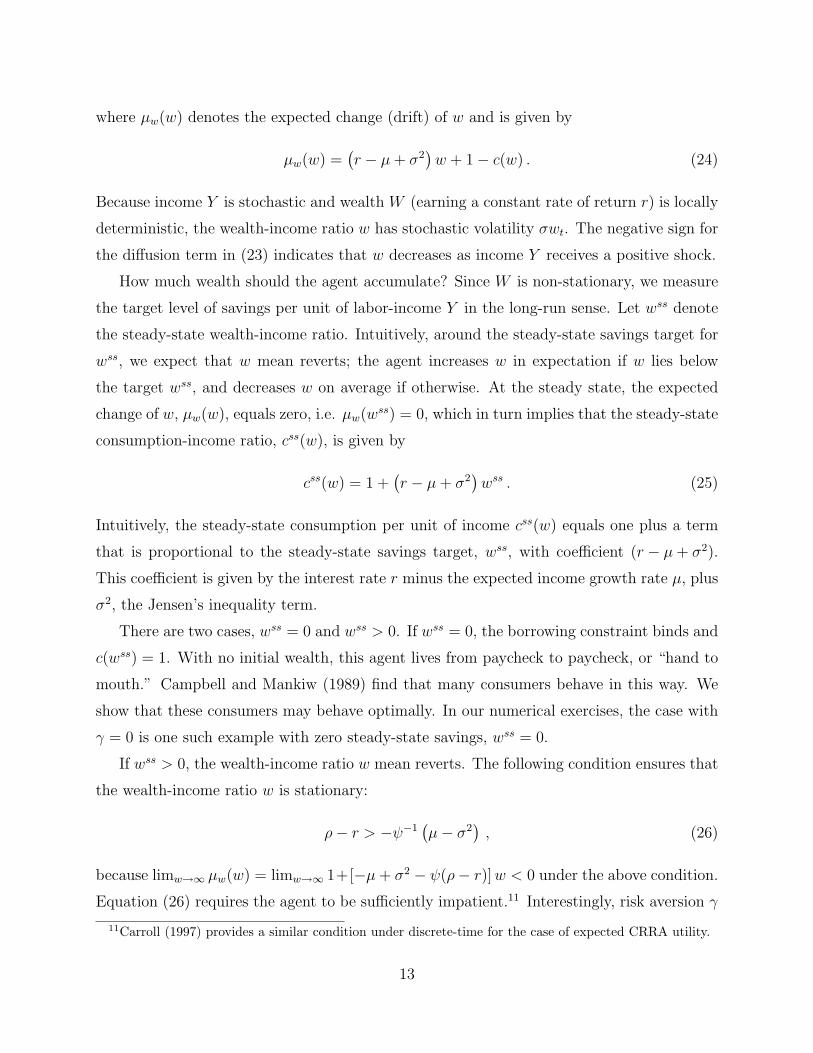
Figure 2: The steady-state wealth-income ratio wss for γ = 0, 2, 4. The steady-statewealth-income ratio wss is equal to 2.60 and 16.10 for γ = 2 and γ = 4, respectively. Forγ = 0, the steady-state wealth-income ratio is zero implying that the risk-neutral agents are“hand-to-mouth.” Parameter values are: r = 5%, ρ = 5.5%, σ = 10%, µ = 1%, and ψ = 0.5.

does not determine the stationarity of w as we see from (26). This is because in the limit,

it is the CM PIH rule that determines the agent’s optimal consumption, and risk aversion

plays no role in the CM PIH-based consumption policy. The standard impatience condition

ρ > r is neither necessary nor sufficient to ensure that w is stationary.

Figure 2 plots the optimal consumption-income ratio c(w) for γ = 0, 2, 4. As a comparison

benchmark, we also plot the first-best CM consumption rule c∗(w) = 0.0525×(w+h), which is

independent of risk aversion (see the top (dash-dotted) straight line for the PIH benchmark).

Graphically, we obtain the steady-state target wss as the intersection of the consumption

rule c(w) and the straight line (r − µ + σ2)w + 1. The steady-state target wss equals 16.10

for γ = 4, which is much higher than the savings target wss = 2.60 for γ = 2. The higher

the coefficient of relative risk aversion γ, the stronger the savings motive and the higher the

steady-state wealth-income ratio wss.

14

Table 1: The steady-state savings target wss and the distribution for thestochastic time τ to reach wss from w0 = 0.

This table reports the steady-state savings target wss and various statistics for the stochastictime τ to reach wss starting from w0 = 0 for γ = 2 and γ = 4. The EIS is ψ = 0.5 for bothcases. Various quantiles for τ are reported. For example, Prob(τ ≤ 60.8) = 25% for γ = 2.

γ wss mean std. dev. 1% 5% 25% 50% 75% 95% 99%

2 2.6 100.7 57.3 31.4 40.1 60.8 85.5 124.4 213.5 303.84 16.1 161.4 101.6 44.1 57.1 90.2 133.1 202.2 361.8 522.6

Stochastic time to reach the steady-state savings target wss from w0 = 0. Having

solved for the steady-state target wss, we next ask how long it takes for an agent with

no wealth to reach the steady-state savings target wss? Let τ denote this stochastic time,

τ = min{t : wt ≥ wss |w0 = 0}. We calculate the distribution for the stochastic time τ

via simulation. For each value of γ, we simulate two hundred thousand sample paths for

the wealth-income ratio w. Each simulation starts with w0 = 0 and terminates at the first

moment τ when wτ just equals or exceeds wss. Table 1 reports wss, the mean, standard

deviation as well as various quantile statistics for τ . The quantitative results are striking.

For an expected CRRA utility with risk aversion γ = 2, it takes on average 101 years to

build up wealth from zero to the target level wss = 2.6. The agent only has a 5% probability

of reaching the target wss = 2.6 in less than 40 years. With 25% probability, the agent will

not be able to achieve the target savings level wss even in 124 years. The results are even

more striking for γ = 4 (we keep the EIS ψ = 0.5 unchanged). The expected time to reach

the target buffer-stock savings level wss = 16.10 is 161 years. The agent only has a 1%

probability of reaching the target wss = 2.6 in less than 44 years. With 5% probability, the

agent will not be able to reach the target buffer stock savings in 362 years!

These results again suggest that incomplete-markets frictions and risk aversion have

significant effects on buffer-stock savings behavior, especially when the agent faces permanent

income shocks. While the savings target wss for γ = 4 is much higher than wss for γ = 2

(16.10 versus 2.6, which is about 6.2 times), the agent with γ = 4 also consumes less,

accumulates wealth faster, and hence the expected time to reach the savings target wss =

16.10 is only 60% longer than that the expected time to reach the savings target wss = 2.6

15

Table 2: Stationary distributions for w and c(w)

This table reports mean, standard deviation, and various quantiles for the stationary distri-butions of the wealth-income ratio w and the consumption-income ratio c(w) for γ = 2, 4.

γ mean std dev 1% 5% 25% 50% 75% 95% 99%

Panel A: w

2 3.13 2.91 0.8 1.0 1.6 2.4 3.6 7.5 13.74 18.63 19.59 4.0 5.3 8.6 12.8 21.1 57.5 171.1

Panel B: c(w)

2 1.15 0.17 1.00 1.02 1.06 1.11 1.18 1.42 1.784 1.98 1.42 1.06 1.15 1.35 1.61 2.08 4.09 10.2

for γ = 2. From the quantile statistics, we see that the distribution of the stochastic time

τ is also quite dispersed. In important early applications to macro asset pricing, Tallarini

(2000) uses a special case of the Epstein-Zin-Weil recursive utility where the elasticity on

consumption ψ = 1. He shows that the coefficient of risk aversion has significant effects on

asset market implications but limited effects on aggregate quantities in a complete-markets

production economy. Our results from the incomplete-markets single-agent’s consumption

rule reveals that the quantity implications are significant due to changes in risk aversion,

complementing his findings and indicating the importance of separating risk aversion from

the elasticity of intertemporal substitution. For applications of risk-sensitive preferences to

asset pricing, also see Hansen, Sargent, and Tallarini (1999).

5.3 Stationary distributions

We now analyze the long-run stationary distributions of w and c(w). We start from the

steady-state target wss and simulate two hundred sample paths for w by using (23). Each

path is 5,000-year long with a time increment ∆t = 0.05. Table 2 reports the mean, standard

deviation, and various quantiles for the stationary distributions of w and c(w) for γ = 2, 4.

The long-run average of w is 18.63 for γ = 4, which is about six times 3.13, the long-run

16

average of w for γ = 2. More risk-averse agents save more on average and are more likely

to be richer in the long run, consistent with our earlier findings via the steady-state savings

target wss. The long-run average of c(w) is 1.98 for γ = 4, which is 72% larger than 1.15,

the long-run average of c(w) for γ = 2. While risk aversion γ clearly also has quantitatively

significant effects on the distribution of c(w), its effects on consumption are less pronounced

than on wealth. Intuitively, more risk-averse agents accumulate more wealth to dampen the

impact of income shocks on consumption. As a more risk-averse agent accumulates more

wealth in the long run, this agent also consumes more on average.

The stationary distributions for both w and c(w) are also much more dispersed for γ = 4

than for γ = 2. Quantitatively, the effects of changing risk aversion γ from 2 to 4 on the

distributions of w and c(w) are large. Interestingly, both γ = 2 and γ = 4 are commonly

used levels of risk aversion and are sensible choices for risk aversion. However, for wealth

and consumption distributions, the quantitative results are highly sensitive to the choice of

risk aversion γ. Next, we analyze the dynamics of consumption.

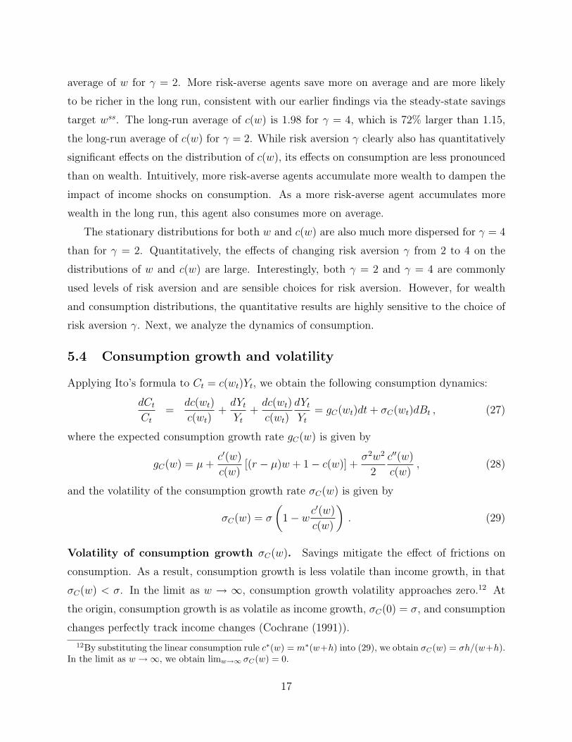
5.4 Consumption growth and volatility

Applying Ito’s formula to Ct = c(wt)Yt, we obtain the following consumption dynamics:

dCtCt

=dc(wt)

c(wt)+dYtYt

+dc(wt)

c(wt)

dYtYt

= gC(wt)dt+ σC(wt)dBt , (27)

where the expected consumption growth rate gC(w) is given by

gC(w) = µ+c′(w)

c(w)[(r − µ)w + 1− c(w)] +

σ2w2

2

c′′(w)

c(w), (28)

and the volatility of the consumption growth rate σC(w) is given by

σC(w) = σ

(1− wc

′(w)

c(w)

). (29)

Volatility of consumption growth σC(w). Savings mitigate the effect of frictions on

consumption. As a result, consumption growth is less volatile than income growth, in that

σC(w) < σ. In the limit as w → ∞, consumption growth volatility approaches zero.12 At

the origin, consumption growth is as volatile as income growth, σC(0) = σ, and consumption

changes perfectly track income changes (Cochrane (1991)).

12By substituting the linear consumption rule c∗(w) = m∗(w+h) into (29), we obtain σC(w) = σh/(w+h).In the limit as w →∞, we obtain limw→∞ σC(w) = 0.

17

0 2 4 6 8 10 12 14 16 18 20−0.01

−0.005

0

0.005

0.01

0.015

0.02

0.025

0.03

wss wss

expected consumption growth rate: gC(w)


!=0!=2!=4FB

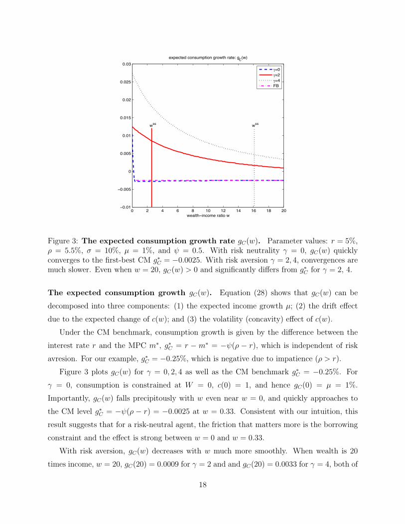
Figure 3: The expected consumption growth rate gC(w). Parameter values: r = 5%,ρ = 5.5%, σ = 10%, µ = 1%, and ψ = 0.5. With risk neutrality γ = 0, gC(w) quicklyconverges to the first-best CM g∗C = −0.0025. With risk aversion γ = 2, 4, convergences aremuch slower. Even when w = 20, gC(w) > 0 and significantly differs from g∗C for γ = 2, 4.

The expected consumption growth gC(w). Equation (28) shows that gC(w) can be

decomposed into three components: (1) the expected income growth µ; (2) the drift effect

due to the expected change of c(w); and (3) the volatility (concavity) effect of c(w).

Under the CM benchmark, consumption growth is given by the difference between the

interest rate r and the MPC m∗, g∗C = r − m∗ = −ψ(ρ − r), which is independent of risk

avresion. For our example, g∗C = −0.25%, which is negative due to impatience (ρ > r).

Figure 3 plots gC(w) for γ = 0, 2, 4 as well as the CM benchmark g∗C = −0.25%. For

γ = 0, consumption is constrained at W = 0, c(0) = 1, and hence gC(0) = µ = 1%.

Importantly, gC(w) falls precipitously with w even near w = 0, and quickly approaches to

the CM level g∗C = −ψ(ρ − r) = −0.0025 at w = 0.33. Consistent with our intuition, this

result suggests that for a risk-neutral agent, the friction that matters more is the borrowing

constraint and the effect is strong between w = 0 and w = 0.33.

With risk aversion, gC(w) decreases with w much more smoothly. When wealth is 20

times income, w = 20, gC(20) = 0.0009 for γ = 2 and and gC(20) = 0.0033 for γ = 4, both of

18

0 5 10 15 2015

20

25

30

35

40



!=0.1!=0.5!=2

0 5 10 15 201

1.05

1.1

1.15

1.2B. marginal value of wealth p"(w)


0 5 10 15 200.8

1

1.2

1.4

1.6

1.8

2

2.2



0.05

0.055

0.06

0.065

0.07

0.075



Figure 4: The effects of EIS ψ on certainty equivalent wealth and consumption.We plot p(w), p′(w), c(w), and the MPC c′(w) for ψ = 0.1, 0.5, 2. Parameter values: r = 5%,ρ = 5.5%, σ = 10%, µ = 1%, γ = 2.

which are positive and significantly different from the negative first-best CM long-run growth

rate g∗C = −0.0025. Figure 3 shows that incomplete markets frictions and risk aversion have

quantitatively important effects on consumption and wealth dynamics.

5.5 Elasticity of intertemporal substitution

We have shown that risk aversion has a first-order effect on consumption and welfare. We

next show that the EIS also matters but in a way that is quite distinct from risk aversion.

There are significant disagreements about a reasonable value for the EIS. For example,

Hall (1988) obtains an estimate of EIS near zero by using aggregate consumption data.

Bansal and Yaron (2004) show that an EIS greater than one (in the range from 1.5 to

19

2) is essential for consumption-based asset pricing models to fit empirical evidence. Thus,

choosing an EIS parameter that is larger than one has become a common practice in the

macro-finance literature. However, there is no consensus on what the sensible value of EIS

should be. The Appendix in Hall (2009) provides a brief survey of estimates in the literature.

We do not take a strong view on the value of EIS. Instead, we assess the sensitivities of

optimal consumption and welfare to changes in the EIS value from ψ = 0.1 (a low estimate

as in Hall (1988)) to ψ = 2 (a high estimate preferred by the macro finance researchers).

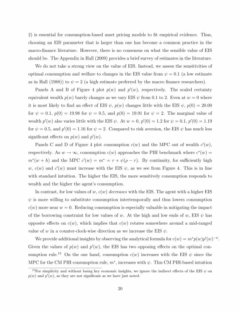
Panels A and B of Figure 4 plot p(w) and p′(w), respectively. The scaled certainty

equivalent wealth p(w) barely changes as we vary EIS ψ from 0.1 to 2. Even at w = 0 where

it is most likely to find an effect of EIS ψ, p(w) changes little with the EIS ψ, p(0) = 20.00

for ψ = 0.1, p(0) = 19.98 for ψ = 0.5, and p(0) = 19.91 for ψ = 2. The marginal value of

wealth p′(w) also varies little with the EIS ψ. At w = 0, p′(0) = 1.2 for ψ = 0.1, p′(0) = 1.19

for ψ = 0.5, and p′(0) = 1.16 for ψ = 2. Compared to risk aversion, the EIS ψ has much less

significant effects on p(w) and p′(w).

Panels C and D of Figure 4 plot consumption c(w) and the MPC out of wealth c′(w),

respectively. As w →∞, consumption c(w) approaches the PIH benchmark where c∗(w) =

m∗(w + h) and the MPC c′(w) = m∗ = r + ψ(ρ − r). By continuity, for sufficiently high

w, c(w) and c′(w) must increase with the EIS ψ, as we see from Figure 4. This is in line

with standard intuition. The higher the EIS, the more sensitively consumption responds to

wealth and the higher the agent’s consumption.

In contrast, for low values of w, c(w) decreases with the EIS. The agent with a higher EIS

ψ is more willing to substitute consumption intertemporally and thus lowers consumption

c(w) more near w = 0. Reducing consumption is especially valuable in mitigating the impact

of the borrowing constraint for low values of w. At the high and low ends of w, EIS ψ has

opposite effects on c(w), which implies that c(w) rotates somewhere around a mid-ranged

value of w in a counter-clock-wise direction as we increase the EIS ψ.

We provide additional insights by observing the analytical formula for c(w) = m∗p(w)p′(w)−ψ.

Given the values of p(w) and p′(w), the EIS has two opposing effects on the optimal con-

sumption rule.13 On the one hand, consumption c(w) increases with the EIS ψ since the

MPC for the CM PIH consumption rule, m∗, increases with ψ. This CM PIH-based intuition

13For simplicity and without losing key economic insights, we ignore the indirect effects of the EIS ψ onp(w) and p′(w), as they are not significant as we have just noted.

20

works well when the agent is effectively unconstrained, i.e. at high values of w. On the other

hand, c(w) may decrease with ψ especially for a wealth-poor (low w) agent reflected by the

term p′(w)−ψ in c(w). Intuitively, the lower the value of w, the higher the value of p′(w).

Also, the stronger the precautionary savings motive, and hence the larger the effect of the

EIS ψ. These two opposing forces imply that the comparative statics of c(w) with respect

to the EIS ψ is non-monotonic. Indeed, c(w) rotates counter-close wise as we increase the

EIS.

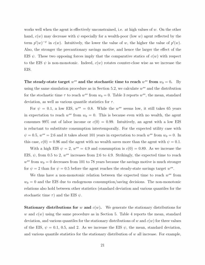
The steady-state target wss and the stochastic time to reach wss from w0 = 0. By

using the same simulation procedure as in Section 5.2, we calculate wss and the distribution

for the stochastic time τ to reach wss from w0 = 0. Table 3 reports wss, the mean, standard

deviation, as well as various quantile statistics for τ .

For ψ = 0.1, a low EIS, wss = 0.8. While the wss seems low, it still takes 65 years

in expectation to reach wss from w0 = 0. This is because even with no wealth, the agent

consumes 99% out of labor income or c(0) = 0.99. Intuitively, an agent with a low EIS

is reluctant to substitute consumption intertemporally. For the expected utility case with

ψ = 0.5, wss = 2.6 and it takes about 101 years in expectation to reach wss from w0 = 0. In

this case, c(0) = 0.96 and the agent with no wealth saves more than the agent with ψ = 0.1.

With a high EIS ψ = 2, wss = 4.9 and consumption is c(0) = 0.89. As we increase the

EIS, ψ, from 0.5 to 2, wss increases from 2.6 to 4.9. Strikingly, the expected time to reach

wss from w0 = 0 decreases from 101 to 78 years because the savings motive is much stronger

for ψ = 2 than for ψ = 0.5 before the agent reaches the steady-state savings target wss.

We thus have a non-monotonic relation between the expected time to reach wss from

w0 = 0 and the EIS due to endogenous consumption/saving decisions. The non-monotonic

relations also hold between other statistics (standard deviation and various quantiles for the

stochastic time τ) and the EIS ψ.

Stationary distributions for w and c(w). We generate the stationary distributions for

w and c(w) using the same procedure as in Section 5. Table 4 reports the mean, standard

deviation, and various quantiles for the stationary distributions of w and c(w) for three values

of the EIS, ψ = 0.1, 0.5, and 2. As we increase the EIS ψ, the mean, standard deviation,

and various quantile statistics for the stationary distribution of w all increase. For example,

21

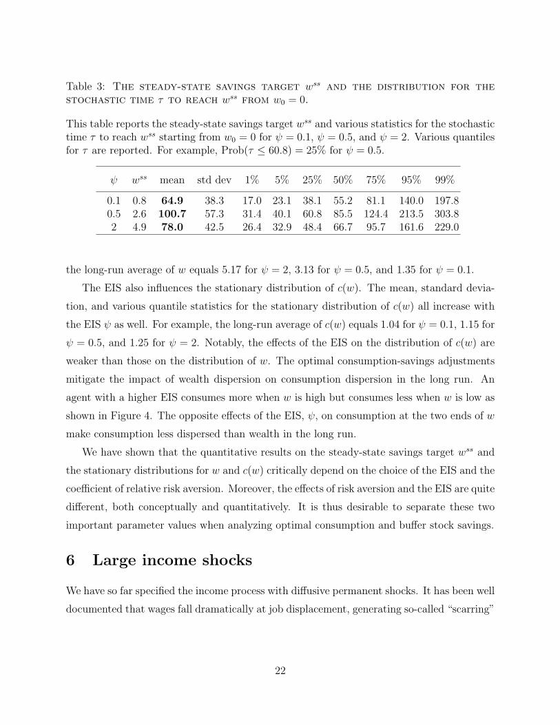
Table 3: The steady-state savings target wss and the distribution for thestochastic time τ to reach wss from w0 = 0.

This table reports the steady-state savings target wss and various statistics for the stochastictime τ to reach wss starting from w0 = 0 for ψ = 0.1, ψ = 0.5, and ψ = 2. Various quantilesfor τ are reported. For example, Prob(τ ≤ 60.8) = 25% for ψ = 0.5.

ψ wss mean std dev 1% 5% 25% 50% 75% 95% 99%

0.1 0.8 64.9 38.3 17.0 23.1 38.1 55.2 81.1 140.0 197.80.5 2.6 100.7 57.3 31.4 40.1 60.8 85.5 124.4 213.5 303.82 4.9 78.0 42.5 26.4 32.9 48.4 66.7 95.7 161.6 229.0

the long-run average of w equals 5.17 for ψ = 2, 3.13 for ψ = 0.5, and 1.35 for ψ = 0.1.

The EIS also influences the stationary distribution of c(w). The mean, standard devia-

tion, and various quantile statistics for the stationary distribution of c(w) all increase with

the EIS ψ as well. For example, the long-run average of c(w) equals 1.04 for ψ = 0.1, 1.15 for

ψ = 0.5, and 1.25 for ψ = 2. Notably, the effects of the EIS on the distribution of c(w) are

weaker than those on the distribution of w. The optimal consumption-savings adjustments

mitigate the impact of wealth dispersion on consumption dispersion in the long run. An

agent with a higher EIS consumes more when w is high but consumes less when w is low as

shown in Figure 4. The opposite effects of the EIS, ψ, on consumption at the two ends of w

make consumption less dispersed than wealth in the long run.

We have shown that the quantitative results on the steady-state savings target wss and

the stationary distributions for w and c(w) critically depend on the choice of the EIS and the

coefficient of relative risk aversion. Moreover, the effects of risk aversion and the EIS are quite

different, both conceptually and quantitatively. It is thus desirable to separate these two

important parameter values when analyzing optimal consumption and buffer stock savings.

6 Large income shocks

We have so far specified the income process with diffusive permanent shocks. It has been well

documented that wages fall dramatically at job displacement, generating so-called “scarring”

22

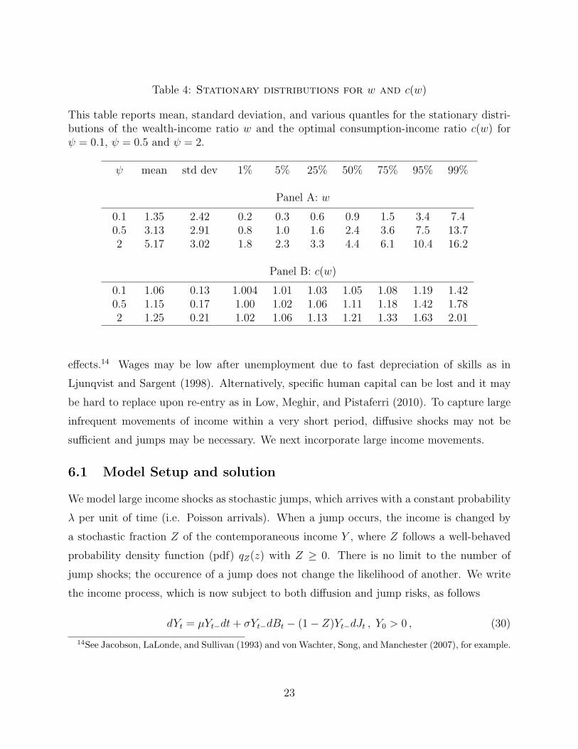
Table 4: Stationary distributions for w and c(w)

This table reports mean, standard deviation, and various quantles for the stationary distri-butions of the wealth-income ratio w and the optimal consumption-income ratio c(w) forψ = 0.1, ψ = 0.5 and ψ = 2.

ψ mean std dev 1% 5% 25% 50% 75% 95% 99%

Panel A: w

0.1 1.35 2.42 0.2 0.3 0.6 0.9 1.5 3.4 7.40.5 3.13 2.91 0.8 1.0 1.6 2.4 3.6 7.5 13.72 5.17 3.02 1.8 2.3 3.3 4.4 6.1 10.4 16.2

Panel B: c(w)

0.1 1.06 0.13 1.004 1.01 1.03 1.05 1.08 1.19 1.420.5 1.15 0.17 1.00 1.02 1.06 1.11 1.18 1.42 1.782 1.25 0.21 1.02 1.06 1.13 1.21 1.33 1.63 2.01

effects.14 Wages may be low after unemployment due to fast depreciation of skills as in

Ljunqvist and Sargent (1998). Alternatively, specific human capital can be lost and it may

be hard to replace upon re-entry as in Low, Meghir, and Pistaferri (2010). To capture large

infrequent movements of income within a very short period, diffusive shocks may not be

sufficient and jumps may be necessary. We next incorporate large income movements.

6.1 Model Setup and solution

We model large income shocks as stochastic jumps, which arrives with a constant probability

λ per unit of time (i.e. Poisson arrivals). When a jump occurs, the income is changed by

a stochastic fraction Z of the contemporaneous income Y , where Z follows a well-behaved

probability density function (pdf) qZ(z) with Z ≥ 0. There is no limit to the number of

jump shocks; the occurence of a jump does not change the likelihood of another. We write

the income process, which is now subject to both diffusion and jump risks, as follows

dYt = µYt−dt+ σYt−dBt − (1− Z)Yt−dJt , Y0 > 0 , (30)

14See Jacobson, LaLonde, and Sullivan (1993) and von Wachter, Song, and Manchester (2007), for example.

23

where J is a pure jump process. The corresponding human wealth H, as defined by (13), is

proportional to the contemporaneous income Yt, Ht = hJYt, where hJ is given by

hJ =1

r − [µ− λ(1− E(Z))]. (31)

For each realized jump, the expected percentage loss of income is (1 − E(Z)). Since jumps

occur with probability λ per unit of time, the expected income growth is thus lowered to

λ(1−E(Z)) and hence the value of labor income scaled by current Y (using the risk-free rate

to discount), hJ , is given by (31). Moreover, jumps induce precautionary savings demand

as the agent is prudent, financially constrained, and faces uninsurable jump shocks under

incomplete markets, which we can quantify using the certainty equivalent wealth.

Similar to our analysis of the baseline model, we proceed in two steps. First, we analyze

the agent’s consumption policy rule in the interior region with positive wealth, i.e. Wt >

0, and then discuss the boundary conditions. In the interior region, the agent chooses

consumption C to maximize value function V (W,Y ) by solving the following HJB equation:

0 = maxC>0

f(C, V ) + (rW + Y − C)VW + µY VY +σ2Y 2

2VY Y + λE [V (W,ZY )− V (W,Y )] .(32)

The expectation E ( · ) is with respect to QZ(z), the cumulative distribution function (cdf)

for Z. Other terms are essentially the same as those in the baseline model.

Proposition 2 The optimal consumption-income ratio c(w) is given by (18), the same as

in the baseline model. The scaled certainty equivalent wealth p(w) solves the following ODE:

0 =

(m∗(p′(w))1−ψ − ψρ

ψ − 1+ µ− γσ2

2

)p(w) + p′(w) + (r − µ+ γσ2)wp′(w)

+σ2w2

2

(p′′(w)− γ (p′(w))2

p(w)

)+

λ

1− γE

[(Zp(w/Z)

p(w)

)1−γ

− 1

]p(w) . (33)

The above ODE for p(w) is solved subject to the following conditions:

limw→∞

p(w) = w + hJ , (34)

0 =

[m∗(p′(0))1−ψ − ψρ

ψ − 1+ µ− γσ2

2+

λ

1− γE(Z1−γ − 1

)]p(0) + p′(0) . (35)

Additionally, we require 0 < c(0) ≤ 1 , the same condition as (22).

24

0 5 10 15 2015

20

25

30

35

40



!=0!=0.02!=0.05

0 5 10 15 201

1.05

1.1

1.15

1.2

1.25

1.3

1.35


B. marginal value of wealth p"(w)

0 5 10 15 20

1

1.5

2



0.06

0.07

0.08

0.09



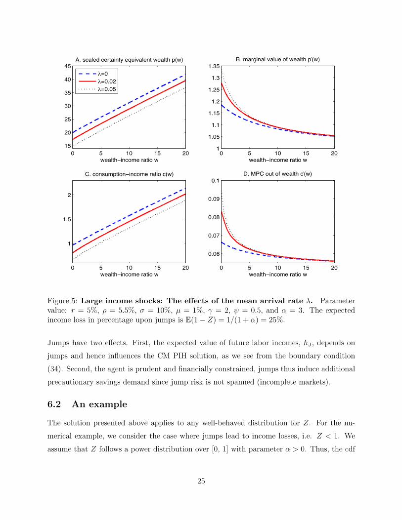
Figure 5: Large income shocks: The effects of the mean arrival rate λ. Parametervalue: r = 5%, ρ = 5.5%, σ = 10%, µ = 1%, γ = 2, ψ = 0.5, and α = 3. The expectedincome loss in percentage upon jumps is E(1− Z) = 1/(1 + α) = 25%.

Jumps have two effects. First, the expected value of future labor incomes, hJ , depends on

jumps and hence influences the CM PIH solution, as we see from the boundary condition

(34). Second, the agent is prudent and financially constrained, jumps thus induce additional

precautionary savings demand since jump risk is not spanned (incomplete markets).

6.2 An example

The solution presented above applies to any well-behaved distribution for Z. For the nu-

merical example, we consider the case where jumps lead to income losses, i.e. Z < 1. We

assume that Z follows a power distribution over [0, 1] with parameter α > 0. Thus, the cdf

25

is QZ(z) = zα and the corresponding pdf is

qZ(z) = αzα−1, 0 ≤ z ≤ 1 . (36)

A large value of α implies a small expected income loss of E(1−Z) = 1/(α+1) in percentages.

For α = 1, Z follows a uniform distribution. For any α > 0, (36) implies that − lnZ is

exponentially distributed with mean E(− lnZ) = 1/α.15

Figure 5 demonstrates the effects of the jump’s mean arrival rate λ on p(w), the marginal

value of wealth, p′(w), consumption, c(w), and the MPC, c′(w). The no-jumps case (λ = 0)

corresponds to our baseline case (see the dashed line). For the case with jumps, we set α = 3

so that the implied average loss E(1− Z) is 25% when a jump occurs.

With λ = 0.02, large income shocks occur on average once every fifty years. The expected

loss that is purely due to large income shocks is λE(1− Z) = 0.5% per year, which implies

that the human capital multiple hJ given in (31) decreases by about 11.1% from h = 25

with no jumps to hJ = 22.22 with jumps. The decrease is significant as jump shocks are

permanent. At w = 0, the inclusion of the jump risk causes consumption to drop by about

16% from c(0) = 0.96 for the baseline case to c(0) = 0.81. The strong consumption response

for low values of w indicates the strong precautionary savings demand for a risk-averse agent

even when the jump shock only occurs on average once every fifty years.

With λ = 0.05, large income shocks occur on average once every twenty years. The

human wealth multiple, hJ , equals 19.04, which is about 23.8% lower than the multiple

h = 25 with no jumps. The certainty equivalent wealth at w = 0 is p(0) = 14.67, which is

26.6% lower than p(0) = 19.98 under no jumps. Moreover, consumption c(0) = 0.67, which

is about 30% lower than consumption, c(0) = 0.96, under no jumps. In summary, large

income shocks even occurring with low frequency are very costly in terms of consumption as

Figure 5 shows.

7 Transitory and permanent income shocks

Empirical specifications of the income process often feature both permanent and transitory

shocks. Meghir and Pistaferri (2011) provide a comprehensive survey. We next generalize

15We have also considered other distributions, for example, a log-normal distribution for Z. Due to spaceconstraints, we will leave out the details that are available upon requests.

26

the income process to have both permanent and transitory components. We show that

transitory income shocks also have an important effect on consumption, especially for the

wealth-poor.

We continue to use Y given in (1) to denote the permanent component of income. Let x

denote the transitory component of income. The total income (in levels), denoted by X, is

given by the product of Y and x, Xt = xtYt. Empirical researchers often express the income

process in logs, lnXt = lnYt + lnxt. In our model, the logarithmic permanent component

lnY given by (2) follows an arithmetic Brownian motion.

Let {st : t ≥ 0} denote the transitory income state. For simplicity, we suppose that st

is in one of the two states, G and B, which we refer to the good and bad state respectively.

The transitory income value x equals xG in state G and equals xB in state B, with xB < xG.

Over a small time period (t, t + ∆t), if the current state is G, the transitory state switches

from xG to xB with probability φG∆t, and stays unchanged with the remaining probability

1− φG∆t. Similarly, the transition probability from B to G over a small time period ∆t is

φB∆t. Technically, we model the transitory income state via a two-state Markov chain.16

Before analyzing the general incomplete-markets case, we first summarize the first-best

CM setting where the PIH consumption rule is optimal.

Human wealth and the PIH consumption rule. As before, we define human wealth

Ht under state st as the PV of future labor incomes, discounted at the risk-free rate,

Ht = Et

(∫ ∞t

e−r(u−t)xuYudu

). (37)

Note that transitory income {xu : u ≥ 0} follows a stochastic process. Transitory income

shocks affect human wealth in an economically relevant and interesting way. We denote by

ht the agent’s human wealth scaled by the permanent component Y , i.e. ht = Ht/Yt.

In the Appendix, we show that hB and hG have explicit forms given by

hG =xGr − µ

(1 +

φGr − µ+ φG + φB

xB − xGxG

), (38)

hB =xBr − µ

(1 +

φBr − µ+ φG + φB

xG − xBxB

). (39)

16Markov chain specifications of the income process are often used in macro consumption-savings literature.Our model can be generalized to allow for multiple discrete states for the transitory income component.

27

As the formula for hG is symmetric to that for hB, we only discuss hG. First consider the

special case where state G is absorbing, i.e. the probability of leaving state G is zero, φG = 0.

Transitory shocks become permanent and hG = xG/(r−µ). More generally, transitory shocks

(φG > 0) induce mean reversion between G and B, which we see from the second term in

(38) for hG.The higher the mean arrival rate φG from state G to B, the lower the value of

hG. Also, the larger the gap (xG − xB), the lower the value of hG.

With CM, consumption is given by the PIH rule, c∗s(w) = m∗(w + hs), which implies

that consumption is proportional to total wealth x + hs. As expected, the MPC is the

same as (12) for the baseline case. This is due to the Arrow-Debreu result that utility

maximization and total wealth maximization are separate under CM. We next solve for the

general incomplete-markets case with both permanent and transitory income shocks.

Incomplete-markets soution. Let V (W,Y ; s) denote the agent’s value function with

liquid wealth W , the permanent component of income Y , and the transitory income state

s. Using the principle of optimality for recursive utility, in the interior region with positive

wealth, i.e. Wt > 0, we have the following HJB equation,

0 = maxC>0

f(C, V ) + (rW + xsY − C)VW (W,Y ; s) + µY VY (W,Y ; s) +σ2Y 2

2VY Y (W,Y ; s)

+ φs [V (W,Y ; s′)− V (W,Y ; s)] , (40)

where s′ denotes the other discrete state. Note that the total income flow is X = xsY . The

last term in (40) gives the conditional expected change of V (W,Y ; s) due to transitory income

shocks. Consumption satisfies the FOC, fC(C, V ) = VW (W,Y ; s). Using the homogeneity

property, we write the certainty equivalent wealth P (W,Y ; s) = p(w; s)Y. The following

proposition summarizes the main results for p(w; s) ≡ ps(w) and the consumption rule

c(w; s) ≡ cs(w).

Proposition 3 The optimal consumption-income ratio cs(w) is given by

cs(w) = m∗ps(w)(p′s(w))−ψ, s = G, B, (41)

where m∗ is given in (12) and ps(w) solves the following system of ODEs:

0 =

(m∗(p′s(w))1−ψ − ψρ

ψ − 1+ µ− γσ2

2

)ps(w) + xsp

′s(w) + (r − µ+ γσ2)wp′s(w)

+σ2w2

2

(p′′s(w)− γ (p′s(w))2

ps(w)

)+ φs (ps′(w)− ps(w)) , s, s′ = G,B . (42)

28

0 1 2 3 4 5

20

21

22

23

24

25

26

27

28A. scaled certainty equivalent wealth ps(w)

wealth income ratio w

state Gstate Bno transitory state

0 1 2 3 4 5

0.8

0.9

1

1.1

1.2

1.3

1.4B. consumption income ratio cs(w)

wealth income ratio w

Figure 6: The case with both permanent and transitory income shocks. Parametervalue: r = 5%, ρ = 5.5%, σ = 10%, µ = 1%, γ = 2, ψ = 0.5, φG = 0.5, φB = 0.5, xG = 1.2,xB = 0.8, hG = 25.19 and hB = 24.81.

The above system of ODEs is solved with the following boundary conditions. First,

limw→∞

ps(w) = w + hs , s = G, B, (43)

where hs is given by (38) and (39) for state G and B, respectively. Second, at w = 0,

0 =

[m∗(p′s(0))1−ψ − ψρ

ψ − 1+ µ− γσ2

2− φs

]ps(0) + xsp

′s(0) + φsps′(0), s, s′ = G,B . (44)

Finally, consumption at the origin cannot exceed total income which implies

0 < cs(0) ≤ xs , s = G, B. (45)

We now have two inter-linked ODEs that jointly characterize pG(w) and pB(w). Liquidity

constraints in the two states are now different. In state G, cG(0) can possibly exceed one as

the transitory income shock xG > 1. In contrast, consumption at w = 0 in state B cannot

exceed its transitory component, i.e. cB(0) < xB < 1. Therefore, the borrowing constraint

is tighter in state B than in state G.

Figure 6 demonstrates the effects of transitory income shocks on optimal consumption

cs(w). We choose xG = 1.2 in state G and xB = 0.8 in state B. The mean transition rate

29

from state B to G is set at φB = 0.5 which implies that the expected duration of state B

is 2 years. Similarly, the expected duration of state G is set to 2 year as φG = 0.5. Using

the formulas for hB and hG, we obtain hB = 24.81 and hG = 25.19. Because φG = φB, the

probability mass for the stationary distribution is πG = πB = 1/2. Therefore, the long-run

average of human wealth is given by h = hGπG + hBπB = 25.

As w → ∞, self insurance is sufficient to achieve the first-best outcome and the CM

PIH rule is optimal. However, this convergence is rather slow. Even for large values of w,

transitory income shocks matter. For example, with w = 5, the certainty equivalent wealth

is pG(5) = 25.91, which is 14% lower than the CM “total” wealth, w+hG = 30.19. Similarly,

pB(5) = 25.49, which is 15% lower than the “total” wealth in the limit w+ hB = 29.81. For

consumption, cG(5) = 1.29, which is 19% lower than the CM PIH level, c∗G = 1.58. Even at

w = 20, cG(20) = 2.15, which is only 90.6% of the CM PIH level consumption.

Intuitively, one can view our exercise in this section as a dynamic “mean-preserving”

spread of transitory income shocks around the baseline case where x = 1. The precautionary

savings demand induced by this mean-preserving spread of transitory shocks generates large

curvatures for consumption rules cs(w) in both state G and B especially for low values of w.

The agent becomes constrained at w = 0 in state B, cB(0) = xB = 0.8, and hence the

agent is a hand-to-mouth consumer in state B. Interestingly, when the transitory income

switches out of state B and transitions to state G, scaled consumption jumps from cB(0) =

xB = 0.8 to cG(0) = 0.93 and the agent is then no longer constrained and saves with a positive

target wealth-income ratio wssG . Specifically, in state G, the agent saves 0.27Y , which is much

larger than 0.03Y , savings in the benchmark case with permanent income shocks only. In

summary, transitory income shocks are critically important in understanding consumption

and savings for the poor and can generate very large precautionary savings demand in state

G for the wealth poor (low w).

8 Conclusions

We develop an analytically tractable continuous-time framework for the classic incomplete-

markets income fluctuation/savings problem. Key features include (1) recursive utility which

separates the coefficient of relative risk aversion from the elasticity of intertemporal substi-

tution (EIS); (2) the borrowing constraint; (3) permanent and transitory income shocks; and

30

(4) both diffusive/continuous and discrete/jump components for permanent shocks.

Our model solution has intuitive interpretations. As in the discrete-time expected-utility

framework of Carroll (1997), the homogeneity property allows us to characterize the solution

via the effective state variable, the wealth-income ratio w. We measure the agent’s welfare

via p(w), the certainty equivalent wealth scaled by income. Unlike existing work, we derive

an explicit consumption rule c(w) and show that consumption c(w) depends on both scaled

certainty equivalent wealth p(w) and its marginal value p′(w). The analytical consumption

formula sharpens our intuition regarding the determinants of optimal consumption and the

certainty equivalent wealth. We solve p(w) and c(w) via a tractable nonlinear ordinary dif-

ferential equation (ODE) whose boundary conditions have important and intuitive economic

insights.

We find that (1) intertemporal substitution and risk aversion have fundamentally different

effects on both consumption and buffer-stock savings behavior; (2) different income shocks

(diffusive/continuous permanent, jump/discrete permanent, and transitory) have drastically

different effects on both consumption and steady-state savings target; (3) changing the co-

efficient of relative risk aversion (e.g. from two to four) leads to a quantitatively enormous

increase of buffer-stock savings target wss (e.g. from 2.6 to 16 in our baseline calculation);

(4) in contrast to the conventional view, even for transitory income shocks, precautionary

savings demand can be very large for low values of w; (5) the optimal consumption rule is

highly nonlinear and standard linear-quadratic approximations may not capture the rich-

ness of consumption dynamics;17 (6) a rational consumer may optimally choose to live from

paycheck to paycheck (e.g. hand-to-mouth) with zero buffer-stock savings target consistent

with findings in Campbell and Mankiw (1989); and (7) the convergence to the buffer-stock

savings target often takes very long time (e.g. one hundred years), which again indicates that

the dynamic transition not just the steady state is important in understanding consumption

and savings decisions.

Our analytically tractable and quantitative framework can be used as the building blocks

to study equilibrium wealth distributions in classic incomplete-markets Bewley economies.18

17See Brunnermeier and Sannikov (2011) for an illustration on the importance of nonlinearity in a macromodel with financial frictions.

18See Aiyagari (1994), Huggett (1993), and Krusell and Smith (1998) for important contributions. Thisincomplete-markets equilibrium framework is widely used in the literature. For example, De Nardi (2004)evaluates the importance of bequest motives and intergenerational transmission of ability to explain wealth

31

Permanent income shocks can lead to much larger precautionary savings demand and can

potentially generate a skewed and a more empirically plausible wealth distribution. Due

to space considerations, we leave the general equilibrium analysis of wealth distribution for

future work.

distribution. Quardrini (2000) and Cagetti and De Nardi (2006) show that entrepreneurship is critical inexplaining the cross-sectional wealth distribution.

32

References

Abowd, J. M., and D. Card, 1989, “On the covariance structure of earnings and hours

changes,” Econometrica, 57(2), 411-445.

Aguiar, M., and E. Hurst, 2005, “Consumption vs. expenditure,” Journal of Political

Economy, 113(5), 919-948.

Aiyagari, S. R., 1994, “Uninsured idiosyncratic risk and aggregate saving,”Quarterly Jour-

nal of Economics, 99(3), 659-684.

Bansal, R., and A. Yaron, 2004, “Risks for the long run: A potential resolution of asset

pricing puzzles,” Journal of Finance, 59(4), 1481-1509.

Brunnermeier, M. K., and Y. Sannikov, 2011, “A macroeconomic model with a financial

sector,” working paper, Princeton University.

Caballero, R. J., 1990, “Consumption puzzles and precautionary savings,” Journal of Mon-

etary Economics, 25(1), 113-136.

Caballero, R. J., 1991, “Earnings uncertainty and aggregate wealth accumulation,” Amer-

ican Economic Review, 81(4), 859-871.

Cagetti, M., and M. De Nardi, 2006, “Entrepreneurship, Frictions, and Wealth,”Journal of

Political Economy, 114(5), 835-869.

Carroll, C. D., 1997, “Buffer-stock saving and the life cycle/permanent income hypothesis,”

Quarterly Journal of Economics, 112(1), 1-55.

Carroll, C. D., and M. S. Kimball,1996, “On the concavity of the consumption function,”

Econometrica, 64(4), 981-992.

Campbell, J. Y., and N. G. Mankiw, 1989, “Consumption, income, and interest rates:

Reinterpreting the time series evidence ” in O. J. Blanchard and S. Fischer eds. NBER

Macroeconomics Annual, MIT Press: Cambridge, MA, 185-216.

Chamberlain, G., and C. A. Wilson, 2000, “Optimal intertemporal consumption under

uncertainty,” Review of Economic Dynamics, 3, 365-395.

33

Cochrane, J. H., 1991, “The response of consumption to income: A cross-country investiga-

tion: by J.Y. Campbell and N.G. Mankiw why test the permanent income hypothesis?”

European Economic Review, 35(4), 757-764.

Cox, J. C., Ingersoll Jr., J. E., and S. A. Ross, 1985. “A theory of the term structure of

interest rates,”Econometrica, 53, 385-407.

Deaton, A., 1991, “Saving and liquidity constraints,” Econometrica, 59, 122-148.

Deaton, A., 1992, “Understanding consumption,” Oxford University Press, Oxford.

De Nardi, M., 2004, “Wealth inequality and intergenerational links,”The Review of Eco-

nomic Studies, 71, 743-768.

Dreze, J. H., and F. Modigliani, 1972, “Consumption decisions under uncertainty,” Journal

of Economic Theory, 5, 308-335.

Duffie, D., 2001, Dynamic Asset Pricing Theory,”Princeton University Press, Princeton.

Duffie, D., and L. G. Epstein, 1992a, “Stochastic differential utility,” Econometrica, 60,

353-394.

Duffie, D., and L. G. Epstein, 1992b, “Asset pricing with stochastic differential utility,”

Review of Financial Studies, 5(3), 411-436.

Epstein, L. G., and S. E. Zin, 1989, “Substitution, risk aversion, and the temporal behavior

of consumption and asset returns: A theoretical framework,” Econometrica, 57(4),

937-969.

Farmer, R., 1990, “Rince preferences,” Quarterly Journal of Economics, 105(1), 43-60.

Friedman, M., 1957, “A theory of the consumption function,”Princeton University Press,

Princeton.

Gertler, M., 1999, “Government debt and social security in a life-cycle economy,”Carnegie-

Rochester Conference Series on Public Policy, 50, 61-110.

Gourinchas, P. O., and J. A. Parker, 2002, “Consumption over the life cycle,”Econometrica,

70(1), 47-89.

34

Gourio, F., 2012, “Disaster risk and business cycles, ”American Economic Review, 102(6),

2734-2766.

Guvenen, F., 2006, “Reconciling conflicting evidence on the elasticity of intertemporal

substitution: A macroeconomic perspective,”Journal of Monetary Economics, 53(7),

1451-72.

Guvenen, F., 2007, “Learning your earning: Are labor income shocks really very persis-

tent?”American Economic Review, 97(3), 687-712.

Hall, R. E., 1978, “Stochastic implications of the life cycle-permanent income hypothesis:

Theory and evidence,” Journal of Political Economy, 86, 971-987.

Hall, R. E., 1988, “Intertemporal substitution in consumption,” Journal of Political Econ-

omy, 96(2), 339-357.

Hall, R. E., 2009, “Reconciling cyclical movements in the marginal value of time and the

marginal product of labor,” Journal of Political Economy, 117(2), 281-323.

Hansen, L. P., T. Sargent, and T. Tallarini, 1999, “Robust permanent income and pric-

ing,”The Review of Economic Studies, 66(4), 873-907.

Heaton, J., and D. J. Lucas, 1996, “Evaluating the effects of incomplete markets on risk

sharing and asset pricing,”Journal of Political Economy, 104, 443-87.

Huggett, M., 1993, “The risk free rate in heterogeneous agent incomplete insurance economies,”Journal

of Economic Dynamics and Control, 17(5-6), 953-969.

Jacobson, L., LaLonde, R., and D. Sullivan, 1993, “Earnings losses of displaced workers,”

American Economic Review, 83(4), 685-709.

Fernandez-Villaverde, J. and D. Krueger, 2007, “Consumption over the life cycle: Facts from

consumer expenditure survey data,”The Review of Economics and Statistics, 89(3),

552-565.

Kaplan, G., and G. L. Violante, 2010, “How much consumption insurance beyond self-

insurance?” American Economic Journal: Macroeconomics, 2(4), 53-87.

35

Koo, H. K., 1998, “Consumption and portfolio selection with labor income: A continuous

time approach,” Mathematical Finance, 8, 49-65.

Kreps, D. M., and E. L. Porteus, 1978, “Temporal resolution of uncertainty and dynamic

choice theory,” Econometrica, 46(1), 185-200.

Krusell, P., and T. Smith, 1998, “Income and Wealth Heterogeneity in the Macroeconomy,”

Journal of Political Economy, 106(5), 867-896.

Leland, H. 1968, “Saving and uncertainty: The precautionary demand for saving,” Quar-

terly Journal of Economics, 82(3), 465-473.

Levhari, D., and T. N. Srinivasan, 1969, “Optimal savings under uncertainty,” Review of

Economic Studies, 36(2), 153-163.

Low, H., C. Meghir, and L. Pistaferri, 2010, “Wage risk and employment risk over the life

cycle,” American Economic Review, 100, 1432-1467.

MaCurdy, T. E., 1982, “The use of time series processes to model the error structure of

earnings in a longitudinal data analysis,” Journal of Econometrics, 18, 83-114.

Kimball, M. S., and N. G. Mankiw, 1989, “Precautionary saving and the timing of taxes,”


Meghir, C., and L. Pistaferri, 2004, “Income variance dynamics and heterogeneity,”Econometrica,

72(1), 1-32.

Meghir, C., and L. Pistaferri, 2011, “Earnings, consumption and lifecycle choices,”Handbook

of Labor Economics, O. Ashenfelter and D. Card (eds), vol. 4B, 774-854, 2011.

Merton, R. C., 1971, “Consumption and portfolio rules in a continuous-time model,” Jour-

nal of Economic Theory, 3, 373-413.

Quadrini, V., 2000. “Entrepreneurship, Saving, and Social Mobility,”Review of Economic

Dynamics, 3, 1-40.

Sandmo, A., 1970, “The effect of uncertainty on saving decisions,”Review of Economic

Studies, 37(3), 353-360.

36

Schechtman, J. 1976, “An income fluctuation problem,”Journal of Economic Theory, 12(2),

218-241.

Storesletten, K., C. I. Telmer, and A. Yaron, 2004, “Consumption and risk sharing over the

life cycle,”Journal of Monetary Economics, 51(3), 609-633.

Tallarini, T. D., 2000 “Risk-sensitive real business cycles,”Journal of Monetary Economics,

45(3), 507-532.

von Watchter, T., J. Song, and J. Manchester, 2007, “Long-term earnings losses due to

job separation during the 1982 recession: an analysis using longitudinal administrative

data from 1974 to 2004,” working paper, Columbia University.

Wang, N., 2003, “Caballero Meets Bewley: The permanent-income hypothesis in general

equilibrium,” American Economic Review, 93, 927-36.

Wang, N., 2006, “Generalizing the permanent-income hypothesis: revisiting Friedman’s

conjecture on consumption,” Journal of Monetary Economics, 53(4), 737-752.

Weil, P., 1990, “Non-expected utility in macroeconomics,” Quarterly Journal of Economics,

105, 29-42.

Weil, P., 1993, “Precautionary savings and the permanent income hypothesis,” Review of

Economic Studies, 60(2), 367-384.

Zeldes, S. P., 1989, “Consumption and liquidity constraints: An empirical investigation,”


37

Appendix

A Technical details

This appendix provides technical details for the main results of the paper.

The homogeneity property of the value function holds for the cases in our paper. There-

fore, we conjecture that the value function is given by (17). Further, we write the certainty

equivalent wealth as P (W,Y ) = p(w)Y . Additionally, we have

VW = b1−γ(p(w)Y )−γp′(w), (A.1)

VY = b1−γ(p(w)Y )−γ(p(w)− wp′(w)), (A.2)

VWW = b1−γ(p(w)Y )−1−γ (p(w)p′′(w)− γ(p′(w))2), (A.3)

VWY = b1−γ(p(w)Y )−1−γ (−wp(w)p′′(w)− γp′(w)(p(w)− wp′(w))) , (A.4)

VY Y = b1−γ(p(w)Y )−1−γ (w2p(w)p′′(w)− γ(p(w)− wp′(w))2). (A.5)

A.1 Complete-Markets Solution

To complete the markets, we need to introduce an additional asset which is perfectly cor-

related with the labor income process. By assuming that this newly introduced asset earns

no expected excess return, we construct a benchmark case where idiosyncratic labor income

risk carries no risk premium under complete markets. That is, we assume the dynamics for

the value of this newly introduced asset is given by

dSt = St(rdt+ σSdBt) , (A.6)

where σS is the volatility parameter and B is the same Brownian motion driving the labor

income process. Let ηt denote the fraction of financial wealth allocated to this risky asset.

Then, liquid wealth W accumulates as follows:

dWt = (rWt + Yt − Ct)dt+ σSηtWtdBt . (A.7)

Using the standard principle of optimality, we may write the HJB equation as follows:

0 = maxC, η

f(C, V ) + (rW + Y − C)VW (W,Y ) + µY VY (W,Y )

+η2σ2

SW2

2VWW (W,Y ) + ησSσWY VWY (W,Y ) +

σ2Y 2

2VY Y (W,Y ) . (A.8)

38

Substituting (17) and (A.1)-(A.5) into (A.8) and using the FOCs for consumption and

portfolio allocation, we obtain the following decision rules:

c(w) = b1−ψρψp(w)(p′(w))−ψ , (A.9)

η(w) =σ

σS

(1− γp(w)p′(w)

w(γ(p′(w))2 − p(w)p′′(w))

). (A.10)

After simplifying, we have the following ODE for p(w):

0 =

(ρψ(bp′(w))1−ψ − ψρ

ψ − 1+ µ− γσ2

2

)p(w) + [(r − µ)w + 1] p′(w)

+γ2σ2p(w)

2(γ − p(w)p′′(w)

(p′(w))2

) . (A.11)

With CM, p∗(w) = w + 1/(r − µ) = w + h is the solution to the ODE. Intuitively, with

no frictions, total wealth is the sum of w and h. Consumption c(w) is given by (11). The

optimal hedging portfolio η is given by

η(w) =σ

σS

(1− p∗(w)

w

)= − σh

σSw. (A.12)

The total amount of wealth in the hedging portfolio is then η(w)W = −σhY/σS , which is

proportional to income Y . Using Ito’s formula, we obtain

dwt = dWt

Yt= Wt

(−dYtY 2t

+1

2

2(dYt)2

Y 3t

)+dWt

Yt− dWtdYt

Y 2t

= [(r − µ+ σ2

)wt − σσSηtwt + 1− c(wt)]dt+ (σSηt − σ)wtdBt

= [(r − µ+ σ2

)− c(wt)](wt + h)dt− (wt + h)σdBt . (A.13)

We may thus write w + h as a geometric Brownian motion,

d(wt + h)

wt + h=

[σ2 − µ− ψ(ρ− r)

]dt− σdBt . (A.14)

Since wt + h > 0 , we have ct > 0 for all t.

A.2 Model Solution: Incomplete Markets

Proof of Theorem 1. We conjecture that the value function is given by (17). Using the

FOC (16) for C and letting P (W,Y ) = p(w)Y , we obtain the following:

c(w) = b1−ψρψp(w)(p′(w))−ψ. (A.15)

39

Substituting the above results into the normalized aggregator (4), we have

f(C, V ) =ρ

1− ψ−1

((bp(w)Y )1−γ(bp′(w))1−ψ

ρ1−ψ − (bp(w)Y )1−γ). (A.16)

Substituting (A.15), (A.16), the value function (17), (A.1), (A.2), and (A.5) into the HJB

equation (15), and simplifying, we obtain the ODE (19) in Theorem 1. Now we turn to

analyze the boundary conditions.

When the wealth-income ratio w approaches infinity, non-diversifiable risk no longer mat-

ters for consumption. Therefore, the certainty equivalent wealth approaches the complete-

markets benchmark value, i.e.

limw→∞

p(w) = p∗(w) = w + h = w +1

r − µ. (A.17)

And then substitute w = 0 into ODE(19), we have (21). Finally, borrowing constraints

imply 0 < c(0) ≤ 1.

A special case with risk neutrality, γ = 0. Income uncertainty causes wealth to fluc-

tuate over time and thus the borrowing constraint Wt ≥ 0 may become binding. Thus, in

general, even a risk-neutral agent may be averse to income volatility. However, for some

parameter values, the liquidity constraint Wt ≥ 0 has no effect on consumption, and we

obtain the first-best CM result for an agent with γ = 0. We report the following first-best

result for a risk-neutral agent as a special case of Theorem 1.

Corollary 1 A risk-neutral agent (γ = 0) chooses the first-best CM consumption policy

c(w) = m∗p(w) = m∗(w + h), when the following condition holds,

ψ(ρ− r) + µ ≤ 0 . (A.18)

Condition given in (A.18) ensures that the PIH consumption rule (11) can be achieved with

probability one. The borrowing constraint has no impact at all on the risk-neutral agent’s

optimal consumption for any w ≥ 0. However, when (A.18) is not satisfied, the risk-neutral

agent’s consumption is constrained at w = 0, c(0) = 1, and c(w) is concave in w. For a

risk-neutral agent, the borrowing constraint c(0) ≤ 1 binds if and only if p′(0) > 1.

40

Proof of Proposition 2. We extend the solution methodology for the baseline model to

account for jumps. We conjecture that the value function V (W,Y ) is given by

V (W,Y ) =(bP (W,Y ))1−γ

1− γ, (A.19)

where b is given by (10) and P (W,Y ) is the certainty equivalent wealth. Using the homo-

geneity property, we conjecture P (W,Y ) = p(w)Y. By substituting (A.19) into (32) and

using (A.1), (A.2), and (A.5), we obtain the ODE (33) for the scaled certainty equivalent

wealth p(w) and the same consumption rule (18) for c(w) as in the baseline case.

Similarly, in the limit as w →∞, we conjecture p(w) takes the following form

limw→∞

p(w) = w + hJ , (A.20)

and then substituting it into ODE (33), and after some algebras we obtain (31).

Proof of Proposition 3. We conjecture that the value function is given by

V (W,Y ; s) =(bP (W,Y ; s))1−γ

1− γ, (A.21)

where b is given in (10) and P (W,Y ; s) is the certainty equivalent wealth. Using (A.21)

and the consumption FOC, we jointly solve ps(w) and the consumption cs(w) via (41) and

the interrelated ODEs (42) for G and B. As w → ∞, ps(w) → w + hs, where hs is the

corresponding human wealth under state s. Substituting ps(w) = w + hs into (42), we

obtain (38) and (39) for hG and hB, respectively. When w = 0, we have (44). Following the

consumption constraints condition C(0, Y ; s) ≤ X = xsY , we have (45).

41

optimal consumption and savings with stochastic …optimal consumption and savings with stochastic...

Documents