a two-period model: the consumption–savings · pdf file · 2010-03-12a...

A Two-Period Model:The Consumption–Savings Decision

Chapter 8, Part 1

Topics in Macroeconomics 2

Economics DivisionUniversity of Southampton

March 2010

Chapter 8, Part 1 1/41 Topics in Macroeconomics

A Two-Period ModelConsumers

ExperimentsIntroduction

Intertemporal Decisions

◮ Macroeconomics studies how key variables evolveover time

◮ The simplest way to think about intertemporal decisions isin a two-period model

◮ The first period is the current period (or today)◮ The second period represents the future (or tomorrow)◮ Key trade-off: consuming today or consuming in the future,

or the consumption–savings decision◮ First: consumer behavior◮ Next: competitive equilibrium with a government and later

with firms and investment



Experiments

Lifetime Budget ConstraintPreferencesOptimization

Consumption–savings: A Dynamic Decision

◮ Key trade-off is between current and future consumption◮ To keep things simple, we will omit the labour/leisure

choice (a static decision)◮ The consumer can consume all his current income today

and all his future income in the future (no borrowing norsavings)

◮ By saving, the consumer gives up consumption today forassets, which will be exchanged for consumption in thefuture

◮ By borrowing (negative savings), the consumer canconsume more today but has to sacrifice consumptiontomorrow to repay the loan



Experiments


Simplifying Assumptions

◮ Assume that there is a large number of consumers (m)◮ Lowercase letters denote individual variables (e.g. c) and

uppercase letters denote aggregate variables (e.g. C)◮ Instead of the labour/leisure choice, we will assume that

the consumer receives exogenous income in both periods:y represents real income in the current periody ′ represents real income in the future period

◮ Although income can differ across consumers, they all paythe same lump-sum taxes

t represents lump-sum taxes in the current periodt ′ represents lump-sum taxes in the future period



Experiments


Budget Constraint in the Current Period

c + s = y − t

◮ s is the consumer’s savings in the current period◮ The budget constraint states that consumption plus

savings must equal disposable income in the currentperiod (y − t)

◮ If s > 0, the consumer is saving: a lender on the creditmarket

◮ If s < 0, the consumer is dissaving: a borrower on thecredit market

◮ Financial assets traded are riskless bonds, issued eitherby the government or individuals



Experiments


Riskless Bonds

DefinitionA bond is a promise to pay 1 + r units of the consumption goodtomorrow in exchange for 1 unit of the consumption good today

◮ Simplifying assumptions1. No default (riskless)2. No financial intermediation (not important)3. The borrowing and lending real interest rate are the same r

◮ Consumers can therefore exchange 1 unit of consumptiontoday for 1 + r units of consumption tomorrow

◮ So r is the real interest rate on bonds◮ The relative price of future consumption in terms of current

consumption is 11+r



Experiments


Budget Constraint in the Future Period

c′ = y ′ − t ′ + (1 + r)s

◮ s is the consumer’s savings from the previous period◮ The budget constraint states that consumption must equal

disposable income in the future period (y ′ − t ′) plus grossreturn on savings

◮ If s > 0, the consumer redeems his bonds on the creditmarket for consumption goods

◮ If s < 0, the consumer must retire the bonds issued in theprevious period out of disposable income (y ′ − t ′)



Experiments


The Lifetime Budget Constraint

c +c′

1 + r= y − t +

y ′ − t ′

1 + r

◮ The budget constraint in the future period implies that

s =c′ − (y ′ − t ′)

1 + r

◮ Replace this expression for s in the current period budgetconstraint to get

c +c′ − (y ′ − t ′)

1 + r︸︷︷︸

s

= y − t

◮ Rearranging gives the lifetime budget constraint above



Experiments


The Lifetime Budget Constraint

c +c′

1 + r= y − t +

y ′ − t ′

1 + r

◮ The LHS of the lifetime budget constraint is thepresent value of lifetime consumption

◮ The RHS of the lifetime budget constraint is thepresent value of lifetime disposable income or wealth

◮ Present value means:in terms of period 1 consumption goods

◮ The problem, then, is to choose consumption today andtomorrow (c and c′) to be as well off as possible

◮ Once the consumer has chosen c and c′, savings (s) canbe found either from the current or future budget constraint



Experiments


The Lifetime Budget Constraint Graphically

c′ = (1 + r)(y − t) + y ′ − t ′ − (1 + r)c

c′ = (1 + r)we − (1 + r)c

where we is present-value disposable income (or wealth), i.e.

we = y − t +y ′ − t1 + r

◮ The intercept of the budget constraint is (1 + r)we◮ The slope of the budget constraint is −(1 + r)



Experiments



◮ The vertical intercept ((1 + r)we)is what could be consumedtomorrow if nothing wereconsumed today

◮ The horizontal intercept (we) iswhat could be consumed today ifnothing were consumedtomorrow

◮ The slope of the line BA is−(1 + r)

◮ All points in the shaded area arefeasible consumption bundles



Experiments



◮ Point E is the endowment pointor bundle

◮ The consumer consumes his/herendowment bundle (point E ) ifsavings are exactly zero (s = 0)

◮ To consume points on the lineBE , the consumer must be alender (s > 0)

◮ To consume points on the lineEA, the consumer must borrow(s < 0)



Experiments


Assumptions on Preference

1. More is always preferred to less◮ More consumption today or tomorrow is preferred to less

2. Diversity is a good thing◮ In this context this means that consumers like to

smooth consumption over time

3. Current consumption and future consumption are normalgoods

◮ So if there is a parallel shift to the right in the budgetconstraint, both current and future consumption willincrease



Experiments


Indifference Curves

◮ The marginal rate of substitutionof consumption today forconsumption tomorrow (MRSc,c′)is the negative of the slope of anindifference curve

◮ At point B, the MRSc,c′ is largebecause c is small relative to c′:you are willing to trade a lot of c′

for an extra unit of c◮ At point A, the MRSc,c′ is small

because c is large relative to c′:you require a lot of c to give upone unit of c′



Experiments


Consumer Optimization for a Lender

◮ The consumer chooses the bestbundle that is budget feasible

◮ Optimization implies settingMRSc,c′ = (1 + r)

◮ At point A: The rate at which theconsumer is willing to tradecurrent consumption for futureconsumption is equal to therelative price of currentconsumption in terms of futureconsumption (1 + r )

◮ c∗< y − t implies that s > 0



Experiments


Consumer Optimization for a Borrower

◮ Now the endowment bundle ispoint E

◮ c∗> y − t implies that s < 0



Experiments

Increase in Current Period IncomeIncrease in Future IncomeIncrease in the Real Interest Rate

Increase in y

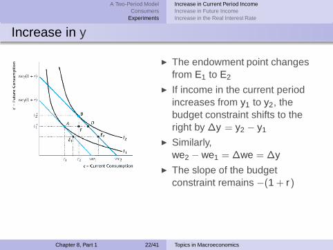
◮ The endowment point changesfrom E1 to E2

◮ If income in the current periodincreases from y1 to y2, thebudget constraint shifts to theright by ∆y = y2 − y1

◮ Similarly,we2 − we1 = ∆we = ∆y

◮ The slope of the budgetconstraint remains −(1 + r)



Experiments


Increase in y

◮ Since current and futureconsumption are normal goods,both will increase

◮ Notice that the increase incurrent consumption (AF ) issmaller than the increase incurrent income (AD)

◮ It follows that ∆s = ∆y − ∆c > 0◮ Conclusion: an increase in y

◮ Increases c and c′

◮ Increases s



Experiments


Measuring Consumption Smoothing

◮ The prediction of the model is that consumers want tospread an increase in income by consuming more inseveral periods, i.e. they smooth consumption over time

◮ Recall from Chapter 3 that consumption is less volatilethan income (85% as volatile)

◮ Furthermore, consumption is measured as purchases ofdurables plus non-durable goods, not the actualconsumption

◮ But durable (consumption) goods (e.g. a new car) aremore like an investment good

◮ It turns out that consumption (as measured bynon-durables only) is indeed much less volatile thanincome, which is consistent with consumption smoothing



Experiments


Consumption Smoothing in the Data



Experiments


Excess sensitivity of Consumption

◮ While consumption is less volatile than income in the data,it is still not smooth enough to be in line with this theory

◮ Two reasons are given for this excess sensitivity ofconsumption:

1. Imperfections in the credit marketOur theory assumes that consumers can freely borrow andlend at rate r to smooth consumption, which may not be agood assumption

2. Market prices will change if all consumers want to smoothconsumption simultaneously

We have not taken general equilibrium effects into accountyet: if all consumers want to lend, the interest rate willchange in a way that makes consumers want to consume!



Experiments


Increase in y ′

◮ If income tomorrow is expectedto increases from y ′

1 to y ′

2, thebudget constraint shifts up by∆y ′ = y ′

2 − y ′

1

◮ Lifetime wealth also increasesfrom we1 to we2

◮ The slope of the budgetconstraint remains −(1 + r)



Experiments


Increase in y ′

◮ Since current and futureconsumption are normal goods,both will increase

◮ Notice that current consumptionincreases but current income isunchanged

◮ It follows that ∆s = −∆c < 0◮ Conclusion: an increase in y ′

◮ Increases c and c′

◮ Decreases s



Experiments


Temporary vs Permanent Changes in Income

◮ The Permanent Income Hypothesis (PIH) stipulates thatthe main determinant of consumption is permanentincome, which is closely related to lifetime wealth

◮ Since a temporary change in income has a small impact onpermanent income, it has a small impact on consumption

◮ Since permanent change in income has a large impact onpermanent income, it has a large impact on consumption

◮ In our model, consumption increases more if incomeincreases in both periods than if income increases in onlyone period — the impact on savings is much smaller



Experiments


Increase in r

◮ Decreases the horizontalintercept (present valuedisposable income is lower)

we2 = y − t + y ′−t′

1+r2

◮ Increases the vertical intercept◮ The value of first period income

in the second period is higherthan before (1 + r2)(y − t)

◮ The value of second periodincome in the second periodhas not changed (y ′ − t ′)

◮ Rotates the budget line aroundthe endowment point, with asteeper slope of −(1 + r2)



Experiments


Increase in r for a Lender: Substitution Effect

◮ Under r1, the consumer choosespoint A:c1 < y − t so s > 0

◮ Under r2, the consumer choosespoint B

◮ The substitution effect is themovement from A to D

◮ Since the relative price of futureconsumption is lower:

◮ c decreases◮ c′ increases◮ s increases



Experiments


Increase in r for a Lender: Income Effect

◮ The income effect is themovement from D to B

◮ Since the consumer is richer andgoods are normal:

◮ c increases◮ c′ increases◮ s decreases



Experiments


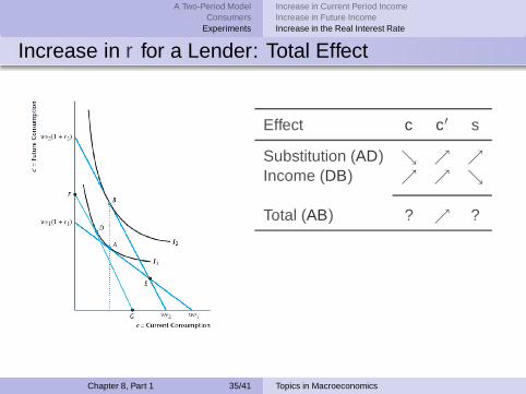
Increase in r for a Lender: Total Effect

Effect c c′ s

Substitution (AD) ց ր ր

Income (DB) ր ր ց

Total (AB) ? ր ?



Experiments


Increase in r for a Borrower: Substitution Effect

◮ Under r1, the consumer choosespoint A:c1 > y − t so s < 0

◮ Under r2, the consumer choosespoint B

◮ The substitution effect is themovement from A to D

◮ As before, since the relative priceof future consumption is lower:

◮ c decreases◮ c′ increases◮ s increases



Experiments


Increase in r for a Borrower: Income Effect

◮ The income effect is themovement from D to B

◮ Since the consumer is poorerand goods are normal:

◮ c decreases◮ c′ decreases◮ s increases



Experiments


Increase in r for a Borrower: Total Effect

Effect c c′ s

Substitution (AD) ց ր ր

Income (DB) ց ց ր

Total (AB) ց ? ր



Experiments


Increase in r : Aggregate Effect

For Lenders

Effect c c′ s

Substitution ց ր ր

Income ր ր ց

Total ? ր ?

For Borrowers

Effect c c′ s

Substitution ց ր ր

Income ց ց ր

Total ց ? ր

The aggregate impact depends on◮ The relative size of income and substitution effects◮ The number of borrowers and lenders



Experiments


The Demand for Current Consumption (cd)

◮ An increase in current incomeincreases current consumptionless than one for one

◮ So the slope of cd is less thanone

◮ The slope of cd is called themarginal propensity toconsume (MPC)

◮ We know that the MPC < 1◮ The MPC may vary with the

income level



Experiments


Factors that Increase the Demand for CurrentConsumption

The cd curve will shift up if◮ The interest rate falls and the

intertemporal substitution effectdominates the income effect

◮ The present value of taxesdecreases

◮ Future income increases


a two-period model: the consumption–savings · pdf file · 2010-03-12a...

Documents