optimal conjunctive use of groundwater and recycled wastewater
TRANSCRIPT
Optimal Conjunctive Use of Groundwater and Recycled
Wastewater
James Roumasset*
Department of Economics University of Hawai‘i at Mānoa
& University of Hawai‘i Economic Research Organization
Christopher Wada† University of Hawai‘i Economic Research Organization
Working Paper No. 10-13
August 11, 2010
Abstract: Inasmuch as water demand is multifaceted, infrastructure planning should be part of a general specification of efficient quantities and qualities of water deliveries over time. Accordingly, we develop a two-sector dynamic optimization model to solve for the optimal trajectories of groundwater extraction and water recycling. For the case of spatially increasing costs, recycled water serves as an intermediate resource in transition to the desalination steady state. For constant unit recycling cost, recycled wastewater eventually supplies non-potable users as a sector-specific backstop, while desalination supplements household groundwater in the steady state. In both cases, recycling water increases welfare by shifting demand away from the aquifer, thus delaying implementation of costly desalination. Implementation of the model provides guidance on the appropriate timing and size of backstop and recycling infrastructure as well as water deliveries from the various sources to the water-demand sectors. Keywords: Renewable resources, dynamic optimization, groundwater allocation, wastewater reuse, recycling, reclamation, water quality JEL codes: Q25, Q28, C6
* Professor, Department of Economics, University of Hawai‘i, Mānoa, and Research Fellow for the University of Hawai‘i Economic Research Organization, Saunders 542, 2424 Maile Way, Honolulu, HI 96822 USA. E-mail: [email protected] † Postdoctoral Research Economist, University of Hawai‘i Economic Research Organization. E-mail: [email protected]

1 Introduction
Water scarcity has long been an important issue in many regions around the world,
and the threat of climate change has recently brought it even further to the forefront of
policy discussions. The United Nations (2006) recommends a multidisciplinary approach
to managing water scarcity, inasmuch as “water scarcity affects all social and economic
sectors and threatens the sustainability of the natural resources base.” While demand for
water continues to grow, a plethora of both demand- and supply-side management
strategies are being considered, including but not limited to expansion of existing
reservoirs or creation of new ones, watershed conservation, more efficient conjunctive
use of ground and surface water, new pricing structures, voluntary or mandatory quantity
restrictions, and implementation of wastewater recycling and desalination.
The recycling of urban wastewater refers to the process of using treated
wastewater for various purposes, including artificial recharge of groundwater basins,
irrigation for landscaping or agriculture, and industrial processes that do not require
potable water such as cooling. Wastewater can be treated to varying degrees and the
resulting level of quality ultimately constrains the recycled water to particular end-uses.
Table 1. Adopted from Abu-Zeid (1998)
Treatment: Preliminary Primary Secondary Tertiary What gets removed:
Large solids Settleable solids by sedimentation
Organic matter Nitrogen, phosphorus, detergents, softeners, and heavy metals
Agricultural uses:
Non-consumed crops (e.g. wood trees)
Non-consumed crops (e.g. cotton) or non-leafy crops (e.g. orchards)
Animal food crops, food crops with inedible skins, and heat-processed fruits
Raw consumed plants

In many regions, recycled water is used mainly for agriculture (Table 1), but the
same potential cost advantage exists for primarily urban economies, in which industry is
a larger sector than agriculture. Al-Zubari (1998) estimates that for Bahrain, secondary
treatment of wastewater costs $0.164/m3 ($0.62/tg), tertiary treatment costs $0.317/m3
($1.20/tg) and desalinated water costs $0.794/m3 ($3.01/tg). If environmental regulations
require at minimum secondary treatment for disposal, the additional unit cost (not
inclusive of infrastructure expansion costs) of tertiary treatment is relatively small. Thus
the marginal cost of a unit of recycled water is likely lower than that of higher quality
sources (e.g. groundwater or desalination).
Analyses in the engineering literature have begun to incorporate recycling as an
option in large portfolios of water management strategies, but most of these studies do
not optimize water use in a truly economic sense. The CALVIN (California value
integrated network) model, for example, allocates water statewide within physical,
environmental, and selected policy constraints, but its objective is to “maximize the year
2020 net economic benefits of water operations and allocations to agricultural and urban
water users” (Jenkins et al., 2001; Draper et al., 2003; Jenkins et al., 2004), not the
present value of the stream of net benefits accruing now and in the future as is generally
the practice in resource economics. Wilkinson and Groves (2006) also develop a large-
scale model whose purpose is to consider the “impact of alternative levels of groundwater
conjunctive use and municipal wastewater reuse on long-term supply and demand
balance in the region.” The model allows a planner to consider the effects of various
programs through specification of scenario-specific parameters, i.e. the model does not

solve for the optimal economic allocation. Thus, fundamental analytical work on the
economics of recycled water remains to be done.
In the absence of recycled water, demand growth necessitates the eventual
implementation of a costly but abundant backstop resource such as desalination, even if
existing water resources are allocated optimally over time to maximize net social benefits
(Krulce et al., 1997). The concept of a backstop technology is already established in the
groundwater economics literature, even for the case of multiple demand sectors
(Koundouri and Christou, 2006). However, little attention has been paid to recycled water
and its potential role as an intermediate or sector-specific backstop. Inasmuch as different
demand sectors require different qualities of water (e.g. potable vs. non-potable),
different resources can serve as backstops for each respective sector.
In developing and solving a dynamic groundwater-economics model to optimize
water extraction for two demand sectors, we establish the concepts of an intermediate and
a sector-specific backstop. The general model allows for increasing unit recycling costs
to implicitly incorporate infrastructure expansion costs for spatially differentiated users.
The order of resource extraction for each demand sector optimally follows a least-
marginal-opportunity-cost-first rule where the marginal opportunity cost includes
extraction, distribution, and endogenous marginal user cost. Recycled water serves as an
intermediate resource for non-potable water users in transition to the desalination steady
state. We also consider constant unit recycling costs as a special case of the model. In
some situations, it may make sense to amortize capital costs to determine a single
constant unit cost of recycling. For constant unit recycling cost, recycled wastewater
eventually supplies non-potable users as a sector-specific backstop, while desalination

supplements groundwater in the household sector steady state. In both cases, recycling
water increases welfare by shifting demand away from the aquifer, thus delaying
implementation of costly desalination.
2 The model
Groundwater is modeled as a renewable and replaceable resource. Coastal
aquifers, often characterized by a “Ghyben-Herzberg” lens (Mink, 1980) of freshwater
sitting on an underlying layer of seawater, are “renewable” in that net recharge to the
aquifer varies with the groundwater stock. The upper surface of the freshwater lens sits
above sea level due to the difference in density between the freshwater and displaced
saltwater. The head level (h), or the distance between the top of the lens and mean sea
level is a measure of the aquifer stock. Although the stored volume is technically a
function of rock porosity, lens geometry and other hydrologic parameters, the head-
volume relationship can be approximated as linear (e.g. Krulce et al. 1997; Pitafi and
Roumasset, 2009). Thus, as the stock declines, the head level falls proportionately, and
groundwater extraction becomes more costly, inasmuch as water must be lifted a longer
distance to the surface. Unit groundwater extraction cost is a non-negative, decreasing,
convex function of head: , 0)( ≥tG hc 0)( <′ tG hc , and 0)( ≥′′ tG hc .
Leakage from a coastal aquifer is also a function of the head level. In many
coastal aquifer systems, low permeability sediment deposits bound the freshwater lens
along the coast, but pressure from the lens causes some freshwater to leak or discharge
into the ocean as springflow and submarine groundwater discharge. As the head level
declines, leakage decreases both because of the smaller surface area along the ocean
boundary and because of the decrease in pressure due to the shrinking of the lens. Thus,

leakage is a positive, increasing, convex function of head: , , and
. Infiltration to the aquifer from precipitation and adjacent water bodies is fixed
at a constant rate (I).
0)( ≥thL 0)( >′ thL
0)( ≥′′ thL
Inasmuch as water demand is multifaceted, from a long-term perspective,
infrastructure choice should match the varying characteristics of water required for
different end-users in terms of quantity and quality. The cost of distributing ground or
surface water to users located far from the reservoir or groundwater facility can be non-
trivial, but additional infrastructure is only required if new users are beyond the existing
network of pipes for potable water conveyance. Non-potable recycled water, on the other
hand, requires its own pipes and meters, regardless of the location. Thus, if recycled
water users are highly spatially differentiated, infrastructure and distribution costs can
quickly escalate with distance from the treatment facility, making recycled water a less
cost-effective and hence less desirable resource for distant users.
Properly characterizing the cost of recycled water requires incorporating
infrastructure investment into the optimization model. Lumpy investment could be
introduced explicitly, but the same general insights can be obtained by assuming that the
unit cost of recycling is an increasing and convex function of recycled water, i.e.
, , and . Implicitly, treatment facilities are first
constructed near agricultural or industrial centers, i.e. where the concentration of
potential recycled water users is highest. The distribution network endogenously expands
over time, until eventually it becomes beneficial to build additional treatment plants or to
supplement with an alternative resource. For a continuum of non-potable water users,
cost increases convexly with units of recycled water because more energy is required to
0)( >RtR qc 0)( >′ R
tR qc 0)( ≥′′ RtR qc

pump water a greater distance, additional treatment facilities may need to be constructed,
and costly pipes and meters must be installed for each additional consumer.
Generally, with multiple end-uses or demands and varying qualities of water,
users are naturally classified into categories by quality requirements. In some cases,
benefits for certain uses may vary by input water quality so that optimality would not
always necessitate using the minimum allowable quality for each use. To make the model
more tractable and transparent, however, we aggregate non-potable uses into a single
demand category (agriculture), and there is no additional benefit to using higher quality
water than necessary. Groundwater is the primary source of high quality (potable) water.
No surface water is available, but lower quality (non-potable) water can be obtained from
wastewater recycling. In addition, desalinated seawater serves as a high quality backstop
resource. High quality water can be utilized for both potable and non-potable uses, but
recycled water cannot supply the residential/household demand sector.
The production of recycled water is constrained by the quantity of wastewater
input and the efficiency of the treatment process. Not all ground or desalinated water
used by households enters the sewage system. On average, some proportion, , is
utilized for watering lawns and other outdoor purposes. Of the water that does ultimately
enter the sewage treatment facility, a fraction,
)1,0(1 ∈b
)1,0(2 ∈b
)BHt
, is lost during the treatment
process (e.g. as sludge). Consequently, the maximum feasible total production of
recycled water in a given period is , where ( GHt qq +β )1)(1( 21 bb −−≡β is the
proportion of groundwater ( ) and desalinated water ( ) used by the household
sector that can be effectively recycled.
GHtq BH
tq

The water manager chooses the rates of groundwater extraction for the household
sector and the agricultural sector , the rates of desalination for household
and agricultural use , and the rate of wastewater recycling to
maximize the present value of net social benefit, measured as gross consumer surplus less
total costs:
)( GHtq )( GA
tq
)( BHtq )( BA
tq )( RAtq
(1) dt
qcqcqqhcqq
dxtxDdxtxDeMax
RAtR
RAtB
BAt
BHttG
GAt
GHt
qqq
A
Ht
qqqqq
BAt
RAt
GAt
BHt
GHt
BAt
RAt
GAt
BHt
GHt
∫ ∫∫∞++−
+−
−
⎪⎭
⎪⎬
⎫
⎪⎩
⎪⎨
⎧
−+−+
−+
00
1
0
1
,,,,
)()()()(
),(),(δ
subject to , )()( GAt
GHttt qqhLIh +−−=&γ
, 0)( ≥−+ RAt
BHt
GHt qqqβ
where is the inverse demand function for sector i=H,A, )(1 •−iD δ is the positive discount
rate, c is the unit cost of desalinating seawater, and B γ is a head-to-volume conversion
factor. To incorporate the recycling capacity constraint, we augment the CV Hamiltonian
into a Lagrangian function as follows:
(2) ⎪⎩
⎪⎨
⎧
−+++−−+−
+−+−+=Λ ∫∫
++−
+−
],)([)]()([)(
)()()(),(),(0
1
0
1
RAt
BHt
GHtt
GAt
GHttt
RAtR
RAt
BBAt
BHttG
GAt
GHt
qqq
A
H
qqqqqhLRqcq
cqqhcqqdxtxDdxtxDBAt
RAt
GAt
BHt
GHt
βμλ
and the Maximum Principle requires that the following conditions hold:
(3) 0)(),(1 ≤+−−+=∂Λ∂ −
tttGBHt
GHtHGH
t
hctqqDq
βμλ if < then 0=GHtq
(4) 0),(1 ≤+−+=∂Λ∂ −
tBBHt
GHtHBH
t
ctqqDq
βμ if < then 0= BHtq
(5) 0)(),(1 ≤−−++=∂Λ∂ −
ttGBAt
RAt
GAtAGA
t
hctqqqDq
λ if < then 0=GAtq

(6) 0)(),(1 ≤−′−−++=∂Λ∂ −
tRRAt
RAtR
BAt
RAt
GAtARA
t
cqqctqqqDq
μ if < then 0=RAtq
(7) 0),(1 ≤−++=∂Λ∂ −
BBAt
RAt
GAtABA
t
ctqqqDq
if < then 0= BAtq
(8) )()()( tttGGAt
GHt
ttt hLhcqq
h′+′+=
∂Λ∂
−=− λδλλ& .
Along the optimal trajectory, the marginal benefit must be equated to the marginal
cost of each water resource used in each demand sector. Given our assumption that
recycled water is perfectly substitutable for groundwater in the agricultural sector, the
marginal benefit, , is the same, regardless of the source. Similarly, since
groundwater and desalinated water are assumed to be perfect substitutes,
represents the marginal benefit of water in the household sector. The full marginal cost or
marginal opportunity cost (MOC) of a resource includes not only extraction or treatment
cost, but also marginal user cost. The MOC of groundwater and desalinated water for use
in the household sector is and respectively.
Similarly, the MOC of groundwater, desalinated water, and recycled water for use in the
agricultural sector is , , and
respectively. We define the efficiency price for each sector as that which induces the
optimal trajectory of water consumption, i.e. the marginal benefit along the optimal paths.
For and , conditions (3)-(7) can be simplified to
)(1 •−AD
GAtπ
Atp
)(1 •−HD
BBAt c≡π
tttGGHt hc βμλπ −+≡ )(
ttG hc λ+≡ )( RRAt qcπ ≡ (
)(1 •≡ −AD
tBBHt c βμπ −≡
tRRAt cq μ+′+RA
t )
)(1 •≡ −H
Ht Dp
(9) },min{ BHt
GHt
Htp ππ=
(10) },,min{ BAt
RAt
GAt
Atp πππ=

The price of water for household use is determined by the lower of either the
MOC of groundwater or the MOC of desalination. Similarly, the price of water for
agricultural use is the minimum of the MOC of groundwater, recycled wastewater, and
desalinated seawater. When the recycling capacity constraint is not binding, the MOCs of
groundwater are equal in both sectors, as are the MOCs of desalinated water. When the
constraint is binding, however, tμ is the shadow value of an additional unit of recycled
water. In optimality conditions (3) and (4), tβμ is subtracted from the costs because using
an additional unit of ground or desalinated water relaxes the recycling constraint and adds
to the PV by exactly that amount. On the other hand, tμ is added to the costs for
condition (6) because more recycled water would be used in the absence of the binding
constraint. Although the MOC of desalination is constant in both sectors aside from the
recycling constraint, the MOCs of groundwater and recycled water are variable. In
particular, unit groundwater extraction cost rises as the head level declines, and marginal
user cost rises as the resource becomes scarcer. For the reasons previously discusses, unit
recycling cost varies with the quantity recycled.
2.1 Steady state
Inasmuch as demand growth ensures desalination in the steady state for both
sectors, as per condition (4). That the steady state requires means
groundwater extraction for the household sector must be positive, and combining
condition (3) with the previous result yields
TBHT cp βμ−= 0=h&
)( TGBT hcc −=λ . Taking and p0=λ& lugging

Tλ into condition (8) results in a single equation that can be solved for the unique1 st
state aquifer head level ( ∗Th ):
eady
(11) )(
)]()[( Th+δ
)(T
TGTGB hL
hLIchcc′−′
−=
.
2.2 Order of resource use
In this section, we consider three possible scenarios: (a) the unit cost of
desalination exceeds the unit cost of recycled water, which exceeds the initial MOC of
groundwater; (b) the unit cost of desalination is greater than the initial MOC of
groundwater, which is greater than the unit cost of recycled water; and (c) the initial
MOC of groundwater is the highest, followed by the unit cost of desalination and then the
unit cost of recycled water.
If the aquifer starts in a relatively pristine state, then the initial MOC of
groundwater might lie below the cost of the first unit of recycled water. In that case,
groundwater optimally supplies both demand sectors in the initial stage of extraction. The
MOC of groundwater rises rapidly over time until it reaches the cost of the first unit of
recycled water. Groundwater continues to supply both sectors, but as the MOC of
groundwater continues to rise, more of the water consumed by the agricultural sector is
supplied by recycling, i.e. the network of recycling infrastructure is endogenously
expanded as more users optimally switch to the lower quality source. In the steady state,
all water resources are used; recycled water is used for the agricultural sector, and
desalinated water and groundwater are used for both sectors.
If instead the unit desalination cost exceeds the initial MOC of groundwater, and
the initial MOC of groundwater exceeds the unit cost of recycled water for the first unit,
1 See the appendix for a proof of this result.

then groundwater is extracted exclusively for the household sector and at least some
water is recycled for the agricultural sector from the outset. Recycled water is used
exclusively for the agricultural sector if the MOC of recycled water at the demand curve
is below the MOC of groundwater (and the quantity constraint is not binding). If not,
recycled water is used until the MOC of the last unit is just equal to the MOC of
groundwater, and groundwater is extracted to satisfy the remainder of the quantity
demanded. As the MOC of groundwater rises, more of the agricultural sector’s demand is
met by recycled water. In the steady state, all water resources are used.
A third possibility is that the aquifer is severely depleted such that the MOC of
groundwater starts above the unit cost of desalination. Recycled water is used exclusively
by the agricultural sector, unless the quantity constraint is binding or the MOC exceeds
the unit cost of desalination at the demand curve, in which case recycling is
supplemented by desalination. Desalination is used exclusively by the household sector.
The aquifer is allowed to build until the MOC of groundwater falls to the unit cost of the
backstop, at which point groundwater and desalination are used simultaneously. In the
mean time, the number of recycled users steadily increases until the steady state. Further
demand growth in the agricultural sector necessitates eventual supplementation by
desalination. The stages of resource use for each scenario are summarized in table 2.
Table 2. Stages of Resource Use
Scenario\Stage 1 2 3 a GW for H
GW for A GW for H GW + RW for A
GW + DW for H GW + RW + DW for A
b GW for H RW (+ GW) for A
GW + DW for H GW + RW + DW for A
c DW for H RW (+ DW) for A
GW + DW for H GW + RW + DW for A
Note: GW = groundwater, DW = desalinated water, RW = recycled water; H = household, A = agriculture.

Figure 1. Network of recycled water users expands over time in the agricultural
sector. When water recycling is incorporated into an optimal groundwater management
plan, the boundary of recycled water users shifts out over time as the scarcity value of
groundwater increases (figure 1).2 Although the approach path may be non-monotonic,
the aquifer head level is eventually drawn down toward its steady state level (SW
quadrant of figure 1). As the aquifer is depleted, groundwater becomes scarcer, and its
MOC shifts upward (NW quadrant). Given the choice between groundwater and recycled
water for the agricultural sector, the source with the lowest MOC is used first. For the
head level h1, and the corresponding groundwater MOC1, the optimal quantity of recycled
water is q1 (NE quadrant). Up until that quantity, the unit cost of recycled water is lower
than the MOC of groundwater, i.e. CR(qR) < MOC1. The remainder of the quantity 2 To maintain graphical clarity, the demand curve is depicted as constant over time. Growing demand does not change the qualitative result that the network of recycled users expands over time.
MOC0
CR(qR) MOCGW
$
MB
MOC1
MOC2
q2q1 h2 qE h1 h0 h
t

demanded is met by groundwater at unit cost MOC1. In later periods, the MOC of
groundwater is even higher, which means more recycled water is used, and the boundary
of recycled water users expands over time (SE quadrant). Eventually, the system reaches
a steady state, at which time expansion ceases and recycling infrastructure is sustained,
while the remainder of consumption is met by desalination.
Another way to depict the stages of optimal resource use is to compare directly
the time path of each resource’s MOC for each demand sector. We again illustrate the
optimal program for scenario a because it is the most complex of the three. The
hypothetical time paths for the other two scenarios can be constructed in a similar
manner. For and , groundwater is used initially in both
sectors (figure 2a and 2b). As groundwater scarcity rises, it eventually becomes optimal
to use recycled water in the agricultural sector, i.e. . Meanwhile in the
household sector, the scarcity value of groundwater “kinks” slightly because recycling in
the agricultural sector lowers groundwater extraction costs by conserving on freshwater.
Eventually, the MOC of groundwater and that of recycled water both rise to the MOC of
desalination, and the system reaches a steady state. The qualitative welfare implications
of the optimal recycling program are revealed when comparing the MOC trajectories to
those that would obtain under groundwater optimization alone (figure 2c and 2d).
Without recycling, groundwater is used by both sectors until the steady state.
Consequently, extraction costs rise more rapidly, as does groundwater scarcity, meaning
desalination must be implemented earlier in both sectors. Clearly, implementation of
optimal wastewater recycling increases the present value net benefit to society, inasmuch
BARAGA000 πππ << BHGH
00 ππ <
RAGA0ππτ =

as the lower extraction path allows for an extended period of drawdown before
implementation of costly desalination in the steady state.
BAπ
GAπ GHπ
BHπ
TH
TH
TA
TA
GHπ
BHπ BAπ
RAπ
(b) (a)
GAπ
RA0π
τ
(d) (c)
Figure 2. Hypothetical time paths of MOCs: (a) Agricultural sector with recycling, (b) Household sector with recycling, (c) Agricultural sector without recycling, (d)
Household sector without recycling.
2.3 Proposed solution method
In the previous section, we discuss the ordering of water resource use as if we
already know the optimized MOC paths for each resource within each demand sector.
However, solving the problem in practice involves consideration of multiple trial MOC
paths, only one of which maximizes PV. It is useful to think of the problem in discrete
time for the purpose of computation. If the quantity constraint on recycling is never
binding, then the solution method based on the discrete-time analogues of equations (3)-

(10) is fairly straightforward. A trial value is assumed for the initial shadow price of
groundwater, and condition (8) allows one to determine the shadow price in the following
period. The efficiency price for each sector can then be ascertained from equations (9)
and (10) for the current period. The price reveals the current-period rates of extraction,
recycling, or desalination. The equation of motion for the aquifer generates the head level
for the next period, and the whole process can be repeated, starting with the next period
shadow price and head level. Eventually, one of the terminal conditions is reached; either
the head level declines to or one of the efficiency prices rises to the unit backstop cost.
If the conditions do not coincide, i.e. one is inconsistent, the trial value for the initial
shadow price of groundwater is revealed as incorrect. The guess must be adjusted and the
process repeated until all of the initial and terminal conditions are satisfied for the head
level and the efficiency prices in each sector, so that the PV functional is maximized.
∗Th
If instead the recycling quantity constraint is binding for a finite period, then the
computational method should be adjusted. Starting again with condition (8), a trial value
for the shadow price of groundwater allows one to solve for the shadow price in the
following period. Inasmuch as condition (5) does not depend on the Lagrangian
multiplier, one can then determine the efficiency price in the agricultural sector. The
price determines the quantity of recycled water, and the quantity of groundwater for the
agricultural sector is just the residual of the total quantity demanded at that price. If
groundwater is being used in the agricultural sector, it must also be used in the household
sector. Condition (3) can be used to solve for the quantity of groundwater in the
household sector for 0=tμ . One can then test the quantity constraint, i.e. check that
. If the constraint is not binding, then the aquifer equation of motion RAt
BHt
GHt qqq >+ )(β

generates the head level for the next period. If it is binding, then .
Since that does not change the efficiency price in the agricultural sector, condition (6)
allows one to determine the value of the Lagrangian multiplier, and the quantity of
groundwater used in agriculture is still the residual of the total quantity demanded at that
price. Finally, given the value for
)( BHt
GHt
RAt qqq += β
0>tμ , condition (4) yields optimal rate of
groundwater extraction in the household sector.
2.4 A special case: constant unit recycling cost
In the case that lumpy infrastructure investment timing is not as crucial (e.g. when
the non-household sector is relatively small and stable, and a single treatment facility’s
capacity would be sufficient) one could use standard amortization methods to
approximate a constant unit cost of recycling ( ). Since recycled water is of less than
potable quality, it is a reasonable assumption that the unit cost of wastewater recycling is
less than the unit cost of desalinating seawater, i.e.
Rc
BR cc < . Recycled water serves as a
sector-specific backstop for the agricultural sector. Groundwater is used in every period
for household consumption, but recycled water eventually serves the entire agricultural
sector in the steady state. Analogous to the general case with rising unit recycling cost,
stages of resource use leading to the steady state are determined by the ordering of the
three MOCs in each of the demand sectors. Table 3 summarizes the stages of resource
use for the same three scenarios discussed in the general cost case.

Table 3. Stages of Resource Use (Constant Unit Recycling Cost)
Scenario\Stage 1 2 3 a GW for H
GW for A GW for H RW for A
GW + DW for H RW for A
b GW for H RW for A
GW + DW for H RW for A
c DW for H RW for A
GW + DW for H RW for A
Note: GW = groundwater, DW = desalinated water, RW = recycled water; H = household, A = agriculture.
3 Conclusion
Efficient management of water resources requires optimization over multiple
margins, including the development of supplementary resources. Wastewater recycling
can delay the costly implementation of desalination but a question arises regarding
composition and timing of the requisite investments. Inasmuch as different demand
sectors require different qualities of water, it is natural to think of recycled water as an
intermediate resource for those users with low water quality requirements. When unit
recycling cost is constant, recycled water serves as a sector-specific backstop.
Implementation of the model provides guidance on the appropriate timing and size of
backstop and recycling infrastructure.
The necessary conditions derived from the optimal control problem accord with a
least-marginal-opportunity-cost-first extraction rule, where the marginal opportunity cost
of a particular resource is comprised of its extraction cost and endogenous marginal user
cost. Inasmuch as the marginal user cost of groundwater is stock-dependent and thus
variable over time and the marginal cost of recycled water is increasing in quantity
produced, various stages of extraction are possible, depending on initial values and other
parameters in the actual application. For example, groundwater may be used exclusively
in all sectors for a finite period of time, or it may be that recycled water or desalinated
water optimally supplements groundwater in any given period. Although recycled water
can never serve as a true backstop for the agricultural sector if demand is growing, it
eases the transition of usage from groundwater to desalinated water. More specifically, it
increases the present value to society by allowing an extended period of drawdown
before implementation of costly desalination.
Water quality is an aspect of the model that should be expanded on in future
research. The current model only differentiates between potable and non-potable water,
but in reality, there exists many levels of treated water for non-potable uses. While the
lowest quality recycled water is acceptable for uses such as industrial cooling, water used
for human crops generally requires at least secondary treatment. It remains to be seen
whether introducing more finely differentiated categories of end-uses as well as multiple
qualities would change the qualitative results presented here.
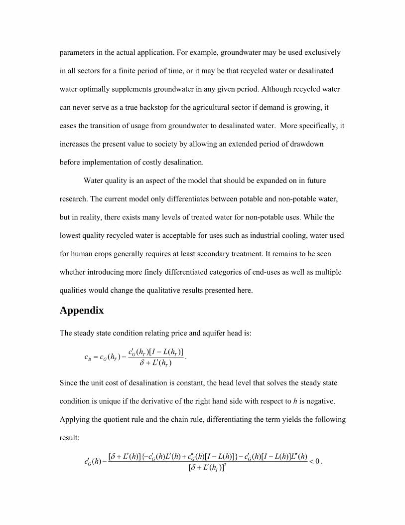
Appendix
The steady state condition relating price and aquifer head is:
)()]()[()(
T
TTGTGB hL
hLIhchcc′+−′
−=δ
.
Since the unit cost of desalination is constant, the head level that solves the steady state
condition is unique if the derivative of the right hand side with respect to h is negative.
Applying the quotient rule and the chain rule, differentiating the term yields the following
result:
0)]([
)()]()[()]}()[()()()]{([)( 2 <′+
′′−′−−′′+′′−′+−′
T
GGGG hL
hLhLIhchLIhchLhchLhcδ
δ .

That the term is negative follows from the assumed characteristics of the leakage and
extraction cost functions.
References
Abu-Zeid, K.M. (1998): “Recent trends and developments: reuse of wastewater in
agriculture,” Environmental Management and Health, 9(2): 79-89.
Al-Zubari, W.K. (1998): “Towards the establishment of a total water cycle management
and re-use program in the GCC countries,” Desalination, 120(2): 3-14.
Draper, A.J., Jenkins, M.W., Kirby, K.W., Lund, J.R. and R.E. Howitt (2003): Economic-
Engineering Optimization for California Water Management, Journal of Water
Resources Planning and Management, 129(3): 155-164.
Jenkins, M. W., et al. (2001): Improving California water management: Optimizing
value and flexibility, Center for Environmental and Water Resources Engineering,
Univ. of California, Davis, Davis, Calif. Available online at:
http://cee.engr.ucdavis.edu/faculty/lund/CALVIN.
Jenkins, M.W., Lund, J.R., Howitt, R.E., Draper, A.J., Msangi, S.M., Tanaka, S.K.,
Ritzema, R.S., and G.F. Marques (2004), Optimization of California’s Water
Supply System: Results and Insights, Journal of Water Resources Planning and
Management, 130(4): 271-280.
Koundouri, P. and C. Christou (2006): “Dynamic adaptation to resource scarcity and
backstop availability: theory and application to groundwater,” The Australian
Journal of Agricultural and Resoure Economics, 50, 227-245.
Krulce, D. L., J. A. Roumasset, and T. Wilson (1997): “Optimal management of a
Renewable and Replaceable Resource: The Case of Coastal Groundwater,”
American Journal of Agricultural Economics, 79, 1218-1228.
Mink, J. F. (1980): State of the Groundwater Resources of Southern Oahu. Honolulu:
Honolulu Board of Water Supply.
UN-Water, Coping with water scarcity: a strategic issue and priority for system-wide
action, 2006. www.unwater.org
Wilkinson, R. and D.G. Groves (2006), Rethinking Water Policy Opportunities in
Southern California: An Evaluation of Current Plans, Future Uncertainty, and
Local Resource Potential.