conjunctive use of surface and groundwater resources with

1

Conjunctive Use of Surface and Groundwater Resourceswith Emphasis on Water Quality

M. Karamouz1, M. Mohammad Rezapour Tabari2, R. Kerachian3 and B. Zahraie4

1Professor, School of Civil and Environmental Engineering, Amirkabir University (Tehran Polytechnic), Tehran, Iran. email: [email protected]. Student, School of Civil and Environmental Engineering, Amirkabir University (Tehran Polytechnic), Tehran, Iran. email: [email protected] Professor, Department of Civil Engineering, University of Tehran, Tehran, Iran. email: [email protected] Professor, Department of Civil Engineering, University of Tehran, Tehran, Iran. email: [email protected]

AbstractIn this paper, a methodology for conjunctive use of surface and groundwater resources with emphasis on water quality is developed using Genetic Algorithms (GAs) and the Artificial Neural Networks (ANNs). Water supply with acceptable quality, reduction of pumping costs, and controlling the groundwater table fluctuations are considered in the objective function of the model. In the proposed methodology, the results of a groundwater simulation model are used to train the ANNs based simulation model. This model is then linked to the GA based optimization model to develop the monthly conjunctive use operating policies. The proposed model is applied to the surface and groundwater allocation in the irrigation networks in the southern part of Tehran, the capital city of Iran.Tehran metropolitan area has annual domestic water consumption close to one billion cubic meters. The sewer system is mainly consisted of the traditional absorption wells. Some part of this sewage is drained into local rivers and drainage channels and partially contaminates the surface runoff and local flows. These polluted surface waters are used in conjunction with groundwater for irrigation purposes in the Southern part of the Tehran. The results of the proposed model show the significance of an integrated and systems approach to surface and groundwater resources allocation in the study area. For example, the cumulative groundwater table variations in each zone, which has experienced a total fluctuation of more than 20±meters in the last 20 years, is limited to 5± meters over the planning horizon

Keywords: Conjunctive Use, Artificial Neural Network, Genetic Algorithms, Groundwater Modeling, Water Quality

IntroductionMany investigators such as Maddock (1974); Onta et al. (1991); Yeh (1992); Fredericks et al. (1998); Loaiciga and Leipnik (2001); and Karamouz et al. (2004a, b) have used the systems approach and mathematical models in conjunctive surface and groundwater management. Most of the previous studies, presents the application of classical optimization models in conjunctive use planning. They also usually

Copyright ASCE 2005 EWRI 2005Downloaded 04 Nov 2008 to 129.116.232.152. Redistribution subject to ASCE license or copyright; see http://pubs.asce.org/copyright/

mailto:[email protected]



2

consider the simplified groundwater equations due to the computational burden of the problem. This paper deals with the development and application of an optimization and simulation models for analyzing regional water resources issues. In this paper, the PMWIN (Processing Modflow for Windows, developed by Chiang and Kinzelbach, 2001) model simulates the groundwater quantity and quality and then the groundwater response equations are explicitly developed by training a selected ANN. The proposed model is applied for conjunctive use of surface and groundwater resources considering the water quality in the southern part of Tehran. Considering the number of decision variables and the complexity of the system, a GA based optimization model is used to develop monthly operating policies.

Model FrameworkThe main objectives of the conjunctive use models are usually as follows:• Water supply to the agricultural demands• Improving the quality of allocated water• Minimizing the pumping costs• Controlling the groundwater table fluctuations

The model formulation for a 15-year planning horizon is as follows:

( ) ( )

( ) ( )

ncCZ

nLLZ

nHGHGZ

otherwisenDGQD

myniGQDif

Z

toSubject

ZMinimize

n

i y mimy

n

i y mimy

n

i y mimimimyimy

n

i y mimyimyimyimy

imyimyimy

iii

/)/)((

/)/)((

1215/)./.(

,1215//)(

12,...,1,15,...,1,,...,10

1

max

15

1

12

14

1

max

15

1

12

13

1

15

1

12

1max2

1

15

1

12

1

1

4

1

∑ ∑∑∑ ∑∑∑∑∑∑∑∑

∑

= = =

= = =

= = =

= = =

=

=

∆∆=

××=

××−−===+≤

=

:

α

12,...,1,15,...,1max ==∆≤∆ mLL yimy (1)

imyimyimy QRRD −= (2)

min,my

2

1iimy ERD ≥∑

=(3)

14

1ii =∑

=α (4)

12,...,1m,15,...,1y,n,...,1iRQ imyimy ===≤ (5)

)M~

,O~

,G~

(fL mymymyimy =∆ (6)


3

)c,M~

,O~

,G~

(fC mymymymyimy ′=∆ (7)

Where:

imyG : The volume of groundwater extracted in the agriculture zone i in month m of

year y ( daym /3 )

imyQ : The volume of surface water allocated to agriculture zone i in month m of

year y ( daym /3 )

imyC : The average concentration of the water quality indicator in the allocated water

to agriculture zone i in month m of year y ( Lmg / )

imyc : The average concentration of the water quality indicator in the return flow to

agriculture zone i in month m of year y ( daym /3 )

imyD : Agricultural water demand in zone i in month m of year y ( daym /3 )

imyL∆ : Variation of the groundwater table level in month m of year y in the

agriculture zone i (m) (draw down is considered to be negative).

maxL∆ : Maximum allowable cumulative groundwater table fluctuation (m)

maxC : Maximum allowable concentration of water quality variable in allocated

water ( L/mg )

imG : The volume of groundwater extracted in the agriculture zone i in month m

( day/m3 )

imyH : The groundwater table level in agriculture zone i in month m in year y

( )maximim HG × : Maximum value of ( )imim HG × in different years

imyR : Surface water flow rate in zone i in month m of year y

min,myE : Environment water demand in month m of year y

imyRD : Unused Surface water in zone i in month m of year y

1Z : Loss function of water allocation

2Z : Loss function of pumping cost

3Z : Loss function of groundwater table fluctuation

4Z : Loss function of the quality of allocated water

iα : Relative weight of the objective function i

m : Number of months in the planning horizonn : Number of agricultural zones in the study areay : Number of years in the planning horizon

The objective functions 1Z to 4Z should be normalized between 0 and 1. For this

purpose the relative weights iα can be assigned much easier based on the relative


4

importance of the objectives. Based on the constraint (1), the monthly variation of the water table level is limited to a maximum level. Equation (6), which is called the response function, presents the monthly groundwater table variations in each zone which is a function of the set of the volumes of the groundwater extracted in month

m of year y in the agricultural zones )G~

( my , the outflow at the boundaries, and the

groundwater discharge through springs and qanats in month m of year y ( myO~

),

recharge by direct precipitation, allocated surfacewater, and also recharge by absorption wells ( myM

~ ) This equation should be formulated using a comprehensive

groundwater simulation model.

GAs based Optimization ModelGAs use a random search technique that evolves the potential solution at a system using the genetic operators. Generation of the initial population, representation and encoding, selection, crossover, and mutation are the main steps in the GA based optimization models. The main characteristic of the Genetic Algorithms is presented by Gen and Chang (2000). In this study, the gene values are the monthly allocated ground and surface water to the agricultural zones. For example, when there are three agricultural zones and two surface water resources only for zones 1 and 2, the number of genes in a chromosome for a 15-year planning horizon is equal to 15*5*12=900, where 5 is the number of decision variables.

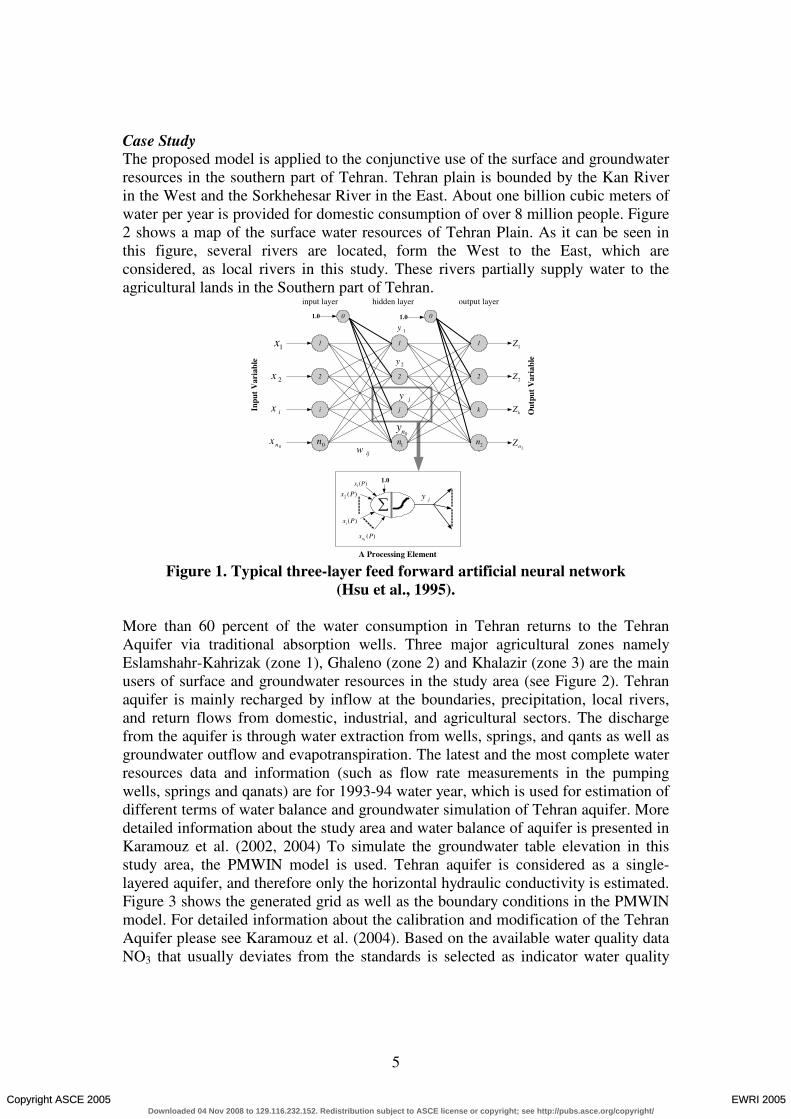
Groundwater Simulation using Artificial Neural NetworkThe groundwater table and quality variation equations are necessary for the proposed conjunctive use model (Equations 8 and 9). Considering the complexity of the system, the aquifer should be modeled using a comprehensive simulation model. As most of the groundwater quantity and quality simulation models (such as PMWIN) can not easily linked with optimization models, in this study a selected Artificial Neural Networks (ANNs) is trained using the results of the groundwater simulation.In this study, different ANNs have been tested and the multilayer feed forward networks have shown the best performance. Figure 1 shows the components of a typical three-layer feed forward artificial neural network. As it can be seen in this figure, each node j receives incoming signals from every node i in the previous

layer. Associated with each incoming signal ( )ix to node j , is a weight ( )jiw . The

effective incoming signal ( )js to node j is the weighted sum of all the incoming

signals:

∑=

= 0

0

n

iijij xws

Where 0x and 0jw are called the bias ( )0.10 =x and the bias weight, respectively.

The outgoing of node j is jy . More detailed information about the training of the

ANNs can be found in Hsu et al. (1995).


5

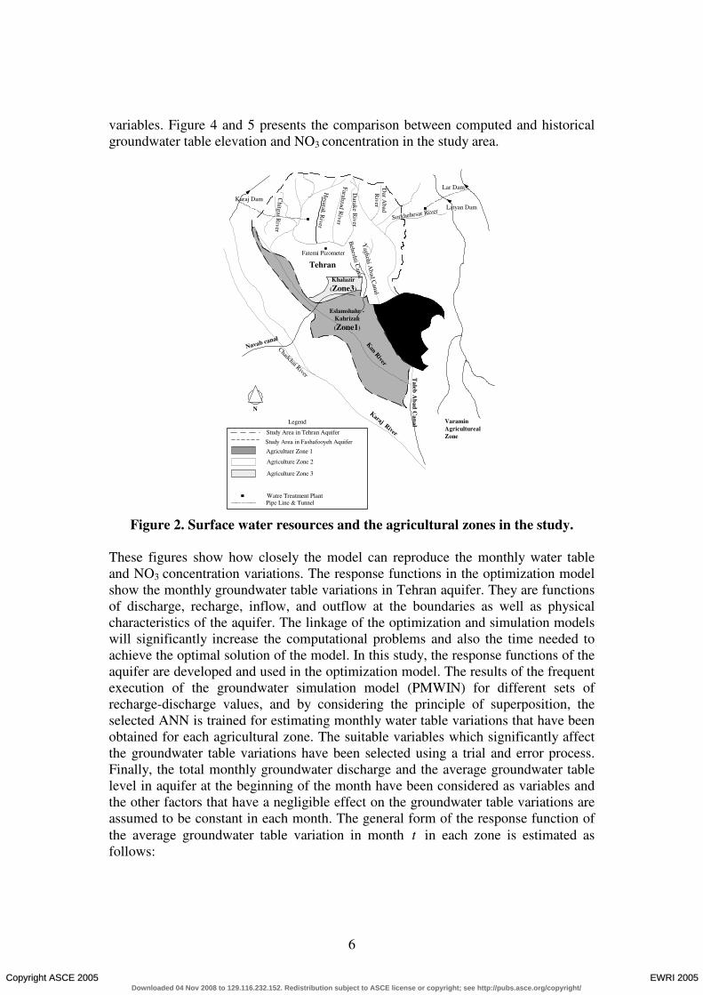
Case StudyThe proposed model is applied to the conjunctive use of the surface and groundwater resources in the southern part of Tehran. Tehran plain is bounded by the Kan River in the West and the Sorkhehesar River in the East. About one billion cubic meters of water per year is provided for domestic consumption of over 8 million people. Figure 2 shows a map of the surface water resources of Tehran Plain. As it can be seen in this figure, several rivers are located, form the West to the East, which are considered, as local rivers in this study. These rivers partially supply water to the agricultural lands in the Southern part of Tehran.

1

i

2

1

j

2

1

k

2

2n1n

1x

2x

ix

0nx

1y

2y

jy

1Z

2nZ

kZ

2Z

0 0

ijw

1.0 1.0

0n

input layer hidden layer output layer

Inpu

tV

aria

ble

Out

put

Var

iabl

e

0ny

∑1.0

)(0

Pxn

)(Pxi

)(2 Px

)(1 Px

jy

A Processing Element

Figure 1. Typical three-layer feed forward artificial neural network (Hsu et al., 1995).

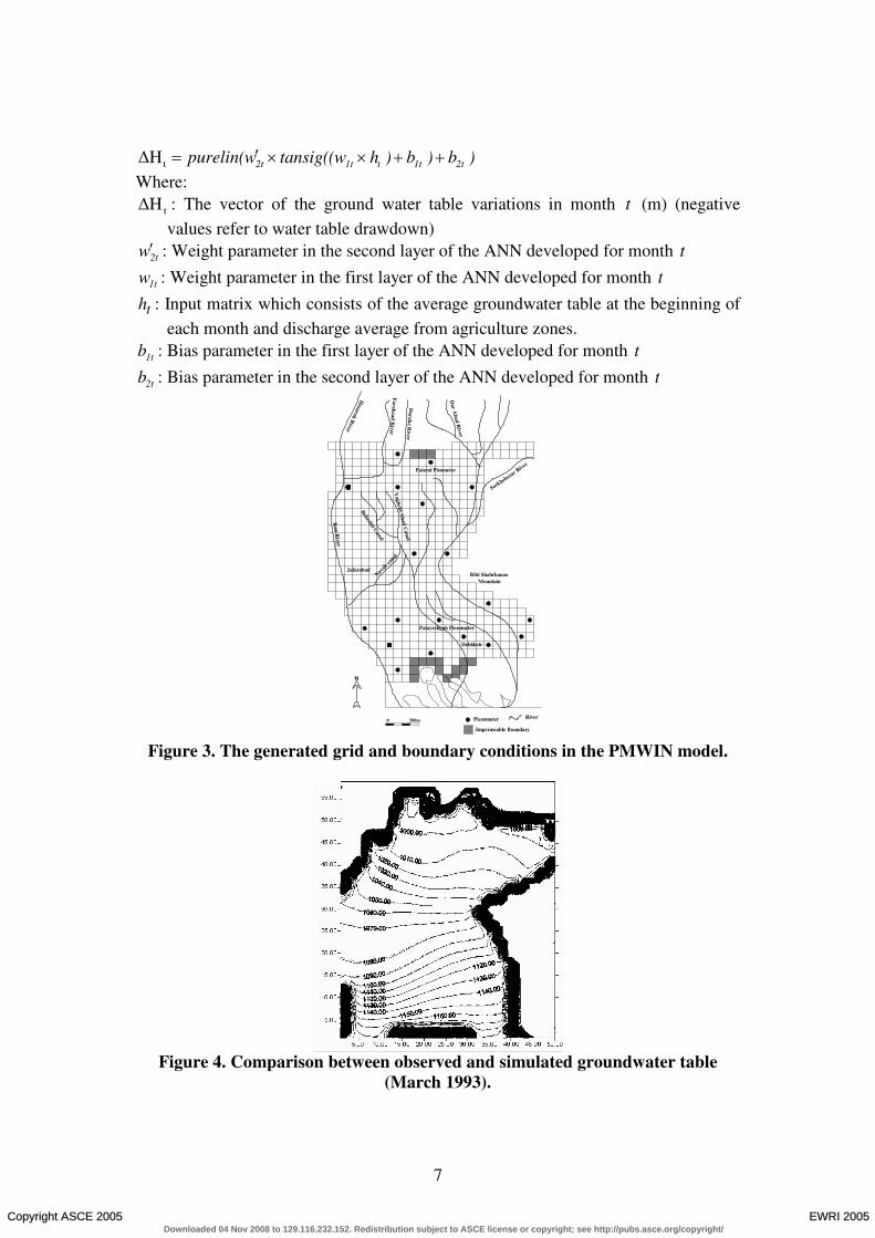
More than 60 percent of the water consumption in Tehran returns to the Tehran Aquifer via traditional absorption wells. Three major agricultural zones namely Eslamshahr-Kahrizak (zone 1), Ghaleno (zone 2) and Khalazir (zone 3) are the main users of surface and groundwater resources in the study area (see Figure 2). Tehran aquifer is mainly recharged by inflow at the boundaries, precipitation, local rivers, and return flows from domestic, industrial, and agricultural sectors. The discharge from the aquifer is through water extraction from wells, springs, and qants as well as groundwater outflow and evapotranspiration. The latest and the most complete water resources data and information (such as flow rate measurements in the pumping wells, springs and qanats) are for 1993-94 water year, which is used for estimation of different terms of water balance and groundwater simulation of Tehran aquifer. More detailed information about the study area and water balance of aquifer is presented in Karamouz et al. (2002, 2004) To simulate the groundwater table elevation in this study area, the PMWIN model is used. Tehran aquifer is considered as a single-layered aquifer, and therefore only the horizontal hydraulic conductivity is estimated.Figure 3 shows the generated grid as well as the boundary conditions in the PMWIN model. For detailed information about the calibration and modification of the Tehran Aquifer please see Karamouz et al. (2004). Based on the available water quality data NO3 that usually deviates from the standards is selected as indicator water quality


6

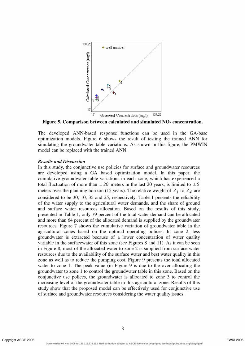
variables. Figure 4 and 5 presents the comparison between computed and historical groundwater table elevation and NO3 concentration in the study area.

Ghaleno

(Zone2)

Eslamshahr -Kahrizak

(Zone1)

Khalazir

(Zone3)T

aleb Abad C

anal

Kan River

Yaghchi A

bad Canal

Beheshti C

anal

Dar A

badR

iver

Darake R

iver

Farahzad River Sorkhehesar River

Hesarak R

iver

Chitgar R

iver

Fatemi Pizometer

Tehran

Navab canal

Karaj River

Chadchai River

Karaj DamLatyan Dam

Lar Dam

VaraminAgriculturealZone

N

Study Area in Tehran Aquifer

Study Area in Fashafooyeh Aquifer

Agricultuer Zone 1

Agriculture Zone 2

Agriculture Zone 3

Watre Treatment PlantPipe Line & Tunnel

Legend

Figure 2. Surface water resources and the agricultural zones in the study.

These figures show how closely the model can reproduce the monthly water table and NO3 concentration variations. The response functions in the optimization model show the monthly groundwater table variations in Tehran aquifer. They are functions of discharge, recharge, inflow, and outflow at the boundaries as well as physical characteristics of the aquifer. The linkage of the optimization and simulation models will significantly increase the computational problems and also the time needed to achieve the optimal solution of the model. In this study, the response functions of the aquifer are developed and used in the optimization model. The results of the frequent execution of the groundwater simulation model (PMWIN) for different sets ofrecharge-discharge values, and by considering the principle of superposition, the selected ANN is trained for estimating monthly water table variations that have been obtained for each agricultural zone. The suitable variables which significantly affect the groundwater table variations have been selected using a trial and error process. Finally, the total monthly groundwater discharge and the average groundwater table level in aquifer at the beginning of the month have been considered as variables and the other factors that have a negligible effect on the groundwater table variations are assumed to be constant in each month. The general form of the response function of the average groundwater table variation in month t in each zone is estimated as follows:


7

)b)b)htansig((wwpurelin( 2t1tt1t2t ++××′=t∆H

Where:

t∆H : The vector of the ground water table variations in month t (m) (negative

values refer to water table drawdown)

2tw′ : Weight parameter in the second layer of the ANN developed for month t

1tw : Weight parameter in the first layer of the ANN developed for month t

th : Input matrix which consists of the average groundwater table at the beginning of

each month and discharge average from agriculture zones.

1tb : Bias parameter in the first layer of the ANN developed for month t

2tb : Bias parameter in the second layer of the ANN developed for month t

N

Impermeable Boundary

Kan R

iver

JafarabadNav

ab ca

nal

Palayeshgah Piezometer

Bibi ShahrbanooMountain

Beheshti Canal

Yaghchi A

bad Canal

Fatemi Pizometer

Farahzad R

iver

Darake R

iver

Dar A

bad River

RiverPiezometer

Dehkheir

Sorkhehesar R

iver

Hesarak R

iver

500m0

Figure 3. The generated grid and boundary conditions in the PMWIN model.

Figure 4. Comparison between observed and simulated groundwater table (March 1993).


8

Figure 5. Comparison between calculated and simulated NO3 concentration.

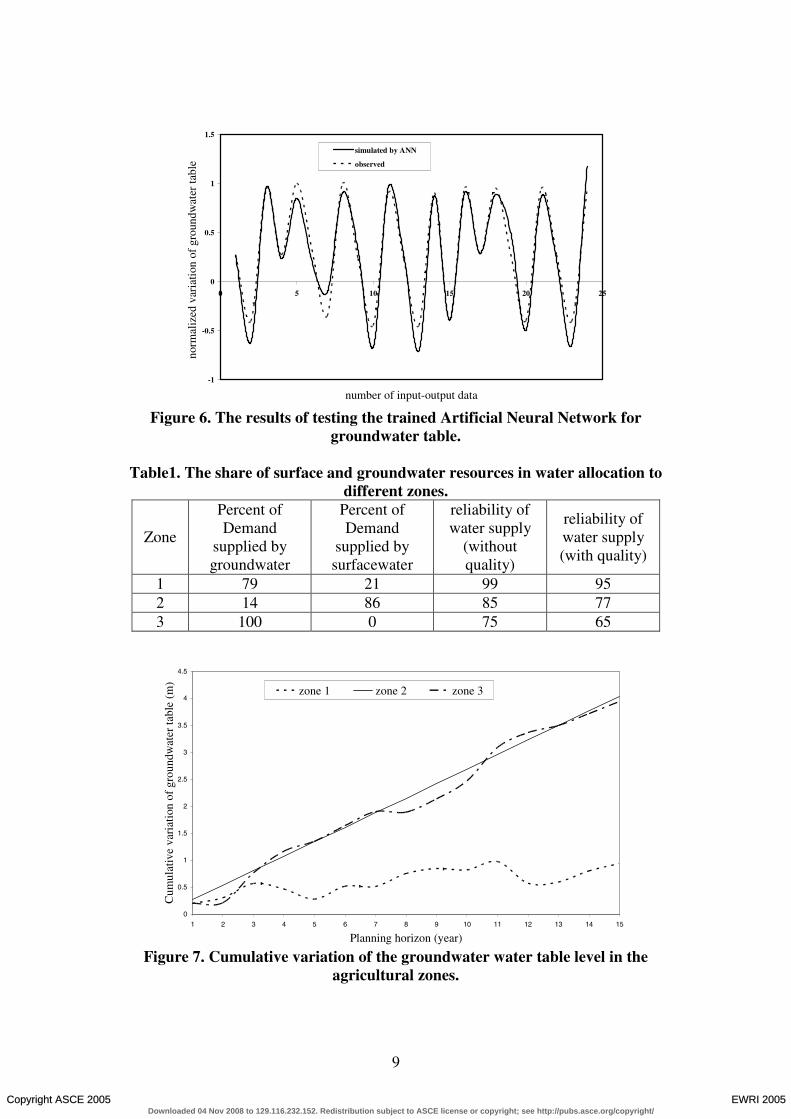
The developed ANN-based response functions can be used in the GA-base optimization models. Figure 6 shows the result of testing the trained ANN for simulating the groundwater table variations. As shown in this figure, the PMWINmodel can be replaced with the trained ANN.

Results and DiscussionIn this study, the conjunctive use policies for surface and groundwater resources are developed using a GA based optimization model. In this paper, the cumulative groundwater table variations in each zone, which has experienced atotal fluctuation of more than 20± meters in the last 20 years, is limited to 5±meters over the planning horizon (15 years). The relative weight of 1Z to 4Z are

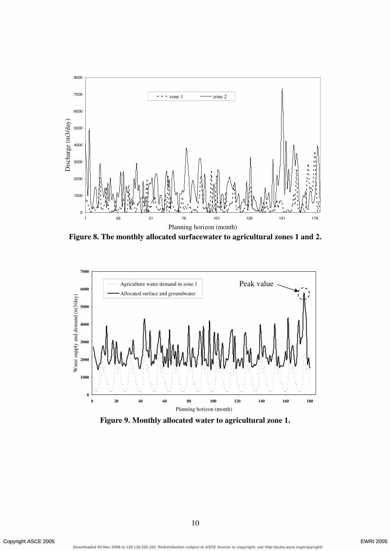
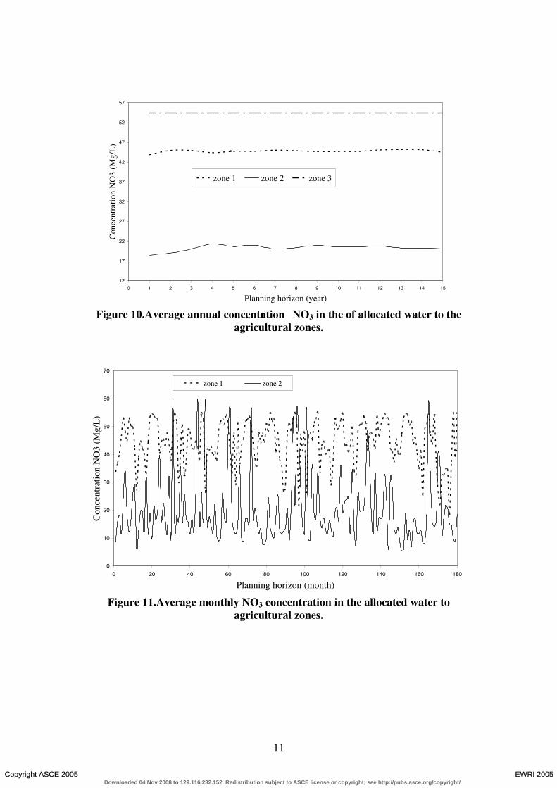
considered to be 30, 10, 35 and 25, respectively. Table 1 presents the reliability of the water supply to the agricultural water demands, and the share of ground and surface water resources allocation. Based on the results of this study, presented in Table 1, only 79 percent of the total water demand can be allocated and more than 64 percent of the allocated demand is supplied by the groundwater resources. Figure 7 shows the cumulative variation of groundwater table in the agricultural zones based on the optimal operating polices. In zone 2, less groundwater is extracted because of a lower concentration of water quality variable in the surfacewater of this zone (see Figures 8 and 11). As it can be seen in Figure 8, most of the allocated water to zone 2 is supplied from surface water resources due to the availability of the surface water and best water quality in this zone as well as to reduce the pumping cost. Figure 9 presents the total allocated water to zone 1. The peak value (in Figure 9 is due to the over allocating the groundwater to zone 1 to control the groundwater table in this zone. Based on the conjunctive use polices, the groundwater is allocated to zone 3 to control the increasing level of the groundwater table in this agricultural zone. Results of this study show that the proposed model can be effectively used for conjunctive use of surface and groundwater resources considering the water quality issues.


9

-1

-0.5

0

0.5

1

1.5

0 5 10 15 20 25

number of input-output data

norm

aliz

ed v

aria

tion

of

grou

ndw

ater

tabl

e

simulated by ANN

observed

Figure 6. The results of testing the trained Artificial Neural Network for groundwater table.

Table1. The share of surface and groundwater resources in water allocation to different zones.

Zone

Percent of Demand

supplied by groundwater

Percent of Demand

supplied bysurfacewater

reliability of water supply

(without quality)

reliability of water supply (with quality)

1 79 21 99 952 14 86 85 773 100 0 75 65

0

0.5

1

1.5

2

2.5

3

3.5

4

4.5

1 2 3 4 5 6 7 8 9 10 11 12 13 14 15

Planning horizon (year)

Cum

ulat

ive

vari

atio

n of

gro

undw

ater

tabl

e (m

)

zone 1 zone 2 zone 3

Figure 7. Cumulative variation of the groundwater water table level in the agricultural zones.


10

0

1000

2000

3000

4000

5000

6000

7000

8000

1 26 51 76 101 126 151 176

Planning horizon (month)

Dis

char

ge (

m3/

day)

zone 1 zone 2

Figure 8. The monthly allocated surfacewater to agricultural zones 1 and 2.

0

1000

2000

3000

4000

5000

6000

7000

0 20 40 60 80 100 120 140 160 180


Wat

er s

uppl

y an

d de

man

d (m

3/da

y)

Agriculture water demand in zone 1

Allocated surface and groundwater

Figure 9. Monthly allocated water to agricultural zone 1.

Peak value


11

12

17

22

27

32

37

42

47

52

57

0 1 2 3 4 5 6 7 8 9 10 11 12 13 14 15

Planning horizon (year)

Con

cent

rati

on N

O3

(Mg/

L)

zone 1 zone 2 zone 3

Figure 10.Average annual concentration NO3 in the of allocated water to the agricultural zones.

0

10

20

30

40

50

60

70

0 20 40 60 80 100 120 140 160 180


Con

cent

ratio

n N

O3

(Mg/

L)

zone 1 zone 2

Figure 11.Average monthly NO3 concentration in the allocated water to agricultural zones.


12

ReferencesFredericks, J., Labadie, J.W., and Altenhofen, J. (1998). “Decision support system

for conjunctive stream-aquifer management.”, J. of Water Resources Planning and Management, ASCE, 124(2), 69-78.

Gen, M. R. and Chang, L. (2000). Genetic Algorithm and Engineering Optimization, Wiley Europe Publication.

Hsing Chiang, Wen and Kinzelbach, W., “Manual 3D-Groundwater Modeling with PMWIN”, Springer, 2001

Hsu, K., Gupta, H. V., Sorooshian, S. (1995). “Artificial neural nerwork modeling of the rainfall-runoff process.” Water Resources Research, 31(10), 2517-2530.

Karamouz, M., Kerachian, R., and Zahraie, B. (2004). “Monthly water resources and irrigation planning: A case study of conjunctive use of surface and groundwater resources.” ASCE, J. of Irrig. and Drain. Eng., 130(5), 391-402.

Karamouz, M., Kerachian, R., Zahraie, Ba., and Zahraie, Be. (2002). “Conjunctive use of surface and groundwater resources.” Proceedings of ASCE Environmental and Water Resources Institute Conference, Roanoke, Virginia, May 19-22.

Karamouz, M., Rezapour Tabari, M.M., Kerachian, R. (2004). “Conjunctive Use of Surface and Groundwater Resources: Application of Genetic Algorithms and Neural Networks” Proceedings of ASCE Environmental and Water Resources Institute Conference, Salt Lake City- Utah.

Loaiciga, H. A., and Leipnik, R. B. (2001). “Theory of sustainable groundwater management: An urban case study.” Urban Water, 3, 217-228.

Maddock, T. (1974). “The operation of a stream-aquifer system under stochastic demands.” Water Resources Research, 10(1), 1-10.

Onta, P. R., Gupta, A. D., and Harboe, R. (1991). “Multi-site planning models for conjunctive use of surface and ground water resources.” J. of Water Resources Planning and Management, ASCE, 117(6), 662-678.

Yeh, W. W-G. (1992). “System analysis in groundwater planning and management.”J. of Water Resources Planning and Management, ASCE, 118(3), 224-237.


conjunctive use of surface and groundwater resources with

Documents