optimal algorithms for learning bayesian network ... · optimal algorithms for learning bayesian...
TRANSCRIPT

1/56
Optimal Algorithms for Learning Bayesian Network Structures:
Introduction and Heuristic Search
Optimal Algorithms for Learning Bayesian Network Structures:
Introduction and Heuristic Search
Changhe YuanUAI 2015 Tutorial
Sunday, July 12th, 8:30-10:20amhttp://auai.org/uai2015/tutorialsDetails.shtml#tutorial_1

2/56
About tutorial presenters
• Dr. Changhe Yuan (Part I)– Associate Professor of Computer Science at Queens College/City University of
New York – Director of the Uncertainty Reasoning Laboratory (URL Lab).
• Dr. James Cussens (Part II)– Senior Lecturer in the Dept of Computer Science at the University of York, UK
• Dr. Brandon Malone (Part I and II)– Postdoctoral researcher at the Max Planck Institute for Biology of Ageing

3/56
Bayesian networks
• A Bayesian Network is a directed acyclic graph (DAG) in which:– A set of random variables makes up the nodes in the network.– A set of directed links or arrows connects pairs of nodes.– Each node has a conditional probability table that quantifies the effects the
parents have on the node.
P(B) P(E)
P(N|A)
P(R|E)P(A|B,E)
4/56
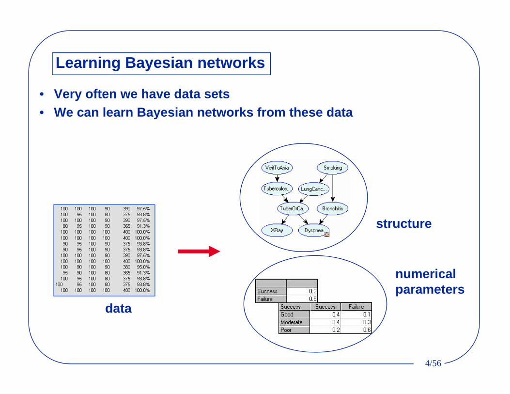
Learning Bayesian networks
• Very often we have data sets• We can learn Bayesian networks from these data
data
structure
numerical parameters

5/56
Major learning approaches
• Score-based structure learning– Find the highest-scoring network structure
» Optimal algorithms (FOCUS of TUTORIAL)» Approximation algorithms
• Constraint-based structure learning– Find a network that best explains the dependencies and
independencies in the data
• Hybrid approaches– Integrate constraint- and/or score-based structure learning
• Bayesian model averaging– Average the prediction of all possible structures

6/56
Score-based learning
• Find a Bayesian network that optimizes a given scoring function
• Two major issues– How to define a scoring function?– How to formulate and solve the optimization problem?

7/56
Scoring functions
• Bayesian Dirichlet Family (BD)– K2
• Minimum Description Length (MDL)• Factorized Normalized Maximum Likelihood (fNML)• Akaike’s Information Criterion (AIC)• Mutual information tests (MIT)• Etc.

8/56
• All of these are expressed as a sum over the individual variables, e.g.
• This property is called decomposability and will be quite important for structure learning.
BDeu
MDL
fNML
Decomposability
[Heckerman 1995, etc.]

9/56
Querying best parents
e.g.,
Naive solution: Search through all of the subsets and find the best
Solution: Propagate optimal scores and store as hash table.

10/56
POPS(X1|PA(X1))
Score pruning
• Theorem: Say PAi ⊂ PA’i and Score Xi|PAi Score X|PA’i . Then PA’iis not optimal for Xi.
• Ways of pruning: – Compare Score Xi|PAi and Score X|PA’i– Using properties of scoring functions without computing scores (e.g.,
exponential pruning)• After pruning, each variable has a list of possibly optimal parent
sets (POPS)– The scores of all POPS are called local scores
[Teyssier and Koller 2005, de Campos and Ji 2011, Tian 2000]

11/56
Number of POPS
1.00E+00
1.00E+01
1.00E+02
1.00E+03
1.00E+04
1.00E+05
1.00E+06
1.00E+07
1.00E+08
1.00E+09
1.00E+10Optim
al Paren
t Sets
Full Largest Layer Sparse
The number of parent sets and their scores stored in the full parent graphs (“Full”), the largest layer of the parent graphs in memory-efficient dynamic programming(“Largest Layer”), and the possibly optimal parent sets (“Sparse”).

12/56
Practicalities
• Empirically, the sparse AD-tree data structure is the best approach for collecting sufficient statistics.
• A breadth-first score calculation strategy maximizes the efficiency of exponential pruning.
• Caching significantly reduces runtime.
• Local score calculations are easily parallelizable.

13/56
Graph search formulation
• Formulate the learning task as a shortest path problem – The shortest path solution to a graph search problem corresponds to an optimal
Bayesian network
[Yuan, Malone, Wu, IJCAI-11]

14/56
Search graph (Order graph)
ϕ
1 2 3
1,2 1,3 2,3
1,2,3
4
1,4 2,4 3,4
1,2,4 1,3,4 2,3,4
1,2,3,4
Formulation: Search space: Variable subsetsStart node: Empty setGoal node: Complete setEdges: Add variableEdge cost: BestScore(X,U) for
edge UU{X}
3
2
4
[Yuan, Malone, Wu, IJCAI-11]

15/56
Search graph (Order graph)
ϕ
1 2 3
1,2 1,3 2,3
1,2,3
4
1,4 2,4 3,4
1,2,4 1,3,4 2,3,4
1,2,3,4
Formulation: Search space: Variable subsetsStart node: Empty setGoal node: Complete setEdges: Add variableEdge cost: BestScore(X,U) for
edge UU{X}Task: find the shortest path between start and goal nodes
2
1
4
31,3,4,2
[Yuan, Malone, Wu, IJCAI-11]

16/56
ϕ
A* search: Expands the nodes in the order of quality: f=g+h
g(U) = Score(U)h(U) = estimated distance to goal
A* algorithm
[Yuan, Malone, Wu, IJCAI-11]
h
1,2,3,4
010
Notation:g: g-costh: h-costRed shape-outlined: open nodesNo outline: closed nodes

17/56
414
ϕ
1 2 3
1,2,3,4
A* search: Expands the nodes in the order of quality: f=g+h
g(U) = Score(U)h(U) = estimated distance to goal4
g
h
[Yuan, Malone, Wu, IJCAI-11]
010
210
38
511
Notation:g: g-costh: h-costRed shape-outlined: open nodesNo outline: closed nodes
A* algorithm

18/56
ϕ
1 2 3
3,4
1,2,3,4
A* search: Expands the nodes in the order of quality: f=g+h
g(U) = Score(U)h(U) = estimated distance to goal
A* algorithm
4
g
h
[Yuan, Malone, Wu, IJCAI-11]
2,3
010
210
414
38
511
5/10 4/12 5/11
Notation:g: g-costh: h-costRed shape-outlined: open nodesNo outline: closed nodes
1,3

19/56
ϕ
1 2 3
1,2 1,3
1,2,3,4
A* search: Expands the nodes in the order of quality: f=g+h
g(U) = Score(U)h(U) = estimated distance to goal
A* algorithm
4g
h
[Yuan, Malone, Wu, IJCAI-11]
2,3 3,41,4
010
210
414
38
511
4/13 5/12 4/10 5/11
Notation:g: g-costh: h-costRed shape-outlined: open nodesNo outline: closed nodes
4/12

20/56
ϕ
1 2 3
1,2 1,3
A* search: Expands the nodes in the order of quality: f=g+h
g(U) = Score(U)h(U) = estimated distance to goal
A* algorithm
4g
[Yuan, Malone, Wu, IJCAI-11]
2,3 3,41,4
1,2,3,4
h
1,3,41,2,3
010
210
414
38
511
4/13 5/12 4/10 5/11
5/13 5/10
Notation:g: g-costh: h-costRed shape-outlined: open nodesNo outline: closed nodes
4/12

21/56
ϕ
1 2 3
1,2 1,3
A* search: Expands the nodes in the order of quality: f=g+h
g(U) = Score(U)h(U) = estimated distance to goal
A* algorithm
4g
[Yuan, Malone, Wu, IJCAI-11]
2,3 3,41,4
010
210
414
38
511
4/13 5/11
Notation:g: g-costh: h-costRed shape-outlined: open nodesNo outline: closed nodes
1,2,3,4
1,3,41,2,3
5/12 4/10
5/13 5/10
4/12
15/0

22/56
ϕ
1 2 3
1,2 1,3
A* search: Expands the nodes in the order of quality: f=g+h
g(U) = Score(U)h(U) = estimated distance to goal
A* algorithm
4g
[Yuan, Malone, Wu, IJCAI-11]
2,3 3,41,4
1,2,3
010
210
414
38
511
4/13 5/12 4/10 5/11
5/13
Notation:g: g-costh: h-costRed shape-outlined: open nodesNo outline: closed nodes
1,2,3,4
1,3,45/10
4/12
15/0

23/56
Simple heuristic
[Yuan, Malone, Wu, IJCAI-11]
A* search: Expands nodes in order of quality: f=g+h
g(U) = Score(U)h(U) = XV\U BestScore(X, V\{X})
h({1,3}):
32
14
ϕ
1 2 3
1,2 1,3
4
2,3 3,41,4
1,2,3,4
h

24/56
Properties of the simple heuristic• Theorem: The simple heuristic function h is admissible
– Optimistic estimation: never overestimate the true distance– Guarantees the optimality of A*
• Theorem: h is also consistent– Satisfies triangular inequality, yielding a monotonic heuristic– Consistency => admissibility– Guarantees the optimality of g cost of any node to be expanded
[Yuan, Malone, Wu, IJCAI-11]

25/56
BFBnB algorithm
ϕ
1 2 3
1,2 1,3 2,3
1,2,3
4
1,4 2,4 3,4
1,2,4 1,3,4 2,3,4
1,2,3,4
[Malone, Yuan, Hansen, UAI-11]
Breadth-first branch and bound search (BFBnB):• Motivation:
Exponential-size order&parent graphs
• Observation:Natural layered structure
• Solution:Search one layer at a time

26/56
BFBnB algorithm
Breadth-first branch and bound search (BFBnB):• Motivation:
Exponential-size order&parent graphs
• Observation:Natural layered structure
• Solution:Search one layer at a time
ϕ
1 2 3
1,2 1,3 2,3
1,2,3
4
1,4 2,4 3,4
1,2,4 1,3,4 2,3,4
1,2,3,4
[Malone, Yuan, Hansen, UAI-11]

27/56
BFBnB algorithm
ϕ
1 2 3 4
[Malone, Yuan, Hansen, UAI-11]

28/56
ϕ
1 2 3 41 2 3
1,2 1,3 2,3
4
1,4 2,4 3,4
[Malone, Yuan, Hansen, UAI-11]
BFBnB algorithm

29/56
1 2 3
1,2 1,3 2,3
4
1,4 2,4 3,41,2 1,3 2,3
1,2,3
1,4 2,4 3,4
1,2,4 1,3,4 2,3,4
ϕ
1 2 3 4
[Malone, Yuan, Hansen, UAI-11]
BFBnB algorithm

30/56
1,2 1,3 2,3
1,2,3
1,4 2,4 3,4
1,2,4 1,3,4 2,3,41,2,3 1,2,4 1,3,4 2,3,4
1,2,3,4
1 2 3
1,2 1,3 2,3
4
1,4 2,4 3,4
ϕ
1 2 3 4
[Malone, Yuan, Hansen, UAI-11]
BFBnB algorithm

31/56
Pruning in BFBnB
ϕ
1 2 3
1,3 2,3 1,4 2,4
1,2,4 1,3,4 2,3,4
1,2,3,4
• For pruning, estimate an upper bound solution before search– Can be done using anytime window A*
• Prune a node when f-cost > upper bound
[Malone, Yuan, Hansen, UAI-11]

32/56
Performance of A* and BFBnB
A comparison of the total time (in seconds) for GOBNILP, A*, and BFBnB. An “X” means that the corresponding algorithm did not finish within the time limit (7,200 seconds) or ran out of memory in the case of A*.

33/56
Drawback of simple heuristic
• Let each variable to choose optimal parents from all the other variables
• Completely relaxes the acyclic constraint
2
1
3
4
21
3 4
Bayesian network Heuristic estimation
Relaxation

34/56
Potential solution
• Breaking cycles to obtain a tighter heuristic
21
3 4
21
3 4
21
3 4
BestScore(1, {2,3,4})={2,3,4}+
BestScore(2, {1,3,4})={1,4}
BestScore(1, {2,3,4})+
BestScore(2, {3,4})={3}
BestScore(1, {3,4})={3,4}+
BestScore(2, {1,3,4})
min c({1,2})
[Yuan, Malone, UAI-12]

35/56
Static k-cycle conflict heuristic
• Also called static pattern database• Calculate joint costs for all subsets of non-overlapping static
groups by enforcing acyclicity within a group: {1,2,3,4,5,6} {1,2,3}, {4,5,6}
[Yuan, Malone, UAI-12]
1,2,3
1 2 3
1,2 1,3 2,3
ϕ
4,5,6
4 5 6
4,5 4,6 5,6
ϕ
h({1}) = gr({1})
gr

36/56
Computing heuristic value using static PD
• Sum costs of pattern databases according to static grouping
1,2,3
1 2 3
1,2 1,3 2,3
ϕ
4,5,6
4 5 6
4,5 4,6 5,6
ϕ
h({1,5,6}) = h({1})+h({5,6})
[Yuan, Malone, UAI-12]

37/56
Properties of static k-cycle conflict heuristic
• Theorem: The static k-cycle conflict heuristic is admissible
• Theorem: The static k-cycle conflict heuristic is consistent
[Yuan, Malone, UAI-12]

38/56
Enhancing A* with static k-cycle conflict heuristic
A comparison of the search time (in seconds) for GOBNILP, A*, BFBnB, and A* with pattern database heuristic. An “X” means that the corresponding algorithm did not finish within the time limit (7,200 seconds) or ran out of memory in the case of A*.

39/56
Learning decomposition
• Potentially Optimal Parent Sets (POPS)– Contain all parent-child relations
• Observation: Not all variables can possibly be ancestors of the others.
– E.g., any variables in {X3,X4,X5,X6} can not be ancestor of X1 or X2
[Fan, Malone, Yuan, UAI-14]

40/56
POPS Constraints
• Parent Relation Graph– Aggregate all the parent-child relations in POPS Table
• Component Graph– Strongly Connected Components (SCCs)– Provide ancestral constraints
{1, 2}
{3,4,5,6}
[Fan, Malone, Yuan, UAI-14]

41/56
POPS Constraints
• Decompose the problem– Each SCC corresponds to a
smaller subproblem
– Each subproblem can be solved independently.
{1, 2}
{3,4,5,6}
[Fan, Malone, Yuan, UAI-14]

42/56
POPS Constraints
• Recursive POPS Constraints– Selecting the parents for one of
the variables has the effect of removing that variable from the parent relation graph.
[Fan, Malone, Yuan, UAI-14]
43/56
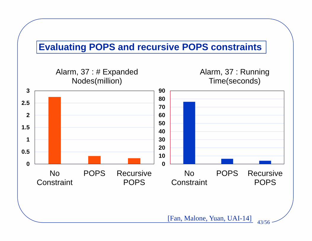
Evaluating POPS and recursive POPS constraints
0102030405060708090
NoConstraint
POPS RecursivePOPS
Alarm, 37 : Running Time(seconds)
0
0.5
1
1.5
2
2.5
3
NoConstraint
POPS RecursivePOPS
Alarm, 37 : # Expanded Nodes(million)
[Fan, Malone, Yuan, UAI-14]

44/56
Evaluating POPS and recursive POPS constraints
0
0.1
0.2
0.3
0.4
0.5
0.6
0.7
NoConstraint
POPS RecursivePOPS
Barley, 48: # Expanded Nodes(million)
0
0.5
1
1.5
2
2.5
3
NoConstraint
POPS RecursivePOPS
Barley, 48 : # Running Time(seconds)
[Fan, Malone, Yuan, UAI-14]

45/56
Evaluating POPS and recursive POPS constraints
0
100
200
300
400
500
600
NoConstraint
POPS RecursivePOPS
Soybean, 36 : # Running Time(seconds)
0
2
4
6
8
10
12
NoConstraint
POPS RecursivePOPS
Soybean, 36 : # Expanded Nodes(seconds)
[Fan, Malone, Yuan, UAI-14]

46/56
Grouping in static k-cycle conflict heuristic• Tightness of the heuristic highly depends on the grouping• Characteristics of a good grouping
– Reduce directed cycles between groups – Enforce as much acyclicity as possible
[Fan, Yuan, AAAI-15]

47/56
Existing grouping methods
• Create an undirected graph as skeleton– Parent grouping: connecting each variable to potentials parents in the best
POPS– Family grouping: use Min-Max Parent Child (MMPC) [Tsarmardinos et al. 06]
• Use independence tests in MMPC to estimate edge weights• Partition the skeleton into balanced subgraphs
– by minimizing the total weights of the edges between the subgraphs
[Fan, Yuan, AAAI-15]

48/56
Advanced grouping
• The potentially optimal parent sets (POPS) capture all possible relations between variables
• Observation: Directed cycles in the heuristic originate from the POPS
[Fan, Yuan, AAAI-15]

49/56
Parent relation graphs from all POPS
[Fan, Yuan, AAAI-15]

50/56
Parent relation graph from top-K POPS
K = 1 K = 2
[Fan, Yuan, AAAI-15]

51/56
Component grouping • : the size of the largest pattern database that can be created• Use parent grouping if the largest SCC in top-1 graph is already
larger than • Otherwise, use component grouping
– For K = 1 to maxi |POPS|i» Use top-K POPS of each variable to create a parent relation graph» If the graph has only one SCC or a too large SCC, return» Divide the SCCs into two or more groups by using a Prim-like algorithm
– Return feasible grouping of largest K
[Fan, Yuan, AAAI-15]

52/56
Parameter K
The running time and number of expanded nodesneeded by A* to solve Soybeans with different K.
[Fan, Yuan, AAAI-15]

53/56
Comparing grouping methods
[Fan, Yuan, AAAI-15]

54/56
• Formulation:– learning optimal Bayesian networks as a shortest path problem– Standard heuristic search algorithms applicable, e.g., A*, BFBnB– Design of upper/lower bounds critical for performance
• Extra information extracted from data enables– Creating ancestral graphs for decomposing the learning problem– Creating better grouping for the static k-cycle conflict heuristic
• Take home message: Methodology and data work better as a team!
• Open source software available from– http://urlearning.org
Summary

55/56
• NSF CAREER grant, IIS-0953723• NSF IIS grant, IIS-1219114• PSC-CUNY Enhancement Award• The Academy of Finland (COIN, 251170)
Acknowledgements
56/56
References• Xiannian Fan, Changhe Yuan. An Improved Lower Bound for Bayesian Network Structure Learning. In Proceedings
of the 29th AAAI Conference (AAAI-15). Austin, Texas. 2015.• Xiannian Fan, Brandon Malone, Changhe Yuan. Finding Optimal Bayesian Networks Using Constraints Learned
from Data. In Proceedings of the 30th Annual Conference on Uncertainty in Artificial Intelligence (UAI-14). Quebec City, Quebec. 2014.
• Xiannian Fan, Changhe Yuan, Brandon Malone. Tightening Bounds for Bayesian Network Structure Learning. In Proceedings of the 28th AAAI Conference on Artificial Intelligence (AAAI-14). Quebec City, Quebec. 2014.
• Changhe Yuan, Brandon Malone. Learning Optimal Bayesian Networks: A Shortest Path Perspective. Journal of Artificial Intelligence Research (JAIR). 2013.
• Brandon Malone, Changhe Yuan. Evaluating Anytime Algorithms for Learning Optimal Bayesian Networks. In Proceedings of the 29th Conference on Uncertainty in Artificial Intelligence (UAI-13). Seattle, Washington. 2013.
• Brandon Malone, Changhe Yuan. A Depth-first Branch and Bound Algorithm for Learning Optimal Bayesian Networks. IJCAI-13 Workshop on Graph Structures for Knowledge Representation and Reasoning (GKR'13). Beijing, China. 2013.
• Changhe Yuan, Brandon Maone. An Improved Admissible Heuristic for Learning Optimal Bayesian Networks. In Proceedings of the 28th Conference on Uncertainty in Artificial Intelligence (UAI-12). Catalina Island, CA. 2012.
• Brandon Malone. Learning optimal Bayesian networks with heuristic search. PhD Dissertation. Department of Computer Science and Engineering, Mississippi State University. July, 2012.
• Brandon Malone, Changhe Yuan. A Parallel, Anytime, Bounded Error Algorithm for Exact Bayesian Network Structure Learning. In Proceedings of the Sixth European Workshop on Probabilistic Graphical Models (PGM-12). Granada, Spain. 2012.
• Changhe Yuan, Brandon Malone and Xiaojian Wu. Learning Optimal Bayesian Networks Using A* Search. 22nd International Joint Conference on Artificial Intelligence (IJCAI-11). Barcelona, Catalonia, Spain, July 2011.
• Brandon Malone, Changhe Yuan, Eric Hansen and Susan Bridges. Memory-Efficient Dynamic Programming for Learning Optimal Bayesian Networks, 25th AAAI Conference on Artificial Intelligence (AAAI-11). San Francisco, CA. August 2011.
• Brandon Malone, Changhe Yuan, Eric Hansen and Susan Bridges. Improving the Scalability of Optimal Bayesian Network Learning with Frontier Breadth-First Branch and Bound Search, 27th Conference on Uncertainty in Artificial Intelligence (UAI-11). Barcelona, Catalonia, Spain, July 2011.