Engineering, 2014, 6, 773-788 Published Online November 2014 in SciRes. http://www.scirp.org/journal/eng http://dx.doi.org/10.4236/eng.2014.612075

How to cite this paper: Filho, O.S.S. (2014) Optimal Aggregate Production Plans via a Constrained LQG Model. Engineering, 6, 773-788. http://dx.doi.org/10.4236/eng.2014.612075

Optimal Aggregate Production Plans via a Constrained LQG Model Oscar S. Silva Filho

Center for Information Technology Renato Archer—CTI, Campinas, Brazil Email: oscar.salviano@cti.gov.br Received 27 August 2014; revised 25 September 2014; accepted 14 October 2014

Copyright © 2014 by author and Scientific Research Publishing Inc. This work is licensed under the Creative Commons Attribution International License (CC BY). http://creativecommons.org/licenses/by/4.0/

Abstract In this paper, a single product, multi-period, aggregate production planning problem is formu-lated as a linear-quadratic Gaussian (LQG) optimal control model with chance constraints on state and control variables. Such formulation is based on a classical production planning model devel-oped in 1960 by Holt, Modigliani, Muth and Simon, and known, since then, as the HMMS model [1]. The proposed LQG model extends the HMMS model, taking into account both chance-constraints on the decision variables and data generating process, based on ARMA model, to represent the fluctuation of demand. Using the certainty-equivalence principle, the constrained LQG model can be transformed into an equivalent, but deterministic model, which is called here as Mean Value Problem (MVP). This problem preserves the main properties of the original model such as con-vexity and some statistical moments. Besides, it is easier to be implemented and solved numeri-cally than its stochastic version. In addition, two very simple suboptimal procedures from sto-chastic control theory are briefly discussed. Finally, an illustrative example is introduced to show how the extended HMMS model can be used to develop plans and to generate production scena-rios.

Keywords Production Planning, Operations Management, Stochastic Models, Optimization, Forecasting

1. Introduction A production planning process requires a set of decisions used to match company’s industrial resources to the customer demand fluctuation. Among the first decisions to be made there is the development of aggregate pro-duction plan. The main objective of this plan is to determine aggregate levels of production, inventory and workforce in order to meet the expected demand for products within a planning horizon that usually ranges from

O. S. S. Filho

774

six months to one year. Once the plan is generated, constraints are imposed on the detailed production schedul-ing process allowing specify the proper amount of material resources needed to produce each product. Therefore, someone may say that the development of an efficient production plan is the first step to reducing costs with material resources of a company.

Due to uncertainties of the production environment, the aggregate plan must be constantly updated in order to provide efficient production targets for the short term planning process, see, e.g., [2]-[5]. As a consequence, no-sequential (i.e., static) stochastic optimization models are inappropriate to represent this kind of environment. The main reason is that these models do not take into account any new information available over the time-pe- riods about the current state of the production system [6]. Thus, sequential constrained stochastic optimization models, based on the theory of stochastic dynamic programming and optimal control theory, are the most-ap- propriate options for modeling this type of problem, see [2] and [7]-[10].

The objective of this paper is to develop a production plan from a well-structured sequential stochastic pro-duction planning model with chance-constraints on the decision variables. In this way, the classical aggregate production planning model developed by Holt, Modigliani, Muth and Simon—HMMS model, see [11]—is used as a pattern of reference. The HMMS model yields magnitude of production-rate, workforce level and net in-ventory per period that are optimal in that they are provided by minimizing the overall expected quadratic cost of running a production system. The idea is to propose an extension of the HMMS model to allow randomness in products’ demand and chance-constraints on decision variables. The sequential stochastic model follows the two steps: first step considers an equivalent state-space time-discrete LQG model with constraints on decision variables to represent the classical HMMS model. Additionally, the data generating process for demand fore-casting are incorporated into the model. Such a process is based on state-space Auto-Regressive Moving-Average (ARMA) model; see [12]. In the second step, a method, based on both mathematical programming and stochas-tic control theory, is applied to model in order to provide a sequential optimal production plan.

Due to particular features of the constrained LQG model—such as dimensionality, constraints on decision va-riables, and the stochastic nature of the system—this model is very difficult to be solved in an optimal closed- loop solution. This drawback means that classical optimal techniques of the stochastic mathematical program-ming can not be applied directly to the problem [13]. Thus, in order to reduce the complexity of the stochastic problem and, as well as, to make it computationally easier to solve, suboptimal approaches provided from sto-chastic control theory should be considered for practical applications, see, e.g., [9] [13]-[15]. Note that the li-near-Gaussian nature of the system and the quadratic criterion are also particular features of the model that allow the application of the certainty-equivalence principle [16]. From this principle, the stochastic model can be con-verted into a deterministic equivalent model. In such an equivalent model, all stochastic variables are set equal to their expected values (i.e., their first statistic moments). This model is usually known as Mean Value Model. The main advantage of this model is that, besides being easier to be solved, some mathematical and statistical properties of the original model are preserved, see [14].

The paper is organized as follows: Section 2 introduces an aggregate production planning problem based on the HMMS. The cost components of the original HMMS model are appropriately arranged to guarantee the con-sistency with the state-space pattern of the LQG model. Additionally, an input-output ARMA model, which is used as data generation process of demand, is transformed into a state-space format and attached to the LQG formulation. As a result, an extended state-space stochastic optimization model with constraints on decision va-riables is formulated. In Section 3, an equivalent deterministic optimization model is developed from the appli-cation of the certainty-equivalence principle. Two very simple sub-optimal approaches are used to solve the model. At last, Section 4 introduces an illustrative example to demonstrate the applicability of the model.

2. The HMMS Model in the State-Space Format In this section, the aggregate production planning problem, described by the classical HMMS model, is placed into space-state format in order to represent an equivalent LQG model with constraints on the decisions va-riables.

2.1. Basic Notation 1) Aggregate variables:

• kD denotes the demand for a family of products (i.e. the level of aggregate sales during period k ). It is as-

O. S. S. Filho

775

sumed to be a stationary random variable, being approximated by a normal distribution function with meanˆ

kD and finite variance 2 0D DV σ= ≥ . The assumption of normality is based on the Law of Large Number [17]. Such a law can be interpreted here as follows: the sum of different patterns of probability distribution functions, which are related to different products of the same family, can be approximated by a normal dis-tribution to represent this family. It is worth realizing that the probability distribution function of the demand usually depends on the type of the production process. For instance, considering a make-to-stock production process, where the evolution of demand is usually stationary over the periods, a normal distribution function, with mean and variance given, is statistically a good alternative to model the fluctuation of demand; see [18] for more details.

• kI denotes the amount of net inventory level at the beginning of period k . This variable takes values from a dynamic balance system that depends linearly on the demand fluctuation. Based on the property of a nor-mal stochastic process which says that the resulting linear transformation of a sequence of normal random variables is also a normal random variable (see [17]) is possible to consider that the inventory variable fol-lows a normal process with mean kI and variance 0I

kV ≥ . • kP denotes the rate of aggregate production capacity during the period k , being a decision variable to the

problem. Note that if, for instance, the inventory balance system is running under a closed-loop control scheme, then the production rate depends on the net inventory level for each period k , and, as a conse-quence, this rate must also be understood as being a random variable. Furthermore, if this dependence is li-near, then the probability distribution function of the production variable will be similar and proportional to the distribution function of the inventory variable; see this feature of the stochastic process in [7].

• kW denotes the amount of the regular workforce used in the period k . This variable is assumed here inde-pendent of endogenous and exogenous factors that influence the environment of the company. Indeed, there is a set point level for regular workforce denoted here as kW . Thus, any excess in the levels of fluctuation of demand, involving an increase in the production rate kP , will be dealt with a policy of the use of temporary labor or overtime. This variable is assumed to be essentially deterministic.

• 1k k kW W −∆ = − denotes workforce changes between the subsequent periods 1k − and k . It is a determi-nistic decision variable that provides the number of employees to be included or removed from the work-force level between two adjacent periods.

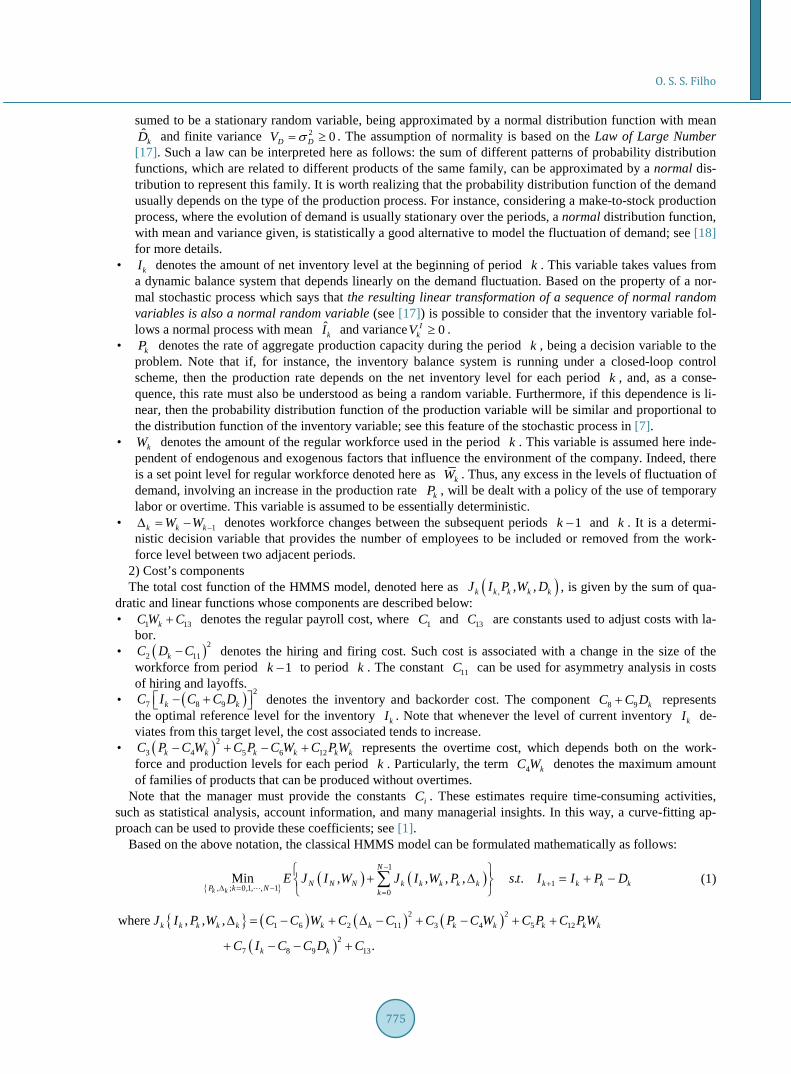
2) Cost’s components The total cost function of the HMMS model, denoted here as ( ), , ,k k k k kJ I P W D , is given by the sum of qua-

dratic and linear functions whose components are described below: • 1 13kC W C+ denotes the regular payroll cost, where 1C and 13C are constants used to adjust costs with la-

bor. • ( )2

2 11kC D C− denotes the hiring and firing cost. Such cost is associated with a change in the size of the workforce from period 1k − to period k . The constant 11C can be used for asymmetry analysis in costs of hiring and layoffs.

• ( ) 27 8 9k kC I C C D − + denotes the inventory and backorder cost. The component 8 9 kC C D+ represents

the optimal reference level for the inventory kI . Note that whenever the level of current inventory kI de-viates from this target level, the cost associated tends to increase.

• ( )23 4 5 6 12k k k k k kC P C W C P C W C P W− + − + represents the overtime cost, which depends both on the work-

force and production levels for each period k . Particularly, the term 4 kC W denotes the maximum amount of families of products that can be produced without overtimes.

Note that the manager must provide the constants iC . These estimates require time-consuming activities, such as statistical analysis, account information, and many managerial insights. In this way, a curve-fitting ap-proach can be used to provide these coefficients; see [1].

Based on the above notation, the classical HMMS model can be formulated mathematically as follows:

( ) ( )

1

1, ; 0,1, , 1 0Min , , , , . .

k k

N

N N N k k k k k k k k kP k N kE J I W J I W P s t I I P D

−

+∆ = − =

+ ∆ = + −

∑

(1)

( ) ( ) ( )( )

2 21 6 2 11 3 4 5 12

27 8 9 13

where , , ,

.

k k k k k k k k k k k k

k k

J I P W C C W C C C P C W C P C P W

C I C C D C

∆ = − + ∆ − + − + +

+ − − +

O. S. S. Filho

776

Note that the inventory balance equation given in the problem (1) is a stochastic process. Thus, the inventory variable is a random variable and, as a consequence, the model (1) represents a stochastic optimization problem. Therandomness explains the use of the mathematical expectation operator .E in the criterion. It is assumed that the initial inventory and workforce levels are known and given, respectively, by 0I and 0W . The level of

1W− is set equal to 0.

2.2. The Constrained HMMS Model As can be noted from problem (1), the classical formulation of HMMS model does not explicitly take into ac-count constraints on the decision variables; see also [1]. Indeed, any significant change in the levels of the deci-sion variables will be penalized directly in the criterion ( )kJ ⋅ . As a consequence, such criterion must be able to cover a sufficiently long span of time to ensure full recognition of the changes of these variables.

In this section, the HMMS model is modified in order to consider constraints on the inventory, production and workforce variables explicitly in the formulation. It is a consensus that the use of physical constraints explicitly in the model makes it more realistic for practical applications; see e.g. [16] and [19]. Based on this, the original formulation of problem (1) will be reformulated to include constraints on decision variables. Thus, assuming that it is possible to set lower and upper bounds for each decision variable of the model, and also to include a workforce balance constraint, the reformulated model is described as follows: finding a non-negative optimal policy, which includes both production rates ( ) ; 0,1, , 1

kk P kP I k Nµ= = − and workforce changes

; 0,1, , 1k k N∆ = − , to optimize the following production planning problem:

( ) ( )

( )( )

1

, ; 0,1, , 1 0

1 0

1 0

Min , , , ,

. . , given , given

Prob.

Prob.

0

k k

N

N N N k k k k kP k N k

k k k k

k k k

k k k

k k k

k k

k

E J I W J I P W

s t I I P D IW W W

I I I

P P P

W W

α

β

ω

−

∆ = − =

+

+

+ ∆

= + −

= + ∆

≤ ≤ ≥

≤ ≤ ≥

≤ ≤

− ≤

∑

.k kω∆ ≤

(2)

where kI and kI denote lower and upper bounds on the inventory variable; kP and kP denote lower and upper bounds of the production variable; and kW is the upper boundary related to the size of regular workforce plus overtime. Note that the parameter kω denotes the maximum amount of workforce change, which is esti-mated for each period k.

The optimal production policy ( ) ; 0,1, , 1kk P kP I k Nµ= = − is assumed to depend on the inventory

variable kI for each period k of the planning horizon. Since kI is a random variable, the variable kP will also have a random behavior. Such dependence follows a mathematical structure that is given by the function

( )kPµ ⋅ . If ( )

kPµ ⋅ has a linear structure, the probability distribution of the production variable kP will be similar to the probability distribution of the inventory variable kI . Thus, since the inventory variable is assumed here to be a normal distribution with known first and second statistics moments, it follows then that the produc-tion variable will also be normally distributed with known expectation kP and standard deviation

2 0kV ≥ . It is interesting to observe that the randomness of the inventory and production variables makes them prob-

abilistic variables, and so to ensure that their physical boundaries are no violated, they must be taken as chance- constraints. Then, probabilistic indexes of inventory and production constraints, which are given respectively by α and β , are used to express the user’s expectation for the nonviolation of these constraints. These indexes vary within the interval [ )0,1 , and each one of them has its specific practical interpretation. For example, the index α is usually interpreted as the level of the customer satisfaction. Indeed, if the manager chooses α close to 1 means that he wants to meet the demand for complete, whenever it occurs. For instance, for 0.95α ≥

O. S. S. Filho

777

means that the manager expects to deliver the products on time at least 95% of the time. In order to guarantee a high level of customer satisfaction, the manager must adopt a safety stock policy that allows ready delivery. In short, varying α in the range [ )0,1 , it is possible to analyze different production scenarios based on safety stock policies, which imply in greater or smaller level of customer's satisfaction. Finally, note that the index β is used here to represent the productivity degree of the production process. This index is related to the produc-tion capacity required at each period of the planning horizon. The idea is to guarantee that unexpected orders, which may occur during a given period k , can be promptly attended; avoiding, thus, the occurrence of backor-der; see [20].

2.3. The Constrained HMMS Model in State-Space Format The constrained HMMS model (2) is placed into an equivalent state-space linear-quadratic Gaussian model. For such, the variables of the HMMS model are considered as state and control variables, that is, 1

k kx I= and 2k kx W= denote the state variables, and 1

k ku P= and 2k ku = ∆ denote the control (or input) variables. Based

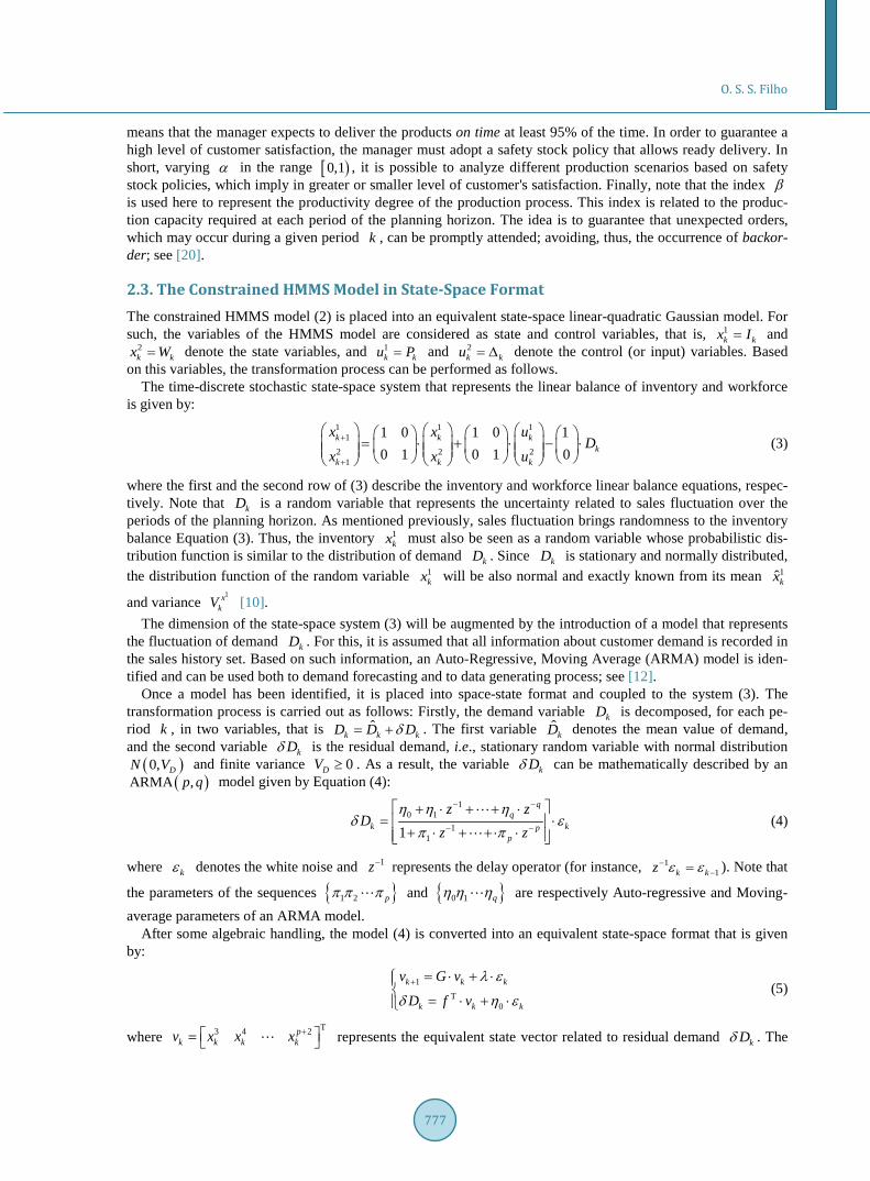
on this variables, the transformation process can be performed as follows. The time-discrete stochastic state-space system that represents the linear balance of inventory and workforce

is given by: 1 1 1

12 2 2

1

1 0 1 0 10 1 0 1 0

k k kk

k k k

x x uD

x x u+

+

= ⋅ + ⋅ − ⋅

(3)

where the first and the second row of (3) describe the inventory and workforce linear balance equations, respec-tively. Note that kD is a random variable that represents the uncertainty related to sales fluctuation over the periods of the planning horizon. As mentioned previously, sales fluctuation brings randomness to the inventory balance Equation (3). Thus, the inventory 1

kx must also be seen as a random variable whose probabilistic dis-tribution function is similar to the distribution of demand kD . Since kD is stationary and normally distributed, the distribution function of the random variable 1

kx will be also normal and exactly known from its mean 1ˆkx

and variance 1x

kV [10]. The dimension of the state-space system (3) will be augmented by the introduction of a model that represents

the fluctuation of demand kD . For this, it is assumed that all information about customer demand is recorded in the sales history set. Based on such information, an Auto-Regressive, Moving Average (ARMA) model is iden-tified and can be used both to demand forecasting and to data generating process; see [12].

Once a model has been identified, it is placed into space-state format and coupled to the system (3). The transformation process is carried out as follows: Firstly, the demand variable kD is decomposed, for each pe-riod k , in two variables, that is ˆ

k k kD D Dδ= + . The first variable ˆkD denotes the mean value of demand,

and the second variable kDδ is the residual demand, i.e., stationary random variable with normal distribution ( )0, DN V and finite variance 0DV ≥ . As a result, the variable kDδ can be mathematically described by an

( )ARMA ,p q model given by Equation (4): 1

0 11

11

qq

k kpp

z zD

z zη η η

δ επ π

− −

− −

+ ⋅ + + ⋅= ⋅

+ ⋅ + + ⋅ ⋅

(4)

where kε denotes the white noise and 1z− represents the delay operator (for instance, 11k kz ε ε−−= ). Note that

the parameters of the sequences 1 2 pπ π π and 0 1 qη η η are respectively Auto-regressive and Moving- average parameters of an ARMA model.

After some algebraic handling, the model (4) is converted into an equivalent state-space format that is given by:

1T

0

k k k

k k k

v G v

D f v

λ ε

δ η ε+ = ⋅ + ⋅

= ⋅ + ⋅

(5)

where T3 4 2p

k k k kv x x x + = represents the equivalent state vector related to residual demand kDδ . The

O. S. S. Filho

778

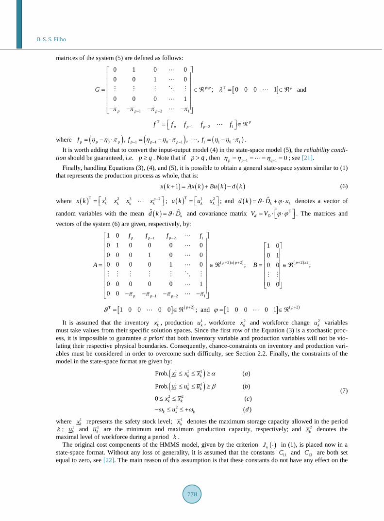
matrices of the system (5) are defined as follows:

[ ]T

1 2 1

0 1 0 00 0 1 0

; 0 0 0 10 0 0 1

pxp p

p p p

G λ

π π π π− −

= ∈ℜ = ∈ℜ − − − −

and

T1 2 1

pp p pf f f f f− − = ∈ℜ

where ( ) ( ) ( )0 1 1 0 1 1 1 0 1, , , p p p p p pf f fη η π η η π η η π− − −= − ⋅ = − ⋅ = − ⋅ . It is worth adding that to convert the input-output model (4) in the state-space model (5), the reliability condi-

tion should be guaranteed, i.e. p q≥ . Note that if p q> , then 1 1 0p p qη η η− += = = = ; see [21]. Finally, handling Equations (3), (4), and (5), it is possible to obtain a general state-space system similar to (1)

that represents the production process as whole, that is:

( ) ( ) ( ) ( )1x k Ax k Bu k d k+ = + − (6)

where ( )T 1 2 3 2pk k k kx k x x x x + = ; ( )T 1 2

k ku k u u = ; and ( ) ˆk kd k Dϑ ϕ ε= ⋅ + ⋅ denotes a vector of

random variables with the mean ( )ˆ ˆkd k Dϑ= ⋅ and covariance matrix T

DV V ϕ ϕ = ⋅ ⋅ d . The matrices and vectors of the system (6) are given, respectively, by:

( ) ( ) ( )

1 2 1

2 2 2 2

1 2 1

1 00 1 0 0 0 0 1 00 0 0 1 0 0 0 10 0 0 0 1 0 ; ;0 0

0 0 0 0 0 1 0 00 0

p p p

p x p p x

p p p

f f f f

A B

π π π π

− −

+ + +

− −

= ∈ℜ = ∈ℜ

− − − −

[ ] ( )2T 1 0 0 0 0 pϑ += ∈ℜ ; and [ ] ( )21 0 0 0 1 pϕ += ∈ℜ

It is assumed that the inventory 1kx , production 1

ku , workforce 2kx and workforce change 2

ku variables must take values from their specific solution spaces. Since the first row of the Equation (3) is a stochastic proc-ess, it is impossible to guarantee a priori that both inventory variable and production variables will not be vio-lating their respective physical boundaries. Consequently, chance-constraints on inventory and production vari-ables must be considered in order to overcome such difficulty, see Section 2.2. Finally, the constraints of the model in the state-space format are given by:

( )( )

1 1 1

1 1 1

2 2

2

Prob. ( )

Prob. ( )

0 ( )

( )

k k k

k k k

k k

k k k

x x x a

u u u b

x x c

u d

α

β

ω ω

≤ ≤ ≥

≤ ≤ ≥

≤ ≤

− ≤ ≤ +

(7)

where 1kx represents the safety stock level; 1

kx denotes the maximum storage capacity allowed in the period k ; 1

ku and 1ku are the minimum and maximum production capacity, respectively; and 2

kx denotes the maximal level of workforce during a period k .

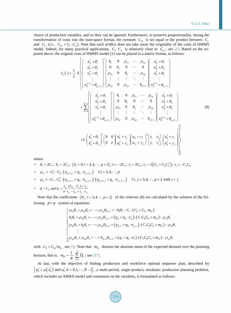
The original cost components of the HMMS model, given by the criterion ( )kJ ⋅ in (1), is placed now in a state-space format. Without any loss of generality, it is assumed that the constants 11C and 13C are both set equal to zero, see [22]. The main reason of this assumption is that these constants do not have any effect on the

O. S. S. Filho

779

choice of production variables, and so they can be ignored. Furthermore, to preserve proportionality, during the transformation of costs into the state-space format, the constant 12C is set equal to the product between 3C and 4C (i.e., 12 3 4C C C= ⋅ ). Note that such artifice does not take away the originality of the costs of HMMS model. Indeed, for many practical applications, 3 4C C⋅ is relatively close to 12C ; see [1]. Based on the ex-posed above, the original costs of HMMS model (1) can be placed in a matrix format, as follows:

( )

T1 11 13 11 1

2 222 2

3 313 3 33 3

2 21 3 22 2

11

22

00 0 0

1 02

0

pN N

N N

pk N N

p pp p pN p N p

N

N

hx xhx x

hJ E x x

hx x

xx

ρ ρθ θθ θ

ρ ρθ θ

ρ ρθ θ

θθ

+ +++ +

+ + + + ⋅ = ⋅ + + + +

++

+

T 11 13 1 1

22 21

3 313 3 33 3

0

2 21 3 22 2

T11

22

00 0 0

0

0

0 0 2

p N

NN

pN Nk

p pp p pN p N p

k

k

h xh x

hx x

hx x

x

x

ρ ρ θθ

ρ ρθ θ

ρ ρθ θ

θ

θ

−

=

+ +++ +

+ + + + + +

++ ⋅ +

∑

T1 11 1 1 11 3

2 23 22 22 2

.0

k i k

ik k

u u ur rr re uu u

γ γ γγγ γ

+ + + ⋅ ++ +

(8)

where • ( )2

1 7 2 2 2 1 3 2 2 3 4 3 3 42 ; 2 ; 0, 3, 4, , 2 ; 2 ; 2 ; 2 ; ih C h C h i p e C r C r C C C r C C= = = = + = − = = + = −

• ( )1 7 9 3 0 3 3, 4, ,j p i p iC C j pρ η η π+ − + −= − ⋅ ⋅ + ⋅ ∀ =

• ( ) ( )27 9 3 0 3 3 0 3 , 3, 4, , 2 with ij p i p i p j p jC C i j p i jρ η η π η η π+ − + − + − + −= − ⋅ ⋅ + ⋅ ⋅ + ⋅ ∀ = + <

• ( )11 6 1 121 8 2

11 12 11 22

andr C C r

Ce r r r r

θ θ⋅ − +

= =⋅ − + ⋅

Note that the coefficients , 3, 4 , 2i i pθ = + of the criterion (8) are calculated by the solution of the fol-lowing p p× system of equations:

( )( ) ( )( ) ( )

( ) ( )

13 3 14 4 1 2 1 1 7 8 9

3 3 34 4 3 2 0 7 8 9 13 1

34 3 4 4 4 2 1 0 1 7 8 9 14 1

3 3 4 4 2 2 1 0 1 7 8 9 1 1

p P D

p P p p D

p P p p D

p p p P D p

h C C C m

h C C C m

h C C C m

h C C C m

ρ θ ρ θ ρ θ θ

θ ρ θ ρ θ η η π ρ θ

ρ θ θ ρ θ η η π ρ θ

ρ θ ρ θ θ η η π ρ θ

+

+

+ − −

+ +

+ + + = − − ⋅ + ⋅

+ + + = + ⋅ ⋅ + − + + + = + ⋅ ⋅ + − + + + = + ⋅ ⋅ + −

with 9 8 DC C m= , see [1]. Note that Dm denotes the absolute mean of the expected demand over the planning

horizon, that is, 1

1 ˆN

D kk

m DN =

= ⋅∑ ; see [17].

At last, with the objective of finding production and workforce optimal sequence plan, described by

( ) 1 1 2 and ; 0,1, , 1k k ku x u k Nµ= = − , a multi-period, single-product, stochastic production planning problem,

which includes an ARMA model and constraints on the variables, is formulated as follows:

O. S. S. Filho

780

( )( ) ( ) ( ) ( ) ( ) ( ) ( ) ( )

( ) ( ) ( ) ( )( )( )

1T T T T

0

0

1

1

2 2

2

1Min 22

. . 1 ; given.

Prob.

Prob.

0

.

N

u k k

k k k

k k k

k k

k k k

E x N Hx N x k Hx k x k Eu k u k Ru k

s t x k Ax k Bu k d k x

x x x

u u u

x x

u

α

β

ω ω

−

=

+ + + + = + −

≤ ≤ ≥

≤ ≤ ≥

≤ ≤

− ≤ ≤ +

∑

(9)

The problem (9) is an extended version of the HMMS model, and it also belongs to the class of the linear, quadratic Gaussian model with constraints on state and control variables, see [13] and [16]. The main advantage is that it can be employed to model and optimize a wide variety of management problems in a unified format, see for instance [7] [9] [15] [19] [22] and [23]. The next section discusses the solution of the problem (9) by mean of two suboptimal approaches of the control theory, which are of simple implementation.

3. The Mean Value Problem Certain characteristics, such as the stochastic nature, constraints on decision variables and high dimensionality, make impossible to provide a true optimal solution (i.e. a close-loop solution) for the problem (9). The classical approach known as stochastic dynamic programming cannot be applied because the curse of dimensionality [13], which means that this approach requires an enormous computational effort to solve large-scale problems. Be-cause of these difficulties, suboptimal approaches become interesting alternatives, particularly in reason of the smallest computational effort that such techniques usually offer for practical applications; see [13] [14] and [15].

There is a wide variety of suboptimal approaches to deal with stochastic problems as described by problem (9). Many of them depend on the certainty-equivalence principle. Such principle establishes that all random variables of a stochastic problem can be replaced by their respective first statistical moments; see [14]. Base on this principle, the problem (9) can be transformed in an equivalent deterministic problem, denoted here as Mean Value Problem (MVP). This transformation process is facilitated by some features of the original problem, i.e.: 1) the linearity of the system (6); 2) the normal stochastic nature of the inventory balance equation, given in (3); and 3) the convexity of the functional criterion (8) that is explained by the quadratic nature of the cost of HMMS model, given in (1). As will be seen bellow, these features allow the immediate use of the certainty-equivalence principle.

3.1. The Transformation Process Having been assumed previously that the demand ( )d k is normally distributed, then it is possible to conclude that the statistical behaviour of the linear inventory system given in (6) follows a normal process. This charac- teristic means that the probability distribution function of inventory, given by 1,x k

Φ , can be precisely computed

from (6) by mean of the determination of its respective mean and variance equations; see [20]. These two statis-tical moments allow transforming the stochastic problem (9) into a Mean Value Problem (MVP).

The first step for converting the stochastic problem (9) to an equivalent MVP is to determine the mean and variance of the state variables of the system (6). However, it is important to bear in mind that the inventory variable 1

kx is the only random variable of the vector ( )x k , with mean 1 1ˆk kE x x= and standard deviation

( )1 Dxk kσ σ= ⋅ . As a result, the mean vector ( )x k and the covariance matrix ( )x kΩ of the system (6) are

given as follows:

( ) ( )

( ) ( ) ( )( )

( ) ( )1

T T 1 2 3 2 1 2 3 2 2

2

T 2 2

ˆ ˆ ˆ ˆ ˆ ,

0 0

.0 0 0

p p pk k k k k k k k

xp p

x

x k E x k E x x x x x x x x

k

E x k x k k

σ

+ + +

+ × +

= = = ∈ℜ

= Ω = ∈ℜ

(10)

O. S. S. Filho

781

Note that the other state variables (i.e., 1 2 3 2, , , , px x x x + ) of the system (6) are essentially deterministic, then only to guarantee the uniformity of the notation it will be considered here that

ˆ 0; 2,3,..., 2ii ik k x

x x and i pσ= = ∀ = + .

Since the control variable ( )u k depends on the state variable ( )x k , it can be completely defined by its

mean ( ) ( ) u k E u k= and covariance ( ) ( ) ( ) ( )T 2 2uE u k u k k ×= Ω ∈ℜ . Note also that the mean and cova-

riance of the demand variable are given respectively by ( ) ( ) ˆ ˆkd k E d k Dϕ= = ⋅ and ( ) 2 T

d Dk σ ϕ ϕ Ω = ⋅ ⋅ ,

with ϕ∈ p 2ϕ +∈ℜ , as discussed previously in Section 2.3.2. Based on these statistics, the criterion (8) and the linear system (6) can be promptly converted to a determinis-

tic equivalent pattern [20]. Another important transformation is to convert the probabilistic constraints (7.a) and (7.b) in equivalent deterministic inequalities. Thus, from (7.a) follows that:

( ) ( ) ( )1 11 1 1 1 1 1

, ,ˆProb. k k k k k x x k

x x x x x kαα σ α−≥ ≥ ⇔ ≥ = + ⋅Φ (11)

and,

( ) ( ) ( )1 11 1 1 1 1 1

, ,ˆProb. k k k k k x x k

x x x x x kαα σ α−< ≥ ⇔ ≤ = − ⋅Φ (12)

where ( )11,

.x k−Φ denotes the inverse probability distribution function of the inventory variable, which depends

on the service level α . Proceeding in a similar way, follows that the probabilistic constraint (7.b) becomes:

( )1 1 1 1 1 1, ,ˆProb. 2 1k k k k k ku u u u u uβ ββ≤ ≤ ≥ ⋅ − ⇔ ≤ ≤ (13)

where ( ) ( )1 11 1 1

, ,k k u u ku u kβ σ β−= + ⋅Φ ; ( ) ( )1 1

1 1 1, ,k k u u k

u u kβ σ β−= − ⋅Φ ; and ( )11,

.u k−Φ denotes the inverse probabil-

ity distribution function of the production variable, which depends on the production capacity reliability level, i.e., the probabilistic index β .

At last, it is important to observe that the state variables related to the ARMA model (i.e, 3 4 2ˆ ˆ ˆ, , , pk k kx x x + )

are totally unconstrained. This feature means that such variables can evolve freely along the planning horizon without any control.

After all these transformations, the Mean Value Problem can be formulated as follows:

( )( ) ( ) ( ) ( ) ( ) ( ) ( ) ( )

( ) ( ) ( ) ( ) ( )

1T T T T

ˆ 0

1 20 0

1 1 1, ,

1 1 1, ,

2 2

1ˆ ˆ ˆ ˆ ˆ ˆ ˆ ˆMin 22

ˆˆ ˆ ˆ ˆ ˆ ˆ. . 1 ; 0 0 0 is given

ˆ

ˆ

ˆ 0ˆ

N

u k k

k k k

k k k

k k

k

x N Hx N x k Hx k x k Eu k u k Ru k

s t x k x k u k d k x x x

x x x

u u u

x x

α α

β β

ω

−

=

+ + ⋅ + + = + ⋅ + =

≤ ≤

≤ ≤

≤ ≤

− ≤

∑

2 .k ku ω≤ +

(14)

It is worth mentioning that the problem (14) allows not only to provide an optimal aggregate production plan, but also to help the manager to get important insights about the use of the aggregate resources. Indeed, from varying some parameters of the problem (14), it is possible to analyse different scenarios related to an inven-tory-production process. For example, comparing optimal inventory, production and workforce trajectories, de-veloped from different scenarios analysis, the manager can realise how the future will be like in terms of the re-order cycle for a given product. The prior knowledge of all possible reorder points allows that some actions can be in advance taken to replenish the inventory levels, and, thus, to prevent against the possibility of stock out. These actions can be understood as an attempt to meet future demand for aggregate products, and also to prevent against unexpected events, such as, for instance, delays and machines breakdowns.

O. S. S. Filho

782

3.2. Two Simple Suboptimal Approaches Two simple suboptimal approaches, known in the literature as Open-loop No-updating and Open-Loop Updat-ing [13], can be combined with quadratic programming algorithms for solving (14), and so generating a sequen-tial optimal plan. These approaches are briefly described below. • The Open-Loop No-updating (OLN) approach applied to (14) provides an optimal production policy

( ) ˆ , 0,1, , 1u k k N= − that is entirely conditioned on initial information. Even if further information be-comes available, these initially computed policies are enacted up to the end of the time horizons,” see [15]. This characteristic means that OLN procedure provides an optimal sequence ( ) ( ) ( ) ˆ ˆ ˆ0 , 1 , , 1u u u N − that depends only on the initial state of the system (6), i.e., ( )ˆ 0x . Thus, any available information on the state of the system is completely ignored for period 0k > . Consequently, the OLN approach does not take into ac-count any feedback scheme in its strategy of providing a feasible solution for the problem (14).

• The Open-Loop Updating (OLU) approach is very similar to the OLN, except that optimal policies are al-ways recomputed as soon as new information about the state of the system becomes available [15]. In fact, for each new period [ ]0, 1k N∈ − , whenever the current state of the system ( )x k is measured, it is as-sumed to be a new-initial state to solve the problem (14) from the current period k to the end-period N . As a result, the optimal sequence ( ) ( ) ( ) ˆ ˆ ˆ, 1 , , 1u k u k u N− − is provided. From this sequence, only the first vector, i.e. ( ) ( )ˆ ˆu k u k∗ = , is applied to the system (6), while the others are completely ignored. Note that this approach must be repeated N times in order to provide optimal control policy for the problem (14).

Both OLN and OLU approaches can be used to develop production scenarios. These scenarios are useful for managers getting insights on the use of the resources of the company. Also note that such scenarios are gener-ated from the variation of some particular parameters of the problem (14), see Section 2.2, for more details.

In the next section, the OLU approach is used to generate a suboptimal production plan to the problem (14). The reasons for the choice of the OLU approach are the easiness of the computational implementation, and the possibility of updating information on the state of the system, during the optimization process. Therefore, the OLU approach can provide a production plan that is more accurate than those that no updating any information about the state of the system.

4. An Example In this example is considered a company that manufactures different types of products. These kind of products are made-to-stock, having their demand independent and stationary. Production oriented to stock means that each product can have an individualized annual plan. Based on this, the company’s manager intends to develop an optimal aggregate production plan for each one product, through the use of the OLU approach in the solution of the problem (15). For what follows, it is considered the case of only one of these products.

4.1. Problem’s Data Table 1 summarizes some of the data associated with the parameters and variables of the problem.

Additional information: 1) the standard deviation of the demand is given by 4.0Dσ ≈ and the level of ser-vice is set equal to 95% ( )0.95α = . This level of service means that managers intend to develop a production plan that can satisfy customers for at least 95% of times about delivery term; 2) the index β is assumed to be equal to 50%, which means that the production capacity constraint (13) is given by 1 1 1ˆk k ku u u≤ ≤ ; 3) an ARMA(1,1) model is identified to represent the history of the sales collected monthly for this family of products. From the notation given in (4), the optimal estimated Auto-Regressive and Moving-Average parameters of this model are given by 1 0.65π = − and 1 0.90η = , respectively; and 4) the HMMS coefficients are given by: C1 = 69.7; C2 = 64.3; C3 = 0.2; C4 = 5.67; C5 = 51.2; C6 = 13.7; C7 = 0.0825; C8 = 320; and C12 = 1.134. Table 1. Main data.

The average demand ( )ˆkD :

Jan Feb Mar Apr May Jun Jul Ago Sep Oct Nov. Dec 430 450 440 310 390 375 390 500 490 450 390 425

General data: 12N = ; 0 250I = ; 0 15W = ; NI and NW are free

Physical limits: 100; 350; 200; 450; 19; 3.k k k k kI I P P W ω= = = = = =

O. S. S. Filho

783

4.2. The Mean Value Problem Based on the Mean Value Problem (14), the production-planning problem for this example is formulated bellow:

T T1 1 1 1 T11 1 1 11

2 2 2 22 2 2 2 2

03 3 3 33 3 3

ˆ ˆ ˆ ˆ ˆ0 0ˆ ˆ ˆ ˆ ˆMin 0 0 1 2 0 0 2

0 0ˆ ˆ ˆ ˆ

N N k k kN

N N k kk

N N k k

x x x x xh h hx h x x h x h e x

h h hx x x x

ρ ρ θθ γ

ρ ρ

−

=

⋅ + − ⋅ ⋅ + ⋅ ⋅

∑ 2

3

T T T1 1 1 1 11 1 1

2 2 2 2 22 2 2 2

11

21

31

ˆ

ˆ ˆ ˆ ˆ ˆ00 02 2

00ˆ ˆ ˆ ˆ ˆ

such that

ˆ

ˆ

ˆ

k

k

k k k k k

k k k k k

k

k

k

x

x u u u ur rr r eex u u u u

x

x

x

γγ θ

+

+

+

⋅ + ⋅ + − ⋅ ⋅ ⋅ + ⋅

( ) 1 10 01 1 1

2 20 02

3 31 0

1 1 1 2 2, ,

ˆ ˆ1 0 1 0 1ˆ ˆˆ ˆ0 1 0 0 1 0 ; ˆ0 0 0 0 0 0ˆ ˆ

ˆ ˆ and 0 ; 0,1, ,

kk

k kk

k

k k k k k

x x Iu

x d x Wu

x x

x x x x x k N

uα α

η π

π

− = ⋅ + ⋅ − ⋅ = ≤ ≤ ≤ ≤ =

1 1 1 2ˆ ˆ and ; 0,1, , 1.k k k ku u u k Nω ω≤ ≤ − ≤ ≤ + = −

(15)

Considering results given at Section 2.3.4; all components and parameters of the problem (15) can be calcu-lated using the data provided previously.

4.3. Solving the Problem (15) Now, the objective is to find a solution to the problem (15). As discussed in Section 3.2, there are many subop-timal approaches available in the literature. In this paper, the OLU approach is used to solve the problem under study. Besides the computational simplicity, another advantage of this approach is that it allows to incorporate new measures on the inventory and workforce levels over the planning horizon. This last feature is usually known as a rolling horizon scheme, see [13] and [19], and it is used to update the optimal solution (i.e. the pro-duction plan), during the optimization process. Figure 1 illustrates how the OLU approach works to solve the problem (15). Note that for each new period k , as soon as new measures are taken from the inventory balance system, the problem (15) is rerun from initial period k to end-period N . It is worth mentioning that only the optimal policy generated in the period k (i.e. 1ˆku and 2ˆku ) is effectively applied to the input of the system (see Figure 1). Consequently, the problem (15) must be solved N times.

The Figures 2-5 illustrate respectively the optimal trajectories of the inventory, production, workforce and labor-change variables, which are obtained as a result of the use of the OLU approach in the problem (15). Note that they represent the annual production plan, which is desired by the company’s manager. Note also that these optimal trajectories exhibit a particular scenario of the production process, which can be useful for management decision-making.

With respect to trajectories exhibited above, some comments are: • The trajectory of inventory levels decreased continuously throughout the periods of time, see Figure 2. Note

that this characteristic occurs in reason of the use of available information on the production system, during the optimization process. It means that OLU approach allows that the optimization process can be updating with respect to the states of the system, see Figure 1. Note that if for each period k the information about the current level of inventory was not incorporated into the process of solution of (15), the tendency of the trajectory of inventory would be to increase continually over the periods of time. The reason of this is that the safety stock, given by function 1

,kx α , depends on the variance of the inventory (i.e., 12 2

kDx

kσ σ= ⋅ ), and so whenever the system operates in an open-loop scheme, the variance of inventory tends to grow with the time. The major implication of this is that the safety stock level (given by 1

,kx α ) also tends to rise propor-tionally with time (i.e. periods of the planning horizon). Thus, if the information about the current level of inventory is very weak, then the strategy is to maintain high levels of safety-stock to avoid the risk of stock-

O. S. S. Filho

784

Figure 1. Block diagram of the OLU approach.

Figure 2. Inventory levels (Ik) with α = 0.95.

Figure 3. Production rate kP (solid line) versus demand fluctuation ˆkD

(dotted line).

out, see [20]. As a result, it will always be possible to satisfy customers with deliveries on time and still pre-vent against unexpected events such as broken machines and delays of raw material.

• As illustrated in Figure 3, the optimal production trajectory (solid line) remains relatively stable over the pe-riods, with production levels close to the maximum capacity (i.e., 1 400ku = ). Thus, this production policy can answer promptly to the demand fluctuation (dotted line) throughout the periods of planning horizon.

Production and workforce levels

Production Process

(Inventory and workforce Balance)

Forecasting

Delay

Optimization process

Inventory and workforce levels

dk (demand)

0

50

100

150

200

250

0 1 2 3 4 5 6 7 8 9 10 11 12

Inve

ntor

y

months

250275300325350375400425450

0 1 2 3 4 5 6 7 8 9 10 11

Prod

uctio

n

months

O. S. S. Filho

785

Figure 4. Workforce levels (Wk) versus regular workforce (RWF).

Figure 5. Workforce changes ( )k∆ .

• As a consequence, of the stable behaviour of the production policy, the workforce policy also remains stable

for most periods of the planning horizon (see Figure 4). In fact, note that the workforce level fluctuates slightly around the regular workforce level (i.e. 17W = workers). Note also that whenever the workforce level overcomes W , it is required to adopt one of the two following strategies, that is: subcontracting tem-porary labor or adopting an overtime policy. Both strategies are responsible for increasing the total produc-tion cost but, on the other hand, they allow to keep the production levels close to the maximum capacity of the production process. In short, these strategies improve the competitive performance of the company. Figure 5 ratifies what was said previously, i.e., it shows the fluctuation in the levels of the regular workforce for each period k, where the black bars indicate the level of subcontracting (or overtime), and the white bars indicate the level of the regular workforce.

The results illustrated by Figures 2-5 show one of the possible production scenarios that can be adopted as a target for the short-term planning of the company. It is important to emphasize that the choice of a production scenario that is unique for strategic purposes of the company is not a trivial task. In fact, the main difficulty is related to the need of satisfying tradeoffs such as, for instance: how to minimize inventory levels and, simulta-neously, maximize production rates, without introducing temporary workforce or overtime. Another difficulty is due to the lower and upper bounds of inventory and production variables. These constraints reduce the space of feasible solutions to the problem (15) and, consequently, the number of possible scenarios for analysis.

4.4. Scenarios Analysis In this section is analyzed the influence of the probabilistic index α in the development of scenarios of pro-duction. The idea here follows the discussion addressed in Section 2.2, where the index α is considered a measure of the customer’s satisfaction. In Section 4.3., the problem (15) was solved with 95%α = . Using α close to 100%, the manager shows a strong commitment of satisfying the customer demand over all periods of the planning horizon. Now, let’s consider that the manager choose α equal to 50%. In this case, the manager is assuming the risk of not meeting the demand on time, i.e., he allows backorder. In practice, this type of situation

15

16

17

18

19

20

0 1 2 3 4 5 6 7 8 9 10 11 12

Wor

forc

e

months

_____ Worforce _ _ _ _ RWF

-4-3-2-101234

0 1 2 3 4 5 6 7 8 9 10 11

Wor

forc

e cha

nge

months

O. S. S. Filho

786

is observed in companies where the demand for innovative products is very high, and the stock in hands be-comes obsolete quickly. For this companies, the safety-stock level must be kept as lower as possible, i.e.,

1, 0, k kx I kα = = ∀ . In short, using 95%α = the manager is assuming a more conservative position regarding the administration

of inventories, while using 50%α = , he demonstrates an attitude of always negotiating with customers possi-ble delivery delays. Note that with 95%α = , it will always be necessary to increase the safety stock levels, par-ticularly in the future periods, to guarantee that the products will be delivered on time to the customers. Raising inventory levels allows the manager to reduce the number of management interventions that are required to ad-just the production process, whenever endogenous and exogenous events occur. Examples of such events are unexpected fluctuation of the demand, raw-material delays, machines breakdown, etc. However, it is worth warning that such a managerial approach implies increasing the total production cost.

Figure 6 and Figure 7 shows the inventory and production trajectories for both 50%α = (dashed line) and 95% (solid lines). From Figure 6, note that the inventory levels related to 95%α = are slightly superior to the ones related to 50%α = . This feature shows that the use of probabilistic indexes near to 100% increase the in-ventory levels as previously discussed. Indeed, the safety stock level ( )1

,kx α increases over the periods of the planning horizon to guarantee that future demands will be met. Therefore, the total production cost for the policy with 95%α = is more expensive (around 3%) than the one provided by 50%α = . In fact, looking carefully over these production trajectories, it is possible to verify that the production policy with 50%α = , remains 70% of times operating exactly in its maximum capacity ( )400, ku k= ∀ , while the production policy, with

95%α = , operates only 25% of the time in a maximum capacity. In the case of 50%α = , this characteristic means that the whole production capacity is geared to meet the demand.

Finally, it is interesting to mention that the development of production scenarios, based on safety stock levels to satisfy customer demand, has strong interest for those companies that operate in markets of commodities, i.e., companies whose products are made to stocks.

Figure 6. Inventory levels, from OLU solution with α = 50% (dashed line) and 95% (solid line).

Figure 7. Production rates, from OLU solution with α = 50% (dashed line) and 95% (solid line).

0

50

100

150

200

250

0 1 2 3 4 5 6 7 8 9 10 11 12

Inve

ntor

y

months

250

275

300

325

350

375

400

0 1 2 3 4 5 6 7 8 9 10 11

Prod

uctio

n

months

(b)

O. S. S. Filho

787

5. Conclusion This paper introduced a sequential stochastic linear, quadratic production planning problem with constraints on decision variables. Such a problem can be used by users interested in developing aggregate production plan for a single family of products. The problem was formulated in a state-space format, taking into account the original structure of the classical HMMS model and an input/output ARMA model that simulates the fluctuations of de-mand. In the reason of difficulties to obtain an exact optimal solution (i.e. closed-loop solution), suboptimal ap-proaches were pointed out as alternative strategies. It was also emphasized that many suboptimal plans are a di-rect consequence of the application of the certainty-equivalence principle. From this principle, the original sto-chastic problem was transformed into an equivalent deterministic problem, denoted here as the Mean Value Problem (MVP). From optimal control theory, two very simple sequential procedures, known by acronyms OLN and OLU, were discussed as a way to solve MVP and so to provide a sequential production plan (i.e. an updat-ing plan). From an illustrative example, the OLU approach was applied to MVP. As a result, a feasible produc-tion plan that takes into account information about the production system was provided. At last, it was shown that it is possible to develop production planning scenarios, only by varying some appropriated parameters of MVP. These scenarios help managers to define the best plan to be used as a production target in the hierarchy of decision-making.

Acknowledgements This work has been supported by Brazilian National Council for Research and Development (CNPq), under grants Nos. 310606/2010-1 and 310343/2013-5.

References [1] Holt, C.C., Modigliani, F., Muth, J.F. and Simon, H.A. (1960) Planning Production, Inventory and Work Force. Pren-

tice-Hall, Upper Saddle River. [2] Yildirim, I., Tan, B. and Karaesmen, F. (2005) A Multiperiod Stochastic Production Planning and Sourcing Problem

with Service Level Constraints. OR Spectrum, 27, 471-489. http://dx.doi.org/10.1007/s00291-005-0203-0 [3] Hackman, S., Riano, G., Serfozo, R., Huing, S., Lendermann, P. and Chan, L.P. (2002) A Stochastic Production Plan-

ning Model. Technical Report, The Logistic Institute, Georgia Tech and National University of Singapore, Singapore. [4] Silva Filho, O.S. (2012) Optimal Production Plan for a Stochastic System with Remanufacturing of Defective and

Used Products. In: Mejía, G. and Velasco, N., Eds., Production Systems and Supply Chain Management in Emerging Countries: Best Practices, Springer, Vol. 1, 167-182. http://dx.doi.org/10.1007/978-3-642-26004-9_9

[5] Higgins, P., Le Roy, P. and Tierney, L. (1996) Manufacturing Planning and Control: Beyond MRP II. Chapman & Hall, London.

[6] Sahinidis, N.V. (2004) Optimization under Uncertainty: State-of-the-Art and Opportunities. Computer and Chemical Engineering, 28, 971-983. http://dx.doi.org/10.1016/j.compchemeng.2003.09.017

[7] Mula, J., Poler, R., Garcia-Sabater, J.P. and Lario, F.C. (2006) Models for Production Planning under Uncertainty: A Review. International Journal of Production Economics, 103, 271-285. http://dx.doi.org/10.1016/j.ijpe.2005.09.001

[8] Cheng, L., Subrahmanian, E., and Westerberg, A.W. (2004) A Comparison of Optimal Control and Stochastic Pro-gramming from a Formulation and Computational Perspective. Computers and Chemical Engineering, 29, 149-164. http://dx.doi.org/10.1016/j.compchemeng.2004.07.030

[9] Silva Filho, O.S. and Cezarino, W. (2004) An Optimal Production Policy Applied to a Flow-shop Manufacturing Sys-tem. Brazilian Journal of Operations and Production Management, 1, 73-92.

[10] Silva Filho, O.S. (2012) An Open-Loop Approach for a Stochastic Production Planning Problem with Remanufactur-ing Process. In: Andrade Cetto, J., Ferrier, J.-L., Pereira, J.M.C.D. and Filipe, J., Eds., Informatics in Control, Automa-tion and Robotics, Springer, 174, 211-225. http://dx.doi.org/10.1007/978-3-642-31353-0_15

[11] Singhal, J. and Singhal, K. (2007) Holt, Modigliani, Muth, and Simon’s Work and Its Role in the Renaissance and Evolution of Operations Management. Journal of Operations Management, 25, 300-309. http://dx.doi.org/10.1016/j.jom.2006.06.003

[12] Box, G.E.P., Jenkins, G.M. and Reinsel, G.C. (2008) Time Series Analysis: Forecasting and Control. 4th Edition, Wi-ley, Hoboken. http://dx.doi.org/10.1002/9781118619193

[13] Bertesekas, D.P. (2007) Dynamic Programming and Stochastic Control. Volume 1. Athena Scientific, Belmont, USA. [14] Lassere, J.B., Bes, C. and Roubelat, F. (1985) The Stochastic Discrete Dynamic Lot Size Problem: An Open-Loop So-

O. S. S. Filho

788

lution. Operations Research, 3, 684-689. http://dx.doi.org/10.1287/opre.33.3.684 [15] Pekelman, D. and Rausser, G.C. (1978) Adaptive Control: Survey of Methods and Applications. In: Applied Optimal

Control, TIMS Studies in the Management Science, Vol. 9, North-Holland, 89-120. [16] Bryson, A.E. and Ho, Y. (1975) Applied Optimal Control: Optimization, Estimation and Control. Hemisphere Pub-

lishing Corporation, Washington DC. [17] Papoulis, A. and Pillai, S.U. (2002) Probability, Random Variables, and Stochastic Process. 4th Edition, McGraw-Hill. [18] Graves, S.C. (1999) A Single-Item Inventory Model for a Nonstationary Demand Process. Manufacturing & Service

Operations Management, 1, 50-61. http://dx.doi.org/10.1287/msom.1.1.50 [19] Kleindorfer, P.R. (1978) Stochastic Control Models in Management Science: Theory and Computation. Applied Op-

timal Studies in the Management Science, North-Holland, 9, 69-88. [20] Silva Fo, O.S. and Ventura, S.D. (1999) Optimal Feedback Control Scheme Helping Managers to Adjust Industrial

Resources of the Firm. Control Engineering Practice, 7, 555-563. http://dx.doi.org/10.1016/S0967-0661(98)00195-6

[21] Isermann, R. (1981) Digital Control System. Springer-Verlag, Heidelberg. [22] Shen, R.F.C. (1994) Aggregate Production Planning by Stochastic Control. European Journal of Operational Research,

North-Holland, 73, 346-359. http://dx.doi.org/10.1016/0377-2217(94)90270-4 [23] Gershwin, S., Hildebrant, R., Suri, R. and Mitter, S.K. (1986) A Control Perspective on Recent Trends in Manufactur-

ing Systems. IEEE Control Systems Magazine, 6, 3-15. http://dx.doi.org/10.1109/MCS.1986.1105071