optical remote sensing with coherent doppler...

Optical Remote Sensing withCoherent Doppler Lidar

Part 1: Background and Doppler Lidar Hardware

Sara Tucker, Alan Brewer, Mike HardestyCIRES-NOAA

Optical Remote Sensing GroupEarth System Research Laboratory

Chemical Sciences Division

http://www.etl.noaa.gov

March 12, 2007

http://www.etl.noaa.gov/

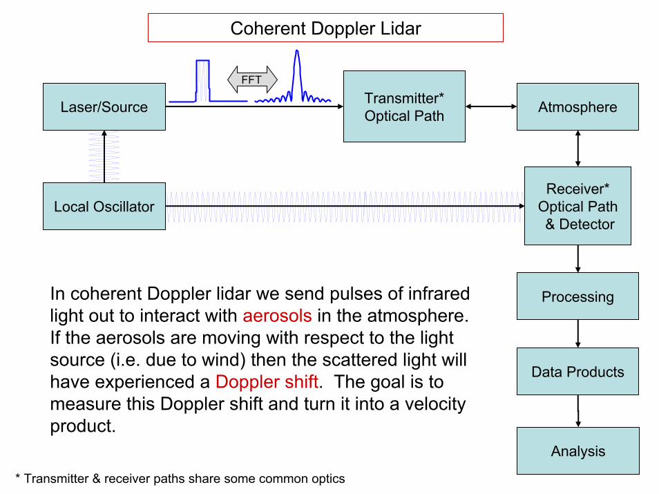
In coherent Doppler lidar we send pulses of infrared light out to interact with aerosols in the atmosphere. If the aerosols are moving with respect to the light source (i.e. due to wind) then the scattered light will have experienced a Doppler shift. The goal is to measure this Doppler shift and turn it into a velocity product.

* Transmitter & receiver paths share some common optics

Coherent Doppler Lidar

Laser/Source

Local Oscillator

Transmitter*Optical Path Atmosphere

Receiver*Optical Path& Detector

Processing

Data Products

Analysis

FFT

∫∞

⎟⎠⎞

⎜⎝⎛ −=

02

2 2, dRcRtP

RβTA

P Teff

r λ

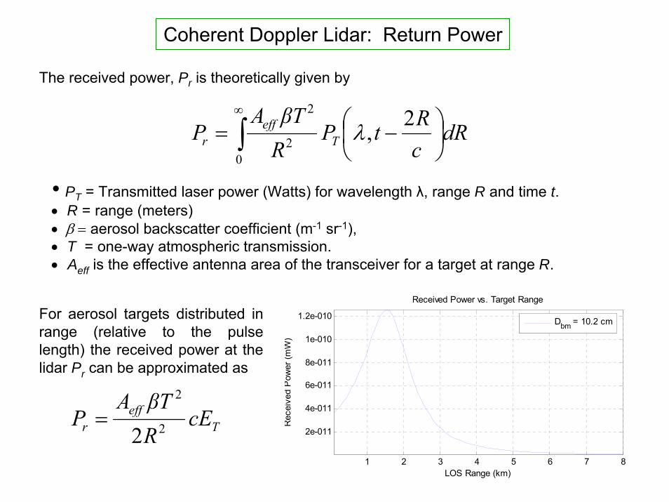
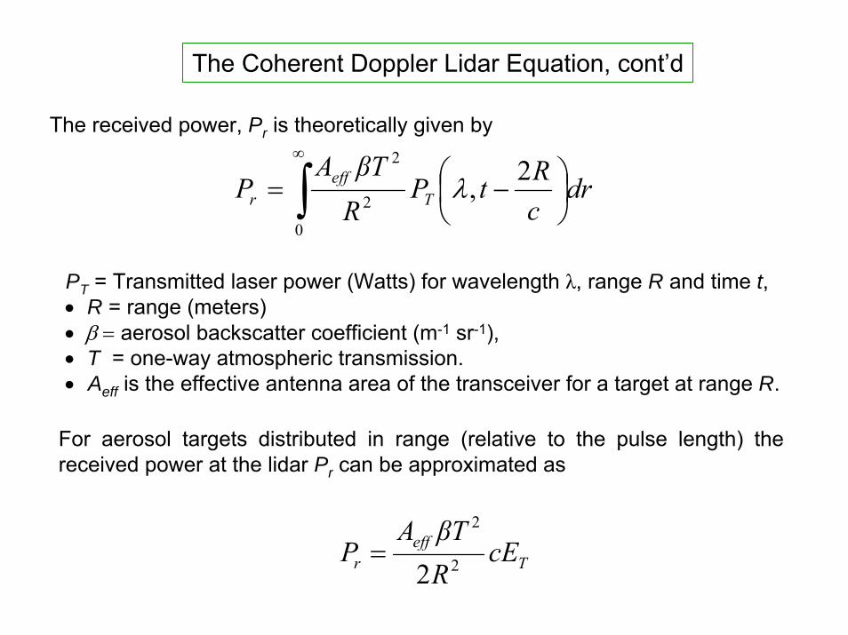
• PT = Transmitted laser power (Watts) for wavelength λ, range R and time t.• R = range (meters) • β = aerosol backscatter coefficient (m-1 sr-1), • T = one-way atmospheric transmission. • Aeff is the effective antenna area of the transceiver for a target at range R.

The received power, Pr is theoretically given by

Coherent Doppler Lidar: Return Power

Teff

r cERβTA

P 2

2

2=

For aerosol targets distributed in range (relative to the pulse length) the received power at the lidar Pr can be approximated as

1 2 3 4 5 6 7 8

2e-011

4e-011

6e-011

8e-011

1e-010

1.2e-010

Rec

eive

d P

ower

(mW

)

LOS Range (km)

Received Power vs. Target Range

Dbm = 10.2 cm

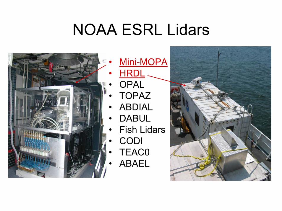
NOAA ESRL Lidars

• Mini-MOPA• HRDL• OPAL• TOPAZ• ABDIAL• DABUL• Fish Lidars• CODI• TEAC0• ABAEL

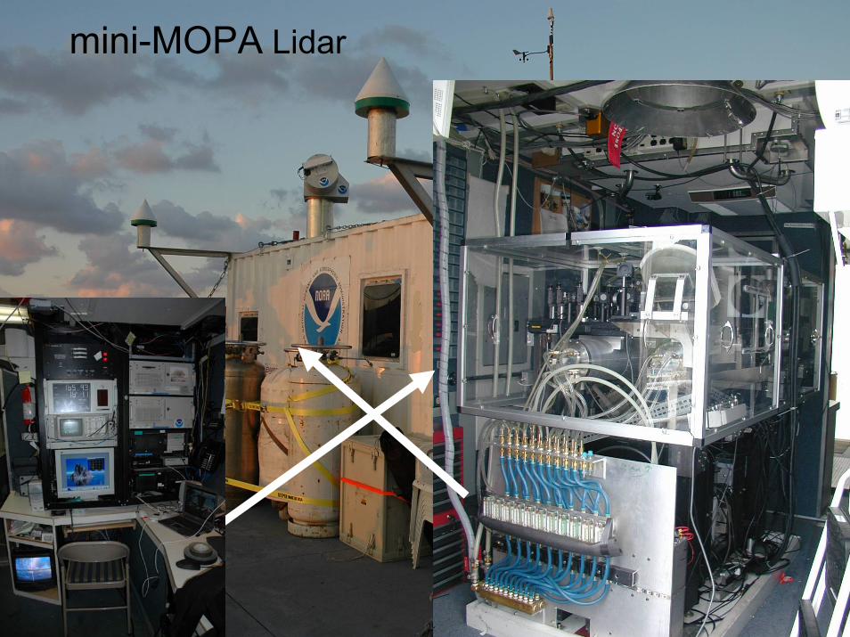
mini-MOPA Lidar

8 km

20 cm Ф

Lidar measurement volume:

• Diffraction limited divergence (60 µrad)• “Spotlight” beam can measure to within a

few meters of the surface (no side lobes)• 30-150 m measurement volume (range resolution) along the beam (Instrument dependent)

2ctΔ


Teff

r cERβTA

P 2

2

2=

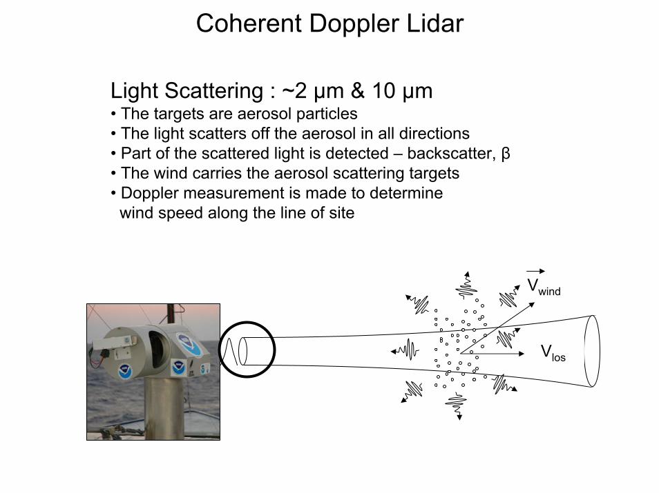
Light Scattering : ~2 μm & 10 μm• The targets are aerosol particles • The light scatters off the aerosol in all directions• Part of the scattered light is detected – backscatter, β• The wind carries the aerosol scattering targets• Doppler measurement is made to determinewind speed along the line of site

Vwind

Vlos


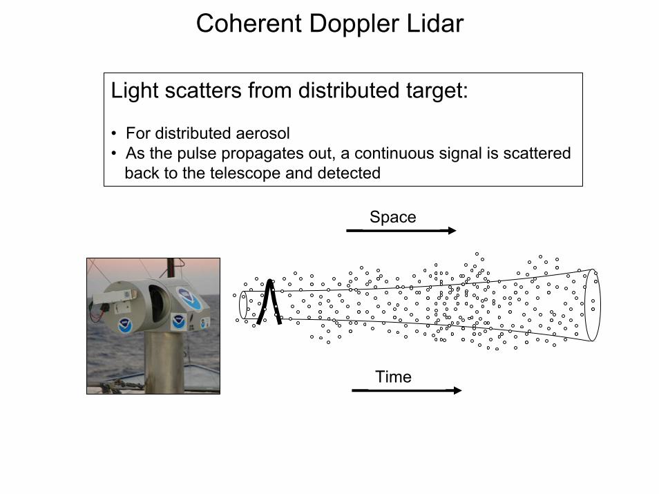
Light scatters from distributed target:

• For distributed aerosol• As the pulse propagates out, a continuous signal is scattered

back to the telescope and detected

Time

Space


• Coherent Detection• Laser • Local Oscillator + shift • Transmit/Receive paths• Atmosphere• Detection & Processing• Analysis and Data products• Field Work

Coherent Detection: The Doppler shift• The Doppler shift for illumination of wavelength λ is given by:

Where v is the velocity of the aerosol(s) (e.g. wind speed) and θv is the angle between the wind direction and the lidar line of sight (LOS)For a 15 m/s wind speed, the Doppler shift for 2μm light (fDopp = 1.5x1014 Hz) is 15 MHz.

• The returning illumination has a frequency of freturn = f +fDopp = 1.50000015x1014 Hz.

• Cutoff frequencies of our detectors are around GHz.• How can we detect such small Doppler shifts in frequencies

way above detection limit?

cf νν θυν

λθν cos2cos2

==Δ

Coherent DetectionDetecting Doppler Shifts

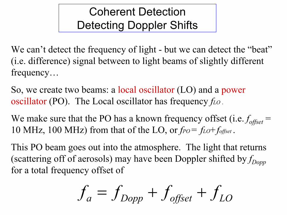
We can’t detect the frequency of light - but we can detect the “beat”(i.e. difference) signal between to light beams of slightly different frequency…

So, we create two beams: a local oscillator (LO) and a power oscillator (PO). The Local oscillator has frequency fLO .

We make sure that the PO has a known frequency offset (i.e. foffset = 10 MHz, 100 MHz) from that of the LO, or fPO = fLO+foffset .

This PO beam goes out into the atmosphere. The light that returns (scattering off of aerosols) may have been Doppler shifted by fDoppfor a total frequency offset of

LOoffsetDoppa ffff ++=

Coherent DetectionThe atmospheric return signal and the signal from the local oscillator are both incident on the detector.

Their electric fields add to create the total electric field incident on the detector:

( )( )

( ) ( )LOLOLOaaatot

LOLOLOLO

aaaa

tfjAtfjAEtfjAE

tfjAE

ϕπϕπϕπ

ϕπ

+++=+=

+=

2cos2cos2cos

2cos

Local Oscillator cos(2πf0+θ0)

Atmospheric return signal cos(2πfr+θr)

ReceiverDetector

( ) ( )( ) ( )

( ) ( )LOLOaaLOa

LOLOLOaaa

LOLOLOaaatot

tfjtfjAAtfjAtfjA

tfjAtfjAE

ϕπϕπϕπϕπ

ϕπϕπ

+++

+++=

+++=

2cos2cos22cos2cos

2cos2cos2222

22

( ) ( )( ) ( )( )( ) ( )( )LOaLOaLOa

LOaLOaLOa

LOLOLOaaatot

tffjAAtffjAA

tfjAtfjAE

ϕϕπϕϕπ

ϕπϕπ

−+−+++++

+++=

2cos22cos2

2cos2cos 22222

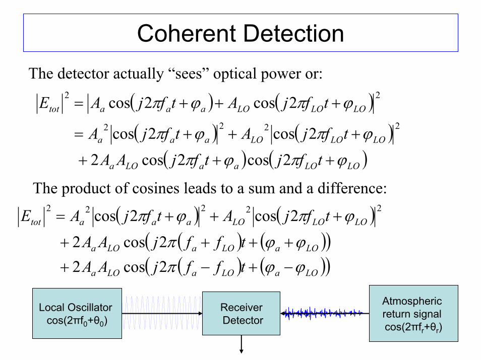
The product of cosines leads to a sum and a difference:

The detector actually “sees” optical power or:

Coherent Detection



ReceiverDetector

( ) ( )( )LOaLOaLOaLOatot tffjAAEEE ϕϕπ −+−++= 2cos222

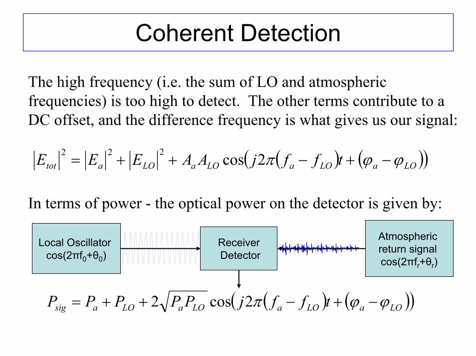
The high frequency (i.e. the sum of LO and atmospheric frequencies) is too high to detect. The other terms contribute to a DC offset, and the difference frequency is what gives us our signal:

In terms of power - the optical power on the detector is given by:

( ) ( )( )LOaLOaLOaLOasig tffjPPPPP ϕϕπ −+−++= 2cos2

Coherent Detection



ReceiverDetector

( ) ( )( )LOaLOaLOaLOasig

sig tffjiiiiheP

i ϕϕπυ

η−+−++=⎟⎟

⎠

⎞⎜⎜⎝

⎛= 2cos2

Remember ~ Mhz

We know foffset…so we can find the Doppler shift frequency.

offsetDoppLOa ffff +

The detector current is then given by:

=−

Coherent Detection



ReceiverDetector

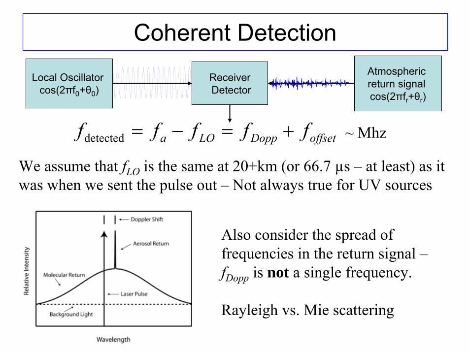
~ MhzoffsetDoppLOa fffff +=−=detected

Coherent Detection



ReceiverDetector

We assume that fLO is the same at 20+km (or 66.7 µs – at least) as it was when we sent the pulse out – Not always true for UV sources

Also consider the spread of frequencies in the return signal –fDopp is not a single frequency.

Rayleigh vs. Mie scattering

IR vs. UV in heterodyne detection

Property IR UV

Linewidth/Temporal Coherence

kHz 10s of km and longer (100 km)

Old: GHz metersNew: MHz 100s m

Rayleigh (very wide) & Mie

Detection noise Shot noise limited by LO

LO Shot noise + Rayleigh scattering

Aerosol sampling BW(SNR ∝1/BW)

2µm: 25 m/s needs 50 Mhz BW

355nm: 25 m/s needs ~300 Mhz

Refractive Turbulence Some effect (less for longer λ)

Stronger effect (less spatial coherence)

Scattering/BW Mie – pulse transform limited

λν2

=Δf

• Coherent Detection• Laser & pulses• Local Oscillator + shift • Transmit/Receive path • Atmosphere• Detection & Processing• Analysis and Data products• Field Work

Laser & PulsesLaser/Transmitter Requirements

• Narrow bandwidth (i.e. ~1 Mhz)• Q-switched or modulated• Low atmospheric absorption • High pulse repetition frequency (PRF)• 1-8 mJ per pulse• Eyesafe Tradeoffs between:

• short pulses• pulse bandwidth• PRF• average power

A fun intro to lasers….http://www.colorado.edu/physics/2000/lasers/index.html

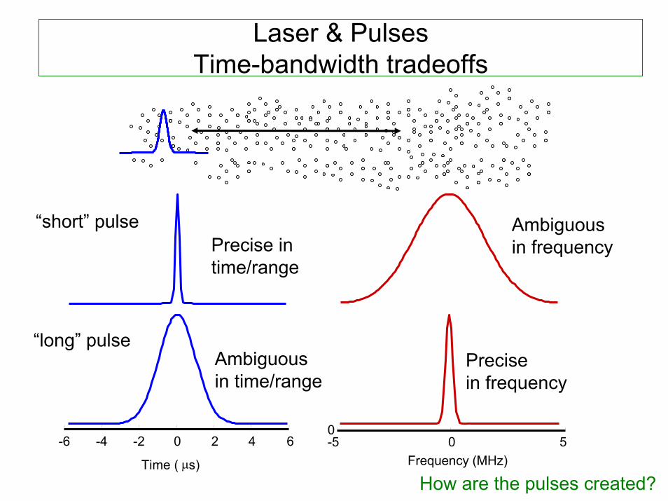
Laser & Pulses Time-bandwidth tradeoffs

-6 -4 -2 0 2 4 6

Time ( μs)

-5 0 50

Frequency (MHz)

Precisein frequency

Ambiguousin time/range

“long” pulse

Precise in time/range

Ambiguousin frequency

“short” pulse

How are the pulses created?

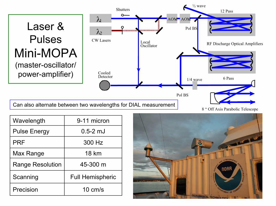
Laser & Pulses

Mini-MOPA(master-oscillator/ power-amplifier)

λ1

λ2

AOM1 AOM2

CW Lasers

Shutters

Pol BS

½ wave

Local Oscillator

12 Pass

RF Discharge Optical Amplifiers

6 Pass1/4 wave

8 “ Off Axis Parabolic Telescope

Pol BS

CooledDetector

Wavelength 9-11 micron

Max Range 18 km

Precision 10 cm/s

Pulse Energy 0.5-2 mJ

PRF 300 Hz

Range Resolution 45-300 m

Scanning Full Hemispheric

Can also alternate between two wavelengths for DIAL measurement

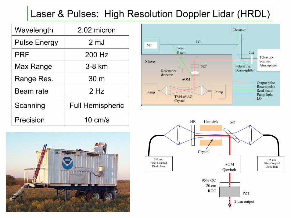
Wavelength 2.02 micron

Max Range 3-8 km

Scanning Full Hemispheric

Precision 10 cm/s

Pulse Energy 2 mJ

PRF 200 Hz

Range Res. 30 m

Beam rate 2 Hz

Detector

LO

Pump Pump TM:LuYAGCrystal

AOM

PZT

Seed Beam

Resonance detector

λ /4

PolarizingBeam-splitter

Output pulse Return pulse Seed beam Pump light LO

Telescope Scanner Atmosphere

Slave

MO

Laser & Pulses: High Resolution Doppler Lidar (HRDL)

785 nm Fiber Coupled

Diode Bars AOMQswitch

95% OC20 cm ROC

HR Heatsink

Crystal

M1

PZT

2 µm output

785 nm Fiber Coupled

Diode Bars

• Coherent Detection• Laser & pulses• Local Oscillator + shift• Transmit/Receive path • Atmosphere• Detection & Processing• Analysis and Data products• Field Work

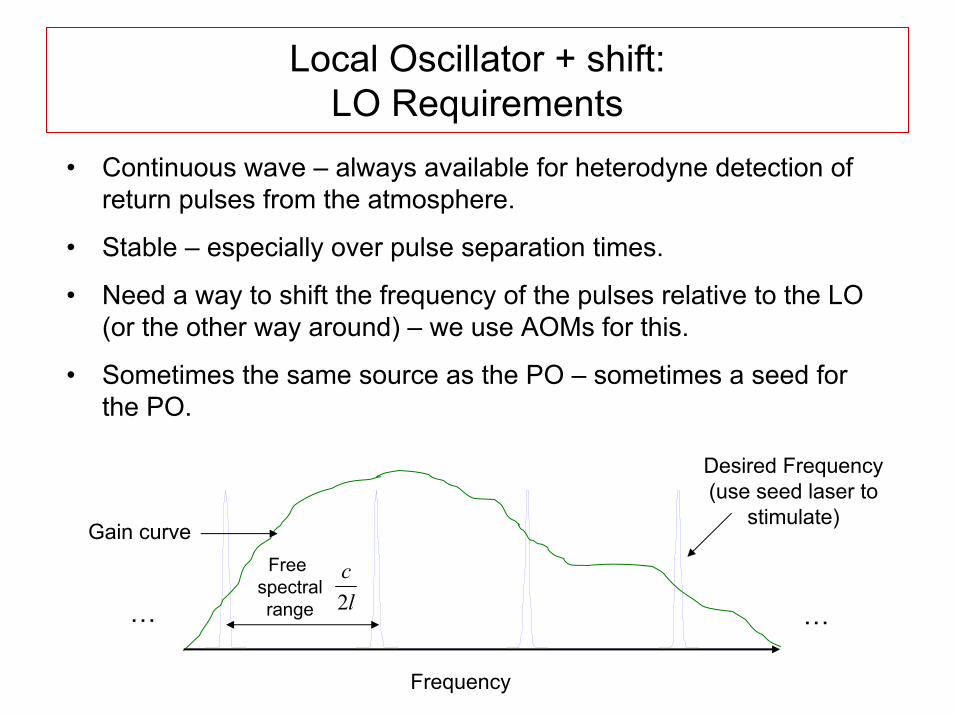
Local Oscillator + shift: LO Requirements

• Continuous wave – always available for heterodyne detection of return pulses from the atmosphere.

• Stable – especially over pulse separation times.

• Need a way to shift the frequency of the pulses relative to the LO (or the other way around) – we use AOMs for this.

• Sometimes the same source as the PO – sometimes a seed for the PO.

Free spectralrange

Gain curve

lc2

Desired Frequency(use seed laser to

stimulate)

Frequency

……

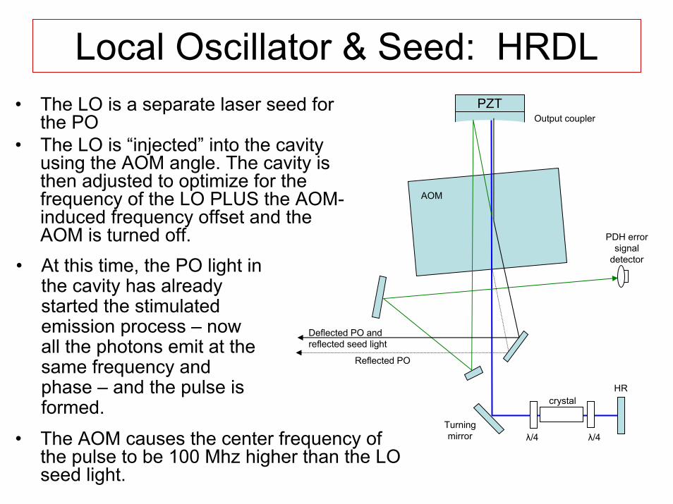
Local Oscillator & Seed: HRDL• The LO is a separate laser seed for

the PO• The LO is “injected” into the cavity

using the AOM angle. The cavity is then adjusted to optimize for the frequency of the LO PLUS the AOM-induced frequency offset and the AOM is turned off.

λ/4 λ/4

crystal

AOM

HR

Output coupler

Turning mirror

PDH error signal

detector

Deflected PO and reflected seed light

Reflected PO

• At this time, the PO light in the cavity has already started the stimulated emission process – now all the photons emit at the same frequency and phase – and the pulse is formed.

• The AOM causes the center frequency of the pulse to be 100 Mhz higher than the LO seed light.

PZT

18 pass RF discharge optical amplification

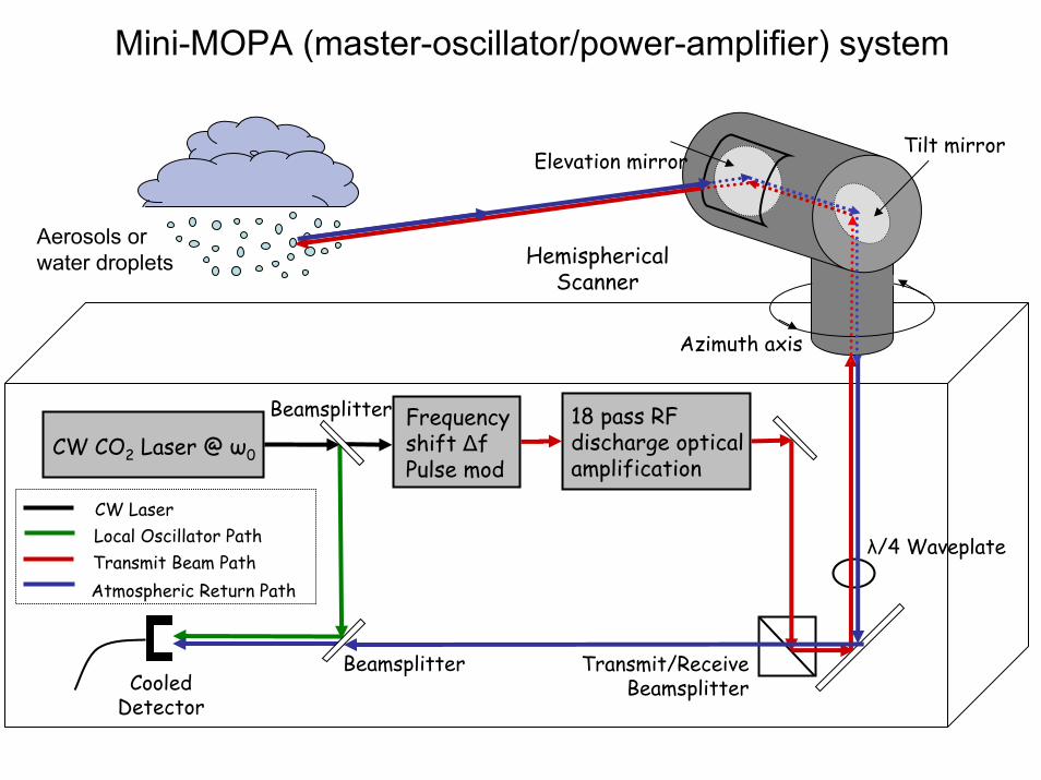
CooledDetector

CW CO2 Laser @ ω0

CW Laser

Frequency shift ΔfPulse mod

Transmit Beam Path

Hemispherical Scanner

Elevation mirrorTilt mirror

Azimuth axis

Aerosols or water droplets

Transmit/ReceiveBeamsplitter

Atmospheric Return Path

Local Oscillator Path

Beamsplitter

Beamsplitter

Mini-MOPA (master-oscillator/power-amplifier) system

λ/4 Waveplate

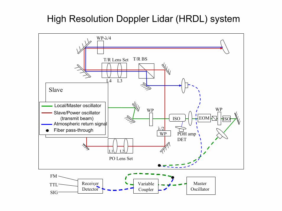
FM

TTLSIG

Slave

Master Oscillator

Variable Coupler

ISO ISOEOM

Receiver Detector

PDH ampDET

T/R BST/R Lens Set

WP

WP-λ/4

WPλ/2

L3L4

PO Lens SetL1 L2

WPLocal/Master oscillatorSlave/Power oscillator

(transmit beam)Atmospheric return signalFiber pass-through

High Resolution Doppler Lidar (HRDL) system

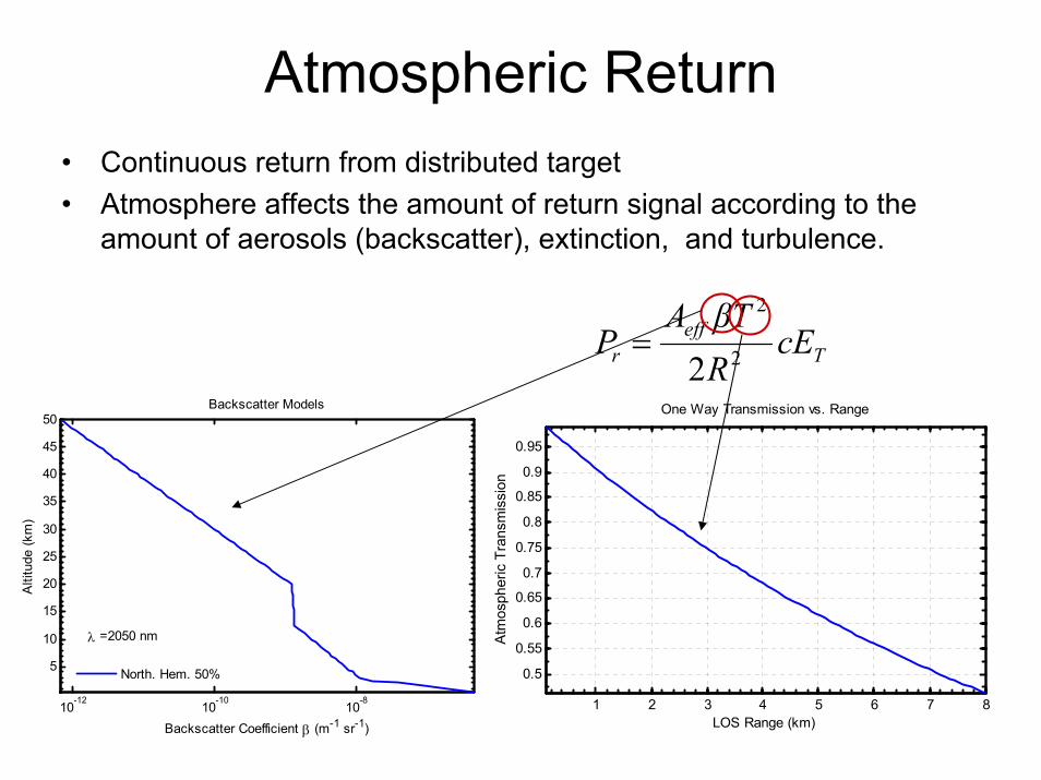
Atmospheric Return• Continuous return from distributed target• Atmosphere affects the amount of return signal according to the

amount of aerosols (backscatter), extinction, and turbulence.

10-12 10-10 10-8

5

10

15

20

25

30

35

40

45

50

Backscatter Coefficient β (m-1 sr-1)

Alti

tude

(km

)

Backscatter Models

λ =2050 nm

North. Hem. 50%

Teff

r cERβTA

P 2

2

2=

1 2 3 4 5 6 7 8

0.5

0.55

0.6

0.65

0.7

0.75

0.8

0.85

0.9

0.95

Tran

smis

sion

LOS Range (km)

One Way Transmission vs. Range

Atm

osph

eric

Tra

nsm

issi

on

BhP

i

iCNR r

N

het

νη

==2

2

The carrier-to-noise ratio (CNR) is found using the following equation:

• where η is an efficiency factor (less than or equal to unity) describing the noise sources in the photo-detector signal as well as optical efficiencies, • h is Plank’s constant (6.626x10-34 Joule-sec)• ν is the optical frequency (Hz.) • B is the receiver bandwidth determined by the receiver electronics.

- In HRDL’s case, B is 50 MHz. - In MOPA’s case, B is 10 MHz• Rule of thumb: We need about one coherent photon per inverse

BW to get 0 dB CNR – i.e. Coherent Doppler Lidar is quite sensitive.

The Coherent Doppler Lidar Equation

∫∞

⎟⎠⎞

⎜⎝⎛ −=

0

2

2 2, drcRtP

RβTA

P Teff

r λ

The received power, Pr is theoretically given by

PT = Transmitted laser power (Watts) for wavelength λ, range R and time t, • R = range (meters) • β = aerosol backscatter coefficient (m-1 sr-1), • T = one-way atmospheric transmission. • Aeff is the effective antenna area of the transceiver for a target at range R.

The Coherent Doppler Lidar Equation, cont’d

Teff

r cERβTA

P 2

2

2=

For aerosol targets distributed in range (relative to the pulse length) the received power at the lidar Pr can be approximated as

⎟⎟⎠

⎞⎜⎜⎝

⎛+=

turbTReff AAA1121

2

2

2

2

118

21⎟⎠⎞

⎜⎝⎛ −+=

RFD

DATR λπ

π

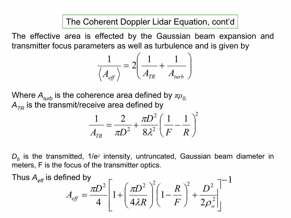
Where Aturb is the coherence area defined by πρ0.ATR is the transmit/receive area defined by

The effective area is effected by the Gaussian beam expansion and transmitter focus parameters as well as turbulence and is given by

Db is the transmitted, 1/e2 intensity, untruncated, Gaussian beam diameter in meters, F is the focus of the transmitter optics.


1

21

41

4 2

22222−

⎥⎥⎦

⎤

⎢⎢⎣

⎡+⎟

⎠⎞

⎜⎝⎛ −⎟⎟

⎠

⎞⎜⎜⎝

⎛+=

oeff

DFR

RDDA

ρλππ

Thus Aeff is defined by

53

22

8345.1

−

⎥⎦⎤

⎢⎣⎡= RCk noρ

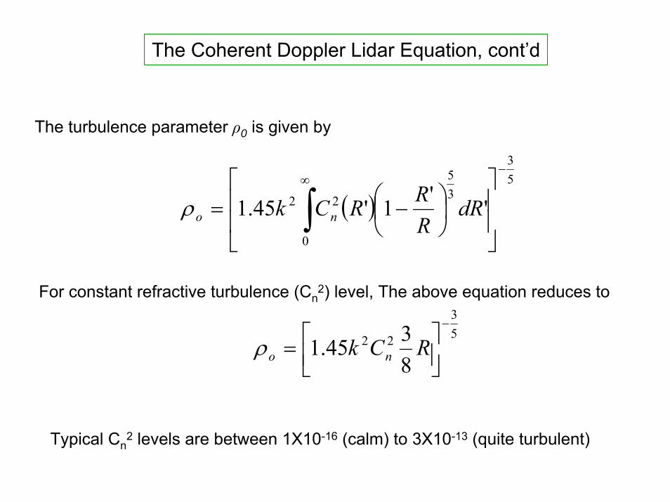
For constant refractive turbulence (Cn2) level, The above equation reduces to

The turbulence parameter ρ0 is given by

( )53

0

35

22 ''1'45.1

−∞

⎥⎥

⎦

⎤

⎢⎢

⎣

⎡⎟⎠⎞

⎜⎝⎛ −= ∫ dR

RRRCk noρ

Typical Cn2 levels are between 1X10-16 (calm) to 3X10-13 (quite turbulent)


1

21

41

42)( 2

22222

2

2−

⎥⎥⎦

⎤

⎢⎢⎣

⎡+⎟

⎠⎞

⎜⎝⎛ −⎟⎟

⎠

⎞⎜⎜⎝

⎛+=

o

T DFR

RDD

RBhcEβTRCNR

ρλππ

νη

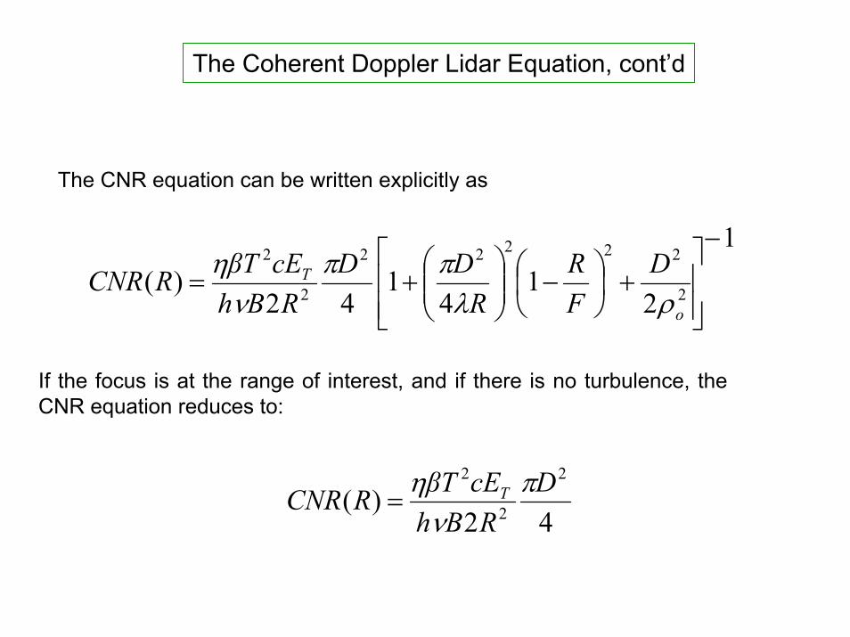
The CNR equation can be written explicitly as

42)(

2

2

2 DRBh

cEβTRCNR T πν

η=

If the focus is at the range of interest, and if there is no turbulence, the CNR equation reduces to:



Next lecture…

optical remote sensing with coherent doppler...

Documents