operator theory - spectra and functional...

Operator Theory - Spectra andFunctional Calculi

Alan McIntoshLecture notes taken by Lashi Bandara

February 18, 2010

Contents

Introduction 1

Overview and Motivation 2

1 Preliminaries 5

1.1 Banach Spaces . . . . . . . . . . . . . . . . . . . . . . . . . . . . . . . . . . 5

1.2 Direct Sums of Banach Spaces . . . . . . . . . . . . . . . . . . . . . . . . . 7

1.3 Integration of Banach Valued Functions . . . . . . . . . . . . . . . . . . . . 8

1.4 Banach Algebras . . . . . . . . . . . . . . . . . . . . . . . . . . . . . . . . . 9

1.5 Holomorphic Banach valued functions . . . . . . . . . . . . . . . . . . . . . 11

2 Functional Calculus of bounded operators 15

2.1 Spectral Theory of bounded operators . . . . . . . . . . . . . . . . . . . . . 15

2.2 Functions of operators . . . . . . . . . . . . . . . . . . . . . . . . . . . . . . 17

2.3 Holomorphic functional calculus . . . . . . . . . . . . . . . . . . . . . . . . . 19

2.4 Spectral decomposition . . . . . . . . . . . . . . . . . . . . . . . . . . . . . . 23

2.5 Exponentials and Fractional powers . . . . . . . . . . . . . . . . . . . . . . 24

2.6 Spectral Projections . . . . . . . . . . . . . . . . . . . . . . . . . . . . . . . 26

2.7 Duality . . . . . . . . . . . . . . . . . . . . . . . . . . . . . . . . . . . . . . 29

3 Unbounded Operators 33

i

3.1 Closed Operators . . . . . . . . . . . . . . . . . . . . . . . . . . . . . . . . . 33

3.2 Functional calculus for closed operators . . . . . . . . . . . . . . . . . . . . 36

4 Sectorial Operators 40

4.1 The Ψ functional calculus . . . . . . . . . . . . . . . . . . . . . . . . . . . . 40

4.2 Semigroup Theory . . . . . . . . . . . . . . . . . . . . . . . . . . . . . . . . 47

4.3 H∞ Functional Calculus . . . . . . . . . . . . . . . . . . . . . . . . . . . . . 49

5 Operators on Hilbert Spaces 50

5.1 The numerical range . . . . . . . . . . . . . . . . . . . . . . . . . . . . . . . 51

5.2 Functional calculus and numerical range . . . . . . . . . . . . . . . . . . . . 54

5.3 Accretive operators . . . . . . . . . . . . . . . . . . . . . . . . . . . . . . . . 55

5.4 Closed operators . . . . . . . . . . . . . . . . . . . . . . . . . . . . . . . . . 57

5.5 Fractional powers . . . . . . . . . . . . . . . . . . . . . . . . . . . . . . . . . 61

5.6 Bisectorial operators . . . . . . . . . . . . . . . . . . . . . . . . . . . . . . . 62

5.7 Bounded H∞ functional calculus of bisectorial operators . . . . . . . . . . . 64

Notation 71

ii

Introduction

The principal theme of this course concerns definitions and bounds on functions f(T ) oflinear operators in Banach spaces X , in particular in Hilbert spaces. Ideally the boundswould be of the form f(T ) f∞, or better still f(T ) ≤ f∞. The latter hap-pens when T is a self-adjoint operator in a Hilbert space and f is a Borel measurablefunction on the real line. For example if X = CN and T is represented by the matrix

T =

λ1 0λ2

. . .0 λN

, then f(T ) =

f(λ1) 0f(λ2)

. . .0 f(λN )

and so f(T ) ≤ max |f(λj)| ≤ f∞. However such estimates cannot always be obtained,

as is indicated by the example Tn =

1n 1

0 1n

and f(ζ) =

√ζ, because f(Tn) = Tn

1/2 =

1√n

√n

2

0 1√n

blows up as n →∞.

It is assumed that the reader has a basic knowledge of topology, metric spaces, Banach andHilbert spaces, and measure theory. Suitable references for this material are the books Realand Complex Analysis by W. Rudin, Real Analysis by H.L. Royden [Rud87], Introduction toTopology and Modern Analysis by G.F. Simmons [Sim83], Functional Analysis by F. Rieszand B. Sz.-Nagy [RSN90], and Linear Operators, Part I, General Theory by N. Dunfordand J.T. Schwartz [DS88]. Later, we may also expect some knowledge of Fourier theoryand partial differential equations.

Useful books include: Tosio Kato, Perturbation theory for linear operators [Kat76]; PaulHalmos, Introduction to Hilbert space [Hal98]; Edgar Lorch, Spectral theory [Lor62]; MichaelReed and Barry Simon, Methods of modern mathematical physics. I. Functional analysis[RS72].

Parts of these lectures are based on the lecture notes Operator theory and harmonic analy-sis by David Albrecht, Xuan Duong and Alan McIntosh [ADM96], which are in turn basedon notes taken, edited, typed and refined by Ian Doust and Elizabeth Mansfield, whosewilling assistance is gratefully acknowledged.

1

Overview and Motivation

Let T ∈ L (X). We construct a functional calculus which is an algebra homomorphismΦT : H(Ω) −→ L (X). Here, σ (T ) ⊂ Ω, and Ω is open in C. The functional calculussatisfies the following properties:

f → f(T )1 → I

id → T

In addition, if the spectrum of T breaks up into two disjoint compact components σ+(T ), σ−(T ),we want χ+ → P+ := χ+(T ) and χ− → P− := χ−(T ). In this case, we can writeX = X+ ⊕ X−, where X± = R(P±). This is the background setting. Naturally, we wantvarious generalisations of this.

The first is to consider the situation when we have some λ ∈ σ (T ), and σ (T ) \ λ ⊂ Ω.We want to find a suitable class of operators T to define f(T ) ∈ L (X) when f ∈ H(Ω)such that f(T ) ≤ C f ∞.

In analogy to the earlier situation, now suppose that σ (T )\λ breaks up into two compactsets σ+(T ), σ−(T ). Then, if P± are bounded, then as before, we have X = X+ ⊕ X−.

Another natural generalisation is to relax the condition that T ∈ L (X). For closedoperators, we find σ (T ) is a compact subset of the extended complex plane C∞. We wantto find suitable unbounded T for each of the following situations:

1. σ (T ) ⊂ Ω

2. σ (T ) \ ∞ ⊂ Ω

3. σ (T ) \ 0,∞ ⊂ Ω.

4. σ (T ) \ 0,∞ breaks into two components, each contained in a sector on the leftand right half planes of C.

The last is a particularly important case, as illustrated by the following example.

Let X = L2(R), and let D = T = 1

iddx . This is a unbounded, self adjoint operator

σ (D) = R∪∞. As before, we can write σ−(T ), σ+(T ) respectively for the left and right

2

half planes and:

P± = χ±(D) = χ± ∞ = 1

Let,

sgn(λ) =

−1 Re λ > 00 Re λ = 0+1 Re λ < 0

Observe that (sgnλ)√

λ2 = λ, and sgn(λ)λ =√

λ2. Also, sgn(D) = χ+(D) − χ−(D) and sgn(D) = 1. Here, H := sgn(D) is the Hilbert transform, and

√D2 = HD, H

√D2 = D.

We can also consider replacing L2(R) by L

p(R). In fact, we can find that H = sgn(D) =χ+(D)+χ−(D) is bounded. The self adjoint theory no longer applies to access such resultsand instead, dyadic decompositions near 0 and ∞ are needed. These are the beginningsof Harmonic Analysis.

We also want to look for n dimensional analogues. The setting is as follows. Let H =L

2(Rn)⊕L2(Rn

,Cn). Here, we have∇ : L2(Rn) −→ L

2(Rn,Cn) and div : L

2(Rn,Cn) −→

L2(Rn). In fact,

−∇f, u =

j

∂f

∂xjuj =

f

∂uj

∂xj= f, div u

So, each operator is dual to the negative of the other.

Let A = (Ajk)nj,k=1 where Ajk ∈ L

∞(Rn). Also we assume the following ellipticity condi-tion: ζ ∈ Cn, and for almost all x ∈ Rn,

Re

Ajkζjζk ≥ |x||ζ|2

Define the operator T : H→ H:

T =

0 divA

−∇ 0

We find that σ (T ) ⊂ 0,∞∪Soω+∪S

oω− where S

oω+ = ζ ∈ C \ 0 : | arg ζ| < ω, S

oω− =

−Soω+ and we can formulate a generalised Hilbert transform as H = sgn(T ). A recent

deep theorem then gives: T has a bounded functional calculus and in particular, sgn(T )is bounded.

As a consequence, we have:√

T 2 = sgn(T )T

T = sgn(T )√

T 2

and√

T 2u

Tu .

3

Furthermore, observe that:

√

T 2 =√

−div A∇ 00

√−∇div A

√−div A∇ 0

0√−∇div A

f

u

0 divA

−∇ 0

f

u

Setting u = 0 we find:√−div A∇

∇f

This is the Kato Square Root problem [AHL+02]. See [AMK] and [AM] for further details.

4

Chapter 1

Preliminaries

1.1 Banach Spaces

We work in a Banach Space. This is a normed linear space that is complete. More formally,

Definition 1.1.1 (Banach Space (over C)). We say that X is a Banach space if:

(i) X is a linear space over C.

(ii) There is a norm · : X → R. That is:

(a) u = 0 =⇒ u = 0(b) u + v ≤ u + v (Triangle Inequality)(c) αu = |α| u

For all α ∈ C and u, v ∈ X .

(iii) X is complete in the metric ρ(u, v) = u− v , or in other words every Cauchysequence (xn) in X converges to some x ∈ X . That is, if ρ(xn, xm) → 0, there existsan x ∈ X such that ρ(xn, x) → 0.

Exercise 1.1.2. Show that C × C × X × X → X given by (α,β, u, v) → αu + βv iscontinuous.

Since a Banach space has a vector space structure, we can talk about infinite series in thesame way we treat infinite series of complex numbers.

Definition 1.1.3 (Infinite Series). Let (xn)∞i=1 be a sequence in X . We define partialsums Sn :=

ni=1 xn. If there is an S ∈ X such that limn→∞ Sn = S, then we write:

S =∞

j=1

xj

and we say that the infinite series∞

i=1 xn converges.

5

Definition 1.1.4 (Absolutely Convergent). We say that a series∞

n=1 xn is absolutelyconvergent if

∞n=1 xn is convergent.

Proposition 1.1.5. Every absolutely convergent series is convergent.

Proof. We show that the partial sums Sn are Cauchy. Let n > m. Then by the triangleinequality,

Sn − Sm =

n

j=m+1

xj

≤

n

j=m+1

xj

The right hand side tends to 0 as m, n → ∞ sincem

j=1 xj is convergent and conse-quently Cauchy.

Example 1.1.6. (i) Cn with

u p =

(|uj |

p)1p 1 ≤ p < ∞

sup |uj | = max |uj | p = ∞

These norms are all equivalent since Cn is finite dimensional.

(ii) p =

u = (uj)∞j=1 : u p < ∞

, with u p the same as above. .

(iii) Lp(Ω) =

f : Ω → R : f p < ∞

, where Ω is a σ-finite measure space, where:

f p =

Ω |f |

p 1

p 1 ≤ p < ∞

ess sup|f | p = ∞

(iv) Cb(M) = f : M → C : f ∞ < ∞, where f ∞ = supx∈M |f(x)|.

(v) H∞(Ω) = f : Ω → C bounded and holomorphic, where Ω ⊂ C open and again

equipped with · ∞.

Note that: H∞(Ω) ⊂ Cb(Ω) ⊂ L

∞(Ω).

(vi) L (X ,Y) is the space of bounded linear maps from X to Y where X is normed andY is a Banach Space. The latter condition is necessary and sufficient for L (X ,Y) tobe a Banach space. The norm here is the operator norm:

T = supx =0

Tx Yx X

= supx X=1

Tx Y

(vii) L (X ) = L (X ,X ).

6

1.2 Direct Sums of Banach Spaces

Given two Banach spaces, we can define the notion of a direct sum.

Definition 1.2.1 (Direct sum of Banach spaces). Let X1,X2 be Banach Spaces. Define:

X = X1 ⊕ X2 = (u1, u2) : ui ∈ Xi

u = (u1, u2) = u1 X1+ u2 X2

Operators on the direct sum can be defined as follows.

Definition 1.2.2 (Direct sum of operators). Let Tj ∈ L (Xj), and X = X1 ⊕ X2. DefineT ∈ L (X ):

Tu = (T1u1, T2u2)

We also write:

Tu =

T1 00 T2

u1

u2

Proposition 1.2.3.

σ (T ) = σ (T1) ∪ σ (T2)f(T ) = f(T1)⊕ f(T2)

Proof. Exercise.

By induction, we can extend this to X =n

j=1Xj .

Another notion of direct sums is required to write a Banach space as a sum of subsets.

Definition 1.2.4 (Banach space as a direct sum of subsets). Let Y,Z ⊂ X . Then writingX = Y ⊕ Z means that:

(i) Y,Z are linear subspaces

(ii) Y ∩ Z = 0.

(iii) For all x ∈ X , there exists y ∈ Y, z ∈ Z and a C > 0 such that x = y + z with

y + z ≤ C x

Remark 1.2.5. It is worth noting that we have no concept of orthogonality here.

The following consequences are immediate.

Proposition 1.2.6. (i) x y + z

(ii) The decomposition is unique

7

(iii) Y,Z are closed

Definition 1.2.7 (Projection). We say P ∈ L (X ), is a projection if P2 = P .

Proposition 1.2.8. Given X = Y ⊕Z there exist a projection P ∈ L (X ) with R(P ) = Y

and N(P ) = R(I − P ) = Z. Conversely given a projection P ∈ L (X) we can decomposeX = N(P )⊕ R(P ).

This extends to the situation X =n

j=1Xj . We get projections Pj ∈ L (X) with R(Pi) =Xi, I =

nj=1 Pj , P

2j = Pj and PjPk = 0 when j = k.

1.3 Integration of Banach Valued Functions

As in the case of R, we can define various notions of integration. The following will besufficient for our purposes.

Definition 1.3.1 (Definite (Riemann) integral of Banach valued functions). Let f :[a, b] → X be a continuous function. Define xj = j(b−a)

n and:

b

af(τ)dτ = lim

n→∞

n−1

j=1

(xj+1 − xj)f(xj) = limn→∞

n−1

j=1

b− a

nf

j(b− a)

n

Remark 1.3.2. The limit exists since f : [a, b] → R is continuous and so any suchpartial sum is absolutely convergent.

Remark 1.3.3. It is also possible to easily generalise this to piecewise continuous functionsas in the R case.

Proposition 1.3.4.

b

af(τ)dτ

≤ b

a f(τ) dτ

Just as in the real variable case, we also consider indefinite integrals.

Definition 1.3.5 (Indefinite Integral of Banach valued functions). Let f : (a, b] → X becontinuous, where −∞ ≤ a < b < ∞. Define:

b

af(τ)dτ = lim

a→a

b

af(τ)dτ

whenever the limit exists.

Proposition 1.3.6. If f is absolutely integrable, then f is integrable and

b

af(τ)dτ

≤ b

a f(τ) dτ

Proof. Exercise.

8

Similarly, it is useful to define the contour integral when the domain of a function is C.

Definition 1.3.7 (Contour integral of a Banach valued function). Let f : Ω → X be acontinuous function, and let γ : [a, b] → Ω be a continuous curve. Define xj = j(b−a)

n and:

γf(ζ)dζ = lim

n→∞

n−1

j=1

[γ(xj+1)− γ(xj)] f(xj)

Remark 1.3.8. Again, this can be easily generalised to piecewise continuous curves.

Definition 1.3.9 (Piecewise Ck curve). If γ : [0, n + 1] → C and γ =

nj=1 γj , where

each γj ∈ Ck([j, j + 1],C), then we say that γ is a piecewise C

k curve.

Definition 1.3.10 (Closed contour). Let γ : [0, 1] → C be a curve such that γ(0) = γ(1).Then we say that γ is a closed contour.

1.4 Banach Algebras

Informally, a Banach algebra is a Banach space which has multiplication. It has a richerstructure that will be useful to us.

Definition 1.4.1 (Banach Algebra). Let X be a Banach space and further suppose thatthere is a map · : X × X → X , (u, v) → uv satisfying

(i) u(vw) = (uv)w (Associative)

(ii) u(v + w) = uv + uw (Left distributive)

(iii) (v + w)u = vu + wu (Right distributive)

(iv) λ(uv) = (λu)v = u(λv)

(v) uv ≤ u v

for all u, v ∈ X and λ ∈ C.

Proposition 1.4.2. (i) The map X × X → X which sends (u, v) → uv is continuous.

(ii)u

k ≤ u

k.

Proof. Exercise.

Definition 1.4.3 (Banach Algebra with identity). If X is a Banach algebra and thereexists an element e ∈ X such that eu = ue = u for all u ∈ X , then we call this elementan identity (or unit) and the algebra a Banach algebra with identity or a Unital Banachalgebra. Often, we denote the identity simply with 1 or I.

Definition 1.4.4 (Invertible). Let X be a Banach algebra with identity. We say that anelement u ∈ X is invertible if there exists u

−1 ∈ X such that uu−1 = 1 = u

−1u. We call

u−1 the inverse of u.

9

Many of the spaces that we have seen so far are Banach algebras.

Example 1.4.5. (i) l∞

, L∞(Ω), Cb(M),H∞(Ω),L (X) are all Banach algebras with iden-

tity

(ii) Let C0(X ) = f ∈ Cb(X ) : f(x) → 0 as x → ∞. This is a Banach algebra but itdoes not have an identity, since f ≡ 1 does not decay at ∞.

For a Banach algebra with identity, we can define polynomials in the algebra.

Definition 1.4.6. Let X be a Banach algebra with identity. For each polynomial p(ζ) =nj=0 αjζ

j , αj ∈ C and u ∈ X , define:

p(u) =n

j=0

αnuj, αn ∈ C

Remark 1.4.7. Note that:

n

i=0

αnuk

≤n

i=0

|αn|

uk

Recall that the following formal expression has a radius of convergence R ∈ [0,∞] forαk ∈ C, z ∈ C:

f(z) =∞

n=0

αkzk

This series diverges for |z| > R and converges absolutely when |z| < R.

Definition 1.4.8 (Power Series). Suppose f(z) =∞

n=0 αkzk is a power series with a

radius of convergence R ∈ [0,∞]. Let u ∈ X with u < R. Then, we define:

f(u) :=∞

n=0

αkuk∈ X

We can think of the map u → f(u) as a functional calculus of u as it is a Banach algebrahomomorphism which sends a complex valued function to a Banach valued function.

In a Banach algebra with identity X , we are also interested in invertibility and stability.

Proposition 1.4.9. Suppose that u ∈ X and that u < 1. Then (1 − u) is invertibleand (1− u)−1

≤ 11− u

.

indeed, (1− u)−1 =∞

k=0 uk.

Proof. As u < 1 and uk ≤ uk, then∞

k=0

uk =

11− u

.

10

Thus∞

k=0 uk = w for some w ∈ X . Now

(1− u)w = limn→∞

(1− u)n

k=0

uk (since (1− u) is a continuous mapping)

= limn→∞

(1− un+1)

= 1 .

The proof that w(1− u) = 1 is similar.

Theorem 1.4.10. Suppose that u ∈ X is invertible and that w ∈ X satisfies

w < u−1−1

.

Then u− w is invertible in X and

(u− w)−1 ≤ u−1

1− wu−1.

Proof. Write u−w = (1−wu−1)u. Now wu

−1 ≤ wu−1 < 1, and so (1−wu−1) is

invertible with(1− wu

−1)−1 ≤

11− wu−1

.

1t follows that u− w is invertible with

(u− w)−1 = u−1(1− wu

−1)−1∈ X .

Corollary 1.4.11. The set of invertible elements of X is an open set.

1.5 Holomorphic Banach valued functions

We begin by defining a notion of holomorphic for Banach valued functions.

Definition 1.5.1 (Holormorphic). Suppose that Ω is an open subset of C and that f :Ω → X . Then we say that f is holomorphic (or differentiable) if for every z ∈ Ω thereexists f

(z) ∈ X such that

f(z + h)− f(z)h

− f(z)

→ 0 as h → 0 ;

The set of all such functions are denoted by H(Ω,X ), and we write H(Ω) := H(Ω,C).

The reason we call such functions holomorphic is justified in the following theorem.

Theorem 1.5.2. Suppose that Ω is an open subset of C and that f : Ω → X . Then thefollowing are equivalent:

11

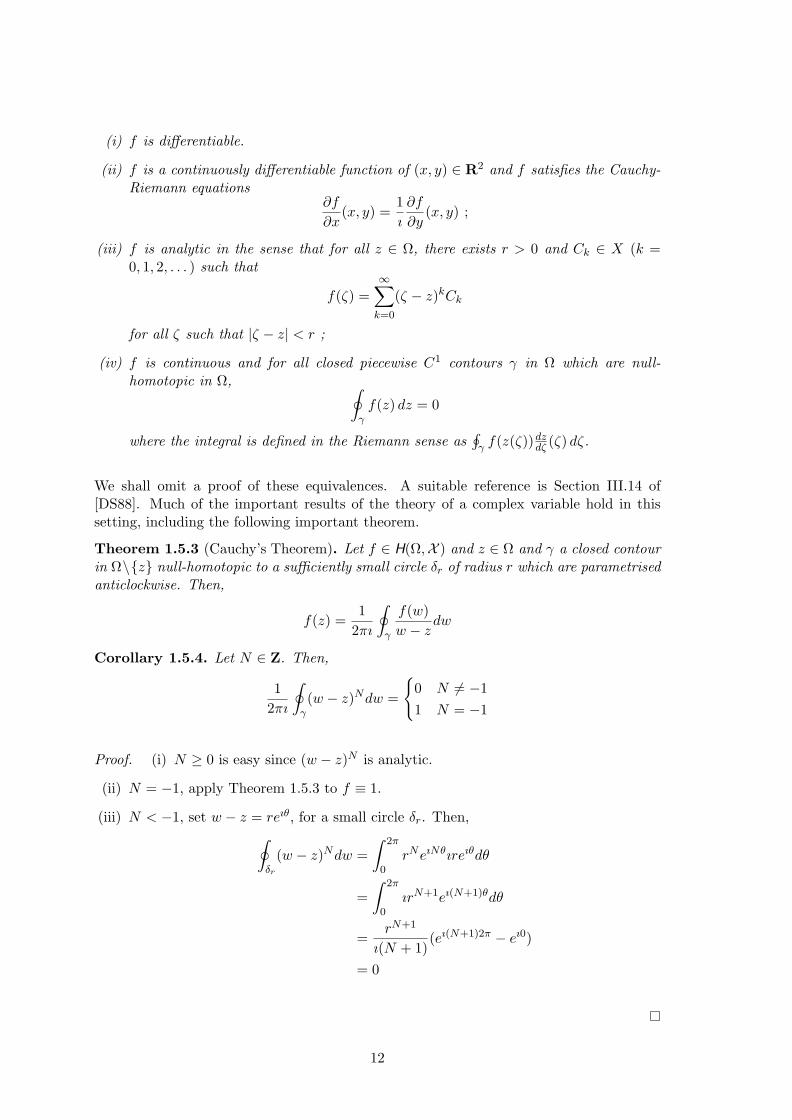
(i) f is differentiable.

(ii) f is a continuously differentiable function of (x, y) ∈ R2 and f satisfies the Cauchy-Riemann equations

∂f

∂x(x, y) =

1ı

∂f

∂y(x, y) ;

(iii) f is analytic in the sense that for all z ∈ Ω, there exists r > 0 and Ck ∈ X (k =0, 1, 2, . . . ) such that

f(ζ) =∞

k=0

(ζ − z)kCk

for all ζ such that |ζ − z| < r ;

(iv) f is continuous and for all closed piecewise C1 contours γ in Ω which are null-

homotopic in Ω,

γf(z) dz = 0

where the integral is defined in the Riemann sense asγ f(z(ζ))dz

dζ (ζ) dζ.

We shall omit a proof of these equivalences. A suitable reference is Section III.14 of[DS88]. Much of the important results of the theory of a complex variable hold in thissetting, including the following important theorem.

Theorem 1.5.3 (Cauchy’s Theorem). Let f ∈ H(Ω,X ) and z ∈ Ω and γ a closed contourin Ω\z null-homotopic to a sufficiently small circle δr of radius r which are parametrisedanticlockwise. Then,

f(z) =1

2πı

γ

f(w)w − z

dw

Corollary 1.5.4. Let N ∈ Z. Then,

12πı

γ(w − z)N

dw =

0 N = −11 N = −1

Proof. (i) N ≥ 0 is easy since (w − z)N is analytic.

(ii) N = −1, apply Theorem 1.5.3 to f ≡ 1.

(iii) N < −1, set w − z = reıθ, for a small circle δr. Then,

δr

(w − z)Ndw =

2π

0rN

eıNθ

ıreıθ

dθ

= 2π

0ır

N+1eı(N+1)θ

dθ

=rN+1

ı(N + 1)(eı(N+1)2π

− eı0)

= 0

12

Theorem 1.5.5 (Liouville’s Theorem). Suppose that f : C → X is holomorphic, andbounded in the sense that there exists M > 0 such that f(z) < M for all z ∈ C. Thenf is constant.

Definition 1.5.6 (Bounded holomorphic functions). We denote the space of boundedholomorphic functions from Ω into X by H

∞(Ω,X ).

Proposition 1.5.7. H∞(Ω,X ) is a Banach space with respect to the · ∞ norm.

Proof. Let fn ⊂ H∞(Ω,X ) ⊂ Cb(Ω,X ) be Cauchy. So, there exists f ∈ Cb(Ω,X ) such

that fn − f ∞ → 0. By the characterisation of differentiability,γ fn = 0 for all n and

all null homotopic curves γ in Ω. We can pass this limit through the integral sign to findγ f = 0 giving f ∈ H

∞(Ω,X ).

Proposition 1.5.8. f ∈ H(Ω,X ) =⇒ f infinitely differentiable.

Proof. We use Cauchy’s Theorem:

f(z) =1

2πı

γ

f(w)w − z

dw

f(z) =

12πı

γ

f(w)(w − z)2

dw

... =...

f(n)(z) =

n!2πı

γ

f(w)(w − z)n+1

dw

We’ll now fix H(Ω) = H(Ω,C) and leave it to the reader to question which results hold forH(Ω,X ).

Proposition 1.5.9. Suppose λ ∈ Ω and f ∈ H(Ω\λ) and f : Ω → C continuous. Then,f ∈ H(Ω).

Proof. Exercise.

Corollary 1.5.10 (Factorisation). If f ∈ H(Ω) and λ ∈ Ω, then there exists g ∈ H(Ω)such that:

f(z)− f(λ) = (z − λ)g(z)

Proof. We define g:

g(z) :=

f(z)−f(λ)

z−λ , z = λ

f(z), z = λ

Then g is continuous on Ω and g ∈ H(Ω \ λ). The result follows from the previousproposition.

13

Proposition 1.5.11. r ∈ H(Ω) is rational if and only if poles of r lie outside Ω if andonly if there exist polynomials p, q such that r = p

q and q has no zeros in Ω.

We also have the following important theorem:

Theorem 1.5.12 (Runge’s Theorem). Let K be a compact subset of C, and let E bea subset of C∞ which contains at least one point of every component of C∞ \ K. Letf ∈ H(Ω) where Ω is an open set containing K. Then there exists a sequence of rationalfunctions rn with poles in E which converge uniformly to f on K.

Runge also proved [Rem98], p292:

Theorem 1.5.13 (Approximation by rationals). Let Ω be an open subset of C, and letf ∈ H(Ω). Then there exists a sequence of rational functions rj ∈ H(Ω) such that rj → f

uniformly on all compact subsets of Ω.

14

Chapter 2

Functional Calculus of boundedoperators

2.1 Spectral Theory of bounded operators

Let X be a Banach space. In this section, we fix our attention to operators T ∈ L (X ).

Definition 2.1.1 (Eigenvalue, Eigenvector). We say that λ ∈ C is an eigenvalue of T isthere exists u ∈ X , u = 0 such that Tu = λu. We call the corresponding u an eigenvector.

Definition 2.1.2 (Resolvent, Resolvent Set). We write ρ(T ) for the set of all values ζ ∈ Csuch that (ζI − T ) is one-one, onto and for which RT (ζ) = (ζI − T )−1 ∈ L (X). The mapRT : ρ(T ) → L (X) is called the resolvent operator.

Definition 2.1.3 (Spectrum). We denote the spectrum of T by σ (T ) := C \ ρ(T ).

Remark 2.1.4. If λ is an eigenvalue for T , then λ ∈ σ (T ). Typically, σ (T ) is larger thanthe set of eigenvalues, except for the finite dimensional case of X = CN .

Example 2.1.5. Let p denote the Banach space of all sequences

x = (x1, x2, . . . , xn, . . .)

of complex numbers, with finite norm

x =

∞

n=1

|xn|p

1/p

.

Given a sequence d = (d1, d2, . . .) such that supn |dn| < ∞, define the operator D = diag(d)on

p by (Dx)n = dnxn for every n. Then D ∈ L(p) and σ(D) is the closure of the setd1, d2, . . . in C. Moreover

RD(ζ) = diag

1ζ − d1

,1

ζ − d2, . . .

andRD(ζ) =

1ζ,σ (D)

= supn

1dist (ζ, dn)

for all ζ ∈ ρ(D).

15

Theorem 2.1.6 (Properties of the Resolvent). For all ζ, µ ∈ ρ(T ),

(i) RT (ζ)RT (µ) = RT (µ)RT (ζ).

(ii) RT (ζ)T = TRT (ζ) = ζRT (ζ)− I.

(iii) RT (ζ)− RT (µ) = (µ− ζ)RT (ζ) RT (µ). (the resolvent equation)

(iv) If |ζ| > T , then ζ ∈ ρ(T ) and RT (ζ) → 0 as |ζ|→∞.

(v) ρ(T ) is an open set and if ζ ∈ ρ(T ) and |h| < RT (ζ)−1, then

RT (ζ + h) ≤RT (ζ)

1− |h|RT (ζ).

(vi) RT : ρ (T ) → L (X) is a continuous map.

(vii) RT ∈ H(ρ(T ),L (X)) and

d

dζRT ζ = −RT (ζ)2 .

Proof. The proofs of (i) - (iii) are straightforward.

(iv) For |ζ| > T , RT (ζ) =∞

i=n ζ−n

Tn−1 so that

RT (ζ) ≤1

|ζ|− T → 0 as |ζ|→∞ .

(v) Apply Theorem 1.4.10 with u = ζI − T and w = −hI, and hence with u−1 = RT (ζ)

and (u− w)−1 = RT (ζ + h).

(vi) By the resolvent equation

RT (ζ)− RT (ζ + h) ≤ |h|RT (ζ)RT (ζ + h)

≤ |h|RT (ζ)RT (ζ)

1− |h|RT (ζ)→ 0 as h → 0 .

(vii) By the resolvent equationRT (ζ + h)− RT (ζ)

h+ RT (ζ)2

≤ − RT (ζ + h)RT (ζ) + RT (ζ)2

≤ RT (ζ + h)− RT (ζ)RT (ζ)→ 0 as h → 0 .

16

Exercise 2.1.7. Show that for n = 0, 1, 2, 3, . . . ,

dn

dζnRT (ζ) = (−1)n

n!RT (ζ)n+1.

We also have the following important theorem:

Theorem 2.1.8 (Compactness of σ (T )).

σ (T ) is a compact subset of BT (0) and if X = 0, then X is nonempty.

Proof. Since ρ(T ) is open, σ (T ) is closed. Also, σ (T ) ⊂ BT (0), and so it is compact.

Suppose that σ (T ) = ∅. Then RT ∈ H(C,L (X)) and RT → 0. By Liouville’s Theorem1.5.5, RT = 0 which is impossible.

2.2 Functions of operators

We initially define a way to take functions of a polynomial.

Definition 2.2.1 (Polynomial functional calculus). Let P denote the algebra of polyno-mials. Define ΦT : P → L (X):

ΦT (p) =n

k=1

αkTk

where

p(ζ) =n

k=1

αkζk∈ P

and T0 = I. We write p(T ) = ΦT (p).

This is in fact an algebra homomorphism. We generalise this to the algebra of rationalfunctions.

Definition 2.2.2 (Algebra of rational functions). We denote the algebra of rational func-tions with no poles in a compact set K by RK .

Remark 2.2.3. If r ∈ RK , then there exists polynomials p, q such that

r(ζ) =p(ζ)q(ζ)

q(ζ) =n

k=1

(αk − ζ)

where αk are zeros of q and αn ∈ K.

17

Definition 2.2.4 (Rational functional calculus). We extend ΦT : Rσ(T ) → L (X) by:

ΦT (r) = p(T )n

k=1

RT (αk)

wherer(ζ) =

p(ζ)nk=1(αk − ζ)

∈ Rσ(T )

As before, we write r(T ) = ΦT (r).

Exercise 2.2.5. Show that ΦT is well defined and that it is an algebra homomorphism.

We can make another generalisation to the power series.

Definition 2.2.6 (Power series algebra). We denote the algebra of power series withradius of convergence greater than R by PR.

Definition 2.2.7 (Power series functional calculus). We extend ΦT : PT → L (X) by:

ΦT (s) =∞

k=0

αkTk

where

s(ζ) =∞

k=0

αkζk∈ PT

We write s(T ) = ΦT (s).

Remark 2.2.8. Note that

s(T ) ≤∞

k=0

αk T k

< ∞

since the radius of convergence of s is greater than T .

Exercise 2.2.9. Show that ΦT is an algebra homomorphism.

Example 2.2.10. Let X = C2, and

T =

λ1 00 λ2

Then, σ (T ) = λ1, λ2, and ρ(T ) = C \ λ1, λ2. Then the resolvent is given by:

RT (ζ) = (ζI − T )−1 =

1

ζ−λ10

0 1ζ−λ2

∈ H(Ω,L

C

2)

The functional calculus for f ∈ P,Rσ(T ),PT is:

f(T ) =

f(λ1) 00 f(λ2)

For this particular operator, f could be any function defined only on σ (T ).

18

Example 2.2.11. Let X = C2, and

T =

λ 10 λ

and

T2 =

λ

2 2λ

0 λ2

Then,

f(T ) =

f(λ) f(λ)

0 f(λ)

Here, σ (T ) = λ, but unlike the previous example, it is not enough to know f just at λ.We need f

at λ so f needs to be defined in a neighbourhood of σ (T ) and differentiableat λ.

In fact, the product rule becomes a consequence of the algebra homomorphism property:

(fg)(T ) =

(fg)(λ) (fg)(λ)0 (fg)(λ)

=

f(λ)g(λ) (f g)(λ) + (fg

)(λ)0 f(λ)g(λ)

= f(T )g(T )

In general, replacing X = Cn and

T =

λ 1 0

λ. . .. . . 1

0 λ

Taking n multiples of T , we find that to define f(T ), we need n derivatives of f . Inparticular, f(T ) is defined when f is holomorphic in a neighbourhood of λ. This highlightsthat in general, we need stronger conditions on functions f than simply being defined onthe spectrum.

2.3 Holomorphic functional calculus

Throughout this section, we fix X to be a Banach space and T ∈ L (X).

We have already seen how to define f(T ) when f is a polynomial, rational function or apower series with a radius of convergence larger than T .

We want to generalise these three situations simultaneously. While we could considerdefining a generalised functional calculus via a power series expansion, this would in factgive bad bounds: the functions would have to be holomorphic on BR with R > T .Rather, we define a functional calculus for functions which are simply holomorphic onsome neighbourhood Ω of the spectrum.

19

Definition 2.3.1 (H(Ω) functional calculus). Let Ω be an open set and σ (T ) ⊂ Ω. Wecall ΦT : H(Ω) → L (X) an H(Ω) functional calculus provided:

(i) ΦT is an algebra homomorphism:

(a) ΦT (αf + βg) = αΦT (f) + βΦT (g).(b) ΦT (fg) = ΦT (f)ΦT (g).

(ii) ΦT (p) = p(T ) when p ∈ P.

(iii) If fn → f uniformly on all K Ω (compact subset of Ω), then ΦT (fn) → ΦT (f) inL (X).

Proposition 2.3.2. Provided condition (ii) holds, then condition (ii) is equivalent to eachof the following:

(ii’) ΦT (1) = I, ΦT (id) = T .

(ii’’) ΦT (1) = I, ΦT (Rα) = −RT (α) for some α ∈ ρ (T ), where Rα(ζ) = (ζ − α)−1.

Moreover, ΦT (r) = r(T ) for all r ∈ Rσ(T ) ∩ H(Ω).

Proof. (ii’) is an easy consequence of (ii).

We prove (ii’) =⇒ (ii’’). We note that (ζ − α)Rα(ζ) = 1 = Rα(ζ)(ζ − α). It follows that(T − αI)ΦT (Rα) = ΦT (Rα)(T − αI), giving ΦT (Rα) = −RT (α).

We leave as an exercise that (ii’’) implies (ii).

While we have axiomatically defined an H(Ω) functional calculus, we still to prove exis-tence. In fact, we can do better by proving that such a calculus is unique.

Theorem 2.3.3 (Existence and Uniqueness of H(Ω) functional calculus). An H(Ω) func-tional calculus exists and it is unique.

Proof. Uniqueness follows from Runge’s Theorem (1.5.12): Given f ∈ H(Ω), there existsrational functions rn such that rn → f uniformly on every K Ω. So, by (iii), ΦT (f) =limn→∞ rn(T ).

We prove existence. Let γ be a closed contour which envelops σ (T ) in Ω. Define:

f(T ) :=1

2πı

γf(ζ)RT (ζ)dζ

First, observe that given some other such curve δ,

γ−δf(ζ)RT (ζ)dζ = 0

20

since RT holomorphic on ρ(T ). So, this definition is independent of the curve γ and wedefine ΦT (f) := f(T ).

We check (i), (ii’) and (iii)

(i) Linearity is clear by the linearity of

. For the product:

f(T )g(T ) =1

2πı

γf(ζ)RT (ζ) dζ

12πı

δg(w)RT (w) dw

=1

(2πı)2

γ

δf(ζ)g(w)RT (ζ)RT (w) dw dζ

=1

(2πı)2

γf(ζ)RT (ζ)

δ

g(w)w − ζ

dw dζ

−1

(2πı)2

δg(w)RT (w)

γ

f(ζ)w − ζ

dζ dw

= 0 +1

2πı

δf(w)g(w)RT (w) dw

= (fg)(T ) .

(ii’)

1(T ) =1

2πı

γ(ζI − T )−1

dζ

=1

2πı

γ

∞

n=0

Tn

ζn+1dζ

=∞

n=0

Tn 12πı

γ

dζ

ζn+1

= I

Using the same argument:

id(T ) =1

2πı

γζ(ζI − T )−1

dζ =∞

n=0

Tn 12πı

γ

dζ

ζn= T .

(ii) Suppose fn → f uniformly on all K Ω. Then since γ is compact,

fn(T )− f(T ) ≤12π

l(γ) supζ∈γ

|fn(ζ)− f(ζ)| supζ∈γ

RT (ζ)

≤ C supζ∈γ

|fn(ζ)− f(ζ)|

→ 0 as n →∞ in L (X)

Remark 2.3.4. This definition of f(T ) is also called the Dunford-Riesz functional calcu-lus.

21

We list some important properties of the H(Ω) functional calculus:

Theorem 2.3.5 (Properties of the H(Ω) functional calculus). (i) Suppose Ω1,Ω2 are opensets and σ (T ) ⊂ Ω1 ∩ Ω2. Let f ∈ H(Ω1 ∪ Ω2). Let ΦΩi

T be the functional calculuswith respect to Ωi. Then,

ΦΩ1T (f) = ΦΩ2

T (f) .

(ii) ΦT |H∞(Ω) : H∞(Ω) → L (X) is a bounded algebra homomorphism. That is, there

exists a constant C > 0 such that

ΦT (f) ≤ C f ∞

whenever f ∈ H∞(Ω).

(iii) If s ∈ PT with radius of convergence R > T , then taking Ω = BR(0),

ΦT (s) = s(T )

where s(T ) is defined via the power series calculus.

(iv) R(ΦT ) is a commutative subalgebra. That is [ΦT (f),ΦT (g)] = 0, for all f, g ∈ H(Ω),where [a, b] = ab− ba is the commutator.

(v) ΦT (f) belongs to the bicommutator of T . That is, for all f ∈ H(Ω), [ΦT (f), S] = 0whenever [S, T ] = 0.

From now on, we will typically write f(T ) rather than ΦT (f) as there is no chance ofconfusion.

Theorem 2.3.6 (Spectral mapping theorem). If f ∈ H(Ω) then f(σ(T )) = σ(f(T )).

Proof. (i) f(σ(T )) ⊂ σ(f(T )): Let λ ∈ σ(T ). By Proposition 1.5.10, there exists g ∈ H(Ω)such that f(ζ) − f(λ) = g(ζ)(ζ − λ) for all ζ ∈ Ω, so f(T ) − f(λ)I = g(T )(T − λI). Iff(λ) ∈ ρ(f(T )) then f(T ) − f(λ)I would have a bounded inverse, and hence so would(T − λI), which contradicts the assumption that λ ∈ σ(T ). Therefore f(λ) ∈ σ(f(T )).

(ii) σ(f(T )) ⊂ f(σ(T )): If µ ∈ f(σ(T )) then h(ζ) = (f(ζ) − µ)−1 is holomorphic on aneighbourhood of σ(T ), say Ω. Applying the above results to H(Ω), we get h(T )(f(T )−µI) = I, which implies µ /∈ σ(f(T )).

Theorem 2.3.7 (Composition). Let T ∈ L (X) , σ (T ) ⊂ Ω, f ∈ H(Ω) and g ∈ H(Ω), f(σ (T )) ⊂Ω, so that g f ∈ H(Ω ∩ f

−1(Ω)). Then,

g(f(T )) = (g f)(T ) .

Proof. This result can be proved in two ways. We leave both methods as exercises.

(i) Check:

γ(g f)(ζ)RT (ζ) dζ =

δg(ζ)Rf(T )(ζ) dζ

22

(ii) Use uniqueness. Define: Φ : H(Ω) → L (X) via g → (g f)(T ), and show that thissatisfies the axioms for a functional calculus. Then uniqueness yields the result.

2.4 Spectral decomposition

Suppose that T is an operator whose spectrum σ(T ) is a pairwise disjoint union of non–empty compact sets

σ(T ) = σ1(T ) ∪ σ2(T ) ∪ · · · ∪ σn(T ) .

Proposition 2.4.1. We can choose pairwise open sets Ωk such that σk(T ) ⊂ Ωk andσ (T ) ⊂ Ω = ∪N

k=1Ωk. Define χk on Ω:

χk(ζ) =

1 ζ ∈ Ωk

0 ζ ∈ Ω \ Ωk

Then χk : Ω → [0, 1] is holomorphic.

Theorem 2.4.2 (Family of spectral projections). There exist a family of spectral projec-tions Ek ∈ L (X) satisfying:

(i) E2k = Ek, EkEj = 0 when j = k.

(ii) I =n

k=1 Ek.

(iii) EkT = TEk.

Proof. Define Ek = χk(T ). The result follows by the algebra homomorphism propertyand by the observation that χ2

k = χk, χjχk = 0 when j = k, 1 =n

i=1χk on Ω, and

idχk = χkid.

Applying the results of §1.2, we get the following consequence.

Corollary 2.4.3 (Spectral decomposition). (i) There exists a collection of linear sub-spaces Xk such that X =

nk=1Xk.

(ii) There are operators Tk ∈ L (Xk) such that T =

k=1 Tk.

(iii) σ (Tk) = σk(T ).

(iv) f(Tk) = f(T )|Xk .

Proof. (i) Put Xk = Ek(X ) = R(Ek) and the result follows from property (ii).

(ii) Define Tk = T |Xk . Then by property (iii), Tkxk = TEkx = EkTx ∈ Xk.

23

(iii) We note that σ (T ) = ∪nk=1σ(Tk). Let us show that if λ ∈ Ωk then λ ∈ ρ (Tk).

We note that by Proposition 1.5.10, there exists a gk ∈ H(Ω) such that (ζ−λ)gk = χk,and it is given by

gk(ζ) =

1

ζ−λ ζ ∈ Ωk

0 ζ ∈ Ω \ Ωk

It follows that (T−λI)gk(T ) = Ek and on Xk, (Tk−λI)gk(T ) = Ek and so λ ∈ ρ (Tk).Therefore, σ (Tk) ⊂ Ωk ∩ σ (T ) = σk(T ). If σ (Tk) = σk(T ), then σ (T ) = ∪n

k=1σ (Tk)which is a contradiction.

(iv) Exercise.

Remark 2.4.4. Again as the discussion in §1.2, we can represent T as:

T =

T1

. . .Tn

So, T has been diagonalised and this decomposition can be thought of as a generalisationof the Jordan canonical form.

2.5 Exponentials and Fractional powers

We are interested in focusing on particular holomorphic functions that form a family ofoperators.

Definition 2.5.1 (Exponential family). Let ft(ζ) = e−tζ , with ft : Ω → C and t ∈ R.Define:

e−tT = ft(T )

Theorem 2.5.2 (Properties of the Exponential family). (i) e−tT forms a group. Thatis:

e−(t+s)T = e−tT e−sT.

(ii) limt→0 e−tT = I.

(iii) ddte

−tT = −T e−tT .

(iv) If σ (T ) ⊂ ζ ∈ C : Re ζ > 0, there exists a constant CT such that e

−tT ≤ CT

for all t ≥ 0.

(v) If σ (T ) ⊂ ζ ∈ C : Re ζ > 0, then

limt→∞

e−tT = 0 .

24

Proof. (i) By the properties of the functional calculus.

(ii) Follows from the fact that ft → 1 uniformly on compacts subsets of Ω.

(iii) Exercise.

(iv) By the condition on σ (T ), we can find an Ω ⊂ ζ ∈ C : Re ζ > 0. Then, e−tT

=12π

γe−tζ

RT ζ dζ

≤12π

l(γ) supγRT ζ sup

ζ∈Ω|e−tζ

|

≤ CT supζ∈Ω

|e−t Re ζ|

≤ CT .

(v) Fix t > 0. We can choose Ω such that Ω ⊂ ζ ∈ C : Re ζ > 0 and compact. Then,Re Ω ⊂ [a, b] where a > 0 and

e−tT ≤ CT sup

ζ∈Ω|e−t Re ζ

| = CT e−ta

since e−t is a decreasing function. The result follows by letting t →∞.

Remark 2.5.3. Since e−tζ is analytic on the entire complex plane, we could have usedthe power series to define the functional calculus. However, this method gives bad bounds:

e−tT ≤ 1 + t T +

t2 T

2

2+ . . . ≤ etT

Remark 2.5.4. The last two conditions illustrates that for such families of operators, itis often of importance to know where the spectrum lies in the complex plane.

In particular, if σ (T )∩ ζ ∈ C : Re ζ < 0 = ∅ then the limit limt→∞ e−tT does not exist.We can ask what happens when σ (T ) \ 0 ⊂ ζ ∈ C : Re ζ > 0. If 0 ∈ σp(T ) (the pointspectrum), then Tu = 0 for some u = 0 and e−tT = u + 0 + . . . . So, limt→∞ e

−tTu = u.

We return to this later.

We can also consider taking fractional powers of an operator.

Definition 2.5.5 (Fractional powers). Let σ (T ) ⊂ S0π, where S

0π =

re

ıθ : −π < θ < π, r > 0.

Then for α ∈ [0, 1], let gα(ζ) = ζα. Define:

Tα = gα(T )

Remark 2.5.6. We impose this condition on the spectrum since ζα fails to be holomorphic

everywhere. There is nothing special about S0π. We could “cut” the plane using a curve γ

connecting 0 and ∞.

Remark 2.5.7. We cannot (in general) take a power series expansion of Tα, since on the

cut plane, the spectrum may not lie inside a disc.

It is easy to check that TαT

β = Tα+β. In particular, T

12 T

12 = T . We write

√T = T

12 . We

can define families of operators such that cos (tT ), sin (tT ) similarly. Study of operatorssuch as cos (t

√T ) are of importance in hyperbolic PDEs.

25

2.6 Spectral Projections

So far, all the results on the functional calculus of T ∈ L (X) would hold for T ∈ A whereA is any Banach Algebra.

However, we will now access results that are particular to L (X) by working with a weakertopology.

Definition 2.6.1 (Strong convergence). Let Sn, S ∈ L (X ,Y). Write s- limn→∞ Sn = S iffor all u ∈ X ,

Snu− Su Y → 0

Remark 2.6.2. Uniform (or Norm) convergence implies strong convergence.

Proposition 2.6.3. Let (Sn) be a uniformly bounded sequence of operators Sn ∈ L(X ),and suppose Y ⊂ X .(i) If Snu → 0 for all u ∈ Y, then Snu → 0 for all u ∈ Y.(ii) If Snu converges for all u ∈ Y, then Snu converges for all u ∈ Y.

Proof. let us just prove (ii), as (i) is a touch simpler. By assumption, there exists C

such that Sn ≤ C for all n. Suppose u is in the closure of Y. It suffices to show thatSnu is a Cauchy sequence. Let ε > 0. There exists v ∈ Y such that u − v <

ε3C .

Moreover, there exists N such that Snv − Smv <ε3 for all n, m ≥ N . Therefore

Snu − Smu ≤ Sn(u − v) + Snv − Smv + Sm(u − v) ≤ ε3 + ε

3 + ε3 = ε for all

n, m ≥ N , as required.

Our aim is to extend the functional calculus to the situation where σ (T ) \ λ ⊂ Ω. Wewill need resolvent bounds near λ.

Definition 2.6.4 (Resolvent bound). Let λ ∈ σ (T ). We say that we have resolvent boundsnear λ if there exists C > 0 such that

|λ− ζ| RT (ζ) ≤ C

for some ζ ∈ ρ (T ) near λ.

Also, we want splitting of the space X = N(T − λI)⊕ R(T − λI).

Example 2.6.5. Let X = CN , λj = 0 for j > 1 and define T :

T =

λ1

. . .λN

So, σ (T ) = λ1, . . . ,λN. Take λ = λ1. Then,

RT (ζ) =

1ζ−λ1

. . .1

ζ−λN

26

andRT (ζ) ≤

1dist (ζ,σ (T ))

.

If ζ is near λ, then |λ− ζ| RT (ζ) = 1. Also,

T =

0λ2 − λ

. . .λN − λ

Then N(T − λI) =(α, 0, . . . , 0) ∈ CN

and R(T − λI) = R(T − λI) =

(0, β1, . . . ,βn−1) ∈ CN

.

So, CN = N(T − λI)⊕ R(T − λI). We get both resolvent bounds and a splitting.

Example 2.6.6. Let X = C2, and define T :

T =

0 10 0

Then, σ (T ) = 0. The resolvent is given by:

RT (ζ) =

1ζ

1ζ2

0 1ζ

We do not get resolvent bounds:

|ζ − 0| RT (ζ) = |ζ| RT (ζ) 1|ζ|

Also we do not have a splitting of the space: N(T ) =(α, 0) ∈ C2

= R(T ) so C2 =

N(T )⊕ R(T ).

Theorem 2.6.7 (Spectral Decomposition). Let T ∈ L(X ) and λ ∈ C and suppose thereexist ζn ∈ ρ(T ) and C such that ζn → λ and |ζn − λ| RT (ζn) ≤ C for all n. Then,

X ⊃ X = N(T − λI)⊕ R(T − λI)

where

X = u ∈ X ; (ζn − λ)RT (ζn)u converges in L(X )

and the projection P : X → N(T − λI) with N(P ) = R(T − λI) is given by

Pu = limn→∞

(ζn − λ)RT (ζn)u , u ∈ X .

Proof. Define

Xλ = u ∈ X ; (ζn − λ)RT (ζn)u → u

Xλ = u ∈ X ; (ζn − λ)RT (ζn)u → 0

27

and define P : X → X by Pu = limn→∞(ζn − λ)RT (ζn)u. All three subspaces are linear,and, by the preceding proposition, are closed linear subspaces of X . By the hypothesis onthe resolvent bounds, P is a bounded linear operator with P ≤ C. We shall show thatX is closed and that P is a projection in X with

N(P ) = Xλ = R(T − λI)

R(P ) = Xλ = N(T − λI) .

This will prove the theorem.

It suffices to consider the case when λ = 0, as the general case can be obtained fromthis on replacing T by T − λI. Note then that (ζn − 0)RT (ζn) = ζn(ζnI − T )−1, and theassumption becomes

ζn(ζnI − T )−1 ≤ C for all n. By using the identity T (ζnI−T )−1 =

ζn(ζnI − T )−1 − I, we also have the boundT (ζnI − T )−1

≤ C + 1.

(i) N(T ) = X0 = R(P ): It is straightforward to see that N(T ) ⊂ X0 ⊂ R(P ). Let us proveR(P ) ⊂ N(T ). Let w ∈ R(P ). Then there exists u ∈ X such that ζn(ζnI−T )−1

u → w.Now T ζn(ζnI − T )−1

u ≤ |ζn|(C + 1)u → 0

as n →∞. Therefore Tw = 0.

(ii) P is a projection: Note that Pv = v for all v ∈ X0 = R(P ). Therefore P2u = Pu for

all u ∈ X .

(iii) R(T ) ⊂ X 0 = N(P ): Let u = Tw ∈ R(T ). Then ζn(ζnI − T )−1u = ζnT (ζnI −

T )−1w → 0 as n →∞, so u ∈ X 0.

(iv) R(T ) ⊂ X 0 = N(P ).

(v) N(P ) ⊂ R(T ): Exercise.

We also have the following important result.

Proposition 2.6.8. T preserves the spaces N(T − λI) and R(T − λI).

Proof. Suppose u ∈ N(T − λI), so then Tu = λu and T2u = λTu = λ

2u ∈ N(T − λI).

Now let u ∈ R(T − λI). Then, u = (T − λI)u + λu ∈ R(T − λI).

Remark 2.6.9. Define T ∈ L(X ) by T u = Tu. Here, R(T −λI) will in general be smallerthan R(T −λI), but the splitting will not change: X = N(T −λI)⊕R(T − λI). Also, sinceN(T −λI) = N(T −λI), we find R(T − λI) = R(T − λI). This shows that while R(T −λI)is in generally smaller than R(T − λI), it is still dense in R(T − λI).

The following example highlights that in general X = X .

28

Example 2.6.10. Let X = C[−1, 1], with u = u ∞. Define ϕ ∈ X :

ϕ(x) :=

x x ≥ 00 x ≤ 0

Define T ∈ L (X ) by Tu = Mϕu(x) = ϕ(x)u(x). Then, (ζ −T )u(x) = (ζ −ϕ(x))u(x), and

RT (ζ)u(x) =u(x)

ζ − ϕ(x)

when ζ ∈ ρ (Mϕ) = C \ σ (Mϕ) with σ (Mϕ) = ϕ(x) : x ∈ [−1, 1] = [0, 1].

Now, putting ζ = 0 and ζn = −1n , we have the resolvent bound ζnRT (ζn) = 1.

We find N(Mϕ) = u ∈ C[−1, 1] = ϕu = 0 = u ∈ C[−1, 1] : sppt u ⊂ [−1, 0]. Similarly,R(Mϕ) = u = ϕw : w ∈ C[−1, 1], so R(Mϕ) = w ∈ C[−1, 1] : sppt f ⊂ [0, 1].

It follows that X = N(Mϕ)⊕ R(Mϕ) = f ∈ C[−1, 1] : f(0) = 0 = X .

Remark 2.6.11. If the previous example was repeated for X = Lp[−1, 1], 1 ≤ p < ∞, we

would find X = X , since functions can jump at 0. However, this does not work for p = ∞.

2.7 Duality

Definition 2.7.1 (Dual space). Let X be a Banach space over C. Then the dual spaceof X is defined to be X := L (X ,C). That is, the Banach space of all bounded linearfunctionals from X to C.

Remark 2.7.2. The norm of this space is the usual norm on the space of bounded linearfunctions. That is, when f ∈ X then the norm is given by

f = f ∞ = supv =0

|f(v)| v

.

Definition 2.7.3 (Bilinear pairing). Define · , · : X × X → C by:

v, U = U(v).

We also write X ,X to denote that the spaces X and X are dual pairs.

Example 2.7.4. Fix 1 < p < ∞. Then (p) ∼= lp where 1

p + 1p = 1. For p = 1, (l1) ∼= l

∞.This isomorphism Φ : v → V is in fact an isometry and the pairing is then given by

u, V =∞

j=1

vjuj .

Similarly, for a σ-finite measure space Ω, we find that (Lp(Ω)) ∼= Lp(Ω) for 1 < p < ∞

and (L1(Ω)) ∼= L∞(Ω). Let Φ : f → F , then the pairing is

u, F =

Ωfu dµ.

29

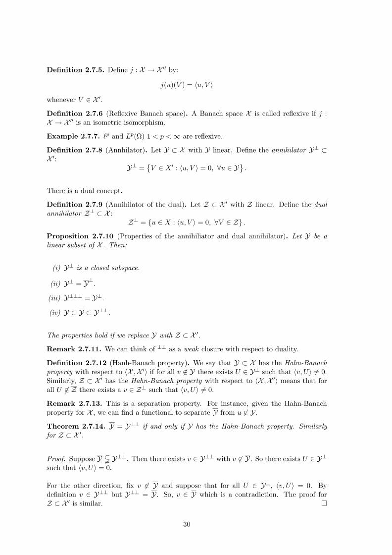
Definition 2.7.5. Define j : X → X by:

j(u)(V ) = u, V

whenever V ∈ X .

Definition 2.7.6 (Reflexive Banach space). A Banach space X is called reflexive if j :X → X is an isometric isomorphism.

Example 2.7.7. p and L

p(Ω) 1 < p < ∞ are reflexive.

Definition 2.7.8 (Annhilator). Let Y ⊂ X with Y linear. Define the annihilator Y⊥ ⊂X :

Y⊥ =

V ∈ X

: u, V = 0, ∀u ∈ Y

.

There is a dual concept.

Definition 2.7.9 (Annihilator of the dual). Let Z ⊂ X with Z linear. Define the dualannihilator Z⊥ ⊂ X :

Z⊥ = u ∈ X : u, V = 0, ∀V ∈ Z .

Proposition 2.7.10 (Properties of the annihiliator and dual annihilator). Let Y be alinear subset of X . Then:

(i) Y⊥ is a closed subspace.

(ii) Y⊥ = Y⊥.

(iii) Y⊥⊥⊥ = Y⊥.

(iv) Y ⊂ Y ⊂ Y⊥⊥.

The properties hold if we replace Y with Z ⊂ X .

Remark 2.7.11. We can think of ⊥⊥ as a weak closure with respect to duality.

Definition 2.7.12 (Hanh-Banach property). We say that Y ⊂ X has the Hahn-Banachproperty with respect to X ,X if for all v ∈ Y there exists U ∈ Y⊥ such that v, U = 0.Similarly, Z ⊂ X has the Hahn-Banach property with respect to X ,X means that forall U ∈ Z there exists a v ∈ Z⊥ such that v, U = 0.

Remark 2.7.13. This is a separation property. For instance, given the Hahn-Banachproperty for X , we can find a functional to separate Y from u ∈ Y.

Theorem 2.7.14. Y = Y⊥⊥ if and only if Y has the Hahn-Banach property. Similarlyfor Z ⊂ X .

Proof. Suppose Y Y⊥⊥. Then there exists v ∈ Y⊥⊥ with v ∈ Y. So there exists U ∈ Y⊥

such that v, U = 0.

For the other direction, fix v ∈ Y and suppose that for all U ∈ Y⊥, v, U = 0. Bydefinition v ∈ Y⊥⊥ but Y⊥⊥ = Y. So, v ∈ Y which is a contradiction. The proof forZ ⊂ X is similar.

30

Definition 2.7.15 (Hanh-Banach property on the whole space). We say that X or X

has the Hahn-Banach property with respect to X ,X if every linear subspace has theHahn-Banach property with respect to X ,X .

Theorem 2.7.16. (i) If X is separable then X has the Hahn-Banach property. Here,separable means that there is a countable dense subset.

(ii) Using the axiom of choice, a general space X has the Hahn-Banach property. (Hahn-Banach Theorem).

Remark 2.7.17. Note that for the space X , the Hahn-Banach property is still takenwith respect to X ,X , not X

,X . Assuming the axiom of choice the previous theoremtells us that the X has the Hahn-Banach property with respect to X

,X .

The situation generalises the special case when X is reflexive, where X ,X is equivalent

to X ,X . In fact, it is to generalise the reflexive condition why a “dual” formulation ofthe annihilator is necessary.

Theorem 2.7.18. Let Ω be a separable σ-finite measure space and 1 ≤ p < ∞. (Here Ωseparable means that the σ-algebra of measurable sets is generated by a countable sequenceof measurable sets). Then L

p(Ω) is separable.

Definition 2.7.19 (Dual operator with respect to X ,X ). Let S ∈ L (X ). DefineS ∈ L (X ) by:

v, SU = Sv, U

for all v ∈ X and U ∈ X .

Proposition 2.7.20. (S1S2) = S2S1

Let T ∈ L (X) and note that (T − λI) = (T − λI). We have:

Proposition 2.7.21. ρ (T ) ⊂ ρ (T ), σ (T ) ⊂ σ (T ) and

RT (ζ) = (RT (ζ))

We now relate this back to spectral projections. We are interested in determining whenX = N(T − λI)⊕ R(T − λI).

Proposition 2.7.22. (i) R(T − λI)⊥

= N(T − λI).

(ii) If X has the Hahn-Banach property, then N(T − λI) = R(T − λI)⊥.

(iii) If X has the Hahn-Banach property, R(T − λI)⊥

= N(T − λI).

(iv) If X has the Hahn-Banach property, then N(T − λI)⊥ = R(T − λI).

This leads immediately to the following theorem.

Theorem 2.7.23 (Spectral decomposition of the space). Let T ∈ L (X), and λ ∈ C.Suppose there exists ζn ∈ ρ (T ) such that ζn → λ and there exists a C > 0 such that|ζn − λ| RT (ζn) ≤ C. If both X and X have the Hahn-Banach property with respect toX ,X , then:

X = N(T − λI)⊕ R(T − λI).

31

Proof. By Theorem (2.6.7), we already have

X ⊃ X = N(T − λI)⊕ R(T − λI).

We have shown that ζn ∈ ρ (T ), so ζn → λ with the same resolvent bounds for T. It

follows thatX⊃ X = N(T − λI)⊕ R(T − λI).

Fix u ∈ X⊥. So, u ∈ N(T − λI)⊥ ∩ R(T − λI)⊥. By the previous proposition, we have:

N(T − λI) = R(T − λI)⊥

N(T − λI)⊥ = R(T − λI)

since X and X have the Hahn Banach property respectively. But this means that

u ∈ N(T − λI) ∩ R(T − λI) = 0

which makes X⊥ = 0. It follows that X⊥⊥ = X . Further, since X has the Hahn-Banachproperty, X⊥⊥ = X which establishes the result.

Remark 2.7.24. In particular, this decomposition holds if X is reflexive. For instance,for L

p(Ω) when 1 < p < ∞ and Ω ⊂ Rn.

Note, that this is not true for C[−1, 1] and L∞[−1, 1]. What about for L

1[−1, 1]?

32

Chapter 3

Unbounded Operators

We have so far considered operators that are bounded. But there are many useful operatorsthat are unbounded. The following is an important example to highlight this.

Example 3.0.25. Let X = L2(B), where B is an open ball in Rn. Define the Laplacian:

∆u =

j

∂2

∂x2j

u.

We can define various domains in L2(B):

(i) ∆0 : C∞c (B) → L

2(B).

(ii) ∆1 : W2,2(B) → L

2(B), where W2,2(B) =

u ∈ L

2(B) : ∂2u∂x2

j∈ L

2(B)

.

(iii) ∆D :u ∈ W

2,2(B) : u = 0 on ∂B→ L

2(B) (Dirichlet Laplacian).

(iv) ∆N =u ∈ W

2,2(B) : ∂u∂x = 0 on ∂B

→ L

2(B) (Neumann Laplacian).

These are four totally different operators. The first two operators do not even admit afunctional calculus.

3.1 Closed Operators

Definition 3.1.1 (General operator). Let X ,Y be Banach spaces. A linear operator T

from X to Y is a linear mapping T : D(T ) → Y where D(T ) is a linear subspace of X .

Remark 3.1.2. For a general operator, it is important to specify the domain D(T ).

Definition 3.1.3 (Closed operator). T is a closed operator means that the graph

G(T ) = (u, Tu) ∈ X × Y : u ∈ D(T )

is closed in X × Y. We usually simply say that T is closed.

33

Proposition 3.1.4. The following are equivalent:

(i) T is closed.

(ii) If un ∈ D(T ), un → u ∈ X and Tun → v ∈ Y then u ∈ D(T ) and Tu = v.

(iii) D(T ) is a Banach space under the graph norm given by:

u D(T ) = u + Tu .

Remark 3.1.5. Note that the graph norm looks similar to a Sobolev norm.

Definition 3.1.6 (Set of closed operators). We denote the collection of closed linearoperators from X to Y by C (X ,Y). We write C (X ) := C (X ,X ).

Remark 3.1.7. L (X ,Y) ⊂ C (X ,Y).

Definition 3.1.8. Let S, T ∈ C (X ,Y). We write S ⊂ T to mean G(S) ⊂ G(T ). That is,D(S) ⊂ D(T ) and Su = Tu for all u ∈ D(S).

Remark 3.1.9. C (X ,Y) is not a linear space. Note that ∆0 −∆0 = 0 since 0 is definedeverywhere. However, ∆0 − ∆0 ⊂ 0. It is in fact important to compute domains whenoperators are added and multiplied. The domains taken are the largest for which theconstructions make sense.

Proposition 3.1.10 (Domains). (i) (S+T )u = Su+Tu, u ∈ D(S+T ) = D(S)∩D(T ).

(ii) (ST )u = S(Tu), u ∈ D(ST ) = u ∈ D(T ) : Tu ∈ D(S).

(iii) If T : D(T ) → R(T ) is bijective, then D(T−1) = R(T ).

We list properties of operators in C (X ,Y).

Theorem 3.1.11 (Algebraic properties of closed operators). (i) S + T = T + S.

(ii) (S + T ) + U = S + (T + U).

(iii) S + 0 = S.

(iv) 0S ⊂ S0 = 0.

(v) S − S ⊂ 0.

(vi) (ST )U = S(TU).

(vii) S(T + U) ⊃ ST + SU .

(viii) (S + T )U = SU + TU

(ix) If S is bijective, S−1

S ⊂ I and SS−1 ⊂ I.

Proof. Exercise.

Also,

34

Proposition 3.1.12. Suppose B ∈ L (X ) and T ∈ C (X ). Then,

(i) TB ∈ C (X ).

(ii) If in addition B is bijective and B−1 ∈ L (X ), then BT ∈ C (X ).

(iii) If T is bijective, then T−1 ∈ C (X ).

Proof. (i) Let un ∈ D(TB), with un → u and TBun → v. Now, Bun → Bu by thebounded hypothesis. Also, wn = Bun ∈ D(T ) and wn → Bu and Twn → v. So,v = TBu.

We leave (ii) and (iii) as an exercise.

We want to start examining the spectral properties of closed operators. We start with anotion of invertibility.

Definition 3.1.13 (Invertible closed operator). T ∈ C (X ,Y) is invertible means:

(i) T is bijective with R(T ) = Y.

(ii) T−1 ∈ L (Y,X ).

Proposition 3.1.14. Let S ∈ C (X ,Y) with S invertible. Let B ∈ L (X ,Y) such that

B <1

S−1 .

Then, (S −B) is invertible and

(S −B)−1 ≤

S−1

1− B S−1

.

Proof. We note BS−1 ∈ L (Y ) and

BS−1

≤ B S

−1 < 1. Then,

I −BS−1

≤S

−1

1− BS−1 ≤

S−1

1− B S−1

.

So, S − B = S − BS−1

S = (I − BS−1) and (I − BS

−1) is bounded and invertible and(S −B)−1 = S

−1(I −BS−1)−1.

Definition 3.1.15 (Resolvent operator and resolvent set of a closed operator). If T ∈

C (X ) \ L (X ). Then ζ ∈ ρ (T ) means that (ζI − T ) is invertible. As before, we call ρ (T )the resolvent set of T and RT (ζ) = (ζI − T )−1 ∈ L (X) the resolvent operator. If furtherT ∈ L (X ) then ∞ ∈ ρ (T ).

Proposition 3.1.16. RT ∈ H(ρ (T ) ,L (X)).

Proof. As before, except for the case when T ∈ L (X) where we get ∞ ∈ ρ (T ). We leavethis as an exercise.

35

Corollary 3.1.17. ρ (T ) is an open subset of C.

Proof. Let ζ ∈ ρ (T ) and fix µ ∈ C such that

|µ− ζ| <1

(ζI − T )−1 .

Note that (µI−T ) = (ζI−T )+(µ− ζ)I, so apply previous proposition with B = (µ− ζ)Iand S = (ζI − T ) to find that (µI − T ) is invertible.

In order to discuss the spectrum of a closed operator, we need to define the extendedcomplex plane.

Definition 3.1.18 (Extended Complex plane). We write C∞ = C∪∞ for the extendedcomplex plane. We topologise this by saying that U is open in C∞ if either

(i) U is open in C.

(ii) U = C∞ \K, where K C.

Definition 3.1.19 (Spectrum of a closed operator). The definition is unchanged if T ∈

L (X). When T ∈ C (X) \ L (X), define

σ (T ) = C∞ \ ρ (T ) .

Remark 3.1.20. The spectrum of a T ∈ L (X ) is consistent with the previous definition.

Proposition 3.1.21. σ (T ) is nonempty.

Proof. We have already proved this for T ∈ L (X). When T ∈ C (X) \ L (X), ∞ ∈

σ (T ).

3.2 Functional calculus for closed operators

We have seen that while T ∈ C (X), the resolvent operator RT (α) ∈ L (X). The idea is tomap σ (T ) to some σ (S) with S bounded and define an H(Ω) functional calculus by theprevious Dunford-Riesz functional calculus for the operator S.

In general, closed operators may have σ (T ) = C∞, but we will not be discussing these.Unless otherwise stated, we assume that ρ (T ) = ∅.

Definition 3.2.1. Fix α ∈ C. Define Rα : C∞ → C∞ by:

Rα(µ) =

1µ−α µ = α, µ = ∞

∞ µ = α

0 µ = ∞

Proposition 3.2.2. Rα is a homeomorphism.

36

Proof. Exercise.

Proposition 3.2.3. Let α ∈ ρ (T ). Then,

−Rα(σ (T )) = σ (RT (α))

or equivalently,−Rα(ρ (T )) = ρ (RT (α)) .

Also, for ζ ∈ ρ (T ) where ζ ∈ α,∞, setting µ = −Rα(ζ), we have

µ(RRT (α)(µ) = (α− ζ)RT (ζ) + I.

Proof. The equivalence is a direct consequence of the previous proposition that Rα is ahomeomorphism.

Fix ζ ∈ ρ (T ). If ζ = α, then µ = ∞ and so µ ∈ ρ (RT (ζ)) since RT (ζ) is bounded.

Suppose ζ = ∞. This means that T is bounded and (αI − T ) ∈ L (X) which holds if andonly if RT (α) is invertible, that is, if and only if µ = 0 ∈ ρ (RT (α)).

Now, suppose ζ ∈ ρ (T ) \ α,∞. Then, µ ∈ 0,∞. So,

W =1µ

[(α− ζ)RT (ζ) + I] ∈ L (X ) .

We claim that[µ− RT (α)]W = W [µ− RT (α)] = I.

which we this as an exercise.

We also leave the proof of−Rα(σ (T )) ⊂ σ

RRT (α)

as an exercise.

Definition 3.2.4 (Holomorphic functional calculus for closed operators). Let T ∈ C (X )and Ω an open set in C∞ such that σ (T ) ⊂ Ω C∞. An H(Ω) functional calculus of T

is a mapping ΦT : H(Ω) → L (X ) such that

(i) ΦT is an algebra homomorphism and ΦT (1) = I.

(ii) There exists α ∈ C∞ such that:

ΦT (Rα) = −RT (α)ΦT (id) = T.

if α = ∞.

(iii) If fn → f uniformly on compact subsets of Ω, then fn(T ) → f(T ) in L (X ).

Remark 3.2.5. Note that the statement ΦT (id) = T along with ΦT (1) = id is equivalentto the definition of an H(Ω) functional calculus when T is bounded.

37

Theorem 3.2.6 (Existence and uniqueness of a functional calculus for closed operators).Such a functional calculus exists and it is unique.

Proof. Fix f ∈ H(Ω). Then, (f (−Rα)−1) ∈ H(−Rα(Ω)). Define ΦT by:

ΦT (f) := (f (−Rα)−1)(RT (α)) = (f R−1α )(−RT (α)) = Φ−RT (α)(f R

−1α ).

Since Φ−RT is the previous bounded functional calculus, the only thing we need to showis ΦT (Rα) = −RT (α). But this follows easily:

ΦT (Rα) = (Rα R−1α )(−RT (α)) = id(−RT (α)) = −RT (α).

As before, we typically write f(T ) := ΦT (f) in the light of the previous theorem. We listthe following important properties of the H(Ω) functional calculus we have defined.

Theorem 3.2.7 (Properties of H(Ω) functional calculus for closed operators). (i) ΦT (r) =r(T ) where r ∈ H(Ω) is a rational function.

(ii) When T ∈ L (X ), ΦT agrees with the H(Ω) functional calculus defined in §2.3.

(iii) Let Ω1,Ω2 be open sets in C∞ and suppose σ (T ) ⊂ Ω = Ω1 ∩Ω2. If f1 ∈ H(Ω1) andf2 ∈ H(Ω2) and f1 = f2 on Ω, then f1(T ) = f2(T ).

(iv) σ (f(T )) = f(σ (T )).

(v) There exists a C > 0 such that

f(T ) ≤ C f ∞

whenever f ∈ H∞(Ω).

(vi) If g ∈ H(Ω) and f ∈ H(Ω) where σ (g(T )) = g(σ (T )) ⊂ Ω, then

(f g)(T ) = f(g(T )).

(vii) If f1, f2 ∈ H(Ω), then

f1(T )f2(T ) = (f1f2)(T ) = f2(T )f1(T ).

(viii) We still have uniqueness if we replace axiom (iii) in the definition of the H(Ω) calculuswith:

(iii’) If fn → f uniformly on compact sets of Ω, then fn(T )u → f(T )u for all u ∈ X .

The spectral projections for the bounded operators also apply to closed operators. How-ever, in this situation, we also need to give consideration to the point ∞.

Theorem 3.2.8 (Spectral decomposition of a closed operator). Let T ∈ C (X ), α ∈ ρ (T ),α = λ ∈ C∞ and there exists a C > 0 and a sequence ζn ∈ ρ (T ) such that ζn → λ. Then,

38

(i) Suppose λ = ∞ and |ζn − λ| RT (ζn) ≤ C. Then, defining

Xλ = u ∈ X : ζn − λRT (ζn)u converges in X

we have the decomposition

X ⊃ Xλ = N(T − λI)⊕ R(T − λI).

(ii) Suppose λ = ∞ and |ζn| RT (ζn) ≤ C. Let wn = −Rα(ζn). Then, defining

X∞ = u ∈ X : (I − ζnRT (α)(ζn))u converges in X

we haveX ⊃ X

∞ = D(T ).Also, we have the characterisation

D(T ) = R(RT (α)) = u ∈ X : ζnRT (ζn)u → u = u ∈ X : TRT (ζn)u → 0

Furthermore, if X ,X have the Hahn-Banach property with respect to X ,X , then X λ =X .

Proof. (i) Either we can check that the proof for bounded operators works for closedoperators, or we can simply transfer the results by applying the result for boundedoperators to RT (α).

(ii) Again, we can redo the proof as for bounded operators or transfer the results toRT (α). We take the latter approach.We show that we have resolvent bounds at 0 = −Rα(∞) for the operator RT (α). Wenote that

wnRRT (α)(wn) = (α− ζn)RT (ζn) + I = I − ζnRT (ζn) + αRT (ζn)

By the resolvent bound for T at ∞, αRT (ζn) → 0 and we have the resolvent bound

|wn|RRT (α)(wn)

≤ C + 2.

Also,X∞ =

u ∈ X : wnRRT (α)(wn)u converges in X

.

It follows then that X ⊃ X∞ = N(RT (α)) ⊕ R(RT (α)) but since RT (α) is bijective,N(RT (α)) = 0. Also,

R(RT (α)) = D(RT (α)−1) = D(αI − T ) = D(T )

which proves the result.

We have the following important consequence.

Corollary 3.2.9 (Densely defined closed operator). If X ,X have the Hahn-Banach prop-erty with respect to X ,X , then T is a densely defined operator.

Typically, from now on, we consider operators with spectrum in a sector or a bisector.Our special points are 0,∞. The Ω are larger sectors that do not contain 0,∞.

39

Chapter 4

Sectorial Operators

So far, we have considered a functional calculus when σ (T ) ⊂ Ω ⊂ C∞.

Now, suppose T = ∆, the Laplacian on X = L2(Rn), which has spectrum, σ (∆) = [0,∞].

We want to look at e−t∆ but f(ζ) = e

−tζ is not holomorphic at ∞. Also, we want e−t√

∆

but f(ζ) = e−t√

ζ is not holomorphic at 0.

So we look at operators T such that:

(i) σ (T ) is contained in a “sector.” Then we consider Ω to be a slightly larger sectorwithout the points 0,∞.

(ii) σ (T ) is contained in a double sector and we take Ω to be a slightly larger doublesector not containing 0,∞.

The first situation (i) generalises the theory of ∆, and (ii) generalises

0 div−∇ 0

.

4.1 The Ψ functional calculus

Definition 4.1.1 (Sector). Let 0 ≤ ω < π. Define the closed ω sector :

Sω+ = ζ ∈ C∞ : | arg ζ| ≤ ω or ζ = 0,∞ .

Let 0 < µ < π. Define the open µ sector :

Soµ+ = ζ ∈ C : | arg ζ| < µ or ζ = 0 .

Definition 4.1.2 (ω-Sectorial operator). Let 0 ≤ ω < π. We say that T : D(T ) → X isan ω-sectorial operator if:

(i) T ∈ C (X ).

40

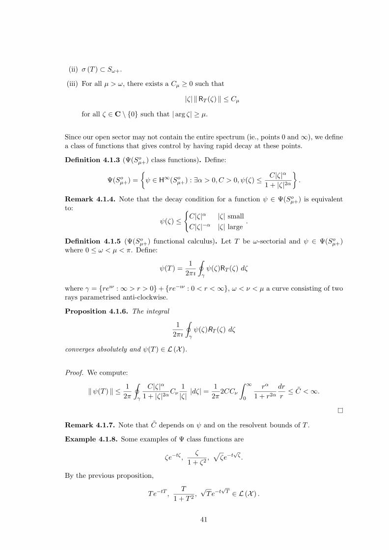
(ii) σ (T ) ⊂ Sω+.

(iii) For all µ > ω, there exists a Cµ ≥ 0 such that

|ζ| RT (ζ) ≤ Cµ

for all ζ ∈ C \ 0 such that | arg ζ| ≥ µ.

Since our open sector may not contain the entire spectrum (ie., points 0 and ∞), we definea class of functions that gives control by having rapid decay at these points.

Definition 4.1.3 (Ψ(Soµ+) class functions). Define:

Ψ(Soµ+) =

ψ ∈ H

∞(Soµ+) : ∃α > 0, C > 0, ψ(ζ) ≤

C|ζ|α

1 + |ζ|2α

.

Remark 4.1.4. Note that the decay condition for a function ψ ∈ Ψ(Soµ+) is equivalent

to:

ψ(ζ) ≤

C|ζ|α |ζ| smallC|ζ|−α |ζ| large

.

Definition 4.1.5 (Ψ(Soµ+) functional calculus). Let T be ω-sectorial and ψ ∈ Ψ(So

µ+)where 0 ≤ ω < µ < π. Define:

ψ(T ) =1

2πı

γψ(ζ)RT (ζ) dζ

where γ = reıν : ∞ > r > 0+ re−ıν : 0 < r < ∞, ω < ν < µ a curve consisting of tworays parametrised anti-clockwise.

Proposition 4.1.6. The integral

12πı

γψ(ζ)RT (ζ) dζ

converges absolutely and ψ(T ) ∈ L (X ).

Proof. We compute:

ψ(T ) ≤12π

γ

C|ζ|α

1 + |ζ|2αCν

1|ζ|

|dζ| =12π

2CCν

∞

0

rα

1 + r2α

dr

r≤ C < ∞.

Remark 4.1.7. Note that C depends on ψ and on the resolvent bounds of T .

Example 4.1.8. Some examples of Ψ class functions are

ζe−tζ

,ζ

1 + ζ2,

ζe−t√

ζ.

By the previous proposition,

Te−tT

,T

1 + T 2,

√Te

−t√

T∈ L (X ) .

41

Theorem 4.1.9 (Properties of the Ψ(Soµ+) functional calculus). (i) The definition of ψ(T )

is independent of ν ∈ (ω, µ).

(ii) Let ψ ∈ Ψ(Soµ+) and fix µ ∈ (ω, µ]. Let ψ = ψ|So

µ+. Then,

ψ(T ) = ψ(T ).

(iii) Ψ(Soµ+) → L (X ) is an algebra homomorphism.

(iv) If σ (T ) is compact in Soµ+ (ie., if 0 ∈ ρ (T ) and T ∈ L (X )), then ψ(T ) agrees with

the functional calculus in §2.3.

(v) If ψ ∈ H∞(Ω) where Ω is an open set satisfying S

oµ+ ∪ 0,∞ ⊂ Ω, then ψ(T ) agrees

with the functional calculus in §3.2.

(vi) Let ψn, ψ ∈ Ψ(Soµ+) and suppose there exists constants α > 0 and C > 0 such that

for all n,

|ψn(ζ)| ≤C|ζ|α

1 + |ζ|2α

and that ψn → ψ uniformly on compact subsets of Soµ+. Then, ψn(T ) → ψ(T ) in

L (X ).

Proof. (i) Fix ω < µ < µ, and let γ, γ be corresponding contours. We introduce “cuts”

δ+ε (t) = εe

tµ+(1−t)µ, 0 ≤ t ≤ 1

andδ+N (t) = Ne

tµ+(1−t)µ, 0 ≤ t ≤ 1

Now,

δ+ε

ψ(ζ)RT (ζ) dζ

≤ Cl(δ+ε )

εα

1 + ε2α

1ε≤ Cε

α

which tends to 0 as ε → 0. Similarly,

δ+N

ψ(ζ)RT (ζ) dζ

≤ C1

Nα

which tends to 0 as N →∞. We can similarly define δ−ε and δ

−N and show that

δ−ε

ψ(ζ)RT (ζ) dζ

,

δ−N

ψ(ζ)RT (ζ) dζ

→ 0

as ε → 0, and N →∞. We leave it as an exercise to check that this proves the claim.

(vi) Let γa,b = ζ ∈ γ : a ≤ |ζ| ≤ β. For N > δ > 0,

γ = γ0,δ + γδ,N + γN,∞.

42

Then,

2π ψn(T )− ψ(T ) ≤

γ0,δ

[ψn(ζ)− ψ(ζ)]RT (ζ) dζ

+

γδ,N


+

γN,∞


.

Fix ε > 0. Firstly, we can choose δ > 0 small such that

γ0,δ


< C

δ

0rα 1r

dr = C

δ

0rα−1 =

C

αδα

<2πε

3.

Then, we can choose N > δ > 0 large so that

γδ,N


< C

∞

N

1rα

1r

<2πε

3.

Now, there exists an M > 0 such that for n > M ,

γN,∞


<

N

δ|ψn(ζ)−ψ(ζ)|

1|ζ|

|dζ| ≤ C supζ∈γδ,N

|ψn(ζ)−ψ(ζ)| <2πε

3.

Combining these three estimates, we have that whenever n > M , ψn(T )− ψ(T ) <

ε which completes the proof.

As before, we get a splitting of the space with respect to the operator. However, forsectorial operators, it is also useful to consider the splitting with respect to the two points0,∞.

Proposition 4.1.10 (Splitting of the space with an ω-sectorial operator). Let T be anω-sectorial operator. Then,

(i) X ⊃ X 0 = N(T )⊕ R(T ).

(ii) X ⊃ X∞ = D(T ).

(iii) X ⊃ X 0,∞ = N(T )⊕ (R(T ) ∩ D(T )) where X 0,∞ = X 0 ∩ X∞.

(iv) D(T ) ∩ R(T ) = R(T (I + T )−1).

(v) D(T ) ∩ R(T ) = D(T ) ∩ R(T ) = R(T (I + T )−2).

As before, we have equality in (i)-(iii) if X ,X have the Hahn-Banach property with respectto X ,X .

43

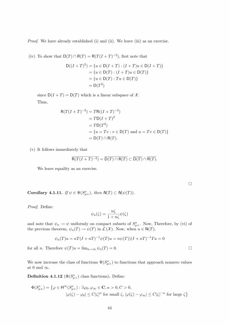
Proof. We have already established (i) and (ii). We leave (iii) as an exercise.

(iv) To show that D(T ) ∩ R(T ) = R(T (I + T )−2), first note that

D((I + T )2) = u ∈ D(I + T ) : (I + T )u ∈ D(I + T )= u ∈ D(T ) : (I + T )u ∈ D(T )= u ∈ D(T ) : Tu ∈ D(T )

= D(T 2)

since D(I + T ) = D(T ) which is a linear subspace of X .

Thus,

R(T (I + T )−2) = TR((I + T )−2)

= TD(I + T )2

= TD(T 2)= u = Tv : v ∈ D(T ) and u = Tv ∈ D(T )= D(T ) ∩ R(T ).

(v) It follows immediately that

R(T (I + T )−2) = D(T ) ∩ R(T ) ⊂ D(T ) ∩ R(T ).

We leave equality as an exercise.

Corollary 4.1.11. If ψ ∈ Ψ(Soµ+), then N(T ) ⊂ N(ψ(T )).

Proof. Define:

ψn(ζ) =nζ

1 + nζψ(ζ)

and note that ψn → ψ uniformly on compact subsets of Soµ+. Now, Therefore, by (vi) of

the previous theorem, ψn(T ) → ψ(T ) in L (X ). Now, when u ∈ N(T ),

ψn(T )u = nT (I + nT )−1ψ(T )u = nψ(T ))(I + nT )−1

Tu = 0

for all n. Therefore ψ(T )u = limn→∞ ψn(T ) = 0.

We now increase the class of functions Ψ(Soµ+) to functions that approach nonzero values

at 0 and ∞.

Definition 4.1.12 (Φ(Soµ+) class functions). Define:

Φ(Soµ+) =

ϕ ∈ H

∞(Soµ+) : ∃ϕ0, ϕ∞ ∈ C, α > 0, C > 0,

|ϕ(ζ)− ϕ0| ≤ C|ζ|α for small ζ, |ϕ(ζ)− ϕ∞| ≤ C|ζ|

−α for large ζ

44

Proposition 4.1.13 (Characterisation of Φ(Soµ+) functions). ϕ ∈ Φ(So

µ+) if and only ifthere exists a ψ ∈ Ψ(So

µ+) such that

ϕ(ζ) = ϕ0

1

1 + ζ

+ ϕ∞

ζ

1 + ζ

+ ψ(ζ) = ϕ∞ − (ϕ0 − ϕ∞)

1

1 + ζ

+ ψ(ζ).

Proof. Exercise.

Remark 4.1.14. Let Ω ⊃ Soµ+ ∪ 0,∞. Then Φ(So

µ+) ⊃ H(Ω) and Φ(Soµ+) ⊃ Ψ(So

µ+).

Proposition 4.1.15. Φ(Soµ+) is an algebra.

Proof. Exercise.

Definition 4.1.16 (Φ(Soµ+) functional calculus). Define Φ(So

µ+) → L (X ) functional cal-culus by:

ϕ(T ) = ϕ∞I − (ϕ0 − ϕ∞)RT (−1) + ψ(T )

whereψ(T ) =

12πı

γψ(ζ)RT (ζ) dζ.

Proposition 4.1.17. Φ(Soµ+) → L (X ) is an algebra homomorphism.

Proof. The only non-trivial step is to show that whenever ψ ∈ Ψ(Soµ+), and defining

f(ζ) =

11+ζ

ψ(ζ) ∈ Ψ(So

µ+), then

f(T ) = (I + T )−1ψ(T ).

We leave it as an exercise to verify that:

11 + ζ

RT (ζ) = −(I + T )−1

1

1 + ζI − (ζ − T )−1

.

Then,

f(T ) =1

2πı

γ

11 + ζ

ψ(ζ)RT (ζ) dζ

=1

2πı

γ−(I + T )−1 1

1 + ζψ(ζ) dζ +

12πı

γ(I + T )−1

ψ(ζ)RT (ζ) dζ

=−(I + T )−1

2πı

γ

11 + ζ

ψ(ζ) dζ + (I + T )−1 12πı

γψ(ζ)RT (ζ) dζ

= (I + T )−1ψ(T ).

The first term is zero by Cauchy’s Theorem.

Theorem 4.1.18 (Properties of the Φ(Soµ+) functional calculus). (i) Φ(So

µ+) → L (X )is an algebra homomorphism.

45

(ii) If σ (T ) is compact in Soµ+ (ie., if 0 ∈ ρ (T ) and T ∈ L (X )), then ϕ(T ) agrees with

the functional calculus in §2.3.

(iii) If ϕ ∈ H∞(Ω) where Ω is an open set satisfying S

oµ+ ∪ 0,∞ ⊂ Ω, then ϕ(T ) agrees

with the functional calculus in §3.2.

(iv) If ϕ(T ) ∈ Ψ(Soµ+) then, ϕ(T ) is the Ψ(So

µ+) functional calculus.

Remark 4.1.19. We have functions like e−tζ ∈ Φ(So

µ+), so we have e−tT ∈ L (X ). Note

that we still do not have estimates and we still cannot access a functional calculus offunctions ζ

is ∈ H∞(So

µ+).

We have the following important theorem.

Theorem 4.1.20 (The Convergence Lemma). Suppose fn ∈ Ψ(Soµ+) and there exists

C > 0 such that fn ∞ ≤ C for all n. Further, suppose f ∈ H∞(So

µ+) and that fn →

f uniformly on compact subsets of Soµ+. Also, suppose there exists C > 0 such that

fn(T ) ≤ C. Then, for all u ∈ X 0,∞ = N(T )⊕ (D(T ) ∩ R(T )), fn(T )u is a convergentsequence in X .

Proof. Firstly, suppose u ∈ N(T ). Then by Corollary 4.1.11, we have that fn(T )u → 0.

Now, fix u ∈ D(T )∩R(T ) By Prop 4.1.10 (iv), there exists v ∈ X such that u = T (I+T )−2v.

Define:ψn(ζ) =

ζ

(1 + ζ)2fn(ζ)

and so there exists a C> 0 such that

|ψn(ζ)| ≤ C |ζ|

1 + |ζ|2.

Setting

ψ(ζ) =ζ

(1 + ζ)2f(ζ)

we find that ψn → ψ uniformly on compact subsets of Soµ+. So, by Theorem 4.1.9,

ψn(T )v → ψ(T )v. So,

fn(T )u = fn(T )T (I + T )−2v = fn(T )u → ϕ(T )v.

By Prop 2.6.3, fn(T )u converges for all u ∈ R(T (I + T )−2) = D(T ) ∩ R(T ).

We leave the following further statements as exercises.

Remark 4.1.21. Suppose that the hypothesis of Theorem 4.1.20 are satisfied. Then,under the following additional hypothesis, we have the stronger consequences.

1. If f ∈ Φ(Soµ+), then whenever u ∈ D(T )∩R(T ), fn(T )u → f(T ) and when u ∈ N(T ),

fn(T )u → 0.

46

2. If α > 0 and |fn(ζ)| ≤ |C|ζ|α when ζ is small, then whenever u ∈ D(T ), fn(T )uconverges.

3. If α > 0 and |fn(ζ)| ≤ |C|ζ|−α when ζ is large, then whenever u ∈ N(T ) ⊕ R(T ),fn(T )u converges.

4. If (i) + (ii) holds, then fn(T ) → f(T ) on D(T ).

5. If (i) + (iii) holds, then fn(T ) → f(T ) on R(T ).

4.2 Semigroup Theory

In §2.5, we considered the family of operators (e−tT )0<t<∞ when T is a bounded operator.We now consider this theory where T is a sectorial operator.

More precisely, in this section, we fix µ and ω such that 0 ≤ ω < µ <π2 and we suppose

our operator is T ω-sectorial.

Proposition 4.2.1. Let ft(ζ) = e−tζ and let

ψt(ζ) =

e−tζ

−1

1 + tζ

.

Then, ψt ∈ Ψ(Soµ+) and

ft(ζ) =1

1 + tζ+ ψt(ζ).

Proof. We note that f ∈ Φ(Soµ+) and

|ψt(ζ)| ≤C|tζ|

1 + t2|ζ|2

which proves the assertion.

Definition 4.2.2 (Exponential Semigroup). Define:

e−tT = ft(T ) = (I + tT )−1 + ψt(T ).

Proposition 4.2.3. e−tT ∈ L (X ) for 0 < t < ∞.

Proof. Fix 0 < t < ∞. Then by resolvent bounds at 0, there exists a C > 0 such that

(I + tT )−1 =

−1tRT

−

1t

≤ C.

Also,

ψt(T ) ≤12π

γ|ψ(tζ)| |

dζ

ζ| =

12π

γ|ψ(ζ)| |

dζ

ζ| < ∞.

The result follows by combining these two estimates.

47

Proposition 4.2.4 (Properties of the Semigroup (e−tT )0<t<∞). (i) There exists a con-stant C > 0 such that

e−tT

≤ C whenever 0 ≤ t ≤ ∞.

(ii) e−tT

e−sT = e

−(t+s)T .

(iii) The semigroup is continous. That is, the mapping (0,∞) → L (X) defined by t →

e−tT is continuous.

(iv) The semigroup is differentiable in t, and

d

dte−tT = −Te

−tT⊃ −e

−tTT.

(v) If u ∈ N(T ), then e−tT

u = u.

(vi) If u ∈ R(T ), then limt→∞ e−tT

u = 0.

(vii) If u ∈ D(T ), then limt→0 e−tT

u = u.

(viii) u ∈ D(T ) if and only if

limt→0

1t(e−tT

u− u)

exists and−Tu = lim

t→0

1t(e−tT

u− u).

Proof. We have already proved (i), and (ii) is easy.

To prove (iii), fix a t0 ∈ (1,∞). We consider 12 t0 < t < 2t0. We already have that

(I + tT )−1 is continuous in t. Also, there exists and α > 0 such that

|ψt(ζ)| ≤C|ζ|α

1 + |ζ|2α

for ζ ∈ Soµ+, and in fact, uniformly bounded for our choice of t. Also, ψt → ψt as t → ∞

uniformly on compact sets and by applying Theorem 4.1.9, ψt(T ) → ψt0(T ) in L (X) whichestablishes continuity.

Now we prove (vi). Fix u ∈ R(T ). Firstly, note that

(I + tT )−1u = −

1tRT

−

1t

→ 0

since −1t → 0 as t →∞. Now, whenever 1 ≤ t < ∞, ψt → 0 uniformly on compact subsets.

That is, |ψt(ζ)| ≤ C|ζ| and ψt(T ) ≤ C and applying Corollary 4.1.11 ψt(T )u → 0.

We leave the rest as an exercise.

Remark 4.2.5. The last case, (viii) illustrates that

−T =d

dt|t=0 e

−tT

in the strong operator topology where we define ddt |t=0 as the limit in the theorem. We

say that −T is the generator of the semigroup.

48

What we have achieved has some far reaching consequences. We define the following“evolution equation.” We suppose that for simplicity that X = D(T ) = R(T ).

Definition 4.2.6 (Evolution Equation). Suppose there exists u : (0,∞) → L (X ) suchthat

ddtu(t) + Tu(t) = 0limt→0 u(t) = w

.

We say that u is an evolution equation.

Proposition 4.2.7. Given T an ω-sectorial operator (with ω <π2 ), there exists a unique

solution u to the evolution equation.

Proof. The solution is given by u(t) = e−tT

w. The solution is uniformly bounded in t:

u(t) ≤ C w .

Furthermore, u(t) → 0 as t →∞ and u(t) → w as t → 0. One can check that u is indeedunique.

So, this proposition shows that we have in fact solved an entire class of parabolic PDE. Inparticular, T = −∆ is the heat equation.

4.3 H∞ Functional Calculus

We return to the situation where our operator T is ω-sectorial with 0 ≤ ω < π.

Definition 4.3.1 (Bounded H∞ functional caculus). We say that T has a bounded

H∞(So

µ+) functional calculus if there exists C > 0 such that

ψ(T ) ≤ C ψ ∞

for all ψ ∈ Ψ(Soµ+).

A justification of this definition is necessary, because we have only considered Ψ(Soµ+) class

functions.

Proposition 4.3.2. Let f ∈ H∞(So

µ+). Then there exists a sequence ψk ∈ Ψ(Soµ+) and a

constant C > 0 such that ψk ∞ ≤ C and ψk → f uniformly on compact subsets of Soµ+.

Definition 4.3.3 (H∞(Soµ+) functional calculus). Fix f and let ψk ∈ Ψ(So

µ+) be a uni-formly bounded sequence such that ψk → f uniformly on compact subsets. Define:

f(T )u = limk→∞

ψk(T )u

for all u ∈ D(T ) ∩ R(T ).

Remark 4.3.4. The limit in the definition exists, since ψk(T )u is a cauchy sequencewhenever u ∈ D(T ) ∩ R(T ).

Proposition 4.3.5. f(T ) is well defined and there exists C > 0 such that f(T )u ≤C u for all u ∈ D(T ) ∩ R(T ).

49

Chapter 5

Operators on Hilbert Spaces

We start with a summary of Hilbert space theory. See for example [Hal98], [Kat76], [DS88].

Definition 5.0.6 (Inner Product). Let H be a linear space over C and let · , · : H×H→

C be a map satisfying:

(i) αu + βv, w = αu,w+ βv, w for all u, v, w ∈ H and α,β ∈ C.

(ii) u,αv + βw = αu, v+ βu,w for all u, v, w ∈ H and α,β ∈ C.

(iii) If u, v = 0 for all v then u = 0. (Positive definiteness)

Remark 5.0.7. An inner product is a notion of angle.

Definition 5.0.8 (Orthogonal). Let H be a linear space over C with an inner product· , · . Then, we say that u, v are orthogonal and write u ⊥ v if u, v = 0.

Remark 5.0.9. An inner product has an associated norm given by:

u =u, u.

Definition 5.0.10 (Hilbert Space). A Hilbert space is a linear space H over C with aninner product · , · which is a complete topological space with respect to the associatednorm.

Throughout this section, we will take H to mean a Hilbert space with an inner product· , · .

Proposition 5.0.11 (Properties of a Hilbert space).

(i) u, v = 14 [u + v − u− v + ı u + ıv − ı u− ıv ]. (Polarisation Identity)

(ii) u, v = v, u. (Hermitian)

(iii) |u, v| ≤ u v . (Cauchy-Schwartz)

(iv) u + v ≤ u + v . (Minkowski)

50

(v) u + v 2 + u− v

2 = 2 u 2 + 2 v

2. (Parallelogram)

(vi) Whenever u ⊥ v, u + v 2 = u

2 + v 2. (Pythagoras)

Example 5.0.12. (i) H = 2 with u, v =

∞i=1 ujvj .

(ii) H = L2(Ω) with u, v =

Ω uv.

The main theorem at the heart of Hilbert Space theory is the following.

Theorem 5.0.13 (Closest point). Let M ⊂ H be closed linear subspace. Then, for anyu ∈ H, there exists v ∈ M such that u− v = dist (u,M) and (u− v) ⊥ M .

Corollary 5.0.14. Let M⊥ = w ∈ H : w ⊥ v ∀v ∈ M. Then, H = M

⊥⊕ M

⊥ andM⊥⊥ = M .

Now, for the moment, let X be a Banach space. In §2.7, we considered the dual space tobe X = L (X ,C). That is, if f ∈ X , then f : X → C, bounded, and linear. In a Hilbertspace, it is often useful to replace this linearity with conjugate linearity.

Definition 5.0.15 (Adjoint space). Let X be a Banach space. Define:

X∗ = f : X → C conjugate linear .

Then, X ∗ is called the adjoint space of X .

Remark 5.0.16. It is worth noting that the theory we built for X in §2.7 works in muchthe same way if, instead, we worked with X ∗.

Theorem 5.0.17 (Reisz representation). Let u ∈ H and let fu ∈ H∗ be defined by fu(v) =

u, v for all v ∈ H. Then the map H→ H∗ given by u → fu is a linear isometry.

Proposition 5.0.18 (Hanh-Banach property of Hilbert spaces). Every Hilbert space H

has the Hahn-Banach property with respect to H,H∗.

Proof. Let M ⊂ H be a closed linear subspace. Let u ∈ H \ M . Then, we can writeu = v + w ∈ M ⊕M

⊥. Then, w = 0 and now consider fw ∈ H∗. Then, we have w ∈ M⊥

and fw(w) = w, w = w 2= 0. Also, if x ∈ M , fw(x) = w, x = 0.

5.1 The numerical range

From here on, we assume that T ∈ L (H).

Definition 5.1.1 (Numerical range, Numerical radius). Define the numerical range of T :

nr(T ) = Tu, u ∈ C : u ∈ H, u = 1 .

Define the numerical radius of T :

nrad(T ) = sup |nr(T )| = supu =0

|Tu, u|

u 2 .

51

Remark 5.1.2. Note that nrad(T ) ≤ T .

Proposition 5.1.3. 12 T ≤ nrad(T ) ≤ T .

Corollary 5.1.4. nr(T ) = λ if and only if T = λI.

Proof. nr(T ) = λ ⇐⇒ nr(T − λI) = 0 ⇐⇒ T − λiI = 0 ⇐⇒ T = λI.

Theorem 5.1.5 (Toeplitz-Hausdorff (1906)). The numerical range nr(T ) is convex.

Example 5.1.6. Let T =

0 10 0

. Then, σ (T ) = 0, T = 1. We compute the

numerical range:

nr(T ) =

0 10 0

α

β

,

α

β

∈ C : |α|2 + |β|

2 = 1

=βα ∈ C : |α|2 + |β|

2 = 1

.

The, the numerical radius is nrad(T ) = 12 .

Example 5.1.7. Let H = 2, λ = (λj)∞j=1, λj ∈ C and ||λ||∞ = supj |λj | < ∞. Define

T = diag(λj). Then, for u ∈ 2, (Tu)j = λjuj . Now, T = ||λ||∞ point spectrum (set

of eigenvalues) is σpt (T ) = λj and the spectrum is σ (T ) = σpt (T ). We compute thenumerical range:

nr(T ) = Tu, u ∈ C : u = 1 =

j

λjujuj :

j

|uj |2 = 1

.

We denote the convex hull of a set S (set of finite sums) by co(S). Then,

σpt (T ) ⊂ co(σpt (T )) ⊂ nr(T ) ⊂ co(σpt (T ))

andσ (T ) = σpt (T ) ⊂ co(σpt (T )) = nr(T ).

Also, in this example, nrad(T ) = T .

In particular, the preceding example highlights that σ (T ) ⊂ nr(T ), and not nr(T ). In fact,this is true in general, and we prove this as a theorem. But first, we need some resultsabout adjoints of operators.

Definition 5.1.8 (Adjoint). Let T ∈ L (H). We define T∗ : H→ H by T ∗u, v = u, Tv

for all u, v ∈ H.

Remark 5.1.9. In the general theory, the adjoint of an operator acts on the adjoint space,just as the dual of an operator acts on the dual space as see in §2.7. But this definitionmakes sense in the light of the Riesz representation theorem as we can identify the adjointspace H∗ with H.

Proposition 5.1.10 (Properties of the Adjoint). (i) T∗ ∈ L (H) and T

∗ = T .

(ii) T∗∗ = T and (αT + βS)∗ = αT

∗ + βT∗.

52

(iii) (ST )∗ = T∗S∗ and I

∗ = I.

(iv) If S is invertible, then S∗ is invertible and (S∗)−1 = (S−1)∗.

(v) ζ ∈ ρ (T ) if and only if ζ ∈ ρ (T ∗) and RT (ζ)∗ = RT ∗(ζ).

(vi) λ ∈ σ (T ) if and only if λ ∈ σ (T ).

(vii) α ∈ nr(T ) if and only if α ∈ nr(T ∗).

(viii) H = N(T )⊥⊕ R(T ∗).

Proof. (i) Note that,

T∗ = sup

u,v =0

|T ∗u, v|

u v = T .

(viii) We have

u ∈ N(T ) ⇐⇒ Tu, v = 0 ∀v ∈ H⇐⇒ u, T

∗v = 0 ∀v ∈ H

⇐⇒ u ⊥ R(T ∗)

⇐⇒ u ⊥ R(T ∗)

We leave the rest as an exercise.

Proposition 5.1.11. Let T ∈ L (H). If α,β ≥ 0 such that

(i) u ≤ α Tu for all u ∈ H

(ii) v ≤ β T∗v for all v ∈ H

then T is bijective, T−1 ∈ L (H) and

T−1

≤ min α,β .

Proof. Condition (i) immediately gives that T is one-one with closed range. Condition(ii) gives that T

∗ is one-one and so N(T ∗) = 0. It follows by (viii) and (ii) of Proposition5.1.10 that R(T ) = H. Putting these two facts together gives that R(T ) = H and soT−1 ∈ L (H). Furthermore, (i) gives that

T−1

w ≤ α w . Using the same argument,

we can find that T∗−1

∈ L (H) andT

∗−1w

≤ β w . Since T = T∗ , it follows

thatT

−1 ≤ min α,β.

We now return to prove the general statement that σ (T ) ⊂ nr(T ).

Theorem 5.1.12. Let T ∈ L (H). Then,

(i) σ (T ) ⊂ nr(T ).

53

(ii) For all ζ ∈ C \ nr(T ),

RT (ζ) ≤1

dist (ζ,nr(T )).

Proof. Fix ζ ∈ C \ nr(T ). let d = dist (ζ,nr(T )). Then, for all u ∈ H \ 0,ζ −

Tu, u

u 2

≥ d.

By Cauchy-Schwartz and multiplying across by u 2,

(ζI − T )u u ≥ |(ζI − T )u, u| ≥ d u 2.

So, u ≥1d (ζI − T )u u . Similarly, we apply the same argument with T

∗ in placeof T and ζ in place of ζ to find the estimate u ≥

1d

(ζI − T∗)u

u . By Proposition5.1.11, we get R(ζI −T ) = H and (ζI −T )−1 ∈ L (H) so ζ ∈ ρ (T ) proving σ (T ) ⊂ nr(T ).Also, by the same proposition,

RT (ζ) ≤1d

=1

dist ζ,nr(T )

which completes the proof.

5.2 Functional calculus and numerical range

Let p(ζ) =N

k=0 αkζk. We define p(ζ) =

Nk=0 αkζ

k. Note that p(ζ) = p(ζ). Then, notethat

p(T )∗ = (N

k=0

αkTk)∗ =

N

k=0

αkT∗k = p(T ).

We use the case of polynomials as a prototype to consider the “conjugation” of an arbitraryfunction f .

Definition 5.2.1 (Conjugate function). Let Ω ⊂ C, Ω open and let Ωconj =ζ : ζ ∈ Ω

,

the conjugate of Ω. Then, whenever f ∈ H(Ω), we define f ∈ H(Ωconj) by f(ζ) = f(ζ).

Proposition 5.2.2. f(T )∗ = f(T ).

Remark 5.2.3. Suppose Ω is connected and Ω ∩R = ∅. Then,

f(ζ) = f(ζ) ∀ζ ∈ Ω ⇐⇒ f(x) = f(x) ∀x ∈ Ω ∩R ⇐⇒ f(x) ∈ R ∀x ∈ Ω ∩R

Definition 5.2.4 (Self adjoint). We say that T ∈ L (H) is a self adjoint operator ifT = T

∗.

Proposition 5.2.5. T = T∗ if and only if nr(T ) ⊂ R.

Proof. To prove that when T = T∗ then nr(T ) ⊂ R, observe that

Tu, u = T∗u, u = u, Tu = Tu, u.

We leave the other direction as an exercise.

54

Proposition 5.2.6. There exists a, b ∈ R, satisfying a ≤ b such that nr(T ) = [a, b] ornr(T ) = a. Moreover, a, b ∈ σ (T ), so that nr(T ) = co(σ (T )) and T = nrad(T ) =sup |σ (T ) |.

Theorem 5.2.7. Let T be self adjoint and suppose Ω is open in C, nr(T ) ⊂ Ω. Supposethat f ∈ H(Ω) such that f = f . Then, f(T ) is self adjoint and

f(T ) ≤ supζ∈nr(T )

|f(ζ)| ≤ f ∞ .

Proof. Firstly, we observe that f(T )∗ = f(T ∗) = f(T ). Now,

f(T ) = sup |σ (f(T )) | = sup |f(σ (T ))| = supζ∈σ(T )

|f(ζ)| ≤ supζ∈nr(T )

|f(ζ)| ≤ f ∞

Exercise 5.2.8. Prove that the preceding theorem remains true without the conditionf = f .

Remark 5.2.9. In fact, for self adjoint operators, we have a Borel functional calculusvia the spectral representation. Furthermore, the estimate f(T ) ≤ f ∞ holds for allBorel measurable functions f : σ (T ) → C.

5.3 Accretive operators

Definition 5.3.1 (Accretive). An operator T ∈ L (H) is called accretive if Re Tu, u ≥ 0for all u ∈ H.

Proposition 5.3.2. T ∈ L (H) is accretive if and only if T + T∗ is a non negative self

adjoint operator

Proof. Note that

ReTu, u ≥ 0 ∀u ∈ H ⇐⇒ Tu, u+ u, Tu ≥ 0 ∀u ∈ H⇐⇒ (T + T

∗)u, u ≥ 0 ∀u ∈ H⇐⇒ T + T

∗ is non-negative self adjoint.

which establishes the claim.

In particular, this theorem tells us that there exists√

T + T ∗ ∈ L (H). Also, we find√

T ∈ L (H) by integrating around the numerical range and using the resolvent bounds at0.

Also, for a bounded accretive operator T , by considering ft(ζ) = e−tζ for t > 0, we find e

−tT ≤ 1. That is, we get a contraction semigroup. In fact, this works even when T is

unbounded.

55

Definition 5.3.3 (Bounded strictly accretive). An operator T ∈ L (H) is called strictlyaccretive if there exists κ > 0 such that ReTu, u ≥ κ u

2 for all u ∈ H.

Theorem 5.3.4. Suppose that T is a bounded strictly accretive operator, and let µ >π2 .

If f ∈ H∞(So

µ+), then

f(T ) ≤ 1· supζ∈ıR

|f(ζ)| = 1· supRe ζ≥0

|f(ζ)|.

Proof. Let ψ ∈ Ψ(Soµ+). We can take γ = −ıR since µ >

π2 and then

ψ(T ) =1

2πı

γψ(ζ)(ζI − T )−1

dζ

=1

2πı

ıRψ(ζ)[(T − ζI)−1 + (T ∗ + ζI)−1

dζ (Since (T ∗ + ζI)−1 is holomorphic on Soµ+)

=1

2πı

ıR(T ∗ + ζI)−1(T ∗ + T )(T − ζI)−1

dζ

Now, there exists ψn ∈ Ψ(Soµ+) such that ψn → f uniformly on compact subsets of S

oµ+.

So, ψn(T ) → f(T ). By the decay condition on (T ∗ + ζI)−1(T ∗ + T )(T − ζI)−1,

f(T ) =12π

∞

−∞f(ıy)(T ∗ + ıyI)−1(T ∗ + T )(T − ıyI)−1

dy

and

f(T )u, v =12π

∞

−∞f(ıy)(T ∗ + T )

12 (T − ıyI)−1

u, (T ∗ + T )12 (T − ıyI)−1

v dy

for all u, v ∈ H.

Putting f ≡ 1, u = v, we get,

u 2 =

12π

∞

−∞

(T ∗ + T )12 (T − ıyI)−1

u

2

dy.

By the application of Cauchy-Schwartz,

|f(T )u, v| ≤12π

supy∈R

|f(iy)| ∞

−∞

(T ∗ + T )12 (T − ıyI)−1

u

(T ∗ + T )

12 (T − ıyI)−1

v

dy

≤ supζ∈ıR

|f(ζ)|

12π

∞

−∞

(T ∗ + T )12 (T − ıyI)−1

u

2

dy

12

12π

∞

−∞

(T ∗ + T )12 (T − ıyI)−1

v

2

dy

12

= supζ∈ıR

|f(ζ)| u v

Definition 5.3.5 (Bounded ω-accretive). Let 0 ≤ ω <π2 . We say an operator T ∈ L (H)

is bounded ω-accretive if nr(T ) ⊂ Sω+.

56

Note that T is ω-accretive means that T is π2 -accretive, which is the same as saying that

T is accretive.

Proposition 5.3.6. T ∈ L (H) is bounded strictly accretive implies there exists ω <π2

such that T is bounded and ω-accretive.

Proof. Note that |nr(T )| ≤ T . Let κ > 0 be the constant in the strict accretivehypothesis. Then, take ω such that T cos ω = κ.

Proposition 5.3.7. T ∈ L (H) bounded strictly accretive implies that T−1 is bounded

strictly accretive.

Proof. Firstly, we note that the strict accretive hypothesis implies that 0 ∈ ρ (T ) so thatRT (0) = T

−1 ∈ L (H). Also,

RT (0) ≤1

dist (0,nr(T ))≤

1κ

.

Since T is also ω-accretive with some ω <π2 ,

T−1

u, u = T−1

u, TT−1

u = T (T−1u), (T−1u) ∈ Sω+.

So,Re T−1

u, u = Re T (T−1u), (T−1

u) ≥ κT

−1u

2≥

κ

T u

2.

Example 5.3.8. (i) Let H = 2, and let T = diag(λj)∞j=1. We already know that

nr(T ) = co λj. Then, T is bounded strictly accretive if and only if |λj | ≤ ω andRe λj ≥ κ > 0 for all j.

(ii) Let H = L2(Rn). Let b ∈ L

∞(Rn) such that Re b(x) ≥ κ > 0 for almost everyx ∈ Rn. Let T be the map u → bu. Then, T = b ∞ and

ReTu, u = Re

Rnb(x)|u(x)|2 dx ≥ κ u

2.

(iii) Let H = L2(Rn

,CN ), and T ∈ L∞(Rn

, MN×N ) such that ess sup|T (x)| = T ∞ <

∞, and Re T (x) ≥ κI for almost all x ∈ Rn. Then, T ∈ LL

2(Rn,CN )

defined by

Tu(x) = T (x)u(x) is bounded strictly accretive.

5.4 Closed operators

Let H,K be Hilbert spaces. Let T ∈ C (H,K) and suppose that D(T ) = H.

Definition 5.4.1 (Adjoint). The adjoint T∗ of T is the operator with the largest domain

D(T ∗) such that Tu, v = u, T∗v for all u ∈ D(T ), v ∈ D(T ∗).

57

Remark 5.4.2. Equivalently, we could define

D(T ∗) = v ∈ K : ∃f ∈ H s.t. Tu, v = u, f ∀u ∈ D(T )

andT∗v = f.

This is indeed well defined. Suppose there exists g ∈ H such that

Tu, v = u, f = u, g

for all u ∈ D(T ). Then, f = g if and only if D(T ) is dense in H. This is why we made thethe density assumption on D(T ).

Remark 5.4.3. Note thatH⊕K = G(T )

⊥⊕ G(−T

∗)

since(u, Tu), (−T

∗v, v) = −u, T

∗v+ Tu, v = 0.

This gives us another approach to define the adjoint. Take G(T )⊥ in H ⊕ K and check ifit is the graph of an operator. Clearly such is the case if T is densely defined. So, define−T

∗ to be the operator with the corresponding graph G(T )⊥. See [Kat76].

Proposition 5.4.4 (Properties of T∗). (i) T

∗ ∈ C (K,H).

(ii) D(T ∗) = K.

(iii) T∗∗ = T .

(iv) H = N(T )⊥⊕ R(T ∗) and K = N(T ∗)

⊥⊕ R(T ).

(v) If T is invertible (ie,. T−1 ∈ L (K,H)), then T

∗ is invertible and T∗−1 = T

−1∗.

(vi) ζ ∈ ρ (T ) ⇐⇒ ζ ∈ ρ (T ∗) and RT (ζ)∗ = RT ∗(ζ).

(vii) λ ∈ σ (T ) ⇐⇒ λ ∈ σ (T ∗).

Proof. We prove (ii). Suppose u ∈ D(T ∗)⊥. That is u, v = 0 for all v ∈ D(T ∗) which is ifand only if (0, u), (−T

∗v, v) = 0 for all v ∈ D(T ∗) in H⊕K. So, (0, u) ∈ G(−T

∗)⊥ = G(T )which implies u = 0. So, D(T ∗) = K.

The rest of the proposition is left as an exercise.

Remark 5.4.5. Unlike in the case for bounded operators, we do not always have thatnr(T ) = nr(T )conj. This is because the domains D(T ) and D(T ∗) may be different, even inthe case H = K.

Definition 5.4.6 (Self adjoint). T ∈ C (H) self adjoint means that T is densely definedand T = T

∗.

Remark 5.4.7. As a consequence, D(T ) = D(T ∗). Also, σ (T ) ⊂ nr(T ) ⊂ R and for allζ ∈ C \R,

RT (ζ) ≤1

Im ζ.

58

Definition 5.4.8 (ω-accretive operator). Let 0 ≤ ω ≤π2 . Then, we say that T is ω-

accretive if

(i) T ∈ C (H),

(ii) nr(T ) ⊂ Sω+,

(iii) σ (T ) ⊂ Sω+.

Remark 5.4.9. Note that condition (ii) is equivalent to saying that | argTu, u| ≤ ω forall u ∈ D(T ). When, T ∈ L (H), (ii) implies (iii).

Proposition 5.4.10. Suppose T satisfies (i) and (ii) in the definition of ω-accretivity.Then whenever ζ ∈ C \ nr(T ), we have (T − ζI)u ≥ dist (ζ, Sω+) u . So T − ζI isinjective with closed range.

Remark 5.4.11. In this case, (iii) holds if and only if R(T − ζI) = H. The proof is bythe stability of the semi-Fredholm index.

Proposition 5.4.12. If T is ω-accretive, then

RT (ζ) ≤1

dist (ζ, Sω+)

for all ζ ∈ C \ Sω+ and T is ω-sectorial.

Remark 5.4.13. An immediate consequence is that D(T ) = H and H = N(T ) ⊕ R(T ).(Note that ⊕ does not imply orthogonality.)

Theorem 5.4.14. Suppose that (i) and (ii) holds. Then, (iii) holds (ie., T is ω-accretive)if and only if D(T ) = H and nr(T ∗) ⊂ Sω+.

Proof. Suppose that D(T ) = H and nr(T ∗) ⊂ Sω+. Then, (T ∗ − ζI)−1

u ≥ dist (ζ, Sω+) u

whenever ζ ∈ Sω+. So, (T ∗− ζI) is injective which implies that N(T ∗− ζI) = 0. It followsthat R(T − ζI) = H which implies ζ ∈ ρ (T ). This proves σ (T ) ⊂ Sω+.

To prove the other direction, suppose T is ω-accretive. By the previous theorem, ω-accretive implies ω-sectorial and we have that D(T ) = H. Fix ε > 0. Then, (T + εI) isω-accretive and (T + εI)−1 is bounded and ω-accretive. So, (T ∗ + εI)−1 is bounded andω-accretive and nr(T ∗ + εI) ⊂ Sω+. Then let ε → 0 to conclude nr(T ∗) ⊂ Sω+.

We summarise the properties of ω-accretivity.

Proposition 5.4.15 (Properties of ω-accretivity). Let T be ω-accretive. Then,

(i) Whenever ζ ∈ Sω+, we have

RT (ζ) ≤1

dist (ζ, Sω+).

59

(ii) T is ω-sectorial.

(iii) H = N(T )⊕ R(T ).

(iv) If T is injective, then R(T ) = H.

(v) D(T ) = H.

(vi) T has a bounded H∞ functional calculus, and whenever ψ ∈ Ψ(So

µ+) for µ >π2 ,

ψ(T ) ≤ 1· ψ ∞ .

Remark 5.4.16. We can get bounds for even more general f , for instance, ft(ζ) = etζ ,

and we find e

−tT ≤ 1. For a general f ∈ H

∞(Soµ+) with µ > ω, we can show f(T ) ≤

C f ∞

Example 5.4.17. LetH = L2[0,∞), and let T = d

dx with D(T ) = u ∈ H : u ∈ H, u(0) = 0 =

W1,20 [0,∞).

Now, T ∈ C (H), and D(T ) = H. Also, T∗ = −

ddx with D(T ∗) = u ∈ H : u

∈ H =W

1,2[0,∞). Formally,

Tu, v = ∞

0uv = −

∞

0uv + 0 = u, T

∗v.

Then, the numerical range is nr(T ) = Tu, u : u ∈ D(T ) and

Re Tu, u =12

uu +

uu

=

12

uu + uu

= 0.

So, nr(T ) ⊂ ıR (in fact = ıR) and T satisfies (i) and (ii) in the definition of π2 -accretive.

Note that

(T ∗ − λI)u = 0 ⇐⇒ −u− λu = 0, u ∈ H(0,∞) ⇐⇒ u(x) = Ce

λx.

So, (T ∗ − λI) is 1-1 if and only if Re ζ = Re ζ ≤ 0 and this happens if and only ifR(T − λI) = H. Therefore, we conclude that T is π

2 -accretive.

Note that if we instead considered the operator −T , then it would satisfy (i), (ii) but not(iii).

The following is the main example.

Example 5.4.18 (Uniformly elliptic divergence form PD operator). Let H = L2(Rn),

κ > 0 and A ∈ L∞(Rn

, Mn×n) such that Re A(x)w, w ≥ κ|w|2 for almost all x ∈ Rn

and for all w ∈ Cn.

Define an associated sesquilinear form

J [u, v] =

RnA(x)∇u(x),∇v(x) dx

60

for all u, v ∈ W1,2(Rn). Now, we have that J [u, u] ∇u

2.

We can think of J as being a complex energy. We think of ∇ as the unbounded operator∇ : L

2(Rn) → L2(Rn

,Cn) where

∇f = (∂1f, . . . , ∂nf)

with D(∇) = W1,2(Rn). Similarly, we consider div : L

2(Rn,Cn) → L

2(Rn) defined by

div u =n

j=1

∂juj

with D(div ) =u ∈ L

2(Rn,Cn) : div u ∈ L

2(Rn). Then, div = −∇∗. This is because

∇f, u =

Rn

n

j=1

∂jfuj = −

Rn

n

j=1

f∂juj = f,div u.

The operator associated with the form J is the operator L with the largest domain D(L)such that

J [u, v] = Lu, v

for all u ∈ D(L) and for all v ∈ D(J) = W1,2(Rn).

We find that D(L) ⊂ W1,2(Rn). In fact, even without this fact, we have

Lu, u = J [u, u] =

RnA(x)∇u(x),∇u(x) dx ∈ Sω+.

By Lax-Milgram Theorem, we find σ (L) ⊂ Sω+. In other words, L is ω-accretive.

Furthermore, L∗ = −div A

∗∇.

5.5 Fractional powers

Definition 5.5.1 (Fractional Powers). Let T be a ω-sectorial operator and 0 < α < 1.Define

Tα = (I + T )ψα(T )

whereψα(ζ) =

ζα

1 + ζ∈ Ψ(S0

µ+)

for µ > ω. Define T0 = I and T

1 = T .

We list the important properties of fractional powers.

Proposition 5.5.2 (Properties of fractional powers of T ). Let T be an ω-sectorial opera-tor. Then,

61

(i) Tα is αω-sectorial.

(ii) TαT

β = Tα+β as long as α + β ≤ 1.

(iii) In particular, if α = 12 , then we write

√T = T

12 and it is the unique ω

2 operatorsatisfying

√T√

T = T .

(iv) D(T ) ⊂ D(√

T ) ⊂ H.

(v) (Tα)∗ = (T ∗)α.

(vi) If T is ω-accretive, then Tα is αω-accretive.

We leave the proof of this as an exercise.

Example 5.5.3. We return to Example 5.4.18. Recall that L = −div A∇ and L∗ =

−div A∗∇. Now, assume that ω = 0 so that A is self adjoint. Then L = L

∗ and so√

L∗ =

√L∗ =

√L. Also,

√

Lu

2

= √

Lu,

√Lu

†= Lu, u = A∇u,∇uL2 ∇u 2

for all u ∈ D(L) and from this it follows that

u 2 +

√

Lu

2 u

2 + ∇u 2 u

2W 1,2 .

By a density argument we can show that D(√

L) = W1,2(Rn) with equivalent norms.

But this is all for self-adjoint operators and it is well known classical theory. In the nonself-adjoint case, the equality † fails.

This was the question that was asked by Kato in 1961. Suppose ω = 0. Then is thefollowing true?

D(√

L) = W1,2(Rn) with

√

Lu

∇u

In 1972, McIntosh gave a negative answer in the case that A is not multiplication. It wasnot until 2002 that the question was answered by Auscher, Hofmann, Lacey, McIntosh andTchamitchian. See [AHL+02].

5.6 Bisectorial operators

In this section, let 0 ≤ ω <π2 .

Definition 5.6.1 (Sω−, Soµ−, Sω, S

oµ). Define the left closed sector Sω− = −Sω+. and the

left open sector Soµ− = −S

oµ+. Then, the closed bisector is defined as Sω = Sω+ ∪Sω− and

the open bisector Soµ = S

oµ+ ∪ S

oµ−.

62

Definition 5.6.2 (Bisectorial operator). T ∈ C (H) is called an ω-bisectorial operator if

(i) σ (T ) ⊂ Sω, and

(ii) For all µ > ω (µ <π2 ), there exists a constant Cµ > 0 such that

RT (ζ) ≤Cµ

|ζ|

for all ζ ∈ C \ Sµ.

Remark 5.6.3. As before, we have H = N(T ) ⊕ R(T ) and H = D(T ) because resolventbounds at 0 and ∞ are unchanged.

Proposition 5.6.4. If T is ω-bisectorial, then T2 is 2ω-sectorial. In particular,

√T 2 is

ω-sectorial.

Proof. Firstly, note that ζ ∈ C \ S2µ if and only if ±√

ζ ∈ C \ Sµ. By the ω-bisectorialityof T , there exists a Cµ such that

RT (±

ζ) ≤

Cµ

|√

ζ|.

Now, (ζI − T2) = −(

√ζI − T )(−

√ζI − T ) and so it follows that

RT 2(ζ) ≤Cµ

|√

ζ|

Cµ

|√

ζ|=

C2µ

|ζ|.

Proposition 5.6.5. Let A, A−1 ∈ L (H) and S ∈ C (H). Then ASA

−1 ∈ C (H) andASA

−1 − ζI = A−1(S − ζI)A.

A direct consequence is the following.

Corollary 5.6.6. If S ∈ C (H) and A ∈ L (H) with A invertible, then σASA

−1

=σ (S). If S is ω-(bi)sectorial then ASA

−1 is ω-(bi)sectorial. Furthermore, f(A−1SA) =

A−1

f(S)A.

Theorem 5.6.7. Suppose S = S∗ ∈ C (H) and B ∈ L (H) strictly ω-accretive. Then SB

and BS are ω-bisectorial. Moreover, if S ≥ 0 then they are ω-sectorial.

Proof. Let ζ ∈ C \ Sω. Then,B

−1 (ζI −BS)u u ≥ |B

−1(ζI −BS)u, u|

= |ζB−1

u, u − Su, u|

= |B−1

u, u||ζ −Su, u

B−1u, u|

63

for all u ∈ D(S). Since S is self adjoint, Su, u ∈ R, and by the ω-accretivity hypothesison B,

Su, u

B−1u, u∈ Sω.

It follows that,

|B−1

u, u|

ζ −Su, u

B−1u, u

≥κ

B 2 u

2 dist (ζ, Sω).

So,

(ζI −BS)u ≥κ

2

B 2 dist (ζ, Sω) u

for all u ∈ D(S) which implies that (ζI −BS) is one-one with closed range. Also,

(ζI −BS)∗ = (ζI − (BS)∗) = (ζI − SB∗) = B

∗−1(ζI −B∗S)B∗

.

By a similar argument as before, (ζI − B∗S) is one-one and so R(ζI −BS) = H. This

implies that ζ ∈ ρ (BS) and

RBS(ζ) ≤B

2

κ2

1dist (ζ, Sω)

.

The result for SB follows from Corollary 5.6.6 on noting that SB = B−1(BS)B. We used

the fact that (BS)∗ = SB∗. We leave this as an exercise.

5.7 Bounded H∞ functional calculus of bisectorial operators

Definition 5.7.1 (Ψ(Soµ) class and Ψ(So

µ) functional calculus). Let T be an ω-bisectorialoperator and let µ > ω with µ <

π2 . Define

Ψ(Soµ) =

ψ ∈ H

∞(Soµ) : ∃α > 0, C ≥ 0 s.t. |ψ(ζ)| ≤

C|ζ|α

1 + |ζ|2α

.

For ψ ∈ Ψ(Soµ), define

ψ(T ) =1

2πı

γψ(ζ)RT (ζ) dζ

where

γ = teıν : ∞ > t > 0+

−te

−ıν : 0 < t < ∞+teıν : ∞ > t > 0+

te−ıν : 0 < t < ∞

with ω < ν < µ.

As for sectorial operators, we have the following result.

Proposition 5.7.2 (Properties of the Ψ(Soµ) functional calculus). (i) The integral

ψ(T ) =1

2πı

γψ(ζ)RT (ζ) dζ

converges absolutely in L (H).

64

(ii) The definition of ψ(T ) is independent of γ.

(iii) The map Ψ(Soµ) → L (H) defined by ψ → ψ(T ) is an algebra homomorphism.

Further properties are analogous to those of ω-sectorial operators. We just note:

Theorem 5.7.3 (The Convergence Lemma for bisectorial opeators). Suppose fn ∈ Ψ(Soµ),

f ∈ H∞(So

µ), there exists C ≥ 0 such that fn ∞ ≤ C and that fn(T ) ≤ C. If fn → f

uniformly on compact subsets of Soµ, then fn(T )u converges for all u ∈ H.

Remark 5.7.4. Note that if u ∈ N(T ), then fn(T )u = 0 → 0.

Definition 5.7.5 (Bounded H∞(So

µ) functional calculus). We say that an ω-bisectorialoperator has bounded H

∞(Soµ) functional calculus if there exists a C ≥ 0 such that for all

ψ ∈ Ψ(Sµ),ψ(T ) ≤ C ψ ∞ .

We define the following important class of functions.

Definition 5.7.6 (H∞(Soµ, 0)). Define

H∞(So

µ, 0) =

f : Soµ ∪ 0→ C; f |So

µ∈ H

∞(Soµ)

.

Remark 5.7.7. Notice that a function f ∈ H∞(So

µ, 0) is typically not holomorphic oreven continous at 0.

Definition 5.7.8 (H∞(Soµ, 0) functional calculus). A bounded H

∞(Soµ, 0) functional

calculus is a map ΦT : H∞(So

µ, 0) → L (H) satisfying:

(i) ΦT is an algebra homomorphism.

(ii) ΦT is bounded. That is, there exists a C > 0 such that ΦT (f) ≤ C f ∞.

(iii) ΦT (1) = 1 and ΦT (Rα) = −RT (α).

(iv) If fn, f ∈ H∞(So

µ, 0) and there exists a C > 0 such that fn ∞ ≤ C and fn(ζ) →f(ζ) for all ζ ∈ S

oµ ∪ 0, then fn(T )u → f(T )u.

We write f(T ) = ΦT (f).

The following equivalence is important.

Proposition 5.7.9. An ω-bisectorial operator T has a bounded H∞(So

µ) functional calculusif and only if T has a bounded H

∞(Soµ, 0) functional calculus.

Lemma 5.7.10. Let f ∈ H∞(So

µ). Then, there exists a sequence fn ∈ Ψ(Soµ) such that

fn ∞ ≤1

cos2 µ f ∞ and fn → f uniformly on compact subsets of Soµ.

65

Proof. Letϕn(ζ) =

ın

ın + ζ

andϕn(ζ) =

ζ

ın + ζ

.

Then, ϕn ∞ , ϕn ∞ ≤1

cos µ . Also,|ϕn(ζ) ≤ |ζ|−1 for |ζ| large and |ϕn(ζ)| ≤ |ζ| when|ζ| small. Define ψn = ϕnϕn and ψn ∈ Ψ(So

µ) with ψn ≤1

cos2 µ . Then, ψn(ζ) → 1 foreach ζ ∈ S

oµ. Set fn = ψnf and notice that fn(ζ) → f(ζ) pointwise and therefore, fn → f

uniformly on compact subsets. Also, fn ∞ ≤1

cos2 µ f ∞.

Proposition 5.7.11. Suppose that T has a bounded H∞(So

µ) functional calculus and letP

T0 : H→ N(T ) denote the projection onto the null space. If f ∈ H

∞(Soµ, 0), then,

f(T )u = f(0)P T0 u + lim

n→∞fn(T )u

where fn ∈ Ψ(Soµ) with fn → f uniformly on compact subsets, fn ∞ ≤ C f ∞ where

C can depend on µ.

Remark 5.7.12. By the Convergence Lemma, fn(T )u converges for all u ∈ H.

Corollary 5.7.13. The functional calculus H∞(So

µ, 0) → L (H) defined by f → f(T ) isunique.

We can now consider decomposing the space according to spectral subspaces somewhatanalogous to what we did in §2.4.

Definition 5.7.14 (χ±, χ0, sgn). Define χ±, χ0, sgn ∈ H∞(So

µ, 0) by

χ±(ζ) =

1 ζ ∈ S

oµ±

0 otherwise

and

χ0(ζ) =

1 ζ = 00 otherwise

.

Then, we define sgn = χ+ − χ−.

Proposition 5.7.15. If T has a bounded H∞(So

µ) functional calculus, then, χ±(T ), χ0(T ), sgn(T ) ∈L (H). Also, χ±(T ), χ0(T ) are projections that satisfy χ±(T )χ∓(T ) = χ±(T )χ0(T ) = 0.Furthermore,

χ0(T )u = PT0 u = lim

n→∞

ı

nRT

ı

n

u.

Proof. By application of Cor 5.7.13 we have χ±(T ), χ0(T ), sgn(T ) ∈ L (H) by noting thatχ±, χ0 ∈ H

∞(Sµ, 0).

Then, note that χ2± = χ±, χ

20 = χ0, χ±χ∓ = 0, χ±χ0 = 0 and apply the algebra homo-

morphism property of the functional calculus.

The formula χ0(T ) = limn→∞ınRT

ın

follows since it is the projection into N(T ).

66

Definition 5.7.16 (Spectral Projections). Define P± = χ±(T ) and P0 = χ0(T ) andH± = R(P±).

We have the following important splitting of the space into spectral subspaces.

Proposition 5.7.17. If T has a bounded H∞ functional calculus, then H = N(T )⊕H+⊕

H−.

We leave the proof of the following important proposition as an exercise.

Proposition 5.7.18. Whenever T has a bounded H∞ functional calculus,

sgn(T )T =√

T 2

T = sgn(T )√

T 2

andTu

√

T 2u

for all u ∈ H.

So far, we have assumed that T has a bounded H∞ functional calculus. However, not all

ω-bisectorial operators have a H∞ functional calculus. We give three examples of operators

that do have a bounded H∞ functional calculus.

Example 5.7.19.

T = diag(λj) in 2 where λj ∈ Sω.

T = Mϕ in L2(Ω), ϕ ∈ L

∞(Ω) with ess ranϕ ⊂ Sω.

That these operators have a bounded H∞ functional calculus is a relatively easy fact. The

following is a much deeper result related to current research. See [AMK].

Theorem 5.7.20. Let T = BD in H = L2(Rn

,CN ), N ≥ 1, with B ∈ L∞(Rn

, MN×N ) =

L∞(Rn

,LCN

) with Re B ≥ κI, where κ > 0. Let D be a homogeneous first order partial

differential operator with constant coefficients satisfying D = D∗ and Du ∇ ⊗ u ,

when u ∈ R(D).

Example 5.7.21. Suppose N = n + 1 so H = L2(Rn)⊕ L

2(Rn,Cn) and

B =

I 00 A

, D =

0 −div∇ 0

where A satisfies the condition in Example 5.4.18.

Then, BD has a bounded H∞ functional calculus and BDu

(BD)2u. When

u = (f, 0), this gives √−div A∇f

∇f

which is the Kato square root problem.

67

Consider the following evolution equation.

(E)

d

dtU(t) + DBU(t) = 0

U(0) = u ∈ H

If u ∈ H+, then there exists a unique solution U ∈ C1(R+

,H) such that U(t) → 0 ast →∞ and U(t) → u as t → 0. Namely, this solution is

U(t) = e−tDB

u = e−t√

(DB)2u

because DB =

(DB)2 on H+.

If u ∈ H−, then there is a unique solutions U ∈ C1(R−

,H) and it is given by

U(t) = e−tDB

u = et√

(DB)2u, t < 0

because DB = −

(DB)2 on H−.

Now, if u ∈ N(T ), the U = u for all t ∈ R.

The following very special case is well known. We present it to acknowledge the roots ofthe subject.

Example 5.7.22. Let H = L2(R), D = 1

ıddx , and B = I. Suppose we set the initial

condition U(0) = 0. Then,

(E) ⇐⇒ ∂tU +1ı∂xU = 0

⇐⇒ ∂xU +1ı∂tU

⇐⇒ U is holomorphic

u ∈ H+ if and only if Du =√

D2u. This happens if and only if ξu(ξ) = |ξ|u(ξ) whichis if and only if sppt u ⊂ [0,∞). Similarly, u ∈ H− if and only if sppt u ⊂ (−∞, 0]. So,u ∈ H+ if u extends to a holomorphic function on the upper half plane. Similarly u ∈ H−if u extends to a holomorphic function on the lower half plane.

Also, sgn(D)Du =√

D2u and (ξu) = |ξ|u(ξ). So, sgn(D) = H is the Hilbert transform,which is given by

sgn(D)u =1πı

p.v. ∞

−∞

u(x)x− y

dx.

68

Bibliography

[ADM96] D. Albrecht, X. Duong, and A. McIntosh, Operator theory and harmonic anal-ysis, Instructional Workshop on Analysis and Geometry, Part III (Canberra,1995), Proc. Centre Math. Appl. Austral. Nat. Univ., vol. 34, Austral. Nat.Univ., Canberra, 1996, pp. 77–136.

[AHL+02] P. Auscher, S. Hofmann, M. Lacey, A. McIntosh, and Ph. Tchamitchian, Thesolution of the Kato square root problem for second order elliptic operators onRn, Ann. of Math. (2) 156 (2002), no. 2, 633–654.

[AM] Axelsson A. Auscher, P. and A. McIntosh, On a quadratic estimate related tothe kato conjecture and boundary value problems.

[AMK] A. Axelsson, A. McIntosh, and S. Keith, Quadratic estimates and functionalcalculi of perturbed Dirac operators, CMA Research Report MRR04-006.

[DS88] N. Dunford and J. T. Schwartz, Linear operators. Part I, Wiley Classics Li-brary, John Wiley & Sons Inc., New York, 1988.

[Hal98] Paul R. Halmos, Introduction to Hilbert space and the theory of spectral multi-plicity, AMS Chelsea Publishing, Providence, RI, 1998, Reprint of the second(1957) edition. MR MR1653399 (99g:47001)

[Kat76] T. Kato, Perturbation theory for linear operators, second ed., Springer-Verlag,Berlin, 1976, Grundlehren der Mathematischen Wissenschaften, Band 132.

[Lor62] Edgar Raymond Lorch, Spectral theory, University Texts in the MathematicalSciences, Oxford University Press, New York, 1962. MR MR0136967 (25 #427)

[Rem98] Reinhold Remmert, Classical topics in complex function theory, Graduate Textsin Mathematics, vol. 172, Springer-Verlag, New York, 1998, Translated fromthe German by Leslie Kay. MR MR1483074 (98g:30002)

[RS72] Michael Reed and Barry Simon, Methods of modern mathematical physics. I.Functional analysis, Academic Press, New York, 1972. MR MR0493419 (58#12429a)

[RSN90] Frigyes Riesz and Bela Sz.-Nagy, Functional analysis, Dover Books on Ad-vanced Mathematics, Dover Publications Inc., New York, 1990, Translated fromthe second French edition by Leo F. Boron, Reprint of the 1955 original. MRMR1068530 (91g:00002)

[Rud87] Walter Rudin, Real and complex analysis, third ed., McGraw-Hill Book Co.,New York, 1987. MR MR924157 (88k:00002)

69

[Sim83] George F. Simmons, Introduction to topology and modern analysis, Robert E.Krieger Publishing Co. Inc., Melbourne, Fla., 1983, Reprint of the 1963 original.MR MR695310 (84b:54002)

70

Notation

T∗ Adjoint operator of T .

L (X ,Y) Bounded linear functions from normed space X to Banach space Y equippedwith the operator norm.

L (X ) The space L (X ,X ).

C∞ Extended complex plane or Riemann sphere C∞ = C ∪ ∞.

C (X ,Y) Closed operators from X to Y.

co(S) Convex hull of S.

f The conjugation of the function f given by f(ζ).

∆ The Laplacian operator.

diag(λj) Matrix with the diagonal entry j set to λj .

p Infinite sequences with the p norm.

H(Ω) The space H(Ω,C).

H(Ω,X ) The space of all holomorphic functions from Ω to X .

H∞(Ω) Bounded holomorphic functions on open Ω ⊂ C.

H∞(Ω,X ) Space of bounded holomorphic functions from Ω to X .

id The identity map id : z → z.

· , · Inner product.

X ,X Duality of X and X under the bilinear pairing

v, U Bilinear pairing of v and U

X Banach Space.

X Dual space of X

X ∗ Adjoint space of X .

X1 ⊕ X2 Direct sum of Banach spaces X1 and X2.

71

Y⊥ The annihilator of Y

· V Norm on a space V .

nr(T ) Numerical range of T .

nrad(T ) Numerical radius of T .

Φ(Soµ+) Bounded holomorphic functions on the sector S

oµ+ that are constant at 0 and ∞.

P Algebra of polynomials.

PR Algebra of power series with radius of convergence larger than R.

Ψ(Soµ+) Holomorphic functions ψ decaying at a power α > 0 at 0, ∞

Ψ(Soµ) Holomorphic functions on the open bisector S

oµ.

RK Algebra of rational functions with no poles in K.

ρ(T ) Resolvent set of T .

RT Resolvent operator of T .

σp(T ) The point spectrum or the set of eigenvalues.

s- limn→∞ Sn The limit taken in the strong convergence topology.

σ (T ) The spectrum of T .

C0(M) Functions over a metric space M that decay at ∞.

Cb(M) Space of continuous complex valued bounded functions on a metric space M .

K Ω K compact and K ⊂ Ω.

Lp(Ω) Functions f : Ω → R with finite integral p norm.

MN×N The space of N ×N matrices

PT0 Projection H → N(T ).

S ⊂ T Operator T is an extension of S.

Sconj The complex conjugate of the set S.

Soµ+ Open µ-sector.

Soµ− The left open sector −S

oµ+.

Soµ The open bisector S

oµ+ ∪ S

oµ−.

Sω+ Closed ω-sector.

Sω− The left closed sector −Sω+.

Sω The closed bisector Sω+ ∪ Sω−.

u ⊥ v u is perpendicular to v, ie., u, v = 0.

Wp,k(Ω) The Sobolev space in L

p with k derivatives.

72

Index

Absolutely Convergent, 6Accretive

ω, 59Properties, 59

Bounded, 55ω-accretive, 56Strictly, 56

Adjoint, 52Closed operator, 57

Properties, 58Properties, 52

Adjoint space, 51Algebra

Polynomial, 17Power Series, 18Rational, 17

Annihilator, 30Dual, 30Properties, 30

Approximation by rationals, 14

Banach Algebra, 9unital, 9with identity, 9

Banach Space, 5Banach space

Direct sum, 7Direct sum of subsets, 7Reflexive, 30

Bilinear pairing, 29

Cauchy’s Theorem, 12Closest point theorem, 51Conjugate function, 54Contour

Closed, 9Contour integral, 9Curve

Piecewise Ck, 9

Definite (Riemann) integral, 8Densely defined closed operator, 39

Differentiable, 11Dual space, 29Duality, 29

Eigenvalue, 15Eigenvector, 15Exponential, 24

Family for ω-sectorial operators, 47Semigroup for ω-sectorial operators, 47Semigroup, properties, 48

Extended Complex plane, 36

Family of spectral projections, 23Fractional Powers

ω-sectorial operator, 61Properties, 61

Fractional powers, 24, 25Functional calculus

Φ(Soµ+), 45

Ψ calculus for sectorial operators, 40Ψ(So

µ+), 41H(Ω), 20H(Ω) for closed operators, 37H∞(So

µ+), 49Bounded H

∞, 49ω-bisectorial, 65

Composition, 22Dunford, 19Existence and uniqueness of H(Ω), 20Existence and uniqueness of H(Ω) for

closed operators, 38Holomorphic, 19Polynomial, 17Power series, 18Properties of H(Ω), 22Properties of H(Ω) for closed operators,

38Properties of Φ(So

µ+), 45Properties of Ψ(So

µ+), 42Properties of the Ψ(So

µ), 64Rational, 18

Hahn-Banach property, 30

73

Hilbert space, 51On the whole space, 31sufficient conditions, 31

Hilbert space, 50Properties, 50

Holomorphic, 11bounded, 13

Indefinite (Riemann) integral, 8Infinite Series, 5Inner product, 50

Associated norm, 50Integral p norm, 6Invertible, 9

Kato square root problem, 62, 67

Laplacian, 33Dirichlet, 33Neumann, 33

Liouville’s Theorem, 13

Numerical radius, 51Numerical range, 51, 53

Operatorω-Bisectorial, 63ω-Sectorial, 40Closed, 33

Domains, 34Extension, 34Invertible, 35Set, 34

Direct sum, 7General, 33Sectorial, 40Uniformly elliptic divergence form PD,

60Operator Norm, 6Orthogonal, 50

Power Series, 10Projection, 8

Rational function, 17Resolvent, 15

Bounds, 26Closed operator, 35holomorphicity, 16properties, 16Set of closed operator, 35

Resolvent set, 15Open, 16

Riesz representation theorem, 51Runge’s Theorem, 14

Sector, 40Bisector, 62Left closed, 62Right closed, 62

Self adjoint, 54Closed operator, 58

Semigroups, 47Spectral decomposition, 23, 27

ω-sectorial operator, 43Banach space, 23Closed operator, 38Operator, 23two points, 43Whole space, 31

Spectral mapping theorem, 22Spectral Projections, 26Spectrum, 15

Closed operator, 36Compact, 17Nonempty, 17properties, 16

Strong convergence, 26Sum p norm, 6

The Convergence Lemma, 46Bisectorial, 65

Toeplitz-Hausdorff theorem, 52

74

operator theory - spectra and functional...

Documents