operational diversification and stability of financial

Research Journal of Finance and Accounting www.iiste.org ISSN 2222-1697 (Paper) ISSN 2222-2847 (Online) Vol 3, No 3, 2012

70

Operational Diversification and Stability of Financial Performance in Indian Banking Sector: A Panel Data

Investigation Deepti Sahoo1 Pulak Mishra2*

1. Doctoral Research Scholar, Department of Humanities and Social Sciences, Humanities and Social Sciences, Indian Institute of Technology Kharagpur, Kharagpur – 721 302, India.

2. Associate Professor of Economics, Department of Humanities and Social Sciences, Humanities and Social Sciences, Indian Institute of Technology Kharagpur, Kharagpur – 721 302.

* E-mail of the corresponding author: [email protected]

Abstract

Reforms in Indian banking sector and subsequent entry of domestic and foreign private banks have enhanced competition in the sector significantly raisings the possibility of fluctuations in financial performance of the banks. As a strategic response to these changing market conditions, many of the banks have followed the route of diversifying their operations to reduce the instabilities in their financial performance. In this perspective, the present paper is an attempt to examine the impact of the strategy of operational diversification on stability in financial performance of the banks. The paper uses panel data regression techniques for a set of 59 banks over the period from 1995-96 to 2007-08. It is found that the banks with greater extent diversification of operations suffer from the problem of larger fluctuations in financial performance possibly due to their failure in deciding the right areas of diversification and its optimum extent. Future research should aim at addressing these issues as over-diversification of operations or diversification into areas of noncore competencies may affect stability of financial performance adversely as well as may create conflicts across the regulators in defining their jurisdiction, particularly when the areas of operations overlap.

Keywords: Operational diversification, financial performance, stability, banks, India

1. Introduction:

Reforms in Indian banking sector1and subsequent entry of domestic and foreign private banks have enhanced competition in the sector significantly raisings possibility of fluctuations in financial performance of the banks. This has resulted in a considerable change in the objectives, strategies, and operations of the banks. As a strategic response to the changing market conditions, policies, and regulations, many of the banks operating in India have taken the route of diversifying their operations to reduce the fluctuations in their financial performance. Increasingly, the banks are transcending their normal operations, and are venturing into the areas like insurance, investment and other non-banking activities2 . Deregulation, disintermediation, and emergence of advanced technologies, along with the consolidation wave in the sector have largely facilitated the banks to diversify their operations (Arora and Kaur, 2009). In addition, lowering of the Cash Reserve Ratio (CRR) and the Statutory Liquidity Ratio (SLR) has also enabled the banks to diversify their operations by enhancing flexibility in their business decisions.

1Major changes on the policy front include relaxing the restrictions on domestic investment, promoting foreign investment, opening up of capital market, simplification of different financial instruments, and diversification of investment sectors. 2 A large number of banks have undertaken traditionally non-banking activities such as investment banking, insurance, mortgage financing, securitization, and particularly, insurance (Jalan, 2002).


71

It is expected that diversification of operations would help the banks in leveraging managerial skills and abilities across services (Iskandar-Datta and McLaughlin, 2007), gaining economies of scope by spreading fixed costs (Steinherr and Huveneers 1990; Drucker and Puri, 2009), and providing a financial supermarket to customers who demand multiple products (Berger et al, 2010a). It is also likely to reduce the expected costs of financial distress or bankruptcy by lowering risks3 (Boot and Schmeits, 2000) as well as the chances of costly financial distress (Berger et al., 2010a). More importantly, the banks are designed to diversify by nature (Winton, 1999; Acharya et al. 2006). Since deregulation and the resulting intensified competition have forced the banks to engage in risk-taking activities for their market share or profit margins, diversification of operations may help them in spreading the risks of operations across different services, and thereby stabilizing financial performance. In addition, diversification of operations may also contribute to the stability in financial performance by providing opportunity to gain non-interest income, engaging in activities where returns are imperfectly correlated, and diluting the impact of priority sector lending.

However, diversification of operations into different services can affect performance of a bank adversely by reducing the comparative advantage of managerial expertise when it goes beyond their existing level (Klein and Saidenberg, 1998). This is very important, particularly when diversification of operations exposes the banks to various new risks4 and the management does not have the necessary expertise to control these risks efficiently. In addition, the banks may suffer due to diversification inducing competition as well (Winton, 1999). For the public-sector banks, it is also possible that engagement in the securities business would lead to concentration of market power in the sector due to their reputation and informational advantages, and this may restrict other banks from competing on a level playing field. Further, entering into underwriting services through diversification may lead to conflicts of interest between banks and the investors and this, in turn, may affect financial performance of the banks adversely. A wide body of literature (e.g., Jensen, 1986; Berger and Ofek, 1996; Servaes, 1996; Denis et al., 1997) point out that the financial institutions should focus on a single line of business, especially to reap the benefits of managerial expertise as well as to reduce the agency problem.

Thus, the existing studies do not show any consensus on the impact of operational diversification on financial performance of banks. For example, Xu (1996) finds that banks benefit from diversification in the form of greater stability of returns from their asset. It is observed that international banking with diversification of assets helps the banks to escape from systematic risks. In addition, diversification of operations also enhances efficiency of the banks (Landi and Venturelli, 2002)5. Movement into non-bank product lines also reduces risks of cash flow of the banks (Rose, 1989). Contrary to this, a focused strategy can raise profit and reduce risks only up to a certain threshold, and when foreign ownership is either very high or very low, banks tend to benefit more from being diversified (Berger et al, 2010b). Some other studies, that find lower risks following operational diversification include Santomero and Chung (1992), Saunders and Walter (1994), Kwan (1998), and Stiroh and Rumble (2006).

On the other hand, according to Templeton and Severiens (1992), operational diversification of the banks into other financial services would reduce unsystematic risks, but it does not affect systematic risks. Earning of the banks may become more volatile as they engage more in fee-based activities and move away from traditional intermediation activities (De Young and Roland, 1999). The banks which expand into non-interest income activities face a higher level of risks than the banks that are engaged mainly in traditional intermediation activities (Lepetit et al, 2005). Besides, mergers with insurance firms can reduce the risks of bankruptcy, but combinations with securities/real estate companies may raise possibility of the same (Boyd and Graham, 1988; Lown et al., 2000).When diversification fails to reduce risks, it may be because of

3 In the present paper, the term ‘risks’ indicates instabilities in financial performance.

4 For example, banks may end up buying the securities they underwrite. They may also face greater market risks as they increase their share of securities holdings and market-making activities. 5Landi and Venturelli (2002) observe a strong positive correlation between diversification and the X-efficiency score, in terms of both cost and profit.


72

lower capital ratios, larger commercial and industrial loan portfolios, and greater use of derivatives (Demsetz and Strahan, 1997). Further, greater reliance on non-interest income also results in more volatile returns and lower risk-adjusted profits for the banks (Stiroh, 2004a and 2004b).

Hence, there is no consensus on the nature of impact of operational diversification on stability in financial performance of the banks. Further, the existing studies are largely confined to the USA and the European countries, and examining the relationship in the context of transitional/emerging economies like India has remained largely unexplored6. More importantly, in Indian context, the direction of causality between diversification and risks of operation is not very clear. While the conventional wisdom suggests that the banks should diversify their operations to reduce risks, Arora and Kaur (2009) find that risks, cost of production, regulatory costs, and technological changes are the major determinants of diversification of operations in Indian banking sector. Similarly, Bhaduri (2010) observe that, with increased volatility of income following liberalization, the banks have gradually shifted their attention more towards other income related instruments.

The lack of consensus on the nature of impact of diversification on fluctuations in financial performance of the banks, and the direction of causality between the two in the existing studies raises an important question, should banks diversify across different services, or should they specialize? Addressing this debate on focus versus diversification is very important as the banks on many occasions face conflicting regulations and market conditions across sectors that may restrict their strategic flexibility as well as the benefits of diversification. In this perspective, the objective of the present paper is to examine the impact of operational diversification on stability of financial performance of the banks operating in India. The rationale for such attempt, particularly in Indian context arises as there is no robust policy framework stipulated by the Reserve Bank of India (RBI) to integrate diverse activities of the banks (Bhaduri, 2010), and in the absence of such policy resolution, increasing diversification of operations by the banks can result in conflicts amongst the regulators of different sector. The recent conflict between the Insurance Development and Regulatory Authority (IRDA) and the Securities and Exchange Board of India (SEBI) in regulating the unit-liked insurance policies (ULIPs) is a classic example in this regard. In addition, premature deregulation and foreign entry may increase the risks of crisis in the sector, especially when the macroeconomic and the regulatory structure are weak (Demirgüç-Kunt et al. 1998).

The rest of the paper is divided into four sections. Section 2 gives an overview on how the extent of operational diversification of Indian banks and the fluctuations in their financial performance have varied across the banks and over the period of time. The regression model estimated to examine diversification-risks relationship, measurement and possible impact of the independent variables, estimation techniques applied, and sources of data are discussed in Section 3. Section 4 presents the regression results and discusses the possible implications of the major findings. Section 5 concludes the paper.

2. Variations in Diversification and Financial Performance: An Overview

In banking sector, the term "diversification" is used to define multi-dimensionality in operations. The banks adopt the strategy of diversification primarily to reduce the risks. They also diversify their operations to grow their business, particularly when the prospect of growth in the present line of operation is limited. This growth may be realized by broadening the horizon of their services, i.e., by adding new services into their portfolio. The other motives of diversification by the banks may include gaining market power, maximizing value, strengthening capital base, etc. (Ali- Yrkko, 2002).

6 However, there are a few studies that have attempted to explore diversification-performance relationships in banking sector of the transitional economies. For example, Berger et al (2010a) have examined the effects of focus versus diversification on performance of Chinese banks. Similarly, Berger et al (2010b) have explored the relationship between diversification strategies and the risk-return trade-off in Russian banking sector.


73

The indices proposed and applied in the literature to measure diversification are largely similar to those used for measuring market concentration. The present paper uses two alternative measures of the extent of diversification, viz., Berry’s Index (DIV_BE) based on Berry (1971) and the Entropy index (DIV_EN) as suggested by Hart (1971) to substantiate the findings. Further, for both of these indices, two dimensions of diversification are measured, viz., absolute diversification, and relative diversification of operation. The Berry’s index measures absolute diversification of operations of a bank with m operations by using the following formula:

∑∑∑∑====

−−−−====m

ijtit SBEADIV

1

21_

Here,

∑∑∑∑====

==== m

ijt

jtjt

I

IS

1

stands for share of jth operation of a bank in its total income in year t.

On the other hand, the Entropy index of absolute diversification is defined as the following:

∑∑∑∑====

====

m

j jijtit S

SENADIV1

1ln._

The Berry’s index measures relative diversification of operations of a bank with m operations by using the formula,

−−−−====

m

BEADIVBERDIV it

it 11

__

On the other hand, the Entropy index measures relative diversification of operations of a bank with m operations as,

)ln(

__

m

ENADIVENRDIV it

it ====

Two-way analysis of variance (ANOVA) is carried out to examine if there are statistically significant variations in the extent of operational diversification and fluctuations in financial performance across the banks and also over the period of time. This is done for all the aforementioned indices of diversification and two alternative indicators of financial performance, viz., profitability (PROF), and return on assets (ROA)7 . Further, variations in the extent of operational diversification and fluctuations in financial performance are examined by classifying the banks under three ownership categories, viz., public sector banks, private domestic banks, and private foreign banks. Such an attempt also helps in understanding the role of the nature of ownership of the banks on their diversification strategy and financial performance.

The results of the ANOVA are presented in Table 1 and Table 2. It is observed that the extent of operational diversification and fluctuations in financial performance have varied significantly across the banks irrespective of their nature of ownership for all the alternative indices. As regards fluctuations over the period of time, it is found that the relative entropy index of diversification for private domestic banks does not show any statistically significant variations (Table 1). Similarly, fluctuations in profitability and return on assets of private foreign banks do not show any statistically significant change over time (Table

7 For measurement of variations in profitability (VPROF) and return on assets (VROA), see Appendix I.


74

2). On the other hand, extent of operational diversification and stability of financial performance have varied significantly across the public sector banks over the period of time.

From the ANOVA, it is therefore clear that the extent of operational diversification and fluctuations in financial performance have varied significantly across the banks as well as over the period of time. However, in addition to variations in the extent of operational diversification, fluctuations in financial performance may also be caused by a set of other factors such as asset base and relative position of the banks in the sector, their other operational strategies including efforts towards advertising and promotion of services, level of financial performance, etc. Hence, a better understanding the impact of operational diversification on stability of financial performance of the banks requires controlling for the influence of these variables. The next section of the paper is an attempt in this direction.

3. Diversification and Risks Relationships in Indian Banking

3.1 Specification of the Function

In the present paper, specification of the functional model is based on the structure-conduct-performance (SCP) framework, developed initially by Mason (1939) and modified subsequently by Bain (1959)8. Following the SCP framework of Neuberger (1994) for the banking sector, we assume that variations in financial performance of a bank (VPER) depends on its market share (SHR), size or asset base (BSZ), extent of operational diversification (DIV), current ratio (CR), selling efforts (SELL), and the level of financial performance (LPER), i.e.,

),,,,,( ititititititit LPERSELLDIVCRBSZSHAREfVPER ====

Here, market share of a bank and its size (i.e., asset base) is used to capture structural aspects of the sector, current ratio, extent of diversification, and selling efforts for conduct of the banks, and level of their financial performance for the base. However, operational diversification or level of financial performance is unlikely to have instantaneous effect on fluctuations in financial performance. In addition, variations in financial performance may subsequently influence the extent of operational diversification or performance level as well, causing the problem of endogeneity in the envisaged relationship. For example, Bhaduri (2010) observes that, with increased volatility of income following liberalization, the banks have gradually shifted their attention more towards other income related instruments, though such diversification is largely limited to only a handful of private banks and foreign banks in major cities primarily because of their locational advantage. In order to overcome these problems, the lagged values of the extent of operational diversification and the performance level, instead of their current values, are included in the function. Hence, in linear form, the above function can be written as the following:

ittiittiitititit uLPERSELLDIVCRBSZSHRVPER ++++++++++++++++++++++++++++==== −−−−−−−− 1,651,4321 ββββββα

All the variables included in the above model are measured in logarithmic scale. This has two advantages. First, logarithmic transformation converts the individual slope coefficients into respective elasticity that determine relative importance of the independent variables and thereby makes them comparable. Second, such an approach also reduces the scale of measurement of the variables and hence the problem of heteroscedasticity. Details on measurement of the variables are given in Appendix I.

3.2 Possible Impact of the Independent Variables

3.2.1 Market Share (SHARE)

Greater market share is expected to strengthen the position of a bank in the sector and hence to stabilize its financial performance. In other words, the banks with greater market share are likely to have lesser fluctuations in their financial performance.

8 For a detail review on the SCP paradigm, see Mishra and Behera (2007).


75

3.2.2 Bank Size (BSZ)

Size of a bank influences stability of its financial performance in two ways. On the one hand, the larger banks can reap the benefits of economies of scale and make their financial performance stable. On the other hand, banks with larger asset base may face the problem of X-inefficiency, which may affect the stability of their financial performance adversely. The nature of impact of size of a bank on satiability of its financial performance, therefore, depends on how these diverse forces operate.

3.2.3 Current Ratio (CR)

The current ratio of a bank reveals its solvency to meet current obligations. The banks with lower current ratio may face problems in continuing their operations. This is so because lower current ratio causes inability of the banks to meet their short-term liabilities, and hence can affect their operations and reputation adversely. On other hand, higher current ratio may indicate that cash is not being utilized in optimal way. Hence, the nature of impact of current ratio on stability of financial performance is not clear.

3.2.4 Operational Diversification (DIV)

Diversification of operations enhances efficiency of a bank in terms of both costs and profit (Landi and Venturelli, 2002). Distribution of risks and increase in efficiency following operational diversification is expected to help the banks in stabilizing their financial performance. However, it is also possible that as the banks tilt their product mixes towards fee-based activities and move away from traditional intermediation activities, their earning becomes more volatile (De Young and Roland, 2001). Hence, the nature of impact of diversification on stability of financial performance of the banks depends on the relative strength of these diverse forces.

3.2.5 Selling Efforts (SELL):

Selling related efforts help a bank to improve its financial performance in a number of ways. Expenditure on advertising helps a bank in disseminating information on its various services to the customers. It also facilitates the banks in creating its image advantage and strategic barriers to entry for new banks into the sector. It is, therefore, expected that the banks with greater selling efforts would have more stable financial performance.

3.2.6 Level of Performance (LPER):

Higher level of financial performance of a bank may be caused by its larger market share or greater efficiency. In either way, higher level of financial performance is likely to make performance of a bank more stable. Hence, one may expect lesser volatility in financial performance of a bank when its performance level is higher.

3.3 Estimation Techniques and Data

The equation specified above is estimated by applying panel data estimation techniques for a set of 59 listed commercial banks operating in India over the period from 1995-96 to 2007-08. Use of panel data not only helps in raising the sample size and hence the degrees of freedom considerably, it also incorporates the dynamics of banks’ behavior in the marketplace. This is very important in having a better understanding the impact of operational diversification on stability of banks’ performance.

Three models, viz., the pooled regression model, the fixed effects model (FEM), and the random effects model (REM) are estimated for each of the alternative measures of diversification. The pooled regression model assumes that the intercept as well as the slope coefficients are the same for all the 59 banks. On the other hand, in the FEM the intercept is allowed to vary across the banks to incorporate special characteristics of the cross-sectional units. In the REM, it is assumed that the intercept of a particular bank


76

is a random drawing from a large population with a constant mean value. In other words, in the REM the intercept of a bank is expressed as a deviation from the constant population mean9. Therefore, the choice amongst the pooled regression model, the FEM and the REM is very important as it largely influences conclusions on the individual coeffcients10.

Three statistical tests, viz., the restricted F-test, the Breusch and Pagan (1980) Lagrange Multiplier test, and the Hausman (1978) test are carried out to select the appropriate model. The restricted F-test is applied to make a choice between the pooled regression model and the FEM. The restricted F-Test validates the FEM over the pooled regression model on the basis of the null hypothesis that there is a common intercept for all the banks11. If the computed F-value is greater than the critical F-value, choice of the FEM is made over the pooled regression model. On the other hand, the Breusch and Pagan (1980) Lagrange Multiplier test is carried out to make a choice between the pooled regression model and the REM. The test is based on the null hypothesis that the variance of the random disturbance term is zero and it uses a test statistic that follows χ2 distribution. Rejection of the null hypothesis suggests that there are random effects in the relationships. Finally, if both the FEM and the REM are selected over the pooled regression model following the restricted F test and the Breusch and Pagan (1980) Lagrange Multiplier test respectively, the Hausman (1978) test is applied to make a choice between the FEM and the REM. The test is based on the null hypothesis that the estimators of the FEM and the REM do not differ significantly and uses a test statistic that has an asymptotic χ2 distribution. If the null hypothesis is not rejected, the REM is better suited as compared to the FEM.

In addition, since the cross-sectional observations are more as compared to the time-series components in the dataset, the t-statistics of the individual coefficients are computed by using robust standard errors to control for the problem of heteroscedasticity. The severity of the problem of multicollinearity across the independent variables is also examined in terms of the variance inflation factors (VIF). The present paper uses secondary data collected from the Prowess database of the Centre for Monitoring Indian Economy (CMIE), Mumbai, India. Appendix I gives the details on the measure of each of these variables.

4. Results and Discussions:

The summary statistics of the variables used in the regression models are presented in Table 3. Table 4 – 7 present the regression results for variations in profitability. Each of these tables shows the regression results for the polled regression model, the FEM and the REM for alternative measures of diversification. It is observed that the F-statistics of all the pooled regression models and the fixed-effect models, and the Wald-χ2 statistic of all the random effect models are statistically significant. Further, the value of adjusted R2 is

9 See, Gujarati and Sangeetha (2009) for the details in this regard.

10 This is so because when the number of cross-sectional units is large and the number of time-series units is small, as it is in the present case, the estimates obtained by the FEM and the REM can differ significantly (Gujarati and Sangeetha, 2009).

11 The test uses the following test-statistic:

)](),1[(2

22

~

)(1

1kdnd

UR

RUR

F

kdnR

dRR

F −−−

+−−

−−

=

Here, R2UR stands for goodness-of-fit of the unrestricted model (the FEM), R2R for goodness-of-fit of the

restricted model (the pooled regression model), d for the number of groups, n for the total number of observations, and k for the number of explanatory variables.


77

reasonably high for each of these estimated models. This means that each of the estimated models is statistically significant with reasonably high explanatory power.

In order to select the appropriate model the restricted F-test, the Breusch and Pagan (1980) Lagrange Multiplier test respectively, and the Hausman (1978) test are carried out and the value of the test statistics along with respective hypothesis are presented in Table 9. It is found that for each of the alternative measures of diversification, all the three test statistics are statistically significant. As the test statistic in the restricted F-test is statistically significant, it suggests that the fixed-effect models are better suited as compared to pooled regression models. Similarly, since the test statistic of the Breusch and Pagan (1980) Lagrange Multiplier test is statistically significant, the random effect models are selected over the pooled regression models. Finally, statistical significance of the test statistic in the Hausman (1978) suggests for choice of the FEM over the REM. Hence, the regression results of the FEM are used for statistical inference and further analysis of the individual coefficients.

As mentioned in the section on methodology, the VIF for each of the explanatory variables are computed to examine severity of the multicollinearity problem. A scrutiny of VIF shows that the value of the VIF is very low (less than 5) for each of the explanatory variables included in the models. This means that the estimated models do not suffer from severe multicollinearity problem. Further, since the panel dataset has more cross-sectional observations as compared to the time-series components, the t-statistics and z-statistics of the individual coefficients are computed by using White’s (1980) heteroscedasticity corrected robust standard errors.

When fluctuation in profitability is used as the dependent variable, it is observed that the t-statistics of all the independent variables except bank size (BSZ) are statistically significant. This means that fluctuations in profitability vary across the banks depending on their market share (SHARE), current ratio (CR), extent of operational diversification, selling efforts (SELL), and profitability level. While the coefficient of current ratio, extent of operational diversification, and selling efforts are positive, it is negative for market share and the level of profitability. This means that the banks that have larger extent of operational diversification, suffer from the problem of greater fluctuations in profitability. Variations in profitability are also high for the banks with larger current ratio and greater selling efforts. On the other hand, the variations in profitability are less for the banks that have larger share in the market, or higher profitability level. However, since the coefficient of bank size is not statistically significant, it implies that variations in profitability do not differ significantly across the banks depending on their size, i.e., their asset base.

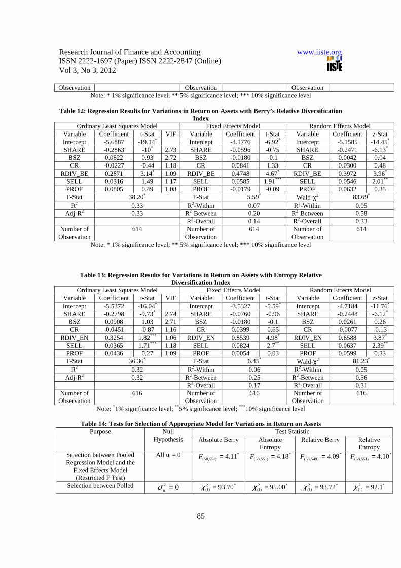
The results of the regression models on fluctuations in return on assets are presented in Table 10–13. It is observed that the F-statistics of all the pooled regression models and the fixed-effect models, and the Wald-χ2 statistic of all the random effect models are statistically significant for each of the alternative measures of operational diversification. Further, the value of adjusted R2 is reasonably high for each of these estimated models. This means that each of the estimated models is statistically significant with reasonably high explanatory power. Further, as in case of profitability, the restricted F-test, the Breusch and Pagan (1980) Lagrange Multiplier test, and the Hausman (1978) test suggest for using the regression results of the FEM for statistical inference and analysis of the individual coefficients (Table 14).

The VIF for the explanatory variables show that there is no severe multicollinearity problem in the estimated models. The test statistics for the individual coefficients are computed by using White’s (1980) heteroscedasticity corrected robust standard errors. It is observed that the coefficients of the extent of operational diversification and selling efforts (SELL) are statistically significant and positive. This means that the banks with greater extent of operational diversification or higher selling efforts suffer from the problem of greater fluctuations in return on assets. However, fluctuations in return on assets do not differ across the banks depending on their market share (SHARE), asset base (BSZ), current ratio (CR), or profitability level as the coefficient of these variables are not statistically significant.

From the regression results discussed above it is, therefore, clear that diversification of operations does not necessarily benefit a bank in terms of stability of its financial performance. Instead, under the competitive market conditions, financial performance may become more volatile, particularly when the extent of diversification exceeds a certain threshold. Such a direct relationship between operational diversification


78

and variations in financial performance is consistent with the findings of De Young and Roland (2001), Lepetit et al (2005), and Stiroh (2004a and 2004b). There may be a number of possible reasons for why operational diversification fails to bring in stability in financial performance of the banks. For example, it may be that the systematic risks have larger presence as compared to the unsystematic risks in Indian banking sector, and when it is so banks’ earning may become more volatile. As it is mentioned in the introductory section, operational diversification does not affect systematic risks, though it reduces unsystematic risks (Templeton and Severiens, 1992). Further, the impact of diversification on stability of financial performance may very well depend on the areas of diversification. This is so because entry into insurance sector may reduce the risks of bankruptcy, while that into securities/real estate sector can raise the same (Boyd and Graham, 1988; Lown et al., 2000).Over-diversification of operations may bring in inefficiency as well. It may also dilute the comparative advantage of managerial expertise (Klein and Saidenberg, 1998), and may make the financial performance unstable. Hence, while diversifying their operations, it is very important for the banks to determine the nature of risks, and the optimal level and the areas of diversification.

It is also found that the larger banks do not necessarily benefit from operational diversification. This may largely be due to their entry into the areas that are volatile in nature. Further, it is observed by Demsetz and Strahan (1997) that even through the large bank holding companies are better diversified than the small ones, their diversification fails to reduce risks due to lower capital ratios, larger commercial and industrial loan portfolios, and greater use of derivatives by large banks. In addition, the larger banks operating in India may also suffer when diversification exposes them to various new risks, but they do not have the necessary managerial expertise to manage these risks efficiently.

However, a direct relationship between selling efforts by a bank and fluctuations in its financial performance is surprising. It is generally expected that greater selling efforts would help a bank to stabilize its financial performance by restricting entry and creating image advantage in the sector. Contrary to this general proposition, the positive association between selling efforts and fluctuations in financial performance in the present context may be due to failure of the banks in creating effective strategic entry barriers or image advantage in the sector despite spending for these purposes. It may also be caused by regulatory interventions by the Reserve Bank of India in respect of rate of interest, CRR, etc. that reduce flexibility of the banks in making decisions on strategies. Further, research can be carried out to have deeper understanding in this regard.

5. Summary and Conclusions:

As a strategic response to enhanced competition in Indian banking sector due to reforms and subsequent entry of domestic and foreign private banks, many of the banks have followed the route of diversifying their operations to reduce the risks of business. In this perspective, the present paper is an attempt to examine the impact of this diversification strategy on fluctuations in financial performance of the banks. It is found that the banks with greater extent of operational diversification suffer from the problem of greater fluctuations in financial performance. Further, greater efforts by the banks towards creating entry barrier or image advantage also raise fluctuations in their financial performance. However, larger asset base does not necessarily help a bank to bring in stability in its financial performance.

The major findings of the present paper are, therefore, contradictory to the general proposition that greater extent of operational diversification or larger efforts towards creating strategic entry barriers and image advantage by the banks reduce fluctuations in their financial performance. This raises some important question: What is the nature of risks in Indian banking sector? To what extent should the banks diversify their operations and in which areas? Addressing these questions in future research is very important as over-diversification of operations or diversification into areas of noncore competencies not only affects stability of financial performance adversely, but may also create conflicts across the regulators for defining their jurisdiction of regulation, particularly when the areas of operations overlap. Further, in the absence of appropriate macroeconomic and regulatory structure, entry of foreign banks and emerging market


79

competition may increase the risks of crisis in Indian banking sector even if the banks diversify their operations.

References

Acharya, V.V., Hasan, I., & Saunders, A., (2006), “Should Banks be Diversified? Evidence from Individual Bank Loan Portfolios.” Journal of Business, 79(3), 1355-1412.

Ali-Yrkko, J. (2002),"Mergers and Acquisitions-Reasons and Results.” Discussion Paper Nr. 792, The Research Institute of the Finnish Economy, Helsinki

Arora, S. & Kaur, S. (2009), “Internal Determinants for Diversification in Banks in India an Empirical Analysis”, International Research Journal of Finance and Economics, 24, 177-185.

Bain, J. S. (1959), “Industrial Organization.” New York: Wiley

Berger, A.N., Hasan, I. & Zhou, M. (2010a), “The Effects of Focus versus Diversification on Bank Performance: Evidence from Chinese Banks.” Journal of Banking and Finance, 34(7), 1417-1435.

Berger, A. N., Hasan, I., Korhonen, I. & Zhou, M. (2010b), “Does Diversification Increase or Decrease Bank Risk and Performance? Evidence on Diversification and the Risk-Return Tradeoff in Banking”, BOFIT Discussion Paper No. 9, Bank of Finland.

Berry, C. H. (1971), “Corporate Growth and Industrial Diversification.” Journal of Law and Economics, 14(2), 371-383.

Berger, P.G., & Ofek, E. (1995), “Diversification’s Effect on Firm Value.” Journal of Financial Economics, 37(1), 39-65.

Bhaduri, S. (2010), “Non-Interest Diversification in Banking, the New Paradigm Shift after Liberalization and its Relevance as a Marketing Strategy”, retrieved from www.siescoms.edu as on September 20th, 2011.

Boyd, J.H., & Graham, S.L. (1988), “The Profitability and Risk Effects of Allowing Bank Holding Companies to Merge with Other Financial Firms: A Simulation Study.” Federal Reserve Bank of Minneapolis Quarterly Review, p.476-514.

Breusch, T., & Pagan, A. (1980), “The Lagrange Multiplier test and its Applications to Model Specification in Econometrics.” Review of Economic Studies, 47(1), 239-253.

Boot, A., & Schmeits, A. (2000), “Market Discipline and Incentive Problems in Conglomerate Firms with Applications to Banking.” Journal of Financial Intermediation, 9(3), 240–273.

Datta. I. M., & McLaughlin, R. (2007), “Global Diversification: New Evidence from Corporate Operating Performance.” Corporate Ownership and Control, 4, 228–250.

Denis, D.J., Denis, D.K., & Sarin, A. (1997), “Agency problems, equity ownership, and corporate diversification.” Journal of Finance, 52(1), 135–160.

De Young, R., Roland & K.P. (2001), “A risk-return framework for multiple-product industries”, Published in Emmanuel Acar (eds.), Value Added: Risk or Return? London: Financial Times/Prentice Hall. 193-198.

De Young, R. & Rice, T. (2004), “Non-interest Income and Financial Performance at U.S. Commercial Banks.” The Financial Review, 39(1), 456-478.

Drucker, S., & Puri, M.( 2009), “On loan sales, loan contracting, and lending relationships.” Review of Financial Studies, 22(7), p2835–2872.

Gujarati, D. N. & Sangeetha. (2009), “Basic Econometrics” Tata McGraw Hill, New Delhi

Hart, P. E. (1971), “Entropy and Other Measures of Concentration.” Journal of Royal Statistical Society, Series A, 134(1), 423-434.

Hausman, J. (1978), “Specification Tests in Econometrics” Econometrica, 46(6), 1251-72.


80

Jensen, M. (1986), “Agency Costs of Fee Cash Flow, Corporate Finance, and Takeovers.” American Economic Review, 76(2), 323-329.

Klein, P.,& Saidenberg, M. (1998), “Diversification, Organization, and Efficiency: Evidence from Bank Holding Companies.” Working Paper, Federal Reserve Bank of New York.

Kwan, S. (1998), “Risk and Return of Banks’ Section 20 Securities Affiliates.” FRBSF Economic Letter, 98-32.

Landi A. & Venturelli V. (2000), “The Diversification Strategy of European Banks: Determinants and Effects on Efficiency and Profitability.” retrieved from www.papers.ssrn.com.

Lepetit, L., Nysa, E., Rous, P. & Tarazi, A. (2005), “Bank Income Structure and Risk: An Empirical Analysis of European Banks.” Journal of Banking & Finance, 32(8), 1452–1467

Lown, C.S., Osier, C.L., Strahan, P.E., & Sufi, A. (2000), “The Changing Landscape of the Financial Service Industry: What Lies Ahead?.” Federal Reserve Bank of New York Economic Policy Review, 6, 39–54.

Mason, E. (1939), “Price and Production Policies of Large-Scale Enterprise.” American Economic Review, 29, 61-74.

Mishra, P. & Behera, B. (2007), “Instabilities in Market Concentration: An Empirical Investigation in Indian Manufacturing Sector.” Journal of Indian School of Political Economy, 19(3), 119-449.

Neuberger, D.(1997), "Structure, Conduct and Performance in Banking Markets." Thuenen-Series of Applied Economic Theory 12, University of Rostock, Institute of Economics, Germany.

Rose, P.S. (1989), “Diversification of the Banking Firm.” Financial Review, 24(2), 251-280.

Santomero A.W., & Chung E.J.(1992), “Evidence in Support of Broader Banking Powers.” Financial Markets, Institutions, and Instruments , 1(1), 1–69.

Saunders, A., Strock, E., & Travlos, N.G. (1990), “Ownership Structure, Deregulation, and Bank Risk Taking.” Journal of Finance, 45(2),643–654.

Servaes, H. (1996), “The Value of Diversification during the Conglomerate Merger Wave.” Journal of Finance, 51(4),1201-1225.

Steinherr, A. & Huveneers Ch. (1990), “Universal Banks: The Prototype of Successful Banks in the Integrated European Market: A View Inspired by German Experience.” Research Report No. 2, Centre for European Policy Studies (CEPS), Brussels.

Stiroh, K.J.( 2004a), “Diversification in Banking: Is Non-Interest Income the Answer?” Journal of Money, Credit and Banking, 36(154),853-82.

Stiroh, K.J.( 2004b), “Diversification in Banking: Is Noninterest Income the Answer?” Journal of Money, Credit, and Banking, 36, No.5, p.853-882.

Stiroh, K.J., & Rumble A. (2006), “The Dark Side of Diversification: The Case of U.S. Financial Holding Companies,” Journal of Banking and Finance, 30(8), 2131-2161.

Templeton, W.K., & Severiens, J.T. (1992), “The Effects of Non-Bank Diversification on Bank Holding Company Risk.” Quarterly Journal of Business and Economics, 31(1),3-17.

Xu, J. (1996), “An Empirical Estimation of the Portfolio Diversification Hypothesis; The Case of Canadian International Banking.” The Canadian Journal of Economics, 29, special issue: Part1,S192-S197.

White, H. (1980), “A Heteroscedasticity Consistent Covariance Matrix Estimator and a Direct Test of Heteroscedasticity.” Econometrica, 48(4),817-818.

Winton, A. (1999), “Don’t Put all your Eggs in one Basket? Diversification and Specialization in Lending.” Working Paper, University of Minnesota.


81

Table1: ANOVA for Operational Diversification of Banks

Index Nature of Ownership Variations across Banks Variations over Time

ADIV_BE

Public F(24,288)=25.15* F(12,288)=23.45 *

Private Domestic F(11,132)=8.13* F(12,132)=2.91*

Private Foreign F(18,216)=8.79 * F(12,216)=15.60*

Total F(57,684)=11.32* F(12,684)=22.95*

ADIV_EN

Public F(24,288)=18.95 * F(12,288)=30.67 *


Private Foreign F(18,216)=5.57* F(12,216)=14.77*

Total F(57,684)=8.78* F(12,684)=29.62*

RDIV_BE

Public F(24,288)=25.59* F(12,288)=29.83*



Total F(57,684)=12.84* F(12,684)=33.41*

RDIV_EN

Public F(24,288)=18.58* F(12,288)=14.56*

Private Domestic F(11,132)=2.44** F(12,132)=1.47


Total F(57,684)=8.38* F(12,684)=8.74*

Note: Figures in the parentheses of the F statistic indicate respective degrees of freedom *statistically significant at 1%

Table 2: ANOVA for Fluctuations of Financial Performance Index Nature of Ownership Variations across Banks Variations over Time

VPROF

Public F(24,288)=9.41* F(12,288)=11.90*

Private Domestic F(11,132)=2.22** F(12,132)=10.38*

Private Foreign F(18,216)=11.70* F(12,216)=1.42

Total F(57,684)=11.63* F(12,684)=12.17*

VROA

Public F(24,288)=11.82* F(12,288)=13.50*


Private Foreign F(18,216)=8.99* F(12,216)=0.68

Total F(57,684)=12.49* F(12,684)=3.17*

Note: Figures in the parentheses of the F statistic indicate respective degrees of freedom *statistically significant at 1%


82

Table 3: Summary Statistics of the Variables Used in the Regression Models

Variable No. of Observation

Average Standard Deviation

Maximum Minimum

VPROF 708 -2.84 0.837 -5.076 -0.177

VROA 708 -4.61 0.780 -1.794 -8.043

SHARE 708 -5.20 1.647 -10.189 -1.465

BSZ 705 1.53 0.508 -2.748 2.200

CR 708 1.18 0.634 -0.769 4.614

SELL 620 -6.47 1.416 -10.123 -2.508

PROF 705 -0.46 0.245 -2.885 -0.062

ROA 708 -4.61 0.780 -8.043 -1.794

ADIV_BE 708 -0.64 0.237 -2.186 -0.238

ADIV_EN 708 -0.61 0.238 -2.139 -0.392

RDIV_BE 700 -1.06 0.511 -7.202 -0.468

RDIV_EN 708 -1.17 0.201 -2.466 -0.540

Table 4: Regression Results for Variations in Profitability with Berry’s Absolute Diversification Index

Ordinary Least Squares Model Fixed Effects Model Random Effects Model Variable Coefficient t-Stat VIF Variable Coefficient t-Stat Variable Coefficient z-Stat Intercept -4.4885 -19.32* Intercept -3.3041 -4.60* Intercept -4.1007 -11.77* SHARE -0.2553 -10.95* 2.72 SHARE -0.1985 -2.11** SHARE -0.2596 -7.34*

BSZ 0.0703 1.25 2.71 BSZ 0.1028 0.53 BSZ 0.0995 1.13 CR -0.0047 -0.09 1.18 CR 0.1895 2.31** CR 0.0788 1.19

ADIV_BE 0.4389 2.95* 1.10 ADIV_BE 0.6510 4.17* ADIV_BE 0.5550 3.83* SELL -0.0060 -0.28 1.18 SELL 0.1455 4.22* SELL 0.0582 2.13** PROF -0.9027 -4.69* 1.10 PROF -0.7675 -3.14* PROF -0.7996 -3.64* F-Stat 44.04* F-Stat 10.58* Wald-χ2 125.31*

R2 0.36 R2-Within 0.15 R2-Within 0.14 Adj-R2 0.35 R2-Between 0.37 R2-Between 0.57

R2-Overall 0.26 R2-Overall 0.34 Number of Observatio

n

616 Number of Observation


616

Note: * 1% significance level; ** 5% significance level Table 5: Regression Results for Variations in Profitability with Entropy Absolute Diversification

Index Ordinary Least Squares Model Fixed Effects Model Random Effects Model

Variable Coefficient

t-Stat VIF Variable Coefficient t-Stat Variable Coefficient z-Stat

Intercept -4.6631 -19.58* Intercept -3.5934 -5.04* Intercept -4.3679 -13.22* SHARE -0.2573 -10.80* 2.73 SHARE -0.2114 -2.21** SHARE -0.2665 -7.90**

BSZ 0.0723 1.28 2.72 BSZ 0.1347 0.72 BSZ 0.1071 1.29


83

CR -0.0207 -0.40 1.18 CR 0.1780 2.15** CR 0.0529 0.83 ADIV_EN 0.1426 0.89 1.08 ADIV_EN 0.3453 2.02*** ADIV_EN 0.2553 1.61*

SELL -0.0014 -0.06 1.16 SELL 0.1510 4.43* SELL 0.0542 2.03 PROF -0.9674 -5.03* 1.06 PROF -0.8339 -3.32* PROF -0.8762 -3.99* F-Stat 42.88* F-Stat 8.07* Wald-χ2 124.44*


R2-Overall 0.25 R2-Overall 0.34 Number of Observation



616

Note: * 1% significance level; ** 5% significance level; *** 10% significance level

Table 6: Regression Results for Variations in Profitability with Berry’s Relative Diversification Index

Ordinary Least Squares Model Fixed Effects Model Random Effects Model Variable Coefficient t-Stat VIF Variable Coefficient t-Stat Variable Coefficient z-Stat Intercept -4.5658 -19.87* Intercept -3.4278 -4.76* Intercept -4.2099 -12.21* SHARE -0.2582 -11.04 2.73 SHARE -0.1948 -2.06** SHARE -0.2635 -7.51*


RDIV_BE 0.1995 2.39** 1.09 RDIV_BE 0.3164 3.23* RDIV_BE 0.2629 2.97* SELL -0.0054 -0.25 1.17 SELL 0.1409 4.04* SELL 0.0566 2.06** PROF -0.9187 -4.79* 1.08 PROF -0.7897 -3.22* PROF -0.8172 -3.73* F-Stat 43.65* F-Stat 8.38* Wald-χ2 118.73*





614

Note: * 1% significance level; ** 5% significance level; *** 10% significance level Table 7: Regression Result for Variations in Profitability s with Entropy Relative Diversification


Variable Coefficient t-Stat VIF Variable Coefficient t-Stat Variable Coefficient z-Stat Intercept -4.3477 -14.13* Intercept -2.7306 -3.74* Intercept -3.7944 -9.64* SHARE -0.2527 -10.49* 2.74 SHARE -0.1999 -2.18** SHARE -0.2570 -7.31*


RDIV_EN 0.3208 1.92*** 1.09 RDIV_EN 0.7396 4.80* RDIV_EN 0.5334 3.47* SELL -0.0033 -0.15 1.16 SELL 0.1544 4.70* SELL 0.0573 2.16** PROF -0.9317 -4.84* 1.06 PROF -0.7598 -3.08* PROF -0.8161 -3.74* F-Stat 45.0* F-Stat 11.88* Wald-χ2 138.38*





616

Note: * 1% significance level; ** 5% significance level; *** 10% significance level Table 8: Tests for Selection of Appropriate Model for Variations in Profitability

Purpose Null

Hypothesis

Test Statistics Absolute

Berry Absolute Entropy

Relative Berry Relative Entropy


84

Selection between Polled Regression Model and Fixed

Effects Model (Restricted F Test)

All u i = 0 *)551,58( 69.3====F

*)551,58( 62.3====F

*)549,58( 67.3====F

*)551,58( 84.3====F

Selection between Polled Regression Model and Random Effects Model (Breusch-Pagan

Lagrange Multiplier Test)

02 =uσ *2)1( 12.60====χ *2

)1( 17.57====χ *2)1( 08.61====χ *2

)1( 01.62====χ

Selection between Fixed Effects Model and Random Effects Model

(Hausman Test)

Difference in coefficients is not systematic

*2)6( 63.36====χ *2

)6( 24.27====χ *2)6( 33.32====χ **2

)6( 11.16====χ

Note: * 1% significance level

Table 10: Regression Results for Variations in Return on Assets with Berry’s Absolute Diversification Index

Ordinary Least Squares Model Fixed Effects Model Random Effects Model Variable Coefficient t-Stat VIF Variable Coefficient t-Stat Variable Coefficient z-Stat Intercept -5.5823 -18.72* Intercept -4.0107 -6.71* Intercept -5.0014 -13.85* SHARE -0.2820 -9.84* 2.72 SHARE -0.0673 -0.85 SHARE -0.2415 -5.95*

BSZ 0.0847 0.96 2.71 BSZ -0.0360 -0.21 BSZ 0.0041 0.04 CR -0.0190 -0.36 1.18 CR 0.0779 1.24 CR 0.0290 0.46

ADIV_BE 0.6211 3.87* 1.1 ADIV_BE 0.9556 5.46* ADIV_BE 0.8250 4.99* SELL 0.0309 1.44 1.18 SELL 0.0666 2.17** SELL 0.0569 2.09 PROF 0.1009 0.61 1.1 PROF 0.0156 0.08 PROF 0.0883 0.48 F-Stat 38.36* F-Stat 7.22* Wald-χ2 90.46*





616

Note: * 1% significance level; ** 5% significance level Table 11: Regression Results for Variations in Return on Assets with Entropy Absolute

Diversification Index Ordinary Least Squares Model Fixed Effects Model Random Effects Model

Variable Coefficient t-Stat VIF Variable Coefficient t-Stat Variable Coefficient z-Stat Intercept -5.7352 -19.15* Intercept -4.1608 -6.94* Intercept -5.2040 -14.62* SHARE -0.2858 -9.76* 2.73 SHARE -0.0775 -1 SHARE -0.2514 -6.24*

BSZ 0.0796 0.9 2.72 BSZ -0.0802 -0.44 BSZ -0.0019 -0.02 CR -0.0399 -0.78 1.16 CR 0.0786 1.29 CR 0.0144 0.24

ADIV_EN 0.3965 2.4** 1.08 ADIV_EN 0.8251 5.11* ADIV_EN 0.6600 4.2* SELL 0.0338 1.58 1.18 SELL 0.0639 2.08** SELL 0.0545 2.02** PROF 0.0163 0.1 1.06 PROF -0.0871 -0.45 PROF -0.0074 -0.04 F-Stat 36.69* F-Stat 6.81* Wald-χ2 82.76*


R2-Overall 0.18 R2-Overall 0.32 Number of 616 Number of 616 Number of 616


85

Observation Observation Observation Note: * 1% significance level; ** 5% significance level; *** 10% significance level

Table 12: Regression Results for Variations in Return on Assets with Berry’s Relative Diversification


Variable Coefficient t-Stat VIF Variable Coefficient t-Stat Variable Coefficient z-Stat Intercept -5.6887 -19.14* Intercept -4.1776 -6.92* Intercept -5.1585 -14.45* SHARE -0.2863 -10* 2.73 SHARE -0.0596 -0.75 SHARE -0.2471 -6.13*

BSZ 0.0822 0.93 2.72 BSZ -0.0180 -0.1 BSZ 0.0042 0.04 CR -0.0227 -0.44 1.18 CR 0.0841 1.33 CR 0.0300 0.48

RDIV_BE 0.2871 3.14* 1.09 RDIV_BE 0.4748 4.67* RDIV_BE 0.3972 3.96* SELL 0.0316 1.49 1.17 SELL 0.0585 1.91*** SELL 0.0546 2.01** PROF 0.0805 0.49 1.08 PROF -0.0179 -0.09 PROF 0.0632 0.35 F-Stat 38.20* F-Stat 5.59* Wald-χ2 83.69*





614

Note: * 1% significance level; ** 5% significance level; *** 10% significance level

Table 13: Regression Results for Variations in Return on Assets with Entropy Relative Diversification Index

Ordinary Least Squares Model Fixed Effects Model Random Effects Model Variable Coefficient t-Stat VIF Variable Coefficient t-Stat Variable Coefficient z-Stat Intercept -5.5372 -16.04* Intercept -3.5327 -5.59* Intercept -4.7184 -11.76* SHARE -0.2798 -9.73* 2.74 SHARE -0.0760 -0.96 SHARE -0.2448 -6.12*

BSZ 0.0908 1.03 2.71 BSZ -0.0180 -0.1 BSZ 0.0261 0.26 CR -0.0451 -0.87 1.16 CR 0.0399 0.65 CR -0.0077 -0.13

RDIV_EN 0.3254 1.82*** 1.06 RDIV_EN 0.8539 4.98* RDIV_EN 0.6588 3.87* SELL 0.0365 1.71*** 1.18 SELL 0.0824 2.7** SELL 0.0637 2.39** PROF 0.0436 0.27 1.09 PROF 0.0054 0.03 PROF 0.0599 0.33 F-Stat 36.36* F-Stat 6.45* Wald-χ2 81.23*





616

Note: *1% significance level; ** 5% significance level; *** 10% significance level

Table 14: Tests for Selection of Appropriate Model for Variations in Return on Assets Purpose Null

Hypothesis Test Statistic

Absolute Berry Absolute Entropy

Relative Berry Relative Entropy

Selection between Pooled Regression Model and the

Fixed Effects Model (Restricted F Test)

All u i = 0 *)551,58( 11.4=F *

)551,58( 18.4=F

*)549,58( 09.4=F

*)551,58( 10.4=F

Selection between Polled 02 =uσ *2)1( 70.93=χ *2

)1( 00.95=χ *2)1( 72.93=χ *2

)1( 1.92=χ


86

Regression Model and Random Effects Model

(Breusch-Pagan Lagrange Multiplier Test)

Selection between Fixed Effects Model and Random

Effects Model (Hausman Test)

Difference in coefficients is not systematic

*2)6( 83.20=χ *2

)6( 23.358=χ *2)6( 23.20=χ *2

)6( 73.1349=χ

Note: * 1% significance level

Appendix I

Measurement of Variables As mentioned earlier, in the present paper, the specified regression equation is estimated by using bank level data collected from the PROWESS database of CMIE. In order to control for the measurement errors, if any, and also to control for the process of adjustment, three years’ moving average is taken for each of the independent variables. Accordingly, all the independent variables are measured as simple average of previous three years with the year under reference being the starting year. Such a lag structure is expected to control the potential simultaneity in the envisaged relationships.

Fluctuations in Performance (VPER)

The risk of operation of a bank is measured in terms of standard deviation of its financial performance over a period of five years with the year under reference being at the centre. Two alternative indicators of financial performance, viz., profitability (PROF) and returns on assets (ROA) are used to substantiate the findings. Hence, the variations in profitability (VPROF) are measured by using the following formula:

),,,,( 2,1,1,2, ++−−= titiittitiit PROFPROFPROFPROFPROFVPROF σ

Similarly, the variations in return on assets (VROA) are measured as the following:

),,,,( 2,1,1,2, ++−−= titiittitiit ROAROAROAROAROAVROA σ

Market Share (SHR)

Market share of bank i in year t (SHRit) is measured as the ratio of its income (Ii) to total income of all the banks in the sector, i.e.,

∑∑∑=

−

−

=−

−

=

++=n

iti

ti

n

iti

ti

n

iit

itit

I

I

I

I

I

ISHR

12,

2,

11,

1,

1

where, n stands for income of banks in the industry.

Bank Size (BSZ)

Size or asset base of a bank in year t (BSZit) is measured as the natural logarithm of its gross fixed assets (GFA), i.e.,


87

3

)ln()ln()ln( 2,1, −− ++= titiit

it

GFAGFAGFABSZ

Performance (PER)

Like fluctuations in financial performance, for its level also two alternative indicators are used, viz., profitability (PROF) and the returns on assets (ROA). Profitability of bank i in year t (PROFit) is measured as the ratio of profit before interest and tax (PBIT) of the bank to its total income (Ii), i.e.,

2,

2,

1,

1,

−−−−

−−−−

−−−−

−−−− ++++++++====ti

ti

ti

ti

it

itit I

PBIT

I

PBIT

I

PBITPROF

Similarly, the returns on assets of bank i in year t (ROAit) is measured as the ratio of profit before interest and tax (PBIT) of the bank to its gross fixed assets (GFAi), i.e.,

2,

2,

1,

1,

−−−−

−−−−

−−−−

−−−− ++++++++====ti

ti

ti

ti

it

itit GFA

PBIT

GFA

PBIT

GFA

PBITROA

Current Ratio (CR)

The current ratio of bank i in year t (CRit) is measured as the ratio of its current assets (CA) to current liabilities (CL), i.e.,

2,

2,

1,

1,

−−−−

−−−−

−−−−

−−−− ++++++++====ti

ti

ti

ti

it

itit CL

CA

CL

CA

CL

CACR

Diversification

As it is mentioned earlier, the present paper uses two different measures of diversification, viz., the Berry’s index, and the entropy index to substantiate the findings. Further, in both the cases, the indices are used to measure degree of diversification in absolute as well as in relative sense.

Absolute Diversification – Berry’s Index:

3

____ 2,1, −−−−−−−− ++++++++

==== titiitit

BEADIVBEADIVBEADIVBEADIV

Absolute Diversification – Entropy Index

3

____ 2,1, −−−−−−−− ++++++++

==== titiitit

ENADIVENADIVENADIVENADIV

Relative Diversification – Berry’s Index

3

____ 2,1, −−−−−−−− ++++++++

==== titiitit

BERDIVBERDIVBERDIVBERDIV

Relative Diversification – Entropy Index

3

____ 2,1, −−−−−−−− ++++++++

==== titiitit

ENRDIVENRDIVENRDIVENRDIV

This academic article was published by The International Institute for Science,

Technology and Education (IISTE). The IISTE is a pioneer in the Open Access

Publishing service based in the U.S. and Europe. The aim of the institute is

Accelerating Global Knowledge Sharing.

More information about the publisher can be found in the IISTE’s homepage:

http://www.iiste.org

The IISTE is currently hosting more than 30 peer-reviewed academic journals and

collaborating with academic institutions around the world. Prospective authors of

IISTE journals can find the submission instruction on the following page:

http://www.iiste.org/Journals/

The IISTE editorial team promises to the review and publish all the qualified

submissions in a fast manner. All the journals articles are available online to the

readers all over the world without financial, legal, or technical barriers other than

those inseparable from gaining access to the internet itself. Printed version of the

journals is also available upon request of readers and authors.

IISTE Knowledge Sharing Partners

EBSCO, Index Copernicus, Ulrich's Periodicals Directory, JournalTOCS, PKP Open

Archives Harvester, Bielefeld Academic Search Engine, Elektronische

Zeitschriftenbibliothek EZB, Open J-Gate, OCLC WorldCat, Universe Digtial

Library , NewJour, Google Scholar

http://www.iiste.org/

http://www.iiste.org/Journals/

operational diversification and stability of financial

Documents