diversification and financial stability - chair of systems design

Diversification and Financial Stability

Paolo Tasca, Stefano Battiston

CCSS Working Paper Series

CCSS-11-001

CCSS, the Competence Center Coping with Crises in Complex Socio-Economic Systems, wasestablished at ETH Zurich (Switzerland) in September 2008. By means of theoretical and empiricalanalysis, CCSS aims at understanding the causes of and cures to crises in selected problem ar-eas, for example in financial markets, in societal infrastructure, or crises involving political violence.

More information can be found at: http://www.ccss.ethz.ch/.

CCSS-11-001


Paolo Tasca, Stefano Battiston

Abstract

The recent credit crisis of 2007/08 has raised a debate about the so-called knife-edge properties offinancial markets. The paper contributes to the debate shedding light on the controversial relation be-tween risk-diversification and financial stability. We model a financial network where assets held byborrowers to meet their obligations, include claims against other borrowers and securities exogenous tothe network. The balance-sheet approach is conjugated with a stochastic setting and by a mean-fieldapproximation the law of motion of the system’s fragility is derived. We show that diversification hasan ambiguous effect and beyond a certain levels elicits financial instability. Moreover, we find that risk-sharing restrictions create a socially preferable outcome. Our findings have significant implications forfuture policy recommendation.

Keywords: Systemic Risk, Financial Crisis, Diversification, Default Probability

Classifications: JEL Codes: G01, G11, G18, G2, G32, G33

URL: http://web.sg.ethz.ch/wps/CCSS-11-001

Notes and Comments: Status: Submitted

CCSS Working Paper Series

Paolo Tasca(1,2), Stefano Battiston(1):Diversification and Financial Stability


Paolo Tasca(1,2), Stefano Battiston(1)

(1) Chair of Systems Design, ETH Zurich, Switzerland, (2) Ca’ Foscari Univ. Venice, Italy

Abstract

The recent credit crisis of 2007/08 has raised a debate about the so-called knife-edge propertiesof financial markets. The paper contributes to the debate shedding light on the controversial rela-tion between risk-diversification and financial stability. We model a financial network where assetsheld by borrowers to meet their obligations, include claims against other borrowers and securitiesexogenous to the network. The balance-sheet approach is conjugated with a stochastic setting andby a mean-field approximation the law of motion of the system’s fragility is derived. We show thatdiversification has an ambiguous effect and beyond a certain levels elicits financial instability. More-over, we find that risk-sharing restrictions create a socially preferable outcome. Our findings havesignificant implications for future policy recommendation.

JEL Code: G01, G11, G18, G2, G32, G33Keywords: Systemic Risk, Financial Crisis, Diversification, Default Probability.

1 Introduction

The recent financial crisis is attracting increasing attention on the knife-edge properties of the financialsystem and its optimal architecture (see e.g., Gai and Kapadia, 2007; Haldane and May, 2011; Nieret al., 2007). In a nutshell, this means that within a certain range, financial interconnections serve asshock-absorber (i.e., connectivity engenders robustness and risk-sharing prevails). But beyond the tippingpoint, interconnections serve as shock-amplifier (i.e., connectivity engenders fragility and risk-spreadingprevails). It has been argued that these knife-edge dynamics, can essentially be explained by two structuralfeatures over of the financial network. They are complexity on the one hand, and homogeneity on theother (Haldane, 2009). The paper contributes to this discussion by shedding light on the relation betweendiversification and financial stability. It investigates how diversification affects the probability of failure,both from an individual and a systemic perspective, when financial institutions are (1) interlinked at

We are grateful to Rahul Kaushik, Moritz Muller, Paolo Pellizzari, Frank Schweitzer, Claudio J. Tessone and participantsat various seminars and conferences where a preliminary version of this paper was presented. The authors acknowledge thefinancial support from: the ETH Competence Center “Coping with Crises in Complex Socio-Economic Systems” CHIRP 1(grant no. CH1-01-08-2), the European Commission FET Open Project “FOC” (grant no. 255987), and the Swiss NationalScience Foundation project “OTC Derivatives and Systemic Risk in Financial Networks” (grant no. CR12I1-127000/1).

Address correspondence to Paolo Tasca, Chair of Systems Design, ETH, Zurich, Kreuzplatz 5 8032 Zurich; e-mail:[email protected].

1/25


the balance-sheet level in a network of obligations and (2) invest in activities external to the financialnetwork. Until recently, many theoretical models of finance pointed towards the stabilizing effects ofa diversified (i.e., dense) financial network, (Allen and Gale, 2001). Some recent work has started tochallenge this view, investigating conditions under which diversification may have ambiguous effects;e.g., Battiston et al. (2009); Brock et al. (2009); Ibragimov et al. (2011); Ibragimov and Walden (2007);Stiglitz (2010); Wagner (2009).

In a similar spirit as Shin (2008, 2009), we model a financial network composed of leveraged risk-aversefinancial institutions (hereafter “banks”), which invest in two classes of assets. The first class consistsof obligations issued by other banks in the network. 1 The second class represents assets external tothe financial network, which may include securities on, e.g., real-estate and other real-economy relatedactivities, or loans to firms and households (hereafter “external assets”). We assume that external assetsmay be in a downtrend (hereafter, downturn) with probability p, or in an uptrend (hereafter, upturn), withprobability 1 − p. In this uncertain world, it is assumed that banks have an incentive to diversify acrossexternal assets.1 Precisely, the strategy consists of choosing an optimal portfolio that maximizes theirexpected Mean-Variance (MV) utility function. For the sake of simplicity it is assumed that banks adopta “naive” strategy which involves holding an equally weighted portfolio of external assets. Two importantassumptions of the model are as follows: first, the up(down)turn is persistent i.e., approximately constantduring a given period ∆t; second, due to information-gathering and transaction costs, the diversificationstrategy is assumed to be static for a given period ∆t.2 These two assumptions imply that, based on theexpectation about the future trend of external assets, each bank sets up a diversified portfolio which willbe held for a finite arbitrary interval ∆t.

A first contribution of the paper is to show that banks’ default probability increases with diversification incase of a downturn and decreases in case of an upturn. There is a simple intuition for this effect in termsof the Sharpe ratio which allows to compare different investment returns per unit of risk. When assetshave positive expected cash-flows the Sharpe ratio is positive as well. Then it is desirable to combinethem in a well diversified portfolio since diversification lowers portfolio’s volatility and in doing so,increases its Sharpe ratio. In contrast, when assets have negative expected cash-flows, the Sharpe ratiois negative. Then, a well diversified portfolio is no longer desirable. From the first finding, it followsthat the gap between expected MV utility in upturn, w.r.t. expected MV utility in downturn, increases

1 Although in our simplified economy, the securities in this class are priced depending on the financial health of the obligors,in reality, the debt-claim structure of the financial system is much more intricate. To better understand this view, we need toachieve a clear understanding of the building blocks of financial system, mostly in the presence of amplification mechanismstemming from leverage and other factors, (see Trichet, 2009). The banks’ asset values depend on the payoffs received from theclaims on other banks in which they have invested. But the value of these issuing banks depends, in turn, on the financial healthof yet other banks in the system. Moreover, linkages between banks can be cyclical. See Eisenberg and Noe (2001).

1 Generally, this practice is desirable since it allows banks to promise investors a lower repayment or increase the amountof debts. See Allen et al. (2010).

2In the real-world, portfolio adjustments are costly. In particular, the revision costs sometimes could be greater than theincrease of the expected rate of return of the revised portfolio. So, portfolio revision is not always convenient.

2/25


with diversification. Thus, diversification generates and amplifies the knife-edge property of the financialnetwork. Moreover, for a given level of diversification, the gap in utility increases with the magnitude ofthe trend. In other words, we show that diversification is a double-edged strategy, in the words of Haldane(2009).

In the hypotheses that (1) banks’ portfolios of external assets do not overlap (i.e., they are not positivelycorrelated) and (2) banks are not interconnected (i.e., they do not invest in other banks’ obligations), eachbank’s default is an independent event. The model relaxes both those hypotheses such that the default ofa single bank is very likely to have a systemic impact. Similarly to Acharya (2009), the relaxation of thefirst hypothesis implies that the systemic failure is the joint failure arising from the correlation of returnson asset-side of banks’ balance-sheet. Whereas, resembling Ibragimov et al. (2011), by relaxing the sec-ond hypothesis, the systemic risk is introduced when banks with limited liability become interdependentby taking position in other banks’ obligations. To summarize, in this setting, we find that diversification,even though desirable in upturn periods, tends to induce a systemic failure in downturn periods. Thiseffect is in line with the robust-yet-fragile property of “connected” networks (see e.g., May et al., 2008).

On the basis of the first contribution, the paper shows that by assigning a probability p to the downturnevent and 1 − p to the upturn event, diversification displays a tradeoff w.r.t. the bank’s utility. Thismeans that, the expected MV utility exhibits a maximum which corresponds to an intermediate level ofdiversification. Such a level depends on the probability p of downturn, on the magnitude of the expectedprofit (loss) and on the values of the other parameters of the model.

In the presence of limited liability, the expected loss of an individual bank is bounded. In contrast, atthe system level, either due to direct or indirect exposures, the externalities associated with the failureof interconnected institutions, amplify the expected losses. These externalities reflect the “incrementalcosts” due to a system collapse which are ultimately borne by taxpayers. In other words, the cost ofrecovery from a systemic crisis, grows with the number of defaults. Under this condition, we find thatthe optimal level of diversification for the regulator is always smaller than the one desirable at individuallevel. This leads us to another finding. Individual banks’ incentives favor a financial network that is over-diversified in external assets w.r.t. to the level of diversification that is socially desirable. Therefore, ouranalysis has some implications for risk management and policies to mitigate systemic risk.

The paper is organized as follows. In Section 2 we introduce the model. Section 3 derives the finan-cial fragility under the mean-field approach. Section 4 moves from the financial fragility to the defaultprobability and the optimal diversification policy. Section 5 investigates the dichotomy between privateincentives of diversification and its social effects. Section 6 concludes and considers some extensions.

3/25


2 Model

In a similar spirit as Shin H.S.Shin (2008, 2009), we model a system of n financial risk-averse leveragedinstitutions (“banks”). The balance-sheet identity conceives the equilibrium between asset an liabilityside, which for the representative bank-i ∈ 1, ..., n, is

ai = pi + ei , (1)

where a := (a1, ..., an)T is the column vector of market values of the banks’ assets; p := ( p1, ..., pn)T isthe column vector of the book-face values of the banks’ obligations (e.g., zero-coupon bonds); 3 e :=(e1, ..., en)T is the column vector of equity values. Notably, each bank asset-side is composed by twoinvestment classes: (i) n − 1 obligations, each issued by one of the other banks in the system, and (ii)m exogenous investment opportunities non related to the financial sector (external assets). Then, theasset-side in (1) becomes

ai :=m∑j

Zi jy j +

n∑j

Wi j p j , (2)

where

p j := p j/(1 + r j)−t (3)

is the market value of debt issued by bank- j, defined as the discounted value of future payoffs; y :=(y1, ..., ym)T is the column vector of external investments; Z := [zi j]n×m is the n × m weighting matrix ofexternal investments where each entry zi, j is the proportion of activity- j held by bank-i; W := [wi j]n×n isthe n × n adjacency matrix where each entry wi j is the proportion of bank- j debt held by bank-i; r j : isthe rate of return used to discount the debt-face value of the obligor- j. In brief, the bank-i manages thefollowing balance-sheet

Assets Liabilities∑mj Zi jy j pi∑nj Wi j p j ei

Kept the adjacency matrix W := [wi j]n×n of claims and obligation among banks as given, the objectivefunction of risk-averse banks, is to increase their asset value per unit of risk. This goal can be achievedthrough the following management strategy.

Definition 2.1. Management Strategy In a one period capital-allocation problem, banks strategy con-sists in wealth diversification among the investment opportunities offered by the non-financial sectorrepresented by the adjacency matrix Z := [Zi j]n×m.

3In particular, pi is the value of the payment at maturity that each obligor-i promised to the lenders. For all the banks in thesystem, the equation indirectly assumes only one issue of bonds with the same maturity date t.

4/25


External assets include e.g., activities related to the real-economy, loans to firms and households, etc.,and each of them it is assumed to generates a log-normal cash flows process

dlog(Y j)(t) := dy j(t) = µ jdt + σ jdB j(t) ∀ j = 1, ...,m , (4)

where B j(t) is a standard Brownian motion defined on a complete filtered probability space(Ω;F ; Ft;P), with Ft = σyB(s) : s ≤ t, µ j is the instantaneous risk-adjusted expected growth rate,σ j > 0 is the volatility of the growth rate. We assume correlation across processes d(Bi, B j) = ρi j andi.i.d. returns for each of them. The processes in (4) have the relevant property that they preclude instan-taneous external assets’ distributions from becoming negative at any time t ≥ 0 and are therefore aneconomically reasonable assumption.

The results in the next Sections hold under the following main assumption of the model.

Assumption 2.1. (i) There exists a frictionless market where all debt-securities have the same maturitydate and seniority; (ii) Divisibility and Not-short selling constraint. All the securities are marketable,perfectly divisible and can be held only in positive quantities; (iii) Price Taking Assumption. Securitiesprices are beyond the influence of investors; (iv) Only expected returns and variances matter. Quadraticutility or normally distributed returns; (v) Not-paying dividend-coupon assumption. The return on anysecurity is simply the change in its market price during the holding period; (vi) Homogeneous expecta-tions

2.1 Leverage and Balance-Sheet Management

Given the vector φ ∈ Rn×1 of debt-asset ratios, a standard accounting approach is to consider φi ∈ [0, 1]as the bank’s i leverage, such that

φi = pi/ai

= pi/

m∑j

Zi jy j +

n∑j

Wi j p j

. (5)

The balance-sheet equilibrium between sources of finance and investments cash-flows is a precondition4

to solvency. In fact, the solvency of a bank is indicated by the positive net worth as measured by dif-ference between assets and liabilities (excluding capital and reserves). Then the problem of a failingbank normally emerges through illiquidity. In this perspective, the debt-asset ratio is a leverage indicatorresuming the potential insolvency of a bank due to a fragile capital structure.

Definition 2.2. Bank Fragility. The debt-asset ratio φ is a leverage index that maps the bank’s fragilitybetween zero and one.

4Necessary but not sufficient.

5/25


A leverage φ which tends to one is symptomatic of a very fragile bank that is prone to be highly sensitiveto external shocks which may force the bank towards a bankruptcy regime. On the other hand, a leverageφ close to zero describes a bank with a solid balance-sheet equilibrium between internal and externalsources of finance.

In line with a large body of theoretical and empirical literature, the rate of return on future paymentsdepends upon the payor’s credit-worthiness (e.g. measured by its leverage), the contractual features (e.g.,time to maturity) and the market factors. In our simplified economy, the only two factors explaining theinternal rate of return, are the risk-free rate r f and the indicator of fragility φ such that, for each obligor- jthe following equation holds true

r j := r f + βφ j . (6)

The risk-free rate5 is fixed over time and is in the common knowledge of every institution: E(r f ) = r f

and Var(r f ) = 0. The parameter β in R ∈ [0, 1] can be interpreted as the responsiveness of the rate ofreturn to a firm’s financial condition. Finally, φ j is defined as in (5).6

An extensive form of the balance-sheet management of the bank can be now derived substituting (6) into(3)7 and then (3)8 into (5)

φi = pi/

m∑j

Zi jy j +

n∑j

Wi j p j/(1 + r f + (βφ j

) . (7)

Eq. (7) shows a non-linear dependence of the fragility φi related to the representative bank-i, with thefragilities φ j=1,...,n of the j-banks, obligors of i. The following feature of our model is then immediate.

Lemma 2.3. At a macro level, it can be shown that the fragility of the banking system is the positive rootof a system of parabolic expressions in φ.

Proof. See Appendix A.

Since (7) is too complex to analyze directly under arbitrary network structures, we follow the usualtechnique of analyzing a mean-field approximation to the given expression (see e.g., Vega-Redondo,2007).

5The risk-free rate is paid by an asset without any default, timing or exchange rate risk; as such, it is a non-observabletheoretical construct. It is usually measured by the rates of return on government securities, which have the lowest risk, in anyparticular currency.

6With the opportune swap between sub-index j and i.7This substitution makes evident that pi is an inverse function of φi. Higher leverage implies a lower market price of the

claims and a greater internal rate of return.8Since, pi in its interval of existence, is a monotonic decreasing function in t, without loss of generality, we consider the

time interval in (3) to be t = 1.

6/25


3 Mean Field Analysis

An approximate description of the equilibrium properties of the system is obtained by using a mean-fieldapproximation of (7) as follows. 9 In the model, bank-i has claims against other banks, each of themwith fragility φ j. Their individual fragility is replaced by φ (i.e., the average fragility over all banks,φ j ≈

1n∑n

i φi := φ). Let the proportion of claims against the other banks be equal to 1/n. Namely,w1 j ≈ w2 j... ≈ wn j ≈ 1/n, ∀i = 1, ..., n. Then, the aggregate value of the claims is replaced by theaverage market value

∑nj Wi jp j ≈

1n∑n

j p j := p. Assuming z1 j ≈ z2 j... ≈ zn j ≈ 1/m, ∀ j = 1, ...,m,the value of investment in external assets is substituted by the average value of external assets held inportfolio

∑mj Zi jy j ≈

1m

∑mj y j := y. The book value of promised payments at maturity is assumed to

be equal for every bank. Namely, pi = p for all i = 1, ..., n. Then, (7) becomes φi = p/(y +p

1+r f +βφ).

Under the further condition that, the individual bank-i’ fragility resembles the average one, we obtain themean-field approximation φ = p/(y +

p1+r f +βφ

). Solving for φ, we get

φ(y + r f y + βφy + p

)= p(1 + r f + βφ)

...

φ2βy + φ (yR + p(1 − β)) − pR = 0 .

Then, the fragility is a solution of a quadratic expression in φ

φ =1

2βy

[p(β − 1) − Ry +

(4β pRy + (p(1 − β) + Ry)2

)1/2], (8)

where R = 1+r f . Eq. (8), remarks a dependence of φ from the aggregated value of external assets/projectswhich follow a dynamics derived from (4). More precisely, the following proposition holds.

Proposition 1. Given a system of SDEs in (4), under the mean-field approximation, the bundle of externalassets follows the dynamics dy = µydt + σydB with dB ∼ N(0, dt).


It can be shown (through Itos Lemma), that the process φt≥0 driving the dynamics of (8) is fully char-acterized by the underlying process yt≥0 in (16). Since y appear in the denominator of (5), a downturnof yt≥0 implies an increase of φ. While, an upturn of yt≥0 causes φ to decrease. Thus, the soundness ofone bank and the benefit of its diversification in external assets, is conditioned to the up and downturns of

9 The mean-field approach is a useful simplification that allows to characterize analytically the behavior of the systemunder certain assumptions. The main idea is to replace the state variable of each individual with the average state variableacross the system. In this approximation, the individual interacts with the “average individual”. Clearly, under this condition,some network aspects become unobservable. On the other hand, it has been argued that the financial sector exhibits increasinglevels of homogeneity. Many risk management models (e.g., VaR) and investment strategies tend to look and act alike with theconsequence that the balance sheets’ structure of the banks are homogenized. “[...]The level playing field resulted in everyoneplaying the same game at the same time, often with the same ball” (Haldane (2009).

7/25


the non-financial activities into which the bank invests.10 In the next Sections we will refer to the upturn,when those assets generate a negative cash-flow (on average). Namely, when µy < 0. While, we will referthe upturn when they engender a positive cash-flow (on average). Namely, when µy > 0. We summarizesthis feature of our model as follow.

Assumption 3.1 The aggregate value of external assets can be in upturn or in downturn such to en-genders positive or negative cash-inflows for the holder. Both trends are assumed to be persistent i.e.,approximately constant during a given period ∆t.

For the remainder of the analysis, all statements refer to mean-field approximations.

4 Default Probability

4.1 From Individual to Systemic Default

By definition of leverage in (5), when banks have portfolios of largely overlapping external assets, lever-age is positively correlated for all pairs of banks, i.e., Corr(φi, φ j) > 0 ∀(i, j). Under this assumption,banks engage in similar activities (e.g., mortgages concentrated in specific areas, loans to specific sectorsof the economy) and doing so, are, indirectly, linked as they are exposed to the same risk drivers. There-fore, large losses due to exogenous factors hitting a single bank, lead to a chain reaction in the financialnetwork such that when a single bank is close to default, it is likely that several other banks are alsoclose to default. If, at the same time, the financial network of claims and obligations is dense enough, thedefault of a single bank is very likely to have a systemic impact.

Let us define P′(·) and P(·) as the default probability of a single bank and the system, respectively.Moreover let the density of the network Wn×n be the fraction between the number ` of actual linksthat exist between banks and the number of potential links that exist if all banks were connected throughrelationship links, i.e., dW := `/n(n−1). Then, the following Assumption enables one to assign a systemicmeaning to the results of the next Sections.

Assumption 4.1 Let assume (i) banks manage overlapping portfolios s.t. Corr(φi, φ j) > 0 for all n − 1(i, j) pairs of banks in the system, (ii) the initial leverage φ0 is homogeneous enough across banks, (iii)Wn×n is sufficiently dense. Then, there exists ε > 0 and `∗ | ∀` > `∗

| P′(·) − P(·) |< ε .

The similarity in exposures toward external assets carries the potential for systemic breakdowns.11 Thispotential is either strong or weak, depending on whether the density dW remains or vanishes asymp-

10Namely, a positive E(y j)t defines an uptrend. While, a negative E(y j)t maps a downtrend.11 According to the empirical evidence (see e.g., Elsinger et al., 2006; Iori et al., 2006), bank networks feature a core-

periphery structure with a dense core of large banks and a periphery of small banks. Our hypothesis about the density of Wn×n

is thus realistic for the banks in the core.

8/25


totically. For the remainder, unless specified differently, the analysis will refer to the systemic defaultprobability P(·), rather than to the failure probability of a single bank.

4.2 Diversification and Default Probability

Under the conditions posed in Assumption 4.1, the leverage defined in (5), takes the meaning of systemicfragility. When a large part of banks manages highly leveraged balance-sheets, the system equilibrium ismore sensitive to external shocks, such that even a small shock may trigger the system towards a distressregime. 12

By definition, the process φt≥0 driving the dynamics of the leverage is bounded between the lower safebarrier (aφ := 0) and the upper default barrier (bφ := 1). Formally, at any time t > 0, Ωφ = φ ∈ R+ |

aφ ≤ φ ≤ bφ, represents the set of values taken by φt≥0. Then, the default probability is defined asfollows.

Proposition 2. Default Probability (1). Consider the probability space (Ωφ,A,P) with (i) P(Ω) = 1, (ii)P(φ = aφ) + P(φ = bφ) = 1, (iii) P(φ = aφ) ∈ R | 0 ≤ P(φ = aφ) ≤ 1 and P(φ = bφ) ∈ R | 0 ≤ P(φ =

bφ) ≤ 1, the default probability of the financial system is the probability P(φ = bφ) that the processφt≥0, initially starting at an arbitrary level φ0 ∈ (aφ, bφ) exits through the default barrier bφ.


The leverage in (8) is directly influenced by the non-financial factor i.e., the cash-flows generated byinvestments in external assets in (16). Therefore, Proposition 2, based on the dynamics of the processφt≥0, can be equivalently stated in terms of the underlying process yt≥0.

Proposition 3. Default Probability (2). Consider the sample space Ωy = y ∈ R+ | ay ≤ y ≤ by, letf − : Ωφ → Ωy be a measurable function defined by the inverse of (8) that associates each element φ ofΩφ with an element y of Ωy, s.t., y ∈ f −(φ). Then, the probability space (Ωφ,A,P) in Proposition 1, canbe mapped into the probability space (Ωy,A,P), s.t. the default probability of the financial system is theprobability

P(y = ay) =

exp−2µyy0

σ2y

− exp−2µyby

σ2y

/ exp−2µyay

σ2y

− exp−2µyby

σ2y

, (9)

that the process yt≥0 in Proposition 1, initially starting at an arbitrary level y0 ∈ (ay, by), exits through

the default barrier ay := p(r f + β)/(R + β) with σy :=√

σ2

m + m−1m ρσ2, by = p/2R and y0 ∈ (ay, by).

12Moreover, a status of system fragility is usually accompanied by costs (e.g., higher passive interest rates) which exacerbatethe situation of the investors and may even lead to the collapse of the system.

9/25



In the remainder, the analysis refers to default probability (2). In particular, it is interesting to observehow P(y = ay) is influenced by : (i) the number m of external assets or projects into which the bankingsystem invests its wealth; (ii) the condition of the non-financial sectors, measured by the instantaneousaggregated expected growth rate µy.

Proposition 3, exactly maps together the value of the external assets with the extrema (maximum andminimum) of banking system fragility. The maximum level of financial system robustness – up to itsmaximum resilience –, occurs when φ = 0 or equivalently when y = p2R. On the contrary, the collapseof the banking system occurs when φ = 1 or when p(r f + β)/(R + β). In particular, an asymptoticanalysis of (9), reveals that for increasing levels of diversification (namely, m → ∞), P(y = ay) exhibitsa bifurcated behavior which depends on the condition of the non-financial sector underlying the externalassets. Precisely, P(y = ay) decreases with diversification in periods of upturn. While, it increases withdiversification in periods of downturn. Then, the asymptotic behavior of P(y = ay), yields the followingProposition

Proposition 4. Banking diversification in external assets is desirable in upturn and is undesirable indownturn. The degree of (un)desirability increases with the level of diversification.


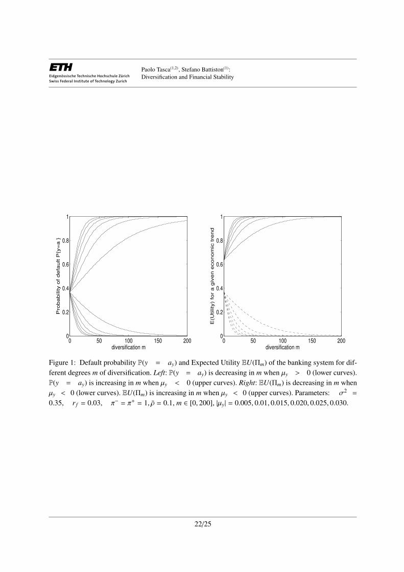
In words, Proposition 4 says that the benefit of diversification in external assets is influenced by thereturns generated by these activities. Essentially, In periods of upturn, banking diversification is desirablesince the probability of default will asymptotically be reduced to zero as m → ∞. While, in period ofdownturn, banking diversification is undesirable since the probability of default will asymptotically goesto one as m → ∞. (See Figure 1 in Appendix). The intuition behind this polarization of probability to“survive” and probability to “fail” is beguilingly simple, but its implications profound. In upturn periods,the system acts as a mutual insurance device with disturbances dispersed and dissipated. Connectivityengenders robustness. In this case, diversification would serves as a shock-absorber. But in downturn, thesystem flips the wrong side of the knife-edge. Diversification serve as shock-amplifiers, not dampener,as losses cascade.

4.3 Optimal Diversification Policy

By Proposition 3, the payoff from investment is external assets, is bounded.

Definition 4.1. Max Profit/Loss. The profit of the financial system is bounded between an upper bound aty = by and a lower bound at y = ay. Then, given the initial aggregate value of external assets yt=0 := y0,the gain from investment in external assets is π+ := by − y0; while, the loss is π− := y0 − ay.

10/25


Based on the management strategy in Definition 2.1, banks may choose from a finite setM of diversifi-cation strategies m, with m = 1, 2, .... It represents a set of mutually exclusive alternatives s.t. only one ofthem may be chosen in any period ∆t. The “buy and hold” asset allocation would be the following one.

Definition 4.2. Asset Allocation. Select the number m of external investments (assets and/or projects) inwhich to invest an equal dollar amount. Then, hold the selected assets for an arbitrary period ∆t.

The payoffs resulting from the choice of a diversification strategy m are represented by a random vari-able Πm that takes values π in the set Ωπ = [π−, ..., π+]. More specifically, given m alternatives 1, 2, ...and their corresponding random return Π1,Π2, ..., with distribution function F1(π), F2(π), ..., respectively,preferences satisfying the von Neumann-Morgenstern axioms imply the existence of a measurable, con-tinuous utility function U(π) such that Π1 is preferred to Π2 if and only if EU(Π1) > EU(Π2). Weassume banks are mean-variance decision makers, such that the utility function EU(Πm) may be writ-ten as a smooth function V

(E(Πm), σ2(Πm)

)13 of the mean E(Πm) and the variance σ2(Πm) of Πm or

V(E(Πm), σ2(Πm)

):= EU(Πm) = E(Πm) − (λσ2(Πm))/2 so that Π1 is preferred to Π2 if and only if

V(E(Π1), σ2(Π1)

)> V

(E(Π2), σ2(Π2)

). 14 Then, the maximization problem is

maxmEU(Πm) = E(Πm) −

λσ2(Πm)2

(10)

s.t.: m ≥ 1 ;1n

n∑i

m∑j

zi j = 1 .

To simplify notations, let p := P(µy ≤ 0); q := P(y = ay | µy < 0); g := P(y = ay | µy > 0). Then, theexpected profit E(Πm) of the financial system is

E(Πm) = p[qπ− + (1 − q)π+] + (1 − p)

[gπ− + (1 − g)π+] . (11)

In Table 1 in Appendix, the expected profit from banking diversification is considered in three differentstates of nature. (See Table 1 in Appendix). The variance σ2(Πm) of the profit is

σ2(Πm) = p[q(π− − E(Πm)

)2+ (1 − q)

(π+ − E(Πm)

)2]+ (1 − p)

[g(π− − E(Πm)

)2+ (1 − g)

(π+ − E(Πm)

)2].

(12)

Here below we conduct an analytical study of EU(Πm) for different values of parameters reported theTable 2 in Appendix.

13To say that V is smooth it is simply meant that V is a twice differentiable function of the parameters E(Πm) and σ2(Πm).14Only the first two moments matter for the decision maker, so the expected utility can be written as a function in

terms of the expected return (increasing) and the variance (decreasing) only, with ∂V(E(Πm), σ2(Πm)

)/∂E(Πm) > 0 and

∂V(E(Πm), σ2(Πm)

)/∂ σ2(Πm) < 0.

11/25


Analysis (i). In this analysis (10) is simplified since two mutually exclusive events are considered. First,the event downturn which occurs with probability p = 1. Second, the upturn event which occurs withprobability 1 − p = 1. In the downturn case, EU(Πm) is maximized for decreasing range of diversifica-tion. While, in the upturn case, EU(Πm) is maximized for increasing levels of diversification. Then, thefollowing holds true.

Corollary 1. Let mmax (mmin) be the max (min) attainable diversification strategy. Assume banks: (i)invest in external assets with dynamics defined in Proposition 1; (ii) use an allocation strategy as definedin 4.2; (iii) adopt a quadratic utility function of the form in (10). Then, in downturn, mmin mmax.Conversely, in upturn, mmax mmin.

Proof. See Appendix B.

The Corollary 1 follows immediately from Proposition 4. When external assets pay (with probabilityone) a negative or positive cash-flow, banks’ utility function in (10), respectively decreases or increaseswith increasing diversification. See results in Table 1, (Case 1 and Case 3) and see Figure 1 in Appendix.

Analysis (ii). In this analysis (10) is maximized w.r.t. m in the case the downturn and the upturn are twolikely events that might occur with some probability. Then, the following Proposition holds.

Corollary 2. Under the results in Corollary 1, let the event downturn (upturn) occur with probability p,(1 − p) where p ∈ ΩP := [0, 1]. Then, there exists a subset ΩP∗ ⊂ ΩP s.t., to each p∗ ∈ ΩP∗ , correspondsan optimal strategy m∗ ∈ (mmin,mmax) that maximizes the MV utility function in (10).


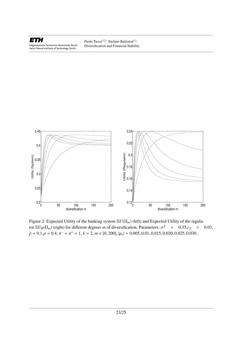
In words, let the absolute value of the trend to be given. Then, we assign a probability p to the eventdownturn and 1 − p to the upturn. Then, the expected utility EU(Πm) is computed for given q and g. Wefound that for certain values of p∗, there exist a specific optimal level of diversification m∗ which is afunction of p∗. (See Figure 2 in appendix). Corollary 2 suggests that only m∗ is the optimal diversificationstrategy that has to be chosen in order to maximize the expected MV utility. Values of m ≷ m∗ are second-best choices. In particular, for m approaching m∗ from below, the system increases its robustness, whilefor m bigger then m∗, the system is beyond its tipping point and becomes more fragile. Then the utilityfunction may exhibit a non-monotonic behavior with respect to m. (See Figure 2 in Appendix).

5 Private Incentives vs Social Welfare

Here we discuss the different implications of diversification at system level from a standpoint of a reg-ulator. Let’s consider the case of a policy maker that has to include some negative externalities which

12/25


might be engendered by losses occurred in downturn periods. Indeed, in an deeply downward trend, thewealth generated by the financial system is below the average-trend and might even be negative due togeneralized losses and failures. Because of deadweight costs of systemic failure that exceed the costs ofindividual failures, the regulator it is plausibly to consider social costs15 that might emerge due to thelosses suffered by the financial system. 16 Then, if K is the number of simultaneously crashing banks,treating the policy maker as an expected utility maximizer, it is reasonable to assume the followings.

Assumption 5.1 The total loss to be accounted by the regulator in downturn periods, is a monotonicallyincreasing function f (·) of (i) the expected number k of bank crashes given a collapse of at least one bankE(K|K ≥ 1) = k, (ii) the magnitude of the loss π−. Let the function f (·) be defined by f (k, π−) := kπ−.

Under this new perspective, the optimal diversification strategy (mR) from the policy maker point of viewdoes not coincide with the diversification desirable from the financial system point of view (m∗). Moreprecisely,

Corollary 3. Individual banks’ incentives favor a financial network that is over-diversified in externalassets w.r.t. to the level of diversification that is socially desirable

m∗ ≥ mR . (13)


In the presence of limited liability, the expected loss of an individual bank is bounded. In contrast, atthe system level, either due to direct or indirect exposures, the externalities associated with the failureof interconnected institutions under Assumption 4.1, amplify the expected losses. These reflect the in-cremental costs due to a system collapse which are ultimately borne by taxpayers. Under this condition,Corollary 3 says that the optimal level of diversification for the regulator is always smaller than the onedesirable at individual level.

6 Concluding Remarks

In this paper, we have combined the balance-sheet approach (Shin, 2008) with a stochastic setting a’ laMerton (1974). We consider a financial network of risk-averse banks, whose wealth is partially investedin assets external to the financial network, such as mortgages, loans to firms and other activities/projectsrelated to the real-side of the economy. Starting from the law of motion of the value of assets and liabil-ities, we developed a parsimonious, yet micro-founded, stochastic framework in which the fragility of abank depends on the fragility of the other banks and on the value of its external assets. In a mean-field

15Social costs include costs of financial distress and economic distress.16The definition of social losses is rather flexible since it depends on the characteristics of the financial system under analysis.

13/25


approximation, and under the assumption that banks choose the optimal number of external assets in aequally weighted portfolio, the failure probability can be derived analytically.

In this setting, we shed light on the conflict between one one hand the individual incentive to reduce,through diversification, the idiosyncratic risks of the external assets and, on the other hand, the emergenceof systemic risk. In contrast with some optimistic views about diversification, but in line with other recentworks (see e.g., Battiston et al., 2009; Ibragimov et al., 2011; Stiglitz, 2010; Wagner, 2009), we find thatdiversification fuels the double-edged property of the financial system. Indeed, diversification increasesthe default probability of the banking system in case external assets pay a negative cash-flow (downturn)and decreases the default probability in case of positive cash-flows (upturn).

Two main effects emerge in our model. The first is that the gap between maximal and minimal MVutility is exacerbated with higher degrees of diversification. Moreover, for a given fixed degree, the gapincreases the larger is the absolute value of the growth rate (i.e., higher the divergence of returns betweenthe up and down trend. This implies that, for a given probability of occurrence of the down(up) turn,there exists an optimal level of risk diversification which maximize the banking MV utility function.

By including in the analysis social costs due to generalized losses or defaults in case of a downturn,we obtain a final result. Individual banks’ incentives favor a financial network that is over-diversified inexternal assets w.r.t. to the level of diversification that is socially desirable. Thus, to preserve a stablefinancial system, diversification should be encouraged in periods of economic boom and constrained inperiods of recession. Nevertheless, as diversification of the financial system towards external activities isassumed to be a rigid strategy, the policy should be to adjust the system within a certain diversificationrange. In line with Ibragimov et al. (2011), our model suggests that policy restrictions to risk-sharing inupturn periods would limit excessive risk-spreading in downturn periods. Hence, an important point ofour analysis is in recognizing that the objective of the regulator is not to target a specific level of defaultrisk, but rather to manage the tradeoff between the social losses from defaults and the social costs ofavoiding defaults.

14/25


A Proofs

PROOF OF LEMMA 2.1. The leverage at banking system level can be described starting from (7) which can berewritten as

pi = φi

m∑j

Zi jy j +

n∑j

Wi j p j/(1 + r f + βφ j

)which at system dimension, becomes

p = Iφ ×[Zy + (R + βIφ)−1Wp

]= Φ ×

[Zy + (R + βΦ)−1Wp

]= ΦZy +Φ(R + βΦ)−1Wp.

Let define the column vector δ := Wp. Then,

p = ΦZy +Φ(R + βΦ)−1δ

pδT = ΦZyδT +Φ(R + βΦ)−1δδT

pδT(δδT)−1 = ΦZyδT(δδT)−1 +Φ(R + βΦ)−1

pδT(δδT)−1(R + βΦ) = ΦZyδT(δδT)−1(R + βΦ) +Φ.

Let ∆ := (δδT)−1 and let K := ZyδT∆. Then,

pδT∆R + pδT∆βΦ = ΦKR +ΦKβΦ +Φ

0 = ΦK[R + βΦ

]− pδT∆βΦ +Φ − pδT∆R

= ΦK[βΦ + R

]+Φ

[I − pδT∆β

]− pδT∆R,

which is a quadratic expression in Φ.

PROOF OF PROPOSITION 1. The portfolio composed by the linear combination of m processes described in(4), each of them weighted by 1/m, is

dy =1m

m∑j=1

µ jdt +1m

m∑i= j

σ jdB j = µydt + ... (14)

To derive the diffusion term, it is convenient to think about a sum of m Gaussian correlated error terms weightedby 1

m . Namely, 1m

∑mj=1 dB j which is equivalent to write 1

m∑m

j=1

√dtξ j with ξ j ∼ N(0, 1). Taking the variance yields

σ2y =

dt(m)2

m∑j=1

Var(ξ j)dt

(m)2

√Var(ξ j)Var(ξl)

m∑j=1

m∑j,l

ρ jl

=dtmσ2ξ +

dt(m)2

√σ2ξ jσ

2ξl

m∑j=1

m∑l,i

ρ jl,

(15)

15/25


where σ2ξ is the average variance among the m’s σ2

ξ j=1,...m. Since returns are assumed to be i.i.d., σ2

ξ jis constant, say

σ2 for all j = 1, ...,m. Then multiplying and dividing the second term of (15) by m − 1 and taking its square root,

we get σy :=√

σ2

m + m−1m ρσ2 where ρ =

∑mj=1

∑ml, j

ρ jl

m(m−1) and ξ ∼ N(0, 1). Hence (14) becomes

dy = µydt + σydB ∀i = 1, ..., n , (16)

where dB ∼ N(0, dt).

PROOF OF PROPOSITION 2. From Gardiner (1985), the probability that the leverage initially starting at anarbitrary level φ0 ∈ (aφ, bφ) exits through the default barrier bφ is

P(φ = bφ) :=∫ φ0

aφdφ′ψ(φ′)

/ ∫ bφ

aφdyψ(φ′)

, (17)

where ψ(φ′) = exp(∫ φ′

0 −2µφσ2φ

dφ). While µφ = yµy

∂ f (y)∂y + 1

2 y2σ2y∂2 f (y)∂y2 and σφ = yσy

∂ f (y)∂y are derived by Itos Lemma

applied to the function φ = f (y) given in (8) and using the dynamics of the process yt≥0 in (16).

PROOF OF PROPOSITION 3. First let observe that the partial derivative of φ w.r.t. y is negative. Thus, when ygoes up (down), φ goes down (up). This means that when φt≥0 touch the upper (lower) barrier, yt≥0 touches thelower (upper) corresponding barrier. Given the one-to-one function f : Ωy → Ωφ where φ = f (y) has the explicitform of (8); from f −1 : Ωφ → Ωy where y ∈ f −1(φ), we obtain the following mapping:

f (y) = 1 := bφ iff f −1(φ) = p(r f + β)/(R + β) := ay

f (y) = 0 := aφ iff f −1(φ) = p/2R := by .

Under this mapping, the default probability of the financial system is the probability P(y = ay) that yt≥0 exitthrough the default barrier p(r f + β)/(R + β) := ay instead of the safe barrier p/2R := by. Then, the defaultprobability can be expressed in two equivalent measures, as P(φ = bφ) or P(y = ay). Where P(y = ay) is theprobability that the process yt≥0 in (16), initially starting at an arbitrary level y0 ∈ (ay, by), exits through thedefault barrier ay := p(r f + β)/(R + β). From Gardiner (1985), this probability has the explicit form

P(y = ay) :=(∫ by

y0

dyψ(y))/

∫ by

ay

dyψ(y) ,

where ψ(x) = exp(∫ x

0 −2µy

σ2y

dy). Then, P(y = ay) has the closed form solution

P(y = ay) =

exp−2µyy0

σ2y

− exp−2µyb

σ2y

/ exp−2µya

σ2y

− exp−2µyb

σ2y

,where σy :=

√σ2

m + m−1m ρσ2, ay = p(r f + β)/(R + β), by = p/2R and y0 ∈ (ay, by).

PROOF OF PROPOSITION 4. Let us first provide an heuristic explanation of results in Proposition 3. Considerµy to be a random variable µy : Ωµy 7→ R defined on the probability space (Ωµy ,A,P) where Ωµy = [−1, 1] with

16/25


distribution function F : R→ R of µy as F(x) =∫ x−∞

f (t) dt = P(µy ≤ x) 17 To simplify notations, let p := P(µy ≤ 0);q := P(y = ay | µy < 0); g := P(y = ay | µy > 0). Now, let consider the solution of (16) i.e., y = y0 + µy + σyBtand for simplicity, let ρ = y0 = 0. The limit of y for m → ∞, yields a measurable function y = µy. Thus, y is alsoa random variable on Ωµy , since the composition of a measurable function is also measurable. Now let bound thevariation of y into an arbitrary small subset Ξ ⊂ Ωµy such that y ∈ [−ξ, ξ]. Then, for µy ≤ 1, the probability of y tobe equal to the upper bound is P(y = ξ | µy ≤ 1) = 1 − ε. While, for µy ≥ −1, the probability of y to be equal to thelower bound is P(y = −ξ | µy ≥ −1) = 1 − ε. We can now obtain a more formal asymptotic result if we substitute

−ξ and ξ with ay and by respectively. Let rewrite (9) as (My0 − Mby )/(May − Mby ) where M = exp(−2µy

σ2y

). After

some arrangements, P(y = a) becomes (My0−by )(May−by − 1) − 1/(May−by − 1). Taking the limit for m → ∞ we getthat µy > 0⇒ P(y = ay | µy > 0) = 0 − 0 = 0 and for µy < 0⇒ P(y = ay | µy < 0) = 0 − (−1) = 1. Then,

∀ε > 0, ∃ m > 1 | (q − g) > 1 − ε ∀m > m

PROOF OF COROLLARY 1. Based on the “state of nature” of external-assets, Corollary 1 shows the polariza-tion of the expected utility for increasing levels of diversification in those assets. The proof of Corollary 1 movesfrom the results in Proposition 4. Let first study P(y = ay) in (9) as a function of m and for the sake of simplicity,let ρ = β = r f = 0 and let σ = p = 1. 18. Then (9) becomes

P(y = ay) =(exp(−2µyy0m) − exp(−µym)

)/(1 − exp(−µym)

). (18)

When µy > 0 (µy < 0), (18) is negative (positive) for any parameters’ value in the set of Table 2. Its partialderivative w.r.t. m is

∂P(y = ay)∂m

= µy exp(µym(1 − 2y0)

) (exp(2µyy0m) − 1 + 2y0 − 2y0 exp(µym)

)/(exp(µym) − 1

)2,

which is equal to zero if µy = 0, negative if µy > 0 and positive if µy < 0. Stated otherwise, from the definitionof q and g, we have ∂q

∂m > 0 and ∂g∂m < 0. Let now, study how the utility function changes w.r.t. m in two mutually

exclusive cases. Namely, when the external assets are in upturn or downturn period for a certainty.

(1) The case p = 0 implies an upturn (i.e., µy > 0) and the utility function in (10) is simplified as

EU(Πm)µy>0 =(gπ− + (1 − g)π+) − λ (

g(π− − E(Πm)

)2+ (1 − g)

(π+ − E(Πm)

)2)/2 (19)

Then,∂EU(Πm)µy>0

∂m=

(π−

∂g∂m− π+ ∂g

∂m

)+∂g∂m

λ

2

(∆2

+ − ∆2−

),

where ∆2+ :=

(π+ −

∂g∂m (π− − π+)

)2and ∆2

− :=(π− − ∂g

∂m (π− − π+))2

. After some rearrangements

∂EU(Πm)µy>0

∂m= g

(∂g∂m

) (π− − π+) > 0 , (20)

17With the usual properties: (i) F(x) ≥ 0; (ii) limx→+∞

F(x) = limx→+∞

P(µy ≤ x) = P(µy < +∞) = 1; (iii) limx→−∞

F(x) = limx→−∞

P(µy ≤

x) = P(µy < −∞) = 0.18By Proposition 2, in this simplified case, y0 ∈ [0, 1/2]

17/25


which is positive since ∂g∂m < 0 and π− − π+ < 0. Then we conclude that, for p = 0, EU(Πm) is an increasing

function of m.

(2) In the case p = 1, there exists a downturn (i.e., µy < 0) and the utility function in (10) simplifies as

EU(Πm)µy<0 =(qπ− + (1 − q)π+) − λ (

q(π− − E(Πm)

)2+ (1 − q)

(π+ − E(Πm)

)2)/2 . (21)

Then,∂EU(Πm)µy<0

∂m=

(π−

∂q∂m− π+ ∂q

∂m

)+∂q∂m

λ

2

(Φ2

+ − Φ2−

),

where Φ2+ :=

(π+ −

∂q∂m (π− − π+)

)2and Φ2

− :=(π− − ∂q

∂m (π− − π+))2

. After some rearrangements,

∂EU(Πm)µy<0

∂m= q

(∂q∂m

) (π− − π+) < 0 , (22)

which is negative since ∂q∂m > 0 and π− − π+ < 0. Then we conclude that, for p = 1, EU(Πm) is a decreasing

function of m.

Summarizing, cases (1) and (2) lead to the following result µy < 0⇒ ∂EU(Πm)∂m < 0

µy > 0⇒ ∂EU(Πm)∂m > 0

∴ if

p = 0, V(E(Π), σ2(Π)

)mmax

> V(E(Π), σ2(Π)

)mmin⇐⇒ mmax mmin

p = 1, V(E(Π), σ2(Π)

)mmin

> V(E(Π), σ2(Π)

)mmax

⇐⇒ mmin mmax

where mmax (mmin) are respectively the max (min) attainable diversification strategies and stands for preferenceover strategies with x y is read “x i preferred to y”.

PROOF OF COROLLARY 2. The Corollary 2 shows that in the case the downturn and upturn events are bothlikely to occurs with certain probability, there might exists an optimal level of diversification m∗ which maximizesthe expected utility function EU(Πm) in (10). To prove it, let’s decompose (10) as follow

EU(Πm)µy>0 = (1 − p)[(

gπ− + (1 − g)π+) − λ2

(g(π− − E(Πm)

)2+ (1 − g)

(π+ − E(Πm)

)2)]

(23a)

EU(Πm)µy<0 = p[(

qπ− + (1 − q)π+) − λ2

(q(π− − E(Πm)

)2+ (1 − q)

(π+ − E(Πm)

)2)]. (23b)

Notice that (23a) and (23b) are respectively (19) and (21) used in Corollary 1 to which a probability p and 1− p tooccur, has been assigned. In other terms, (10) can be interpreted as a linear combination of (19) and (21). Now, letobserve that (23a) is increasing in m, while (23b) is decreasing in m

∂EU(Πm)µy>0

∂m= (1 − p)g

(∂g∂m

) (π− − π+) > 0 (24a)

∂EU(Πm)µy<0

∂m= pq

(∂q∂m

) (π− − π+) < 0 (24b)

18/25


When the partial derivatives in (24a) and (24b) are equal to each other, the EU(Πm) is maximized w.r.t. m. Thecondition to be verified is to find the probability p∗ that makes the two equations to be equivalent

FOC: (1 − p)g(∂g∂m

) (π− − π+) = pq

(∂q∂m

) (π− − π+) .

Discarding the trivial solution µy = 0, the condition is satisfied for all

p∗ = 1/(1 +

qg

(∂q∂g

))∈ ΩP∗ ⊂ ΩP := [0, 1] (25)

with q = q(m∗), g = g(m∗). Then, in a more general form, (25) can be written as p∗ = f [g(m∗); q(m∗)]. Since g, qand f are all one-to-one and hence invertible functions, for a fixed value of p∗, must exists an m∗ such that

m∗ =[(g−1; q−1) f −1

](p∗)⇒ ∃ EU(Πm∗ ) ≥ EU(Πm) ∀m ≷ m∗.

PROOF OF COROLLARY 3. From Assumption 5.1, the total loss accounted by the policy maker in downturnperiods is an increasing function of the expected number k of bank crashes given a collapse of at least one bankand the magnitude of the loss i.e., kπ−. Then, the expected utility of the regulator EUR(Πm) is differently expressedw.r.t. the utility from the bank point of view EU(Πm) i.e., EUR(Πm) , EUR(Πm). In particular, the changes involve(11) and (12) which are reformulated as follow

ER(Πm) = p[qkπ− + (1 − q)π+] + (1 − p)

[gπ− + (1 − g)π+]

σ2R(Πm) = p

[q(kπ− − E(Πm)

)2+ (1 − q)

(π+ − E(Πm)

)2]

+ (1 − p)[g(π− − E(Πm)

)2+ (1 − g)

(π+ − E(Πm)

)2].

Let follow the same reasoning used in Corollary 2 and decompose EUR(Πm) as follow

EUR(Πm)µy>0 = (1 − p)[(

gπ− + (1 − g)π+) − λ2

(g(π− − E(Πm)

)2+ (1 − g)

(π+ − E(Πm)

)2)]

(26a)

EUR(Πm)µy<0 = p[(

qkπ− + (1 − q)π+) − λ2

(q(kπ− − E(Πm)

)2+ (1 − q)

(π+ − E(Πm)

)2)]. (26b)

Let observe that the partial derivative w.r.t. m of (26b) is steeper then the partial derivative w.r.t. m in (24b). Inparticular,

∂EUR(Πm)µy<0

∂m= pq

(∂q∂m

) (kπ− − π+) < ∂EU(Πm)µy<0

∂m= pq

(∂q∂m

) (π− − π+) < 0

While∂EUR(Πm)µy>0

∂m≡∂EU(Πm)µy>0

∂m= (1 − p)g

(∂g∂m

) (π− − π+)

since (26a) is not affected by Proposition 5.1 and remains equivalent to (23a). The condition to be verified is tofind the probability pR that makes the two equations to be equivalent

FOC: (1 − p)g(∂g∂m

) (π− − π+) = pq

(∂q∂m

) (kπ− − π+) .

19/25


Discarding the trivial solution µy = 0, the condition is satisfied for all

pR = 1/(1 +

qg

(∂q∂g

)υ

)∈ ΩPR ⊂ ΩP := [0, 1] (27)

with q = q(mR), g = g(mR) and υ = (kπ− − π+)/(π− − π+). In a more general form, (27) can be written aspR = f (υ[g(m∗); q(m∗)]). Since g, q, υ and f are all one-to-one and hence invertible functions, for a fixed value ofpR, must exists an mR such that mR =

[(g−1; q−1) υ− f −1

](pR). Eq.(27) is a decreasing function w.r.t. υ which is

a constant function bigger than one as k > 1. Then, pR < p∗. This implies that the diversification level mR which isoptimal from the policy maker point of view is lower than the level m∗ desirable by the banking system

mR =[(g−1; q−1) υ−1 f −1

](pR) < m∗ =

[(g−1; q−1) f −1

](p∗)

20/25


B Tables

B.1 Expected Profit from Banking Diversification

Expected profit from banking diversification in the real-sectorExternal-assets trend p E(Πm) lim

m→+∞E(Πm)

Case 1 up 0 gπ− + (1 − g)π+ π+

Case 2 stable 0.5 (q+g)π−+(2−q−g)π+

2π++π−

2Case 3 down 1 qπ− + (1 − q)π+ π−

Table 1: Expected profit from banking diversification in case of up. stable and down trend of non-financial assets.

First, let remind (from Proposition 3), the asymptotic behavior of P(y = ay) for negative and positive values ofµy which gives lim

m→+∞q = 1 and lim

m→+∞g = 0. In Case 1, the expected profit of the banking system increases with

diversification because limm→+∞

g = 0. In Case 2, we implicitly assume that µy ∼ N(0, 1) since P(µy ≤ 0) = F(0) = 0.5.The expected profit asymptotically, for m → +∞, converges to (π+ + π−)/2. While for m → 1, both q and gconverge to one and the expected profit become E(π) = π− + π+. In Case 3, the expected profit decreases withbanking diversification because lim

m→+∞q = 1.

B.2 Range of values for Parameters

Parameter Set of Valuesm m ∈ N : m ≥ 1σ σ ∈ R : 0 < σ < 1r f r f ∈ R : 0 < r f < 1µy µy ∈ R : −1 ≤ µy ≤ 1ρ ρ ∈ R : 0 ≤ ρ ≤ 1by b ∈ R : by > 0ay a ∈ R : 0 < ay < b

Table 2: Range of values for each expl. variable.

C Figures

21/25


0 50 100 150 2000

0.2

0.4

0.6

0.8

1

diversification m

Pro

ba

bility o

f d

efa

ult P

y=

a

0 50 100 150 2000

0.2

0.4

0.6

0.8

1

diversification m

E(U

tility

) fo

r a

giv

en

eco

no

mic

tre

nd

Figure 1: Default probability P(y = ay) and Expected Utility EU(Πm) of the banking system for dif-ferent degrees m of diversification. Left: P(y = ay) is decreasing in m when µy > 0 (lower curves).P(y = ay) is increasing in m when µy < 0 (upper curves). Right: EU(Πm) is decreasing in m whenµy < 0 (lower curves). EU(Πm) is increasing in m when µy < 0 (upper curves). Parameters: σ2 =

0.35, r f = 0.03, π− = π+ = 1, ρ = 0.1, m ∈ [0, 200], |µy| = 0.005, 0.01, 0.015, 0.020, 0.025, 0.030.

22/25


0 50 100 150 2000.2

0.25

0.3

0.35

0.4

0.45

diversification m

Utility

(S

yste

m)

0 50 100 150 2000.12

0.14

0.16

0.18

0.2

0.22

0.24

diversification m

Utility

(R

eg

ula

tor)

Figure 2: Expected Utility of the banking system EU(Πm) (left) and Expected Utility of the regula-tor EUR(Πm) (right) for different degrees m of diversification. Parameters: σ2 = 0.35,r f = 0.03,ρ = 0.1,p = 0.4, π− = π+ = 1, k = 2, m ∈ [0, 200], |µy| = 0.005, 0.01, 0.015, 0.020, 0.025, 0.030 .

23/25


References

Acharya, V. (2009). A theory of systemic risk and design of prudential bank regulation. Journal ofFinancial Stability, 5(3):224–255.

Allen, F., Babus, A., and Carletti, E. (2010). Financial connections and systemic risk. Technical report,National Bureau of Economic Research.

Allen, F. and Gale, D. (2001). Financial contagion. Journal of Political Economy, 108(1):1–33.

Battiston, S., Gatti, D. D., Gallegati, M., Greenwald, B. C. N., and Stiglitz, J. E. (2009). Liaisonsdangereuses: Increasing connectivity, risk sharing and systemic risk. NBER Working Paper Seriesn.15611.

Brock, W., Hommes, C., and Wagener, F. (2009). More hedging instruments may destabilize markets.Journal of Economic Dynamics and Control, 33(11):1912–1928.

Eisenberg, L. and Noe, T. (2001). Systemic risk in financial systems. Management Science, 47(2):236–249.

Elsinger, H., Lehar, A., and Summer, M. (2006). Risk Assessment for Banking Systems. ManagementScience, 52(9):1301–1314.

Gai, P. and Kapadia, S. (2007). Contagion in financial networks. Bank of England, Working Paper.

Gardiner, C. W. (1985). Handbook of stochastic methods for physics, chemistry, and the natural sciences.Springer.

Haldane, A. (2009). Rethinking the financial network. Speech delivered at the Financial Student Asso-ciation, Amsterdam, April.

Haldane, A. and May, R. (2011). Systemic risk in banking ecosystems. Nature, 469(7330):351–355.

Ibragimov, R., Jaffee, D., and Walden, J. (2011). Diversification disasters. Journal of Financial Eco-nomics, 99(2):333–348.

Ibragimov, R. and Walden, J. (2007). The limits of diversification when losses may be large. Journal ofBanking and Finance, 31(8):2551–2569.

Iori, G., Jafarey, S., and Padilla, F. (2006). Systemic risk on the interbank market. Journal of EconomicBehaviour and Organization, 61(4):525–542.

May, R., Levin, S., and Sugihara, G. (2008). Complex systems: ecology for bankers. Nature,451(7181):893–895.

24/25


Merton, R. (1974). On the Pricing of Corporate Debt: The Risk Structure of Interest Rates. The Journalof Finance, 29(2):449–470.

Nier, E., Yang, J., Yorulmazer, T., and Alentorn, A. (2007). Network models and financial stability.Journal of Economic Dynamics and Control, 31(6):2033–2060.

Shin, H. (2008). Risk and Liquidity in a System Context. Journal of Financial Intermediation, 17:315–329.

Shin, H. (2009). Securitisation and financial stability. The Economic Journal, 119(536):309–332.

Stiglitz, J. E. (2010). Risk and global economic architecture: Why full financial integration may beundesirable. NBER Working Paper No. 15718.

Trichet, J.-C. (2009). Systemic Risk. Clare Distinguished Lecture in Economics and Public Policy.

Vega-Redondo, F. (2007). Complex Social Networks. Series: Econometric Society Monographs. Cam-bridge University Press.

Wagner, W. (2009). Diversification at financial institutions and systemic crises. Journal of FinancialIntermediation.

25/25

diversification and financial stability - chair of systems design

Documents