open canopy wind with parapets
TRANSCRIPT

8/22/2019 Open Canopy Wind With Parapets
http://slidepdf.com/reader/full/open-canopy-wind-with-parapets 1/275
ANALYSIS OF OPEN CANOPY
STRUCTURES WITH PARAPETS UNDER WIND
By
Augusto Poitevin Vera
A thesis submitted in partial fulfillment of the requirements for the degree of
DOCTOR OF PHILOSOPHY
In
CIVIL ENGINEERING
UNIVERSITY OF PUERTO RICOMAYAGUEZ CAMPUS
2009
Approved by:
Luis A. Godoy, Ph. D. Date
Chairman, Graduate Committee
Ricardo R. López, Ph. D. DateMember, Graduate Committee
Luis E. Suárez, Ph. D. Date
Member, Graduate Committee
Raúl E. Zapata López, Ph. D. Date
Member, Graduate Committee
Sonia Bartolomei, Ph. D. Date
Representative, Graduate Studies
Ismael Pagán Trinidad, MSCE. Date
Chairman, Civil Engineering & Surveying Department
8/22/2019 Open Canopy Wind With Parapets
http://slidepdf.com/reader/full/open-canopy-wind-with-parapets 2/275
ii
ABSTRACT
A literature review shows that there is a lack of information on the wind load pressures
acting on canopy structures with a parapet on the roof perimeter. On the other hand, a large
number of those structures suffered catastrophic damages due to hurricanes, for example during
Hurricanes Katrina and Rita in 2005. The latest version of the predominant standard and
commentary for wind design in the eastern part of the US, the ASCE 7-05, introduced for the
first time the issue of open structures. However, the code recommendations do not address open
structures with parapets. In this research, the author addresses the problem using two different
(but complementary) approaches: a numerical simulation using Computational Fluid Dynamics
(CFD) and wind tunnel testing. Values of pressure coefficients, Cp and Cn, were obtained with
the use of both methods, on top and bottom surfaces of the open canopy, and windward and
leeward surfaces for parapets, showing that the obtained values had good agreement between
both methodologies.
With the use of CFD, parametric studies further explore different plan geometries and
incremental parapet heights in order to obtain extreme Cn values. The obtained extreme values
were implemented on four case studies of collapsed open canopy structures, due to Hurricanes
Rita and Katrina in 2005. With the use of structural analysis software, the structural members
suffering extreme stresses, were identified and compared with the actual collapsed structures on
the case studies selected. Structural design procedure is suggested for the analysis of open
canopy structures with parapets and is implemented on each of the cases studied.
8/22/2019 Open Canopy Wind With Parapets
http://slidepdf.com/reader/full/open-canopy-wind-with-parapets 3/275
iii
RESUMEN
La revisión de la literatura demuestra la falta de información disponible sobre las
presiones de viento actuando sobre estructuras abiertas con parapetos en la periferia del techo de
las mismas. Por otra parte, un gran número de este tipo de estructuras sufren daños catastróficos,
por ejemplo durante los Huracanes Katrina y Rita que ocurrieron en el año 2005. La más reciente
versión del estándar y comentario en la parte Este de los Estados Unidos, el ASCE 7-05,
introdujo por vez primera el tema de las estructuras abiertas. Es de notar, que las
recomendaciones de este código no incluyen las estructuras abiertas con parapetos. En esta
investigación, el autor investiga el problema usando dos enfoques distintos, pero
complementarios: Usando Dinámica Computacional de Fluidos (CFD) y pruebas hechas en un
túnel de viento, valores de presión, Cp y Cn fueron obtenidos con el uso de ambos métodos, en
las superficies superiores e inferiores de la estructura abierta, y sotavento y barlovento en las
superficies de los parapetos, siendo los valores obtenidos muy parecidos entre ambas
metodologías.
Mediante el uso de CFD, estudios paramétricos exploran más profundamente diferentes
geometrías en planta y diferentes alturas para poder obtener valores Cn extremos. Estos valores
son entonces implementados en estudio de casos particulares, de estructuras abiertas que
colapsaron debido a los efectos de los Huracanes Katrina y Rita en el año 2005. Con el uso de un
programa de análisis de estructuras, miembros que sufrieron esfuerzos máximos, pudieron ser
identificados y comparados con las estructuras colapsadas en los casos seleccionados. Un
8/22/2019 Open Canopy Wind With Parapets
http://slidepdf.com/reader/full/open-canopy-wind-with-parapets 4/275
iv
procedimiento de diseño estructural para estructuras abiertas con parapetos es sugerido e
implementado para cada uno de los casos estudiados.

8/22/2019 Open Canopy Wind With Parapets
http://slidepdf.com/reader/full/open-canopy-wind-with-parapets 5/275
v
DEDICATION
I would like to dedicate this work, to my wife Yvonne and to my daughter Amanda. All
the time and effort during all this years, those two beautiful ladies were near me, encouraging me
and supporting me. I will be forever grateful for all the help, love and support from them during
all this time.

8/22/2019 Open Canopy Wind With Parapets
http://slidepdf.com/reader/full/open-canopy-wind-with-parapets 6/275
vi
ACKNOWLEDGEMENTS
I would like to thank Dr. Luis A. Godoy. Thank you for your patience and support during
all these years. Besides being my mentor, I consider him a very good friend. In addition, I would
like to thank Dr. Bruno Natalini, from the Universidad Nacional del Nordeste (UNNE) for the
help and support on the experimental part of this research. Thank you for all the help.

8/22/2019 Open Canopy Wind With Parapets
http://slidepdf.com/reader/full/open-canopy-wind-with-parapets 7/275
vii
TABLE OF CONTENTS
LIST OF FIGURES ....................................................................................................................... xi
LIST OF TABLES ..................................................................................................................... xxiii
LIST OF APPENDIX ................................................................................................................ xxiv
CHAPTER 1 PROBLEM STATEMENT ........................................................................................1
1.1 General information ...............................................................................................................1
1.2 Motivation ..............................................................................................................................3
1.3 Importance ..............................................................................................................................8
1.4 Objectives ...............................................................................................................................8
1.5 Proposed Methodology ..........................................................................................................9
1.6 Original Contributions ..........................................................................................................12
CHAPTER 2 LITERATURE REVIEW ........................................................................................13
2.1 Introduction ..........................................................................................................................13
2.2 Open Canopies .....................................................................................................................13
2.3 Computational Fluid Dynamics (CFD) ................................................................................19
2.4 Wind Tunnel Testing ............................................................................................................21
2.5 Parapet Pressures ..................................................................................................................22

8/22/2019 Open Canopy Wind With Parapets
http://slidepdf.com/reader/full/open-canopy-wind-with-parapets 8/275
viii
CHAPTER 3 SIMULATION OF WIND FLOW USING COMPUTATIONAL FLUID
DYNAMICS (CFD) .......................................................................................................................24
3.1 Theoretical Background .......................................................................................................24
3.2 EFD.Lab program description ..............................................................................................32
3.3 CFD model ...........................................................................................................................32
CHAPTER 4 WIND TUNNEL TESTING ....................................................................................46
4.1 General features of wind tunnel studies ...............................................................................46
4.2 Wind tunnel description .......................................................................................................48
4.3 Construction of models ........................................................................................................53
4.4 Instrumentation .....................................................................................................................58
4.5 Data processing ....................................................................................................................62
CHAPTER 5 AVAILABLE DESIGN CODE INFORMATION ..................................................66
5.1 General code information .....................................................................................................66
5.2 UBC 97 .................................................................................................................................66
5.3 ASCE 7-05 ...........................................................................................................................67
5.4 IBC 2006 ..............................................................................................................................69
5.5 Additional building codes ....................................................................................................69
CHAPTER 6 RESULT OF WIND PRESSURES IN CANOPIES ...............................................71
6.1 Comparison between wind tunnel results and previous work ..............................................71
6.2 CFD and wind tunnel results for top surface, wind at 0 degrees .........................................74

8/22/2019 Open Canopy Wind With Parapets
http://slidepdf.com/reader/full/open-canopy-wind-with-parapets 9/275
ix
6.3 CFD and wind tunnel results for bottom surface, wind at 0 degrees ...................................77
6.4 CFD and wind tunnel results for top surface, wind at 30 degrees .......................................78
6.5 CFD and wind tunnel results for bottom surface, wind at 30 degrees .................................79
6.6 CFD and wind tunnel results for parapets, wind at 0 degrees ..............................................83
6.7 CFD and wind tunnel results for parapets, wind at 30 degrees ............................................94
CHAPTER 7 PARAMETRIC STUDIES OF PRESSURE COEFFICIENTS IN CANOPIES
USING CFD.................................................................................................................................106
7.1 Description .........................................................................................................................106
7.2 Open canopy models, 7.6 m (25 ft) x 7.6 m (25 ft) at 0 degrees ........................................109
7.3 Open canopy models, 7.6 m (25 ft) x 7.6 m (25 ft) at 30 degrees ......................................116
7.4 Open canopy models, 7.6 m (25 ft) x 12.2 m (40 ft) at 0 degrees ......................................123
7.5 Open canopy models, 7.6 m (25 ft) x 12.2 m (40 ft) at 30 degrees ....................................129
7.6 Open canopy models, 7.6 m (25 ft) x 15.2 m (50 ft) at 0 degrees ......................................137
7.7 Open canopy models, 7.6 m (25 ft) x 15.2 m (50 ft) at 30 degrees ....................................144
7.8 Conclusions ........................................................................................................................150
CHAPTER 8 CASE STUDIES OF CANOPIES AND COMPARISONS WITH FIELD
EVIDENCE..................................................................................................................................152
8.1 Structural analysis ..............................................................................................................152
8.2 Case study #1, Shell Gas Station at Pt. Arthur, Texas, Method #1 ....................................154
8.3 Case study #1, Shell Gas Station at Pt. Arthur, Texas, Method #2 ....................................161

8/22/2019 Open Canopy Wind With Parapets
http://slidepdf.com/reader/full/open-canopy-wind-with-parapets 10/275
x
8.4 Case study #1, Shell Gas Station at Pt. Arthur, Texas, Method #3 ....................................164
8.5 Case study #2, Texaco Gas Station, Port Arthur, Texas ....................................................172
8.6 Case study #3, Chevron Gas Station, Vidor, Texas ...........................................................179
8.7 Case study #4, Exxon Gas Station, Hillerbrandt, Texas ....................................................186
8.8 Conclusions drawn from the Case Studies .........................................................................193
CHAPTER 9 CONCLUSIONS, ORIGINAL RESULTS, FUTURE RESEARCH AND
RECOMMENDATIONS .............................................................................................................194
9.1 Conclusions ........................................................................................................................194
9.2 Original results ...................................................................................................................196
9.3 Future research ...................................................................................................................198
9.4 Final recommendations ......................................................................................................199
REFERENCES ............................................................................................................................201
APPENDIX ..................................................................................................................................210

8/22/2019 Open Canopy Wind With Parapets
http://slidepdf.com/reader/full/open-canopy-wind-with-parapets 11/275
xi
LIST OF FIGURES
Figure 1.1. Schematic view of a canopy used in gas stations ..........................................................2
Figure 1.2. Open canopy of a Gas Station, Quebradillas, PR, (Photograph by the Author)............3
Figure 1.3. Failed canopy in Chalmette, New Orleans, during Hurricane Katrina ..........................5
Figure 1.4. Canopy structure collapsed at Meraux, New Orleans, Hurricane Katrina,
(Photograph by Godoy)....................................................................................................................5
Figure 1.5. Lateral deflections of open canopy due to wind pressures ............................................7
Figure 1.6. Stress ratio of open canopy members using ASCE 7-98 and AISC 89 .........................7
Figure 1.7. Flow and wind pressure distribution in the longitudinal direction ..............................10
Figure 1.8. Flow and wind pressure distribution in the transversal direction ................................10
Figure 1.9. Wind tunnel at UNNE, photograph by B. Natalini .....................................................11
Figure 2.1. Pressure gages used on Gumley’s investigation ..........................................................14
Figure 2.2. Model used on Altman study, at Clemson University, USA. (Photograph by the
Author) ...........................................................................................................................................15
Figure 2.3. Wind tunnel model (Uematsu et al. 2008)...................................................................17
Figure 2.4. Pressure taps arrangement (Uematsu et al. 2008) .......................................................18
Figure 3.1. Model of an infinitesimal small element assumed fixed in space ...............................26

8/22/2019 Open Canopy Wind With Parapets
http://slidepdf.com/reader/full/open-canopy-wind-with-parapets 12/275
xii
Figure 3.2. Computational domain for Model #1, with boundary definition and laminar wind
profile. The inlet condition is defined in the plane of the left ........................................................34
Figure 3.3. Computational domain for Model #2, without boundary definition and uniform
wind profile ....................................................................................................................................35
Figure 3.4. Computational domain for Model #3, without boundary definition and uniform
wind profile ....................................................................................................................................36
Figure 3.5. Model #1 top surface Cp values ..................................................................................37
Figure 3.6. Model #2 top surface Cp values ..................................................................................37
Figure 3.7. Model #3 top surface Cp values ..................................................................................38
Figure 3.8. Computational domain and meshing used on Model #3 .............................................40
Figure 3.9. Open canopy showing mesh, submeshing and further meshing at Model #3,
domain intercept .............................................................................................................................41
Figure 3.10. Pressure tap locations on top, bottom and parapet surfaces used for CFD
and wind tunnel scale model ..........................................................................................................42
Figure 3.11. Location of pressure taps and measured wind pressures on the top surface.
Wind direction acting from the right (0 degrees) ...........................................................................43
Figure 3.12. Model pressure taps on the canopy model ................................................................43
Figure 3.13. Wind direction in CFD model at 0 degrees ...............................................................44
Figure 3.14. Wind direction in CFD model at 30 degrees .............................................................45
Figure 4.1. View of the UNNE wind tunnel facility. (Photograph by the Author) .......................49

8/22/2019 Open Canopy Wind With Parapets
http://slidepdf.com/reader/full/open-canopy-wind-with-parapets 13/275
xiii
Figure 4.2. Typical Irwin spires used on the UNNE wind tunnel ..................................................51
Figure 4.3. View the UNNE surface roughness and Irwin spires. (Photograph by the Author) ....51
Figure 4.4. Wind tunnel plan at UNNE (reproduced from Wittwer and Moller 2000) .................52
Figure 4.5. Mean velocity profiles at the UNNE wind tunnel (Wittwer and Moller 2000) ...........52
Figure 4.6. Model with parapets with PVC tubes and columns. (Photograph by the Author) ......55
Figure 4.7. Top view of the model, showing the distribution of 16 pressure taps on the top
surface of the canopy and parapets. (Photograph by the Author) ..................................................55
Figure 4.8. Distribution of pressure taps on the model with bundle of tubes and columns.
(Photograph by the Author) ...........................................................................................................56
Figure 4.9. Distribution of pressure taps on the model ..................................................................57
Figure 4.10. View of the model with parapets on the turntable (Photograph by the Author) .......57
Figure 4.11. View the pressure electronic transducer Honeywell 163PC. (Photograph by the
Author) ...........................................................................................................................................58
Figure 4.12. View of the Scanivale 48 D9-1/2 w/PVC tubes (Photograph by the Author) ...........59
Figure 4.13. View of the UNNE Keithley 2000 digital multimeter (Photograph by the Author) .60
Figure 4.14. View of the Van Essen 2500 Betz differential micro manometer (Photograph
by the Author) ................................................................................................................................61
Figure 4.15. View of the Pitot-Prandtl tube (Photograph by the Author) ......................................61
Figure 4.16. View of the UNNE tunnel fan (Photograph by the Author) ......................................62
Figure 4.17. Calibration data on model without parapets ..............................................................63

8/22/2019 Open Canopy Wind With Parapets
http://slidepdf.com/reader/full/open-canopy-wind-with-parapets 14/275
xiv
Figure 4.18. Photograph showing the author taking data from the wind tunnel test .....................63
Figure 4.19. Processed data for the calibration of the transducer ..................................................64
Figure 4.20. Processed data for the pressure coefficient Cp ..........................................................65
Figure 6.1. No parapets, net pressures, wind direction of 0° from Ginger et al. (1994) ................72
Figure 6.2. No parapets, wind tunnel net pressures, wind direction of 0°, present research .........72
Figure 6.3. No parapets, net pressures, wind direction of 30° (Ginger et al. 1994) ......................73
Figure 6.4. No parapets, wind tunnel net pressures, wind direction of 30°, present research .......73
Figure 6.5. Canopy surface nomenclature .....................................................................................75
Figure 6.6. Cp results from top surface from CFD (a) and wind tunnel (b) model for incident
wind at 0 degrees from the structural axis .....................................................................................76
Figure 6.7. Cp results from bottom surface from CFD (a) and wind tunnel (b) model
for incident wind at 0 degrees from the structural axis ..................................................................77
Figure 6.8. Cp results from top surface from CFD (a) and wind tunnel (b) model for incident
wind at 30 degrees from the structural axis ...................................................................................78
Figure 6.9. Cp results from bottom surface from CFD (a) and wind tunnel (b) model
for incident wind at 30 degrees from the structural axis ................................................................80
Figure 6.10. Cn results from CFD (a) and wind tunnel (b) model for incident wind
at 0 degrees from the structural axis ..............................................................................................81
Figure 6.11. Cn results from CFD (a) and wind tunnel (b) model for incident wind
at 30 degrees from the structural axis ............................................................................................82
8/22/2019 Open Canopy Wind With Parapets
http://slidepdf.com/reader/full/open-canopy-wind-with-parapets 15/275
xv
Figure 6.12. Cp and Cn results for CFD model at 0 degrees for (25x25x4 ft) canopy ..................83
Figure 6.13. Cp results at parapet surface #1 at 0 degrees from CFD (a) and wind tunnel (b) .....84
Figure 6.14. Cp results at parapet surface #2 at 0 degrees from CFD (a) and wind tunnel (b) .....85
Figure 6.15. Cp results at parapet surface #3 and #7 at 0 degrees from CFD (a) and wind
tunnel (b) .....................................................................................................................................86
Figure 6.16. Cp results at parapet surface #4 and #8 at 0 degrees from . CFD (a) and
wind tunnel (b) ...........................................................................................................................87
Figure 6.17. Cp results at parapet surface #5 at 0 degrees from CFD (a) and wind tunnel (b) .....88
Figure 6.18. Cp results at parapet surface #6 at 0 degrees from CFD (a) and wind tunnel (b) .....89
Figure 6.19. Cn results at parapet surface #1 and #2 at 0 degrees from . CFD (a) and wind
tunnel (b) ......................................................................................................................................90
Figure 6.20. Cn results at parapet surface #3 and #4 at 0 degrees for CFD (a) and wind
tunnel (b) .....................................................................................................................................91
Figure 6.21. Cn results at parapet surface #5 and #6 at 0 degrees for CFD (a) and wind
tunnel (b) .....................................................................................................................................92
Figure 6.22. Cn results at parapet surface #7 and #8 at 0 degrees for CFD (a) and wind
tunnel (b) ....................................................................................................................................93
Figure 6.23. Cp results at parapet surface #1 at 30 degrees for CFD (a) and wind tunnel (b) ......94
Figure 6.24. Cp results at parapet surface #2 at 30 degrees for CFD (a) and wind tunnel (b) ......95
Figure 6.25. Cp results at parapet surface #3 at 30 degrees for CFD (a) and wind tunnel (b) ......96
8/22/2019 Open Canopy Wind With Parapets
http://slidepdf.com/reader/full/open-canopy-wind-with-parapets 16/275
xvi
Figure 6.26. Cp results at parapet surface #4 at 30 degrees for CFD (a) and wind tunnel (b) ......97
Figure 6.27. Cp results at parapet surface #5 at 30 degrees for CFD (a) and wind tunnel (b) ......98
Figure 6.28. Cp results at parapet surface #6 at 30 degrees for CFD (a) and wind tunnel (b) ......99
Figure 6.29. Cp results at parapet surface #7 at 30 degrees for CFD (a) and wind tunnel (b) ....100
Figure 6.30. Cp results at parapet surface #8 at 30 degrees for CFD (a) and wind tunnel (b) ....101
Figure 6.31. Cn results at parapet surface #1 and #2 at 30 degrees for CFD (a) and
wind tunnel (b) .........................................................................................................................102
Figure 6.32. Cn results at parapet surface #3 and #4 at 30 degrees for CFD (a) and
wind tunnel (b) .........................................................................................................................103
Figure 6.33. Cn results at parapet surface #5 and #6 at 30 degrees for CFD (a) and
wind tunnel (b) .........................................................................................................................104
Figure 6.34. Cn results at parapet surface #7 and #8 at 30 degrees for CFD (a) and
wind tunnel (b) .........................................................................................................................105
Figure 7.1. Nomenclature used for description of open canopy investigation ............................107
Figure 7.2. Model #1, contour plan for Cn values for wind at 0 degrees ....................................110
Figure 7.3. Model #1, 3D contour plot for Cn values for wind at 0 degrees ...............................110
Figure 7.4. Model #3, contour plan for Cn values for wind at 0 degrees ....................................111
Figure 7.5. Model #3, 3D contour plot for Cn values for wind at 0 degrees ...............................112
Figure 7.6. Model #5, contour plan for Cn values for wind at 0 degrees ....................................113
Figure 7.7. Model #5, 3D contour plot for Cn values for wind at 0 degrees ...............................113
8/22/2019 Open Canopy Wind With Parapets
http://slidepdf.com/reader/full/open-canopy-wind-with-parapets 17/275
xvii
Figure 7.8. Model #7, contour plan for Cn values for wind at 0 degrees ....................................114
Figure 7.9. Model #7, 3D contour plot for Cn values for wind at 0 degrees ...............................115
Figure 7.10. Influence of parapet height. 2D graph of Cn values for all 7.6 m (25 ft) x 7.6 m
(25 ft) at 0 degrees .......................................................................................................................116
Figure 7.11. Model #2, contour plan for Cn values for wind at 30 degrees ................................117
Figure 7.12. Model #2, 3D contour plot for Cn values for wind at 30 degrees ...........................117
Figure 7.13. Model #4, contour plan for Cn values for wind at 30 degrees ................................118
Figure 7.14. Model #4, 3D contour plot for Cn values for wind at 30 degrees ...........................119
Figure 7.15. Model #6, contour plan for Cn values for wind at 30 degrees ................................120
Figure 7.16. Model #6, 3D contour plot for Cn values for wind at 30 degrees ...........................120
Figure 7.17. Model #8, contour plan for Cn values for wind at 30 degrees ................................121
Figure 7.18. Model #8, 3D contour plot for Cn values for wind at 30 degrees ...........................122
Figure 7.19. 2D graph of Cn values for all 7.6 m (25 ft) x 7.6 m (25 ft) at 30 degrees ...............123
Figure 7.20. Model #9, contour plan for Cn values for wind at 0 degrees ..................................124
Figure 7.21. Model #9, 3D contour plot for Cn values for wind at 0 degrees .............................124
Figure 7.22. Model #11, contour plan for Cn values for wind at 0 degrees ................................125
Figure 7.23. Model #11, 3D contour plot for Cn values for wind at 0 degrees ...........................125
Figure 7.24. Model #13, contour plan for Cn values for wind at 0 degrees ................................126
Figure 7.25. Model #13, 3D contour plot for Cn values for wind at 0 degrees ...........................127
Figure 7.26. Model #15, contour plan for Cn values for wind at 0 degrees ................................128
8/22/2019 Open Canopy Wind With Parapets
http://slidepdf.com/reader/full/open-canopy-wind-with-parapets 18/275
xviii
Figure 7.27. Model #15, 3D contour plot for Cn values for wind at 0 degrees ...........................128
Figure 7.28. 2D graph of Cn values for all 7.6 m (25 ft) x 12.2 m (40 ft) at 0 degrees ...............129
Figure 7.29. Model #10, contour plan for Cn values for wind at 30 degrees ..............................130
Figure 7.30. Model #10, 3D contour plot for Cn values for wind at 30 degrees .........................131
Figure 7.31. Model #12, contour plan for Cn values for wind at 30 degrees ..............................132
Figure 7.32. Model #12, 3D contour plot for Cn values for wind at 30 degrees .........................132
Figure 7.33. Model #14, contour plan for Cn values for wind at 30 degrees ..............................133
Figure 7.34. Model #14, 3D contour plot for Cn values for wind at 30 degrees .........................134
Figure 7.35. Model #16, contour plan for Cn values for wind at 30 degrees ..............................135
Figure 7.36. Model #16, 3D contour plot for Cn values for wind at 30 degrees .........................135
Figure 7.37. Graph of Cn values for all 7.6 m (25 ft) x 12.2 m (40 ft) at 30 degrees ..................136
Figure 7.38. Model #17, contour plan for Cn values for wind at 0 degrees ................................137
Figure 7.39. Model #17, 3D contour plot for Cn values for wind at 0 degrees ...........................138
Figure 7.40. Model #19, contour plan for Cn values for wind at 0 degrees ................................139
Figure 7.41. Model #19, 3D contour plot for Cn values for wind at 0 degrees ...........................139
Figure 7.42. Model #21, contour plan for Cn values for wind at 0 degrees ................................140
Figure 7.43. Model #21, 3D contour plot for Cn values for wind at 0 degrees ...........................141
Figure 7.44. Model #23, contour plan for Cn values for wind at 0 degrees ................................142
Figure 7.45. Model #23, 3D contour plot for Cn values for wind at 0 degrees ...........................142
Figure 7.46. 2D graph of Cn values for all 7.6 m (25 ft) x 15.2 m (50 ft) at 0 degrees ...............143

8/22/2019 Open Canopy Wind With Parapets
http://slidepdf.com/reader/full/open-canopy-wind-with-parapets 19/275
xix
Figure 7.47. Model #18, contour plan for Cn values for wind at 30 degrees ..............................144
Figure 7.48. Model #18, 3D contour plot for Cn values for wind at 30 degrees .........................145
Figure 7.49. Model #20, contour plan for Cn values for wind at 30 degrees ..............................146
Figure 7.50. Model #20, 3D contour plot for Cn values for wind at 30 degrees .........................146
Figure 7.51. Model #22, contour plan for Cn values for wind at 30 degrees ..............................147
Figure 7.52. Model #22, 3D contour plot for Cn values for wind at 30 degrees .........................148
Figure 7.53. Model #24, contour plan for Cn values for wind at 30 degrees ..............................149
Figure 7.54. Model #24, 3D contour plot for Cn values for wind at 30 degrees .........................149
Figure 7.55. Graph of Cn values for all 7.6 m (25 ft) x 15.2 m (50 ft) @ 30 degrees .................150
Figure 8.1. Proposed Cn values to be applied for Method #3 to the structural analysis
model............................................................................................................................................154
Figure 8.2. Canopy floor plan and elevations for Case study #1 .................................................155
Figure 8.3. Contours for wind pressures for open canopy Case #1 at 0 degrees .........................156
Figure 8.4. Contours for wind pressures for open canopy Case #1 at 30 degrees .......................156
Figure 8.5. Computer model with wind pressures applied to roof surface at 0 degrees ..............157
Figure 8.6. Computer model with wind pressures applied to roof surface at 30 degrees ............157
Figure 8.7. Etabs model for Case #1 showing the refined roof mesh and deflected shape of
the wind loading at (a) 0 degrees (b) 30 degrees .........................................................................158
Figure 8.8. Structural steel results from Etabs for Case #1, showing members stress
ratios using Method #1 for (a) wind at 0 degrees (b) wind at 30 degrees....................................160

8/22/2019 Open Canopy Wind With Parapets
http://slidepdf.com/reader/full/open-canopy-wind-with-parapets 20/275
xx
Figure 8.9. Roof canopy wind pressures for case #1, Method #2, wind at 0 degrees,
(+ means downward pressure, - means uplift pressure) ...............................................................161
Figure 8.10. Roof canopy wind pressures for case #1, Method #2, wind at 30 degrees,
(+ means downward pressure, - means uplift pressure) ...............................................................162
Figure 8.11. Structural steel results from Etabs showing members stress ratios using
Method #2 for (a) wind at 0 degrees (b) wind at 30 degrees .......................................................163
Figure 8.12. Maple output of Wind pressure calculations using proposed Cn values with
ASCE 7-05 procedure, Case #1 ...................................................................................................165
Figure 8.13. Maple output of Wind pressure results on parapets using ASCE 7-05
Cn values ......................................................................................................................................166
Figure 8.14. Roof canopy pressure Cn and wind pressures for case #1, + means downward
pressure, - means uplift pressure ..................................................................................................166
Figure 8.15. Structural model for Case #1 on Etabs ....................................................................167
Figure 8.16. Structural model for Case #1 on Etabs showing deflected shape due to wind
pressures .......................................................................................................................................168
Figure 8.17. Structural model on Etabs showing overstress ratios on roof steel members .........169
Figure 8.18. Case #1 collapsed roof layout showing some of the roof beam damages.
Permanent deformation is clearly shown on some of the roof members .....................................170
Figure 8.19. Case #1 partial collapsed roof from below. Bottom of roof cladding has
been taken away due to high wind pressures ...............................................................................170

8/22/2019 Open Canopy Wind With Parapets
http://slidepdf.com/reader/full/open-canopy-wind-with-parapets 21/275
xxi
Figure 8.20. Case #1 roof cladding and beam structural layout. Photograph showing
permanent deformation on roof members ....................................................................................171
Figure 8.21. Case #1, transversal view of the deformed and collapsed roof ...............................171
Figure 8.22. Case #1, close up photograph of roof beams showing buckling and extreme
corrosion damage .........................................................................................................................171
Figure 8.23. Canopy floor plan and elevations for Case study #2 ...............................................173
Figure 8.24. Maple output of wind pressure calculations using proposed Cn values with
ASCE 7-05 procedure, Case #2 ...................................................................................................175
Figure 8.25. Roof canopy pressure Cn and wind pressures for case #2, + means downward
pressure, - means uplift pressure ..................................................................................................176
Figure 8.26. Structural model on Etabs showing overstress ratios on steel columns ..................177
Figure 8.27. Case #2, open canopy structure completely collapsed ............................................177
Figure 8.28. Case #2, photograph showing a buckled round steel column .................................178
Figure 8.29. Case #2, closer photograph of the round steel column base ....................................178
Figure 8.30. Case #2, photograph showing the open canopy structure on top of the
gas pumps.....................................................................................................................................179
Figure 8.31. Case #2, photograph showing the roof beam layout ...............................................179
Figure 8.32. Canopy floor plan and elevations for Case study #3 ...............................................180
Figure 8.33. Maple output of wind procedure calculations using proposed Cn values
with ASCE 7-05 procedure, Case #3 ...........................................................................................182
8/22/2019 Open Canopy Wind With Parapets
http://slidepdf.com/reader/full/open-canopy-wind-with-parapets 22/275
xxii
Figure 8.34. Maple output of Wind pressure results on parapets using ASCE 7-05 Cn values ..183
Figure 8.35. Roof canopy pressure Cn and wind pressures for case #3, + means downward
pressure, - means uplift pressure ..................................................................................................183
Figure 8.36. Structural model on Etabs showing overstress ratios of roof steel members
for Case #3 ...................................................................................................................................184
Figure 8.37. Case #3, open canopy photograph of the inverted steel structure after the steel
columns failed due to corrosion and wind pressures ...................................................................185
Figure 8.38. Case #3, photograph of the existing corrosion condition at the column base .........185
Figure 8.39. Case #3, additional photograph of the inverted steel structure ...............................186
Figure 8.40. Canopy floor plan and elevations for Case study #4 ...............................................187
Figure 8.41. Maple output of wind pressure calculations using proposed Cn values with
ASCE 7-05 procedure, Case #4 ...................................................................................................189
Figure 8.42. Roof canopy pressure Cn and wind pressures for Case #4, + means downward
pressure, - means uplift pressure ..................................................................................................190
Figure 8.43. Structural model on Etabs showing overstress ratios on all steel columns .............191
Figure 8.44. Case #4, photograph showing closer detail of the buckled steel columns ..............191
Figure 8.45. Case #4 photograph showing the collapsed steel columns ......................................192
Figure 8.46. Case #4, additional photograph of buckled steel columns. The photograph
shows the buckling of the internal column flange .......................................................................192
Figure 8.47. Case #4, upper roof beam layout on the collapsed open canopy roof .....................192

8/22/2019 Open Canopy Wind With Parapets
http://slidepdf.com/reader/full/open-canopy-wind-with-parapets 23/275
xxiii
LIST OF TABLES
Table 7.1. Model geometry description for the CFD parametric study .......................................108
Table 8.1. Table of wind pressures for case #1 to be used for the structural analysis .................167
Table 8.2. Table of wind pressures for case #2 to be used for the structural analysis .................176
Table 8.3. Table of wind pressures for case #3 to be used for the structural analysis .................184
Table 8.4. Table of wind pressures for case #4 to be used for the structural analysis .................190

8/22/2019 Open Canopy Wind With Parapets
http://slidepdf.com/reader/full/open-canopy-wind-with-parapets 24/275
xxiv
LIST OF APPENDIX
APPENDIX A. EFD.Lab modeling procedure ............................................................................210
APPENDIX B. Wind Tunnel Data ..............................................................................................217
APPENDIX C. Open canopy without parapets: spreadsheet calculations ..................................234
APPENDIX D. Open canopy with parapets: spreadsheet calculations .......................................238
APPENDIX E. Parapets: spreadsheet calculations ......................................................................242
APPENDIX F. CFD test of different wind angles .......................................................................246
APPENDIX G. T-test statistical analysis example ......................................................................250

8/22/2019 Open Canopy Wind With Parapets
http://slidepdf.com/reader/full/open-canopy-wind-with-parapets 25/275
1
CHAPTER 1. PROBLEM STATEMENT
1.1 General Information
Open canopies are frequently used in the construction of civil engineering facilities,
either as components of larger structures or as self supported structures. An example of the
second type may be found in most gas stations throughout the nation, in which the roof covers
the gas pumps and incoming vehicles. There are many other applications, including parts of
industrial buildings and processing plants, and sport courts. A large number of such structures
suffered catastrophic damages during hurricanes, including Hurricanes Katrina and Rita in 2005,
(NIST 2006).
In their typical configurations, open canopies are commonly supported by interior
columns in different patterns, without having any perimeter walls. The roof is formed by a
system of beams in two directions to support the roof panels. The supporting columns may be
aligned in one or more rows, depending on the size of the roof and on the functionality of the
facility. In small gas stations, canopies are frequently supported by a single row of columns as
illustrated in Figure 1.1. Typical dimensions vary from 6 m (20 ft.) to 15 m (50 ft.) in each
horizontal direction and from 3.7 m (12 ft.) to 6 m (20 ft.) in height.
From the structural point of view, it would be desirable to have a frame structure that
integrates columns and beams into a single resisting structure. However, the inspection of many
structures of this kind in the United States clearly shows that the beam-column connections are
not rigid connections, with the consequence that the majority of the connections used between
the elements are simple shear and tension connections. The majority of the canopy columns
inspected are designed as cantilever elements taking all the lateral forces due to wind pressure

8/22/2019 Open Canopy Wind With Parapets
http://slidepdf.com/reader/full/open-canopy-wind-with-parapets 26/275
2
and wind uplift. In addition, maintenance to open canopy structures appears to be a very
important factor that may reduce their factor of safety, but maintenance work is often neglected
with the consequence that corrosion is present in many canopies.
Figure 1.1: Schematic view of a canopy used in gas stations.
In hurricane-prone areas, such as the Caribbean islands and the coastal areas in the US,
the most critical structural conditions occur during high winds due to hurricanes. As it is known,
several hurricanes in recent years have been of category 3 and 4. This generates sustained wind
velocities of above 64.82 m/s (145 mph) in some regions, and those levels of wind velocities and
pressures have been incorporated in design codes such as ASCE 7-05, Figure 6-1. With such
high wind velocities, a surprise comes associated to the absence of information on the wind load
pressures acting on open structures with parapets. This void in our current state of knowledge is
also reflected in the design recommendations available to engineers and the catastrophic effects
on such structures due to the lack of design data and testing.
The majority of canopy structures have a parapet on the roof perimeter (as schematically
illustrated in Figure 1.1). The wind pressures that these types of structures are exposed to are

8/22/2019 Open Canopy Wind With Parapets
http://slidepdf.com/reader/full/open-canopy-wind-with-parapets 27/275
3
very complex, because pressures on the top and bottom surfaces of the roof are not uniform and
their values are different on each surface. Open canopy structures which include parapets have
not been studied in detail in the research literature or in the current codes used for design in the
United States.
1.2 Motivation
The predominant building code for wind design in the eastern part of the United States, is
the ASCE -7. It did not properly address the issue of open structures for a number of years. The
most recent version ASCE-7 05, was the first of various versions of this code that includes open
structures. However, it does not address the issue of open structures with parapets, which is
perhaps the most common configuration found in real constructions (see, for example Figure
1.2).
Figure 1.2: Open canopy of a Gas Station, Quebradillas, PR. (Photograph by the Author).
The pressure coefficients currently employed for the design of open canopy structures do
not include parapets on the structure perimeter. The Uniform Building Code, 1997 Edition, is the

8/22/2019 Open Canopy Wind With Parapets
http://slidepdf.com/reader/full/open-canopy-wind-with-parapets 28/275
4
predominant building code in the western part of the United States. This code addresses the issue
of open structures but does not provide any recommendations regarding the effects of parapets in
open structures.
In the event of a hurricane, the results on such structures have proven to be devastating.
Illustrations from some of 2005 hurricanes, Katrina and Rita, are shown in Figure 1.3 and Figure
1.4. The structure shown in Figure 1.3 was a new construction, completed during 2005. However
improper knowledge of the pressures acting due to wind effects may have been a major factor
contributing to the collapse. It was surprising during the field inspection in Texas and New
Orleans after hurricanes Katrina and Rita by Godoy (2006), the close relation of the poor
maintenance of open canopies and failure cases. There are several mechanisms leading to a rapid
deterioration of the structure: first, environmental action; second poor roof drainage (the drains
are located inside the hollow columns); and third, lack of preventive inspection.
Therefore, motivation to carry out this research is the need to establish basic
recommendations for the safe design of the main wind force resisting system (MWFRS) for such
structures. These recommendations will help in the proper maintenance and even possible retrofit
of existing structures and to improve their safety level.
8/22/2019 Open Canopy Wind With Parapets
http://slidepdf.com/reader/full/open-canopy-wind-with-parapets 29/275
5
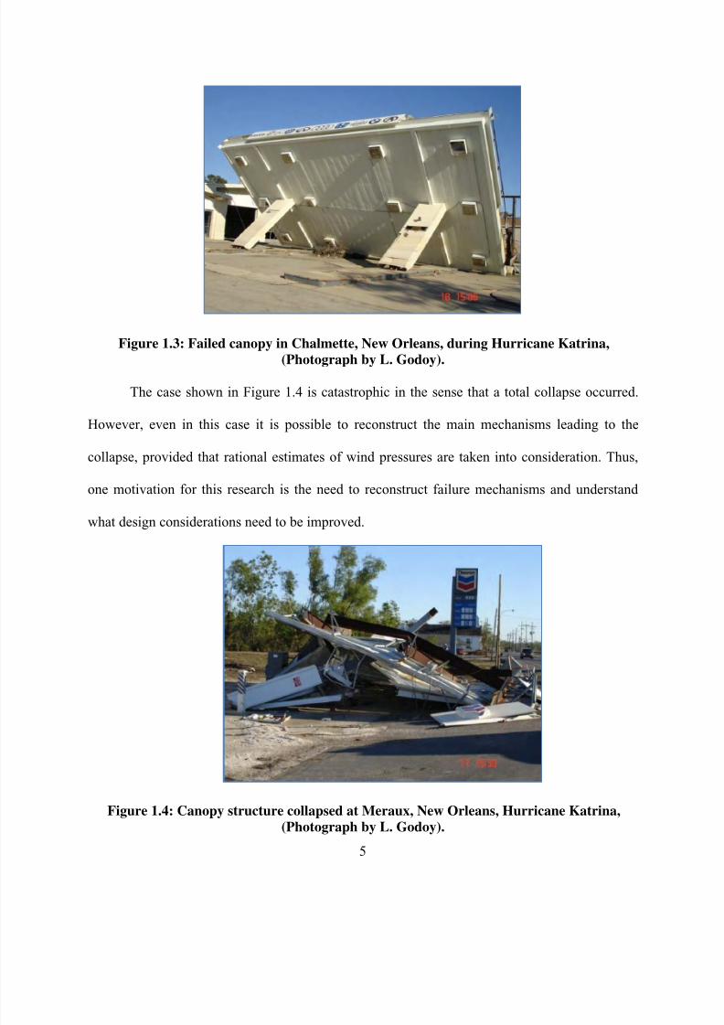
Figure 1.3: Failed canopy in Chalmette, New Orleans, during Hurricane Katrina,
(Photograph by L. Godoy).
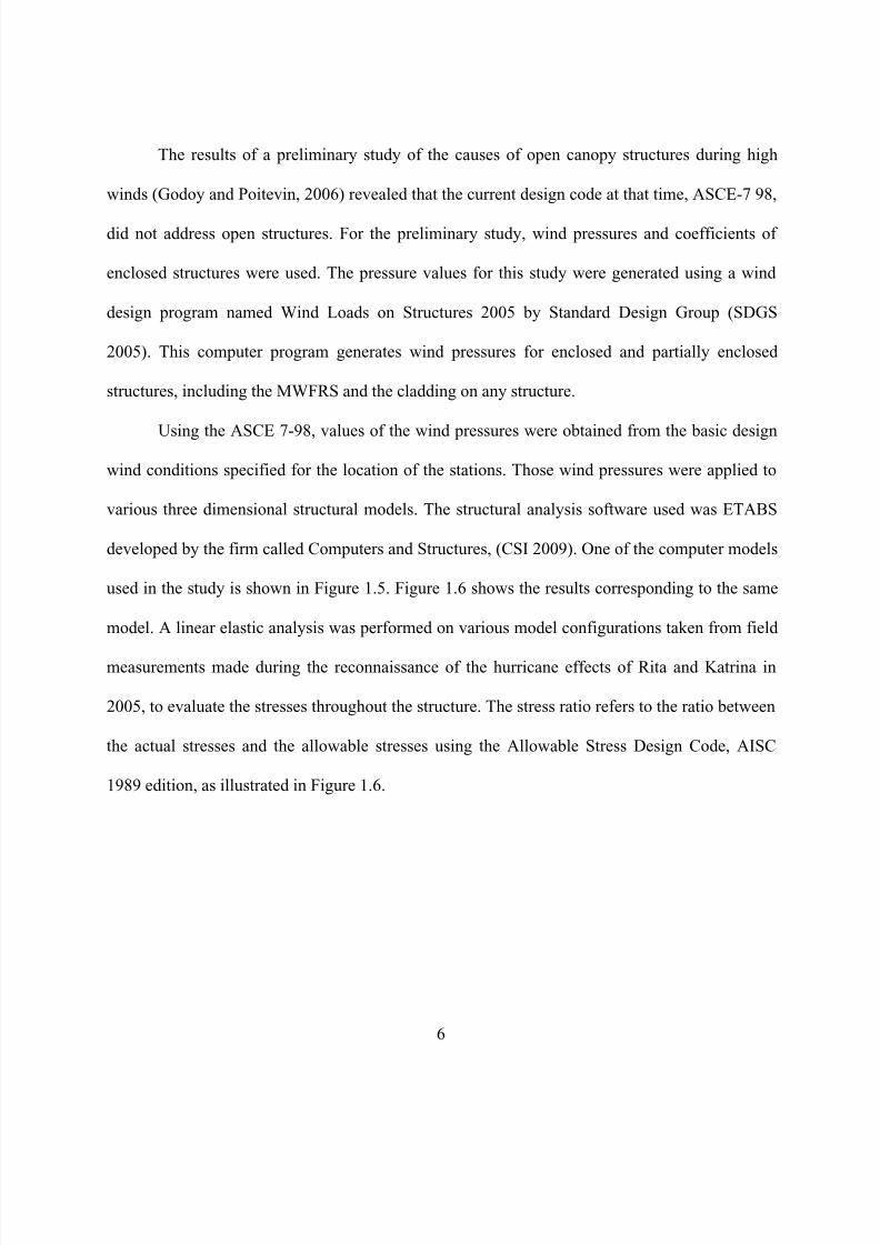
The case shown in Figure 1.4 is catastrophic in the sense that a total collapse occurred.
However, even in this case it is possible to reconstruct the main mechanisms leading to the
collapse, provided that rational estimates of wind pressures are taken into consideration. Thus,
one motivation for this research is the need to reconstruct failure mechanisms and understand
what design considerations need to be improved.
Figure 1.4: Canopy structure collapsed at Meraux, New Orleans, Hurricane Katrina,
(Photograph by L. Godoy).
8/22/2019 Open Canopy Wind With Parapets
http://slidepdf.com/reader/full/open-canopy-wind-with-parapets 30/275
6
The results of a preliminary study of the causes of open canopy structures during high
winds (Godoy and Poitevin, 2006) revealed that the current design code at that time, ASCE-7 98,
did not address open structures. For the preliminary study, wind pressures and coefficients of
enclosed structures were used. The pressure values for this study were generated using a wind
design program named Wind Loads on Structures 2005 by Standard Design Group (SDGS
2005). This computer program generates wind pressures for enclosed and partially enclosed
structures, including the MWFRS and the cladding on any structure.
Using the ASCE 7-98, values of the wind pressures were obtained from the basic design
wind conditions specified for the location of the stations. Those wind pressures were applied to
various three dimensional structural models. The structural analysis software used was ETABS
developed by the firm called Computers and Structures, (CSI 2009). One of the computer models
used in the study is shown in Figure 1.5. Figure 1.6 shows the results corresponding to the same
model. A linear elastic analysis was performed on various model configurations taken from field
measurements made during the reconnaissance of the hurricane effects of Rita and Katrina in
2005, to evaluate the stresses throughout the structure. The stress ratio refers to the ratio between
the actual stresses and the allowable stresses using the Allowable Stress Design Code, AISC
1989 edition, as illustrated in Figure 1.6.

8/22/2019 Open Canopy Wind With Parapets
http://slidepdf.com/reader/full/open-canopy-wind-with-parapets 31/275
7
Figure 1.5: Lateral deflections of open canopy due to wind pressures.
Figure 1.6: Stress ratio of open canopy members using ASCE 7-98 and AISC ASD89.
As said before, the latest version of the ASCE 7, the 2005 edition, addresses open
structures for the first time. Figure 6-18 of the ASCE 7-05 provide the design coefficients for
such structures. The studies for those coefficients provided by the code were performed on open
structures without parapets. This preliminary study opened a number of questions regarding the
wind pressures and structural response that motivated further studies to quantify both issues in
which the most complex part appeared to be the assessment of wind pressures.

8/22/2019 Open Canopy Wind With Parapets
http://slidepdf.com/reader/full/open-canopy-wind-with-parapets 32/275
8
1.3 Importance
Failures of open canopy structures are so common that during the event of a hurricane or
high winds, one does not need to specifically search for the collapse of those types of structures,
because they are easily found in most towns, as shown by the site reconnaissance made by
Godoy (2006). The collapse of an open canopy structure, in a gas station, interrupts the supply of
gasoline to the public and government agencies that need continued gas supply specially during
an emergency period. Therefore, this type of structures should be designed as a critical and of
high importance (essential facilities) in terms of human risks and security in the time of an
emergency. Unfortunately, this type of structure has been not been investigated in depth until the
current research, as shown by the literature review reported in Chapter 2. Research of open
structures without parapets has been conducted in several countries, including Australia, Canada,
Japan and in the United States. However, open canopy structures like those of gas stations have a
parapet on the perimeter of the roof. As mentioned before, the effects of that parapet and the
correlation between the height of the parapet and the geometry of the building are of crucial
importance to estimate wind pressures and have not been investigated in detail.
1.4 Objectives
The main objectives of this research may be divided in three major areas:
1. To investigate the characteristics of wind flow through open canopy structures with parapets,
in order to evaluate wind coefficients for the main wind force resisting system (MWFRS) due
to such conditions.

8/22/2019 Open Canopy Wind With Parapets
http://slidepdf.com/reader/full/open-canopy-wind-with-parapets 33/275
9
2. To explain the structural behavior of open canopy structures under wind, leading to the
identification of most severely stressed components and possibly of collapse mechanisms and
design problems.
3. To propose recommendations for design and future research based on rational basis for open
canopy structures with parapets.
1.5 Proposed Methodology
The proposed methodology in this work includes two stages. In a first stage, pressure
coefficients will be evaluated under the assumption of a rigid structure. In a second stage, the
pressure coefficients will be used as the loads acting on an elastically deformable structure to
estimate the response of the structure.
The first stage will be tackled by two different (but complementary) approaches: first, a
wind tunnel testing simulation will be carried out. Second, a computational simulation will be
performed using Computational Fluid Dynamics (CFD). A commercial CFD software named
EFD.Lab (Engineering Fluid Dynamics), developed by a firm called Flomerics (2009), will be
used for the computational fluid analysis. Such CFD simulation is able to calculate wind
pressures on the top and bottom surfaces of the structure with a wind velocity similar as those
specified by design codes such as ASCE 7 (2005). Factors such as turbulence, roughness,
humidity, and temperature can also be included in the CFD analysis to emulate real conditions.
As an introduction to the type of results expected from a CFD simulation, Figure 1.7 and 1.8
illustrate velocity field vectors as computed using EFD.Lab.

8/22/2019 Open Canopy Wind With Parapets
http://slidepdf.com/reader/full/open-canopy-wind-with-parapets 34/275
10
Figure 1.7: Flow and wind pressure distribution in the longitudinal direction.
Figure 1.8: Flow and wind pressure distribution in the transversal direction.
With the use of wind tunnel results, a calibrated CFD model can be used to explore various
models with different parapet heights. The wind tunnel facility used for this research is located at
the Universidad Nacional del Nordeste (UNNE) in Resistencia, Argentina. The UNNE wind
tunnel facility is a low velocity atmospheric boundary layer wind tunnel, built with the aim of
performing aerodynamic studies of structural models.
8/22/2019 Open Canopy Wind With Parapets
http://slidepdf.com/reader/full/open-canopy-wind-with-parapets 35/275
11
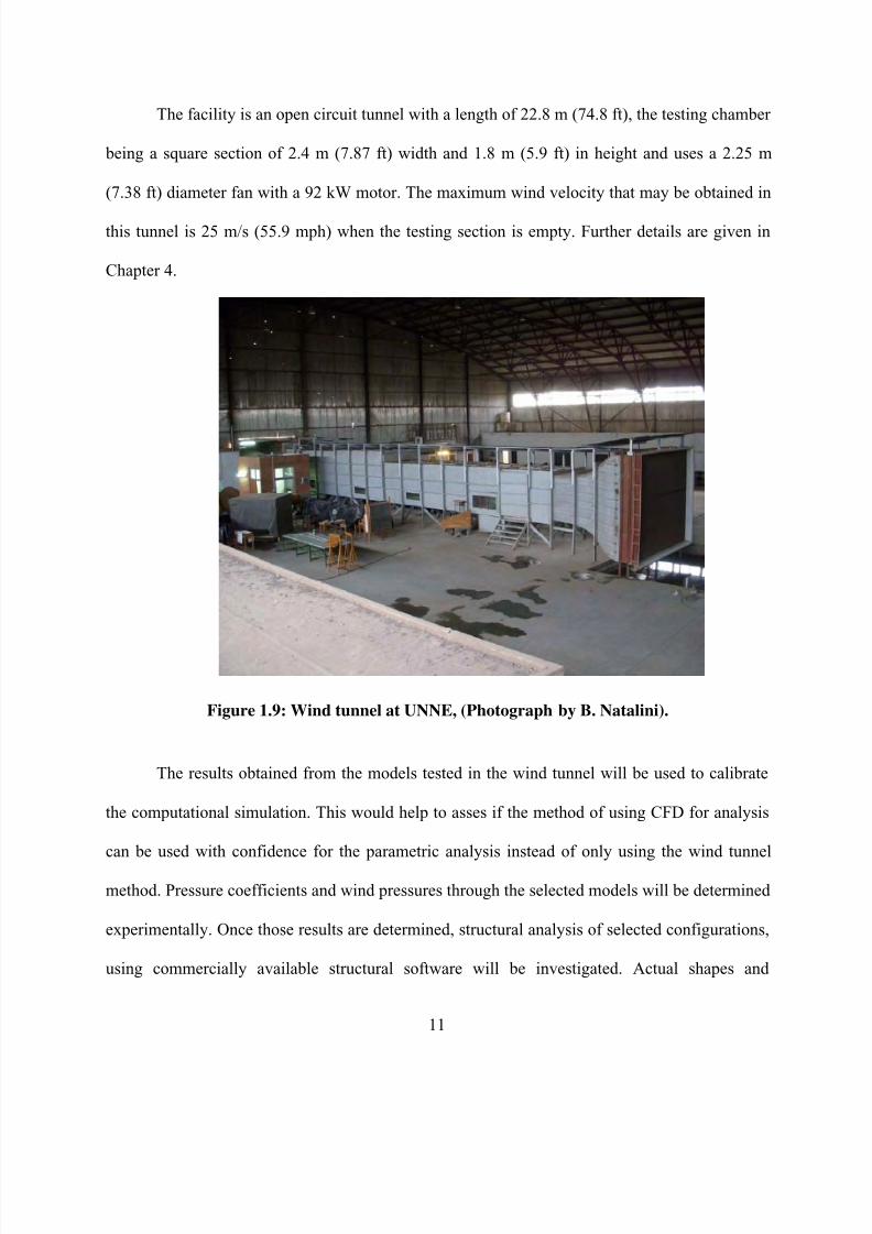
The facility is an open circuit tunnel with a length of 22.8 m (74.8 ft), the testing chamber
being a square section of 2.4 m (7.87 ft) width and 1.8 m (5.9 ft) in height and uses a 2.25 m
(7.38 ft) diameter fan with a 92 kW motor. The maximum wind velocity that may be obtained in
this tunnel is 25 m/s (55.9 mph) when the testing section is empty. Further details are given in
Chapter 4.
Figure 1.9: Wind tunnel at UNNE, (Photograph by B. Natalini).
The results obtained from the models tested in the wind tunnel will be used to calibrate
the computational simulation. This would help to asses if the method of using CFD for analysis
can be used with confidence for the parametric analysis instead of only using the wind tunnel
method. Pressure coefficients and wind pressures through the selected models will be determined
experimentally. Once those results are determined, structural analysis of selected configurations,
using commercially available structural software will be investigated. Actual shapes and
8/22/2019 Open Canopy Wind With Parapets
http://slidepdf.com/reader/full/open-canopy-wind-with-parapets 36/275
12
geometries of open canopy structures will be analyzed to assess their safety levels to withstand
design wind velocities.
1.6 Original Contributions
The proposed research will produce contributions to advance both, academic research and
engineering practice. On the academic front, pressure coefficients for the design of open canopy
structures with parapets do not exist at present. Open canopy structures without parapets have
been recently investigated and wind pressure distributions and design coefficients have been
proposed on a small number of previous investigations. However, no previous testing has been
reported with open canopy structures that consider the effects of parapets on wind flow. Because
this may be a controversial topic (due to its engineering significance), it is desirable to have
methodological redundancy to make sure that adequate pressure coefficients are reliable.
Correlation between the possible modeling and prediction of open canopy structures with the use
of CFD software has not been previously investigated. The possibility of the confirmation of the
use of CFD in the analysis of open canopy structures with parapets is another original
contribution of this research. Finally, a design procedure is needed to be used for the safe and
secure structural design of such structures.

8/22/2019 Open Canopy Wind With Parapets
http://slidepdf.com/reader/full/open-canopy-wind-with-parapets 37/275
13
CHAPTER 2. LITERATURE REVIEW
2.1 Introduction
The focus of this investigation is the effect of wind on open canopy structures with parapets.
This chapter contains a review of previous work presented by researchers on open canopies and
in the area of CFD, which is relevant to the current investigation. The literature review covers the
area of wind tunnel testing and parapet pressures.
2.2 Open Canopies
The past half century, has witnessed interesting developments in the understanding of wind
loading on structures. During this time, the description of wind load has moved from simple
static drag forces to sophisticated models (Davenport, 2002). A review of recent literature on
wind pressures in similar structures shows a wide variety of previous investigations. The need
for more detailed information on the wind flow and perhaps on open canopies is a consequence
of the collapse of a large number of open canopies in gas stations in areas affected by hurricanes
Katrina and Rita in 2005 (Godoy 2006).
Several researchers had the opportunity to study wind loads on open canopy structures.
Gumley (1984) made a parametric study investigating the effects of the roof shape, roof pitch,
roof aspect ratio, eave height, and wind direction and internal stacking arrangements. He
measured pressures averaged on roof areas using wind tunnel procedures. The effects of stacking
patterns under the roof were also investigated, but only the envelope results were presented.
Figure 2.1 shows the location of pressure gages used on Gumley’s investigation. The drawing is
interesting because it shows the number and location of pressure gauges employed by other

8/22/2019 Open Canopy Wind With Parapets
http://slidepdf.com/reader/full/open-canopy-wind-with-parapets 38/275
14
authors in wind tunnel tests. The results were used for updating the Eurocode (2002) and
Australian (1989) wind loading codes.
Figure 2.1: Pressure gages used on Gumley’s investigation
Full scale measures of agricultural canopy structures were reported by Robertson et al.
(1985). These structures had an aspect ratio l/b (length/width) of approximately 2. Based on
those results they proposed a set of wind force coefficients for designing such structures. Various
wind tunnel studies were subsequently carried to validate the conditions obtained from the full-
scale measurements by Robertson et al. (1985). Another set of experiments were performed by Letchford and Ginger (1992) and Ginger
and Letchford (1994), who measured the mean and peak point pressures over several roof areas.
They compared the obtained results with the Australian wind loading code at the time, to
conclude that the code provisions underestimated the wind loads. Altman (2001) made extensive
measurements of the forces and moments on mono-sloped and gable roofs at Clemson
University, USA. The roof models used in the study were made of high-density foam of 6 mm

8/22/2019 Open Canopy Wind With Parapets
http://slidepdf.com/reader/full/open-canopy-wind-with-parapets 39/275
15
thick. Figure 2.2 shows the model used on Altman’s study. He compared the obtained results
against various codes. In some cases, the code provisions underestimate and in others they
overestimated. From the measurements taken by Altman, based on the obtained experimental
results, he proposed wind force coefficients to be used for the design of main wind force
resisting systems.
Figure 2.2: Model used on Altman study, at Clemson University, USA. (Photograph by the
Author).
Letchford et al. (2000) measured mean wind forces on solid and porous canopy models.
The mean drag and lift forces on various open canopy roof geometries were investigated. In
conclusion, from the obtained result, the lift forces decrease as the pitch decreases and drag
forces increases as porosity increases. Lam and Zhao (2002) performed wind tunnel tests on
large cantilevered roofs, which are used mostly as grandstand roofs. The objective of the
investigation was to identify the generation mechanism of wind pressure and peak lifting action
on a large cantilevered roof. It was found that a horizontal roof is under a mean lifting action at

8/22/2019 Open Canopy Wind With Parapets
http://slidepdf.com/reader/full/open-canopy-wind-with-parapets 40/275
16
most wind incidence angles. However, at the wind incidence from the front of the roof, very high
suction was found on the front edge of the roof.
Natalini et al. (2002) investigated the pressure distribution on curved canopy roofs with
the use of wind tunnel testing. Curved canopy roofs are a very common type of structure in
South America. Mean pressure coefficient from the wind tunnel tests were presented on the
investigation. Paluch et al. (2003) investigated arch roof industrial buildings, adding the effect of
attached canopies on the sides. Six scale models with five different canopies were investigated.
The results showed that the aerodynamic coefficients for the roof are not affected by the
canopies, in the case of 0° from the main axis. However, the influence on the pressure
distribution is noticeable for wind incidence perpendicular to the main axis of the arch roofs and
for other incidences as well.
Uematsu et al. (2007) tested three types of roof geometries, (i.e. gable, troughed and
mono sloped roofs). Wind pressures were measured at many points both on the top and bottom
surfaces of the roof model at various wind directions. The conclusions at which Uematsu and co-
workers arrived based on their investigation and those of other authors may be summarized as:
a) The roof pitch affects the wind forces significantly.
b) There are significant differences in the results when the roof pitch is smaller than 15.
c) The influence of roof aspect ratio (length/width from 1 to 4) on the wind force
coefficients is small.
d)
The experimental data for mono sloped and gable roofs is limited.
e) Roof thickness and supporting systems significantly affects the results.
Roof is supported by slender columns and no walls, so that wind action is directly exerted
on the top and bottom surfaces. These roofs seem to be more vulnerable to wind actions than

8/22/2019 Open Canopy Wind With Parapets
http://slidepdf.com/reader/full/open-canopy-wind-with-parapets 41/275
17
those of enclosed buildings. Local wind pressures and overall wind forces and moments acting
on free standing canopy roofs have been investigated experimentally. Based on the results for the
distribution of the most critical positive and negative peak pressure difference coefficients
irrespective of wind direction, the peak wind force coefficients for the design of cladding and its
immediately supporting structures were proposed in Uematsu et al. (2007).
Figure 2.3: Wind tunnel model (Uematsu et al. 2008)
Figure 2.3 shows a canopy roof model on the turntable of the wind tunnel of Concordia
University. Special care was taken in decreasing the roof thickness and column width to avoid
the distortion of the flow around the roof. The roof model is made of two galvanized steel sheets
0.3 mm thick and consists of a sandwich structure.
8/22/2019 Open Canopy Wind With Parapets
http://slidepdf.com/reader/full/open-canopy-wind-with-parapets 42/275
18
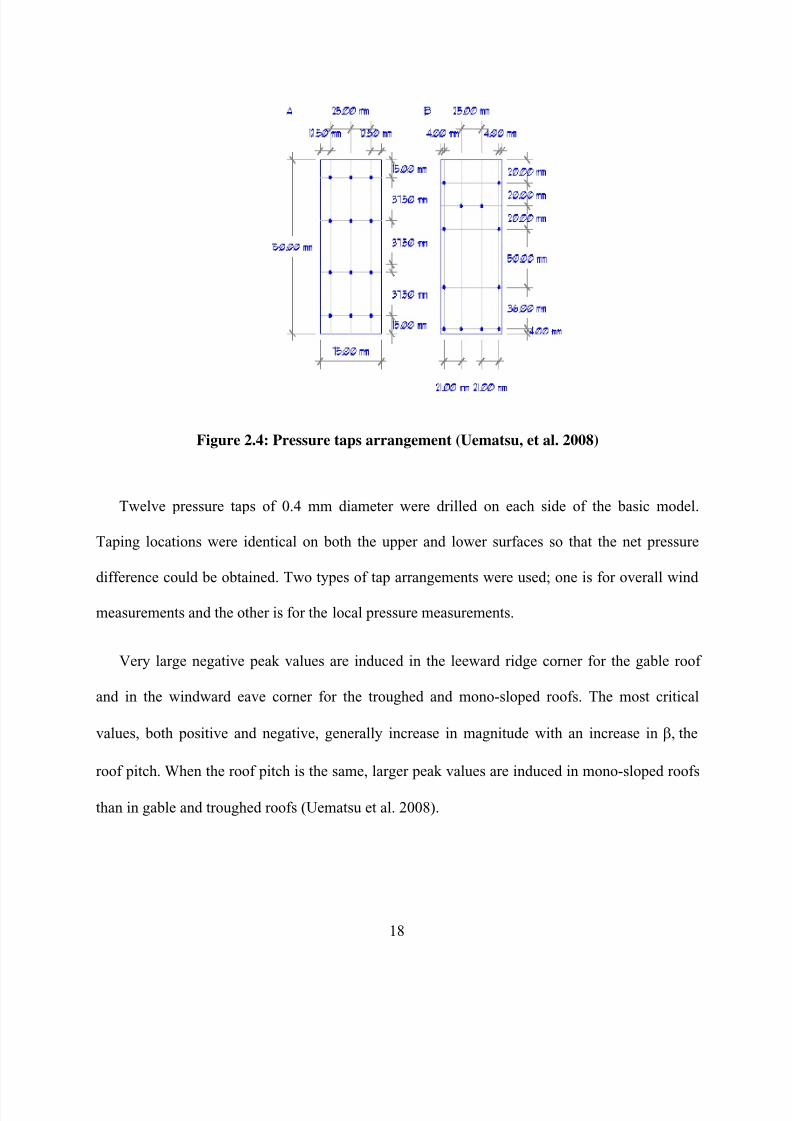
Figure 2.4: Pressure taps arrangement (Uematsu, et al. 2008)
Twelve pressure taps of 0.4 mm diameter were drilled on each side of the basic model.
Taping locations were identical on both the upper and lower surfaces so that the net pressure
difference could be obtained. Two types of tap arrangements were used; one is for overall wind
measurements and the other is for the local pressure measurements.
Very large negative peak values are induced in the leeward ridge corner for the gable roof
and in the windward eave corner for the troughed and mono-sloped roofs. The most critical
values, both positive and negative, generally increase in magnitude with an increase in the
roof pitchWhen the roof pitch is the same, larger peak values are induced in mono-sloped roofs
than in gable and troughed roofs (Uematsu et al. 2008).

8/22/2019 Open Canopy Wind With Parapets
http://slidepdf.com/reader/full/open-canopy-wind-with-parapets 43/275
19
2.3 Computational Fluid Dynamics (CFD)
Computational fluid dynamics (CFD) in Wind Engineering was initiated and has progressed
over the past two decades. The rapid growth of computer power, which makes possible power
acquisition and analysis of large amounts of experimental data, has led to the increasing use of
CFD techniques (Baker 2007). The ultimate goal of CFD is to represent the physical events that
occur in the fluids flow around and within designated objects. These events are related to the
action and interaction of dissipation, diffusion, convection, shock waves, slip surfaces, boundary
layers and turbulence. In the field of aerodynamics all these phenomena are governed by the
Navier-Stokes equations (Lomax and Pulliam, 1999).
Computational fluid dynamics constitutes a new approach in the study and development of
fluid dynamics, which was previously dominated by wind tunnel testing. At present, most
researchers in the field of wind engineering agree that there is a need to have better theory and
experiments in order to gain understanding of wind acting on structures. The recent success
obtained through CFD simulations are indicative that both, physical and numerical approaches
can be used as complementary techniques, rather than on eliminating the other. Computational
fluid dynamics results are analogous to wind tunnel results obtained in a laboratory, in the sense
that they both provide data for given flow configurations. However, unlike a wind tunnel which
is generally heavier, a computer program can be carried on and accessed remotely by computers
(Anderson, 1995).
Computational fluid dynamics (CFD) has recently made enormous strides. However,
techniques for obtaining time dependent pressures induced by turbulent flows do not allow the
routine and confident use of CFD as a substitute for wind tunnel testing of structures, although
8/22/2019 Open Canopy Wind With Parapets
http://slidepdf.com/reader/full/open-canopy-wind-with-parapets 44/275
20
can be a compliment for such testing. The role of CFD in structural engineering applications may
be expected to become more important in the future (Simiu and Miyata 2006).
Use is often made of commercially available CFD codes because of their ready availability,
well developed interfaces and broad verification and validation. The atmospheric boundary layer
(ABL) extends for a considerable distance above the earth’s surface relative to the average
building height. CFD can only represent a smaller finite distance because of hardware limitation
and the complexity of including a meteorological model. Currently, smaller features such as
vegetation and small buildings cannot be included in the computational grid using personal
computers. The k- model, that includes energy dissipation, is generally incorporated through a
wall function approach that is based on boundary layer theory (Hargreaves and Wright 2007).
Accurate simulation of ABL flow in the computer domain is imperative to obtain accurate
and reliable predictions of the related atmospheric process. In a CFD simulation, the flow
profiles of mean wind speed and turbulence quantities that are applied at the inlet plane of the
computational domain are generally fully developed profiles. These profiles should be
representative of the roughness characteristics of that part of the upstream terrain that is not
included in the computational domain. This is expressed by the presence of either the appropriate
aerodynamic roughness length or the appropriate power law exponent of the terrain (Blocken et
al. 2007).
The most common CFD techniques are capable of predicting the mean pressures on buildings
with reasonable accuracy, but are not sufficiently accurate at evaluating the fluctuating and peak
pressures. The poor representation of the pressure fluctuations is primarily because it is
necessary to incorporate over simplified representations of the turbulence in the fluid flow

8/22/2019 Open Canopy Wind With Parapets
http://slidepdf.com/reader/full/open-canopy-wind-with-parapets 45/275
21
equations. However, CFD techniques are capable of providing useful insights into wind flow
around building for environmental considerations (Holmes, 2001).
The lack of validation with the full scale, as was done in the early years on wind tunneling,
could easily mislead a well intentioned structural engineer into thinking that the CFD package is
generating real design loads. Engineers need to take the lead to ensure that non-validated data are
non taken as gospel (Cochran, 2006).
2.4 Wind Tunnel Testing
Wind tunnel testing was mostly carried out in aeronautical wind tunnels in smooth uniform
flow. There were some isolated exceptions where the variation of wind speed with height was
simulated. Although there were significant differences in the pressures between uniform and
boundary layer flows, it appeared to be of academic interest only (Davenport, 2002).
A significant development during the 1950s was due to Jensen, who undertook a comparison
of the mean pressures on small buildings in full scale and in wind tunnel model experiments.
They were carried out in a variety of boundary layers, and he stated his model law, “The correct
model test for phenomena in the wind must be carried out in a turbulent boundary layer and the
model law requires the boundary layer to be scaled as regards the velocity profile” (Davenport,
2002).
Wind tunnel test on wind loading on structures require the simulation of the atmospheric
boundary layer (ABL). Several methods have been proposed since 1960’s to reproduce the
atmospheric flow. It is accepted that the best atmospheric boundary layer simulation is obtained
with rough floor surface, although simulation scales reached by this method are too small for

8/22/2019 Open Canopy Wind With Parapets
http://slidepdf.com/reader/full/open-canopy-wind-with-parapets 46/275
22
usual applications in structural aerodynamics. It has been shown that when comparing with
atmospheric data, it is preferable to use comparative procedures, which do use the boundary
layer thickness as a scaling factor (De Bortoli et al. 2002).
Wind tunnels have evolved as an indispensable aid to the practice of civil engineering.
Boundary layer wind tunnels and currently data acquisition systems reveals that such tests
continue to provide even more comprehensive wind load information for structural design
(Cermark 2003).
With the basics of the aerodynamics of bluff bodies and the detailed characteristics of the
atmospheric surface layer discussed in the previous sections, one can now approach the wind
tunnel simulation process with confidence. The important element in the section on bluff body
aerodynamics is the role played by the turbulence (small scale and large scale) in the formation
of vortices under separated shear layers (Tieleman, 2003).
Independent tests conducted at six prominent wind tunnel laboratories on models of two
industrial buildings showed that test results can vary significantly from laboratory to laboratory.
Because of some variations in results, some structural engineering firms have engaged in the
design of important structures, commission wind tunnel tests to more than one laboratory (Simiu
and Miyata 2006).
2.5 Parapet Pressures
The influence of parapets has been investigated for closed structures, perhaps in relation to
wind effects on closed buildings. It is clear that low parapets may significantly increased the roof
corner suctions for oblique wind directions. Data indicates that, in general, the higher the

8/22/2019 Open Canopy Wind With Parapets
http://slidepdf.com/reader/full/open-canopy-wind-with-parapets 47/275
23
parapet, the lower are the pressure coefficients. This is due to the fact that the parapet tends to lift
the vortices away from the roof surface. A wind study reflecting a comparison with existing wind
code provisions, NBCC (National Building Code of Canada) and ANSI 1985, against obtained
experimental results on wind pressures and suctions on flat roofs with parapets (Stathopoulos
and Baskaran, 1987).
Pressure studies have shown that parapet height can influence pressure coefficients at the
roof edge. Low parapets, of the order of 0.5m in height, have been found to increase peak suction
on the roof in comparison to a roof without a parapet. On the other hand, higher parapets, in the
order of 1 m or higher, cause a significant reduction in peak suction (Stathopoulos et al. 2002).
The parapets tend to raise the corner vortex above the roof surface. For lower parapets, this
acts to increase the local suctions; for higher parapets, the loads are decreased below those of no
parapets. In all cases, the extents of the vortices on the roofs are expanded. The results of a
systematic study on the effects of parapets on structural loads for low buildings indicate that
parapets are no benign. The distance from the flow separation at the eave’s edge to the first
reattachment point on the roof for normal wind increases significantly. This leads to an increased
load of about 10% in interior frames. Bay uplift is increased on end bays by similar amounts
(Kopp et al. 2005).

8/22/2019 Open Canopy Wind With Parapets
http://slidepdf.com/reader/full/open-canopy-wind-with-parapets 48/275
24
CHAPTER 3. SIMULATION OF WIND FLOW USING
COMPUTIONAL FLUID DYNAMICS (CFD)
There are several ways to represent wind flow on structural components, either through a
physical representation of the structure (as would be done in a wind tunnel) or else using
computer modeling. This chapter deals with the computational simulation of wind flow on
structures using what is known as Computational Fluid Dynamics (CFD), whereas wind tunnel
representations are discussed in the next chapter.
3.1 Theoretical background
Computational fluid dynamics (CFD) techniques have been under development for a number
of years (Holmes 2001) as a branch of fluid dynamics. At present, CFD constitutes a new
approach in the study of wind effects on structures. The introduction of fast digital computers,
together with the development of accurate numerical algorithms for solving numerical problems,
has revolutionized the way researchers study and practice fluid dynamics today. This
complements the approaches of the pure theory and pure experiments but, as Anderson (1995)
states, it will never fully replace either of these approaches.
CFD results are directly analogous to wind tunnel results obtained in a laboratory; they both
represent sets of data for given flow configurations at different Mach numbers, Reynolds
numbers, etc. A CFD computer program is, therefore, a readily transportable tool, and could be
thought as analogous to a transportable wind tunnel (Anderson 1995).
The physical aspects of fluid flows are governed by three fundamental postulates:
1. Mass is conserved
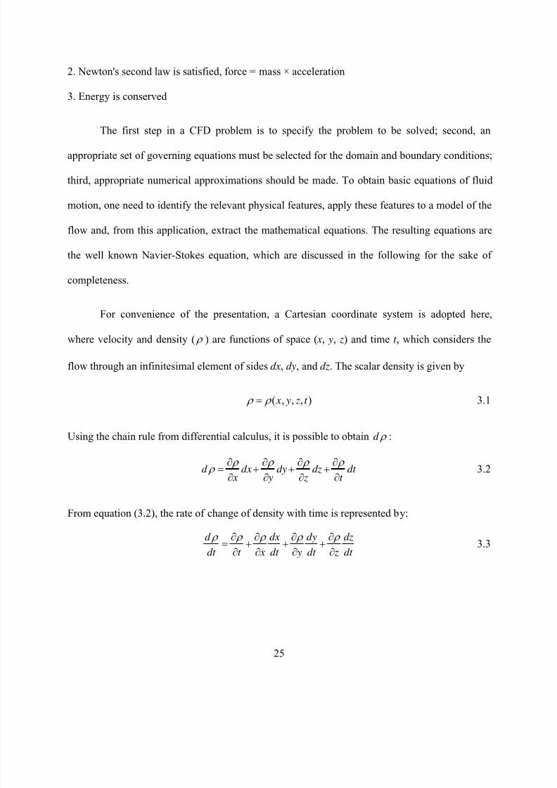
8/22/2019 Open Canopy Wind With Parapets
http://slidepdf.com/reader/full/open-canopy-wind-with-parapets 49/275
25
2. Newton's second law is satisfied, force = mass × acceleration
3. Energy is conserved
The first step in a CFD problem is to specify the problem to be solved; second, an
appropriate set of governing equations must be selected for the domain and boundary conditions;
third, appropriate numerical approximations should be made. To obtain basic equations of fluid
motion, one need to identify the relevant physical features, apply these features to a model of the
flow and, from this application, extract the mathematical equations. The resulting equations are
the well known Navier-Stokes equation, which are discussed in the following for the sake of
completeness.
For convenience of the presentation, a Cartesian coordinate system is adopted here,
where velocity and density ( ) are functions of space ( x, y, z) and time t , which considers the
flow through an infinitesimal element of sides dx, dy, and dz. The scalar density is given by
( , , , ) x y z t 3.1
Using the chain rule from differential calculus, it is possible to obtain d :
d dx dy dz dt x y z t
3.2
From equation (3.2), the rate of change of density with time is represented by:
d dx dy dz
dt t x dt y dt z dt
3.3

8/22/2019 Open Canopy Wind With Parapets
http://slidepdf.com/reader/full/open-canopy-wind-with-parapets 50/275
26
Sincedx
udt
,dy
vdt
,dz
wdt
, where u , v , w are velocity components, equation (3.3)
becomes
d u v wdt t x y z
3.4
In CFD this equation is called the substantial derivative and represents a total derivative
with respect to time. The governing flow equations are frequently expressed in terms of the
substantial derivative.
Figure 3.1: Model of an infinitesimal small element assumed fixed in space.
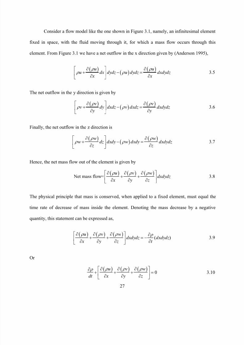
8/22/2019 Open Canopy Wind With Parapets
http://slidepdf.com/reader/full/open-canopy-wind-with-parapets 51/275
27
Consider a flow model like the one shown in Figure 3.1, namely, an infinitesimal element
fixed in space, with the fluid moving through it, for which a mass flow occurs through this
element. From Figure 3.1 we have a net outflow in the x direction given by (Anderson 1995),
u uu dx dydz u dydz dxdydz
x x
3.5
The net outflow in the y direction is given by
v vv dy dxdz v dxdz dxdydz
y y
3.6
Finally, the net outflow in the z direction is
w ww dz dxdy w dxdy dxdydz
z z
3.7
Hence, the net mass flow out of the element is given by
Net mass flow=
u v wdxdydz
x y z
3.8
The physical principle that mass is conserved, when applied to a fixed element, must equal the
time rate of decrease of mass inside the element. Denoting the mass decrease by a negative
quantity, this statement can be expressed as,
( )
u v wdxdydz dxdydz
x y z t
3.9
Or
0
u v w
dt x y z
3.10
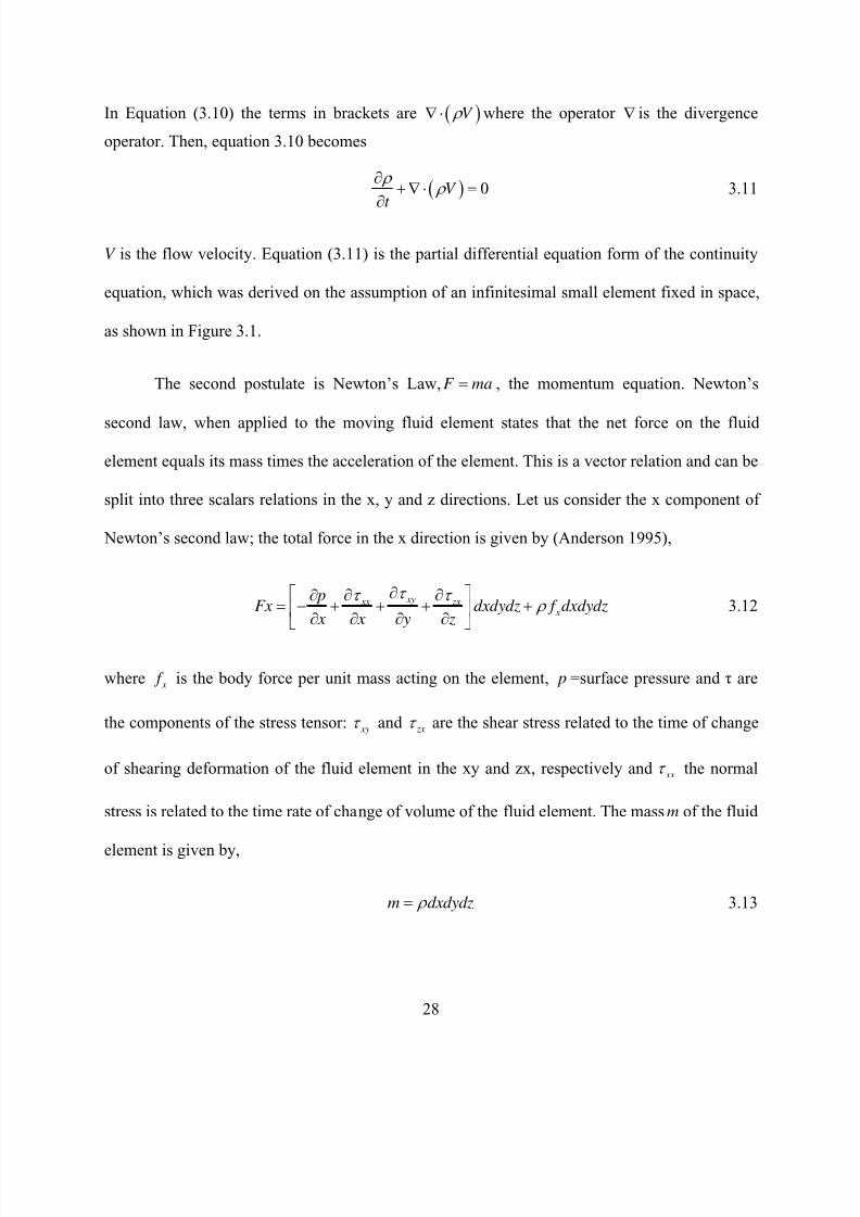
8/22/2019 Open Canopy Wind With Parapets
http://slidepdf.com/reader/full/open-canopy-wind-with-parapets 52/275
28
In Equation (3.10) the terms in brackets are V where the operator is the divergence
operator. Then, equation 3.10 becomes
0V t
3.11
V is the flow velocity. Equation (3.11) is the partial differential equation form of the continuity
equation, which was derived on the assumption of an infinitesimal small element fixed in space,
as shown in Figure 3.1.
The second postulate is Newton’s Law, F ma , the momentum equation. Newton’s
second law, when applied to the moving fluid element states that the net force on the fluid
element equals its mass times the acceleration of the element. This is a vector relation and can be
split into three scalars relations in the x, y and z directions. Let us consider the x component of
Newton’s second law; the total force in the x direction is given by (Anderson 1995),
xy xx zx x
pFx dxdydz f dxdydz
x x y z
3.12
where x f is the body force per unit mass acting on the element, p =surface pressure and τ are
the components of the stress tensor: xy
and zx are the shear stress related to the time of change
of shearing deformation of the fluid element in the xy and zx, respectively and xx the normal
stress is related to the time rate of change of volume of the fluid element. The mass m of the fluid
element is given by,
m dxdydz 3.13

8/22/2019 Open Canopy Wind With Parapets
http://slidepdf.com/reader/full/open-canopy-wind-with-parapets 53/275
29
Since we are following a moving fluid element, the rate of change with respect to time in the x
direction is given by,
x
Dua Dt 3.14
Combining equations (3.12), (3.13) and (3.14), we can obtain the x component of the momentum
equation for a viscous flow. The x, y and z components are the components of the momentum
equations (Anderson 1995).
yx xx zx
x
Du p
f Dt x x y z
3.15
xy yy zy
y
Dv p f
Dt y x y z
3.16
yz xz zz z
Dw p f
Dt z x y z
3.17
The partial differential equations were obtained from an application of the fundamental physical
principle to an infinitesimal fluid element. These are scalar equations and are called the Navier-
Stokes equations. These equations are (Anderson 1995),
yx xx zx
x
u puV f
t x x y z
3.18a
xy yy zy
y
v pvV f
t y x y z
3.18b
yz xz zz
z
w pwV f
t z x y z
3.18c
8/22/2019 Open Canopy Wind With Parapets
http://slidepdf.com/reader/full/open-canopy-wind-with-parapets 54/275
30
For virtually all practical aerodynamics problems, Stokes in 1845 obtained the constitutive
conditions in the form (Anderson 1995)
( ) 2 xx
uV
x
3.19a
( ) 2 yy
vV
y
3.19b
( ) 2 zz
w
V z
3.19c
xy yx
v u
x y
3.19d
xz zx
u w
z x
3.19e
yz zy
w v
y z
3.19f
where is the molecular viscosity coefficient and is the second viscosity coefficient. Stokes
made the hypothesis that2
3 . Substituting (3.19) into (3.18) we obtain the complete Navier-
Stokes equations in conservation form. In the CFD literature, a “Navier-Stokes solution” means a
solution of a viscous flow problem using the full governing equations. This includes the solution
for the momentum, energy and mass equations. They are a system of nonlinear partial
8/22/2019 Open Canopy Wind With Parapets
http://slidepdf.com/reader/full/open-canopy-wind-with-parapets 55/275
31
differential equations, and hence are difficult to solve analytically, with the consequence that no
general closed form solution exist to these equations at present.
The third postulate states that the energy is conserved. The first law of thermodynamics
states that when applied to the flow model of a fluid element moving with the flow, the rate of
change of energy inside the fluid element is equal to the heat into the element, plus the rate of
work done on the element due to body and surface forces. The rate of doing work by a force
exerted on a moving body is equal to the product of the force and the component of velocity in
the direction of the force.
Finally, a numerical method and a strategy for dividing the flow domain into cells or
elements must be selected. Many different gridding strategies exist, including structured,
unstructured, hybrid, composite, and overlapping grids. The most common choices of a
numerical method are finite difference, finite volume, finite element, and spectral methods
(Zingg 1999).
The most common finite difference representations of derivatives are based on Taylor’s
series expansions. The majority of the partial differential equations on the governing equations
can be replaced by a system of algebraic difference equations for the dependent variables of a
difference equation. Finite volume methods have become very popular in CFD as a result of two
major advantages: First, they ensure that the discretization of the governing equations is
conservative and second, the volume methods do not require transformations in order to be
applied to irregular meshes. The basic idea of the finite-volume method is to satisfy the integral
form of the conservation law to some degree of approximation for many continuous control
volumes, which cover the domain of interest. For this research, the finite volume method is used

8/22/2019 Open Canopy Wind With Parapets
http://slidepdf.com/reader/full/open-canopy-wind-with-parapets 56/275
32
(as implemented by the software developer), to satisfy the conservation law to some degree of
approximation for contiguous control volumes, which cover the domain of interest.
3.2 EFD.Lab program description
The wind flow on an open canopy structure with parapets can be represented and
modeled with the use of CFD. The specific CFD software used in this research is named
EFD.Lab (Engineering Fluid Dynamics), developed by Flomerics Inc. (Flomerics 2009).
EFD.Lab solves the Navier-Stokes equations, which include the formulations of mass,
momentum and energy conservation laws for fluid flows. The equations are supplemented by
fluid state equations defining the nature of the fluid and by empirical dependencies of fluid
density, viscosity and thermal conductivity on temperature (Flomerics 2009).
EFD.Lab solves the governing equations using the finite volume method (FVM) on a
prismatic rectangular computational mesh drawn in a 3D Cartesian coordinate system with the
planes orthogonal to its axes. To improve the results, the mesh is refined locally at the solid/fluid
interface. Turbulence is incorporated by means of turbulent intensity and turbulent length
parameters, which were obtained from the wind tunnel and used in the CFD computations in
order to emulate the wind tunnel conditions.
3.3 CFD model
The initial computational mesh used for the simulation is created in a prismatic domain,
as shown in Figure 3.2. The domain dimensions assumed in this initial example are 300 ft (91.4
m) in the x direction, 85 ft (25.9 m) in the z direction, and 80 ft (24.4 m) in the y direction. The
surface area on the left is defined as the inlet boundary, in which it is possible to introduce the

8/22/2019 Open Canopy Wind With Parapets
http://slidepdf.com/reader/full/open-canopy-wind-with-parapets 57/275
33
non-uniform values of a wind profile. The specific wind profile adopted in the first model
investigated in this research is a power law (as defined by ASCE 7 05),
1/( ) ( )( )ref
ref
zV z V z
z
This velocity profile has been investigated for the specific wind tunnel used in the research at
Universidad Nacional del Nordeste (UNNE) in Resistencia, Argentina, and a value of 1/ =0.24
is recommended by the researchers of that wind tunnel (De Bortoli et al. 2002). The exponent
1/ depends on the surface roughness and on the wind speed averaging time.ref
z is the
reference height, namely 10 m (32.8 ft). ( )ref V z is the velocity of reference at the height of
reference.
The simulation of a wind flow on a canopy requires the definition of a flow model and an
element mesh; each one has been considered in order to identify a mesh providing acceptable
results. Our first model considered is shown in Figure 3.2, in which the incoming flow has a
velocity profile which follows the power law. Different velocities on the left inlet entrance of
Figure 3.2 indicate that a wind profile using the power law was used as a wind velocity input.
The canopy induces significant changes to the flow, and the program calculates wind pressures
and Cp values on the model surfaces.

8/22/2019 Open Canopy Wind With Parapets
http://slidepdf.com/reader/full/open-canopy-wind-with-parapets 58/275
34
Figure 3.2: Computational domain for Model #1, with boundary definition and laminar
wind profile. The inlet condition is defined in the plane on the left.
EFD.Lab determines for external flows, the boundary conditions for all the boundaries of
the computational domain. The boundary conditions on any CFD problem define the solutions to
be obtained from the governing equations. In this particular model, the inlet surface has been
defined as mentioned before, a power law wind profile, with different wind velocities specified
through the height. The bottom boundary condition is automatically defined based on surface
roughness. The outlet boundary is defined as away from the surface boundary as possible,
simulating the real physical boundary condition. The rest of the boundaries assume a zero
relative velocity between the surface and the fluid immediately at the surface. This is called the
no-slip condition at the surface for a viscous flow.

8/22/2019 Open Canopy Wind With Parapets
http://slidepdf.com/reader/full/open-canopy-wind-with-parapets 59/275
35
A second computational model, named Model #2, with the same mesh configuration as
Model #1, was also built, in which a uniform flow was assumed, i.e. a uniform velocity profile in
height was assumed at the inlet boundary (see Figure 3.3). Although the inlet conditions between
a power law and a uniform velocity profile are very different, in the present case in which the
canopy is a thin body located at a given distance from the terrain, the results in terms of
pressures acting on the canopy are remarkably similar. The reasons for this similarity are that the
canopy is located away from the turbulence generated at the ground level, and the pressures are
dominated by the pressures and velocities that occur at the canopy height. Such similarity is only
specific of this case and does not occur in enclosed structures.
Figure 3.3: Computational domain for Model #2, without boundary definition and uniform
wind profile.
To investigate the sensitivity of the solution to changes in the number of elements
adopted, the laminar model was considered. A third computational model (see Figure 3.4),
named Model #3 was also created. This model has a smaller computational domain in which

8/22/2019 Open Canopy Wind With Parapets
http://slidepdf.com/reader/full/open-canopy-wind-with-parapets 60/275
36
laminar flow was assumed with a constant velocity profile in height at the inlet boundary. The
domain dimensions assumed in this initial example are 150 ft (45.7 m) in the x direction, 85 ft
(25.9 m) in the z direction, and 80 ft (24.4 m) in the y direction. This computational model was
created to verify if similar results can be obtained with a smaller computational domain and
number of fluid cells compared to the computational domain on Model #2 and Model #1.
Figure 3.4: Computational domain for Model #3, without boundary definition and uniform
wind profile.
The results from the initial computational domain, Model #1, with the use of the inlet
boundary layer calculated with the power law, were compared against a similar domain in terms
of geometry and number of fluid cells. The number of fluid cells generated for Model #1 and
Model #2 was 303,123. The domain for Model #3 generated a number of cells of 54,954. The
computational time on a personal computer was drastically reduced from 3 hours and 27 minutes
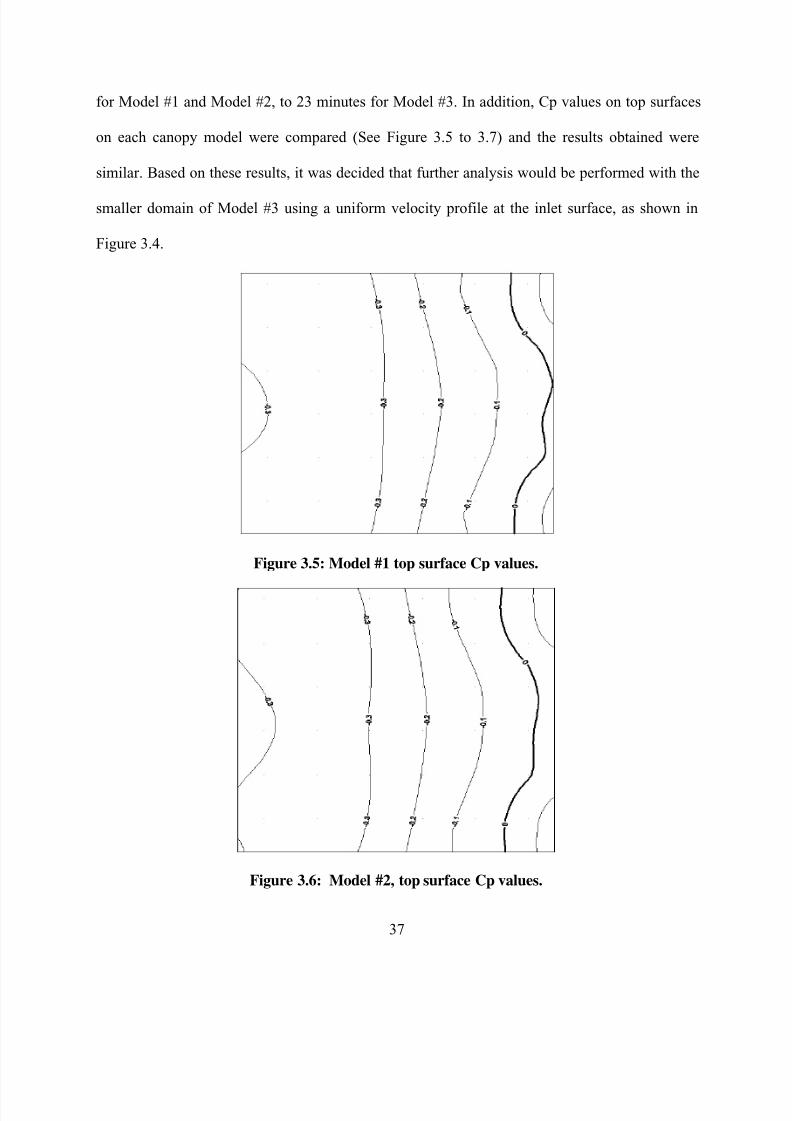
8/22/2019 Open Canopy Wind With Parapets
http://slidepdf.com/reader/full/open-canopy-wind-with-parapets 61/275
37
for Model #1 and Model #2, to 23 minutes for Model #3. In addition, Cp values on top surfaces
on each canopy model were compared (See Figure 3.5 to 3.7) and the results obtained were
similar. Based on these results, it was decided that further analysis would be performed with the
smaller domain of Model #3 using a uniform velocity profile at the inlet surface, as shown in
Figure 3.4.
Figure 3.5: Model #1 top surface Cp values.
Figure 3.6: Model #2, top surface Cp values.

8/22/2019 Open Canopy Wind With Parapets
http://slidepdf.com/reader/full/open-canopy-wind-with-parapets 62/275
38
Figure 3.7: Model #3, top surface Cp values.
The significance of velocity in the model and in real situations is not self-evident and
needs some clarification. The sustained wind velocity used for analysis on Model #2 and Model
#3 was obtained from the wind velocity in Model #1, with the use of the power law formula. The
wind speed velocity calculation with an hourly wind speed of 96 mph (145 mph 3 sec gust wind
speed, same as ASCE 7-05 basic wind speed for Puerto Rico) was obtained using Figure C6-2, in
the ASCE 7-05 Commentary (ASCE 2005).
1/ 1/4.1612( ) ( )( ) 96 ( ) 75
32.8ref
ref
z ft V z Vz mph mph
z ft
3.21
ref Vz hourly wind speed wind speed (mph), z mean roof height (ft),
ref z reference height =
32.8 ft (10 m), 1/ power law exponent = 1/4.16 = 0.24 for open terrain on the UNNE wind
tunnel.
This result is based on the power law and the result is the hourly wind speed at 12 ft
averaged over one hour. The averaged one hour wind speed is commonly used as a reference
wind speed in wind tunnel simulations. The hourly wind speed obtained will be used in the CFD
simulations for Model #2 and Model #3.

8/22/2019 Open Canopy Wind With Parapets
http://slidepdf.com/reader/full/open-canopy-wind-with-parapets 63/275
39
The wind speed in Model #1 at the canopy roof height was approximately 75 mph. The
same wind velocity of 75 mph, but sustained, instead of a wind profile calculated by the power
law, was applied to Model #2 and Model #3. This means that the same wind velocity was applied
on all investigated models at open canopy height. The results for laminar (Figure 3.5) and for
uniform velocity flow (Figure 3.6) are virtually identical in terms of values and distributions.
Based on the agreement and on the significant differences in computer time required, it was
decided that the detailed investigations and comparisons with wind tunnel would be done using
uniform velocity flow. Regarding the use of a different number of cell elements in the uniform
velocity flow (Figures 3.6 and 3.7), some small differences were obtained in the results. The area
of exposure of both models against the wind at the same canopy heights is similar. Further
analysis was performed with the smaller domain of Model #3, using a uniform velocity profile at
the inlet surface. The CFD Reynolds number calculated for the simulation is 8.52x10⁷.
The CFD software yields results of wind pressures on the external (top and bottom)
surfaces of the structure. In this case, a wind velocity similar to those specified by design codes
has been adopted, with an hourly wind speed of 33.5 m/s (75 mph) for all simulations. This
sustained wind speed is equivalent to 64.8 m/s (145 mph) 3 second gust wind speed, as required
by ASCE 7-05 for Puerto Rico. Within the context of this research, CFD simulations were
extremely useful to identify and define the geometric characteristics of the canopies to be
investigated prior to the construction of physical models that were tested in a wind tunnel
facility. Preliminary investigations allowed the identification of the high-pressure areas, which
were in turn used to specify the location of the wind pressure taps that were used in the small
scale models.

8/22/2019 Open Canopy Wind With Parapets
http://slidepdf.com/reader/full/open-canopy-wind-with-parapets 64/275
40
The initial geometry of the canopy analyzed consists of a 7.6 m (25 ft) x 7.6m (25ft) with
a 1.2m (4ft) parapet. The roof height is located at 3.6m (12ft). The proposed geometry was
decided after comparing photographs and visits through many existing gas stations in Puerto
Rico. The proposed geometry is very common and used in many gas stations in Puerto Rico.
The mesh cells sides used on the program are orthogonal to the specified axes on the
coordinate system. The mesh can be automatically created using a mesh generator, but the mesh
in this simulation was specified so that it could be refined on the exposed surfaces. Further sub-
meshing was assigned for refinement on all exposed surfaces. Refer to Figure 3.8 and Figure 3.9
for meshing and sub-meshing images.
Figure 3.8: Computational domain and meshing used in Model #3.
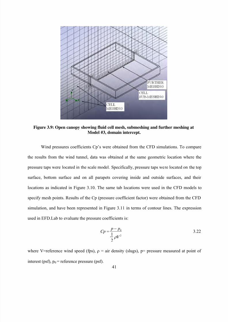
8/22/2019 Open Canopy Wind With Parapets
http://slidepdf.com/reader/full/open-canopy-wind-with-parapets 65/275
41
Figure 3.9: Open canopy showing fluid cell mesh, submeshing and further meshing at
Model #3, domain intercept.
Wind pressures coefficients Cp’s were obtained from the CFD simulations. To compare
the results from the wind tunnel, data was obtained at the same geometric location where the
pressure taps were located in the scale model. Specifically, pressure taps were located on the top
surface, bottom surface and on all parapets covering inside and outside surfaces, and their
locations as indicated in Figure 3.10. The same tab locations were used in the CFD models to
specify mesh points. Results of the Cp (pressure coefficient factor) were obtained from the CFD
simulation, and have been represented in Figure 3.11 in terms of contour lines. The expression
used in EFD.Lab to evaluate the pressure coefficients is:
0
21
2
p pCp
V
3.22
where V=reference wind speed (fps), = air density (slugs), p= pressure measured at point of
interest (psf), p0 = reference pressure (psf).

8/22/2019 Open Canopy Wind With Parapets
http://slidepdf.com/reader/full/open-canopy-wind-with-parapets 66/275
42
The CFD model with the location of the pressure taps has is shown in Figure 3.12. As
mentioned before, the pressure taps are at the same locations as in the model tested at the wind
tunnel. Results from those simulations will be reported in Chapter 6 of this dissertation.
Figure 3.10: Pressure tap locations on top, bottom and parapet surfaces used for
CFD and wind tunnel scale model.

8/22/2019 Open Canopy Wind With Parapets
http://slidepdf.com/reader/full/open-canopy-wind-with-parapets 67/275
43
Figure 3.11: Location of pressure taps and measured wind pressures on the top surface.
Wind direction acting from the right (0 degrees).
Figure 3.12: Model pressure taps on the canopy model.
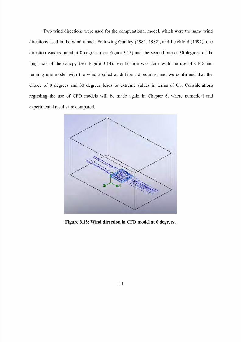
8/22/2019 Open Canopy Wind With Parapets
http://slidepdf.com/reader/full/open-canopy-wind-with-parapets 68/275
44
Two wind directions were used for the computational model, which were the same wind
directions used in the wind tunnel. Following Gumley (1981, 1982), and Letchford (1992), one
direction was assumed at 0 degrees (see Figure 3.13) and the second one at 30 degrees of the
long axis of the canopy (see Figure 3.14). Verification was done with the use of CFD and
running one model with the wind applied at different directions, and we confirmed that the
choice of 0 degrees and 30 degrees leads to extreme values in terms of Cp. Considerations
regarding the use of CFD models will be made again in Chapter 6, where numerical and
experimental results are compared.
Figure 3.13: Wind direction in CFD model at 0 degrees.
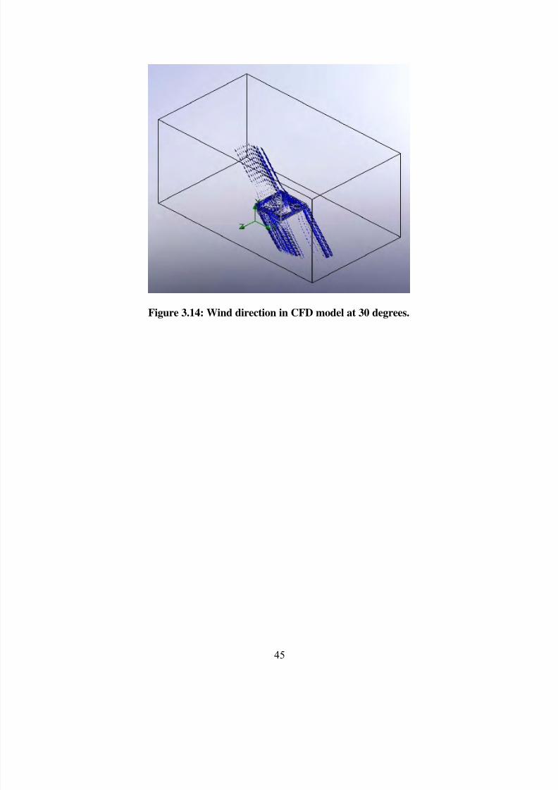
8/22/2019 Open Canopy Wind With Parapets
http://slidepdf.com/reader/full/open-canopy-wind-with-parapets 69/275
45
Figure 3.14: Wind direction in CFD model at 30 degrees.
8/22/2019 Open Canopy Wind With Parapets
http://slidepdf.com/reader/full/open-canopy-wind-with-parapets 70/275
46
CHAPTER 4. WIND TUNNEL TESTING
4.1 General features of wind tunnel studies
The use of wind tunnels to aid in civil engineering, structural design and planning has been
increasing in recent years. The purpose of wind tunnel tests is to provide designers with
information on local wind parameters, and wind loads having an accuracy far exceeding that
which can be obtained from predictions based on other less expensive means such as theory,
numerical analysis, and consulting (Liu 1991).
Some structures warrant a wind tunnel test, like skyscrapers, large structures, constructions
having unusual shapes or major structures located in special locations. Examples of special
locations are those affected by topographical features, such as hills, cliffs or valleys. In these
situations, the use of wind tunnel tests is used to improve the final design. Failure to conduct
tests or investigate using the wind tunnel may result in an unsafe design.
A wind tunnel model test conducted in the United States may approximately cost in the order
of forty thousand dollars, so that most companies cannot afford a wind tunnel test for every
structure to be analyzed. A wind tunnel test cannot be financially justified, unless the expected
savings from such a test are far greater that the cost of conducting it. Safety in most of the cases
is not the motivation for wind tunnel tests. Savings in cladding are the primary motivation in
terms of analyzing structures with complex geometries. In several cases, wind tunnel testing can
produce thousands of dollars in savings when actual wind pressures can be obtained from it.
Numerous criteria exist to categorize wind tunnels. According to the flow circuit, a tunnel
may be classified as either an open or closed circuit tunnel. An open circuit tunnel is normally a

8/22/2019 Open Canopy Wind With Parapets
http://slidepdf.com/reader/full/open-canopy-wind-with-parapets 71/275
47
straight structure. Air is drawn into the tunnel from a funnel-shape intake at one end of the
tunnel, and the air exits the tunnel through a funnel shape outlet. The enlarged cross-sectional
areas at the two ends prevent undesirable strong winds from being generated outside the tunnel
near the inlet or outlet. The closed circuit type is a recirculation loop. It may occupy a small
space if the loop is vertical. Advantages of closed circuit tunnels are, (1) they do not cause
undesirable winds in laboratories housing the wind tunnels; (2) they generate less noise. Both
open and closed circuit tunnels are often used for testing structural models. The tunnel used in
this investigation, was an open circuit tunnel at UNNE.
A boundary layer wind tunnel must have a test section that is sufficiently long to generate a
thick vertical boundary layer, sufficiently high so that the boundary layer generated will not
touch the tunnel ceiling and sufficiently wide so that neighboring structures and topographical
features can be incorporated into the model. Furthermore, the blockage ratio, which is the ratio of
the cross sectional area of the model blocking the flow and the cross sectional area of the tunnel
test section, must be less than one tenth. These requirements necessitate rather large tunnels. The
boundary layer tunnels used in commercial testing of structural models normally have a
minimum width of 2.4 m (8ft), minimum height of 1.5 m (5 ft), and a minimum length of 10 m
(33 ft), all measures referring to test sections.
To facilitate the rapid growth of a vertical boundary layer along the tunnel test section,
roughness elements must be placed on the tunnel floor, and additional devices, such as spires,
must be installed upstream. The roughness and the spires must be designed to produce the type
of velocity profile and the type of turbulence similar to that encountered by the prototype
structure. Typically, the model tested in a wind tunnel is placed on a turntable so that it can be
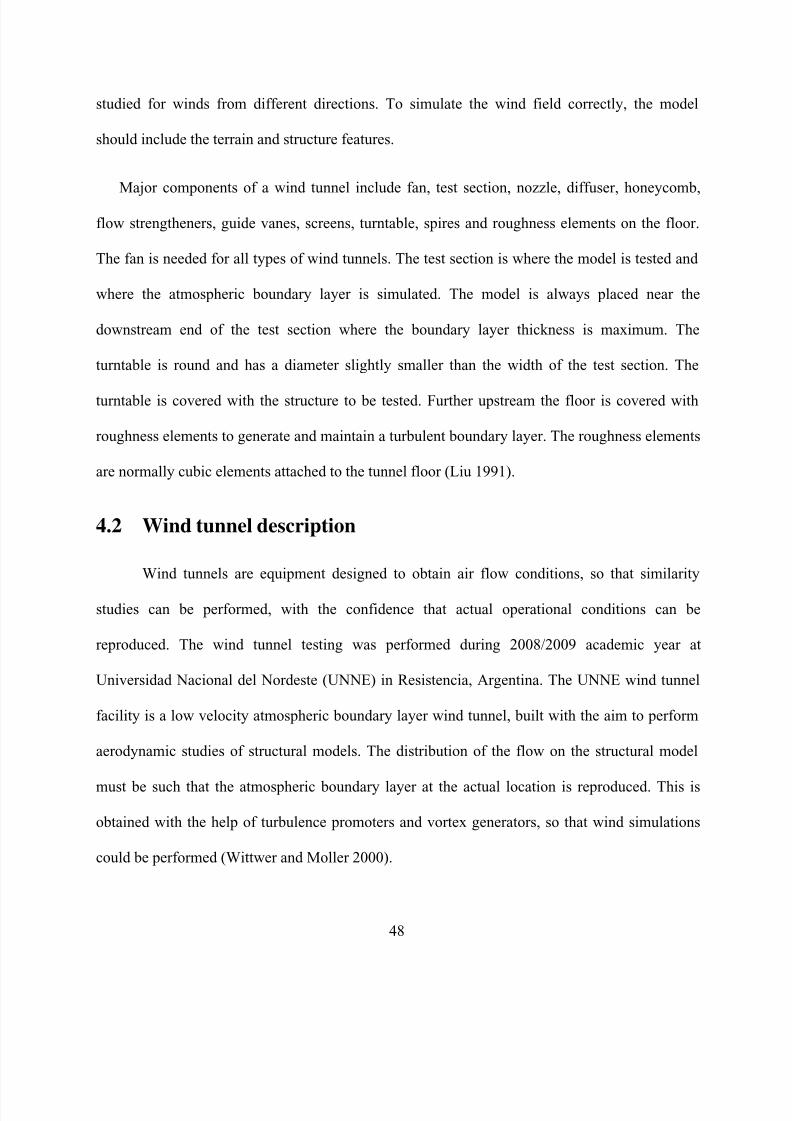
8/22/2019 Open Canopy Wind With Parapets
http://slidepdf.com/reader/full/open-canopy-wind-with-parapets 72/275
48
studied for winds from different directions. To simulate the wind field correctly, the model
should include the terrain and structure features.
Major components of a wind tunnel include fan, test section, nozzle, diffuser, honeycomb,
flow strengtheners, guide vanes, screens, turntable, spires and roughness elements on the floor.
The fan is needed for all types of wind tunnels. The test section is where the model is tested and
where the atmospheric boundary layer is simulated. The model is always placed near the
downstream end of the test section where the boundary layer thickness is maximum. The
turntable is round and has a diameter slightly smaller than the width of the test section. The
turntable is covered with the structure to be tested. Further upstream the floor is covered with
roughness elements to generate and maintain a turbulent boundary layer. The roughness elements
are normally cubic elements attached to the tunnel floor (Liu 1991).
4.2 Wind tunnel description
Wind tunnels are equipment designed to obtain air flow conditions, so that similarity
studies can be performed, with the confidence that actual operational conditions can be
reproduced. The wind tunnel testing was performed during 2008/2009 academic year at
Universidad Nacional del Nordeste (UNNE) in Resistencia, Argentina. The UNNE wind tunnel
facility is a low velocity atmospheric boundary layer wind tunnel, built with the aim to perform
aerodynamic studies of structural models. The distribution of the flow on the structural model
must be such that the atmospheric boundary layer at the actual location is reproduced. This is
obtained with the help of turbulence promoters and vortex generators, so that wind simulations
could be performed (Wittwer and Moller 2000).

8/22/2019 Open Canopy Wind With Parapets
http://slidepdf.com/reader/full/open-canopy-wind-with-parapets 73/275
49
Figure 4.1: View the UNNE wind tunnel facility. (Photograph by the Author)
The facility is an open circuit tunnel with a length of 22.8 m (74.8 ft), the testing chamber
being a rectangular section of 2.4 m (7.87 ft) width and 1.8 m (5.9 ft) in height and uses a 2.25 m
diameter (7.38 ft) fan with a 92 kW motor. The maximum wind velocity that may be obtained in
this tunnel is 25 m/s (55.9 mph) when the testing section is empty (the section is empty when
there is no model in the testing chamber). Further details regarding this wind facility are given by
Wittwer and Möller (2000).
All models were tested under a wind simulation corresponding to a suburban area. The
simulation of the natural wind on the atmospheric boundary layer was performed by means of
the Counihan and Standen methods with velocity distributions defined as ground covered by
several closely spaced obstacles in forest or urban territory (Wittwer and Moller 2000). The
Counihan and Standen methods are techniques developed to thicken boundary layers on wind
8/22/2019 Open Canopy Wind With Parapets
http://slidepdf.com/reader/full/open-canopy-wind-with-parapets 74/275
50
tunnels. These techniques are generally known as roughness, barrier and mixing-device methods
(Natalini et al. 1998). Surface roughness was obtained on 17 m (55.7 ft) test floor section with
prismatic 30x30x22 mm (1.18x1.18x.89 in) elements, 80 mm (3.14 in) apart. The choice of
element size and packing density was based on the works of Counihan, Fang and Sill, Gartshore
and Cross (Natalini et al. 1998).
Representative values of power law exponent 1/ 0.24 and the roughness length
parameter 0 0.7 z m were adopted in order to obtain a scale of 1:500, a usual scale in
simulations. Consequently, the design value in the wind tunnel for the specified scale is
0 1.4 z mm . The same suburban terrain exponent was used on the CFD simulation. The
suburban terrain condition corresponds to open terrain with scattered obstructions having heights
of less than 9.1 m (30 ft). According to the ASCE 7-05, it corresponds to Exposure B. In order to
obtain a boundary layer depth of 1.3 m artificial simulation methods were applied. This
technique called natural simulation produces simulation scales higher than 1:500, and it requires
the use of long wind tunnels. The simulation hardware consisted of two modified Irwin’s spires,
as shown in Figure 4.2 and 4.3. Figure 4.4 shows the tunnel plan at UNNE.

8/22/2019 Open Canopy Wind With Parapets
http://slidepdf.com/reader/full/open-canopy-wind-with-parapets 75/275
51
Figure 4.2: Typical Irwin spires used on the UNNE wind tunnel.
Figure 4.3:View the UNNE surface roughness and Irwin spires. (Photograph by the
Author)

8/22/2019 Open Canopy Wind With Parapets
http://slidepdf.com/reader/full/open-canopy-wind-with-parapets 76/275
52
Figure 4.4: Wind tunnel plan at UNNE (reproduced from Wittwer and Moller 2000).
In this way, a part-depth boundary layer simulation of neutrally stable atmosphere was
obtained. Mean velocities, when fitted to a potential law, with an exponent of 0.24 obtained at
UNNE are shown on Figure 4.5.
Figure 4.5: Mean velocity profiles at the UNNE wind tunnel (Wittwer and Moller 2000).
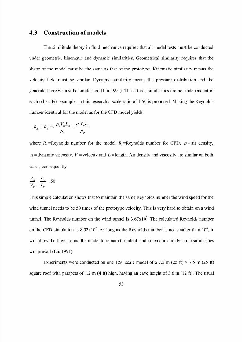
8/22/2019 Open Canopy Wind With Parapets
http://slidepdf.com/reader/full/open-canopy-wind-with-parapets 77/275
53
4.3 Construction of models
The similitude theory in fluid mechanics requires that all model tests must be conducted
under geometric, kinematic and dynamic similarities. Geometrical similarity requires that the
shape of the model must be the same as that of the prototype. Kinematic similarity means the
velocity field must be similar. Dynamic similarity means the pressure distribution and the
generated forces must be similar too (Liu 1991). These three similarities are not independent of
each other. For example, in this research a scale ratio of 1:50 is proposed. Making the Reynolds
number identical for the model as for the CFD model yields
p p pm m mm p
m p
V LV L R R
where Rm=Reynolds number for the model, R p=Reynolds number for CFD, air density,
dynamic viscosity, V velocity and L length. Air density and viscosity are similar on both
cases, consequently
50 pm
p m
LV V L
This simple calculation shows that to maintain the same Reynolds number the wind speed for the
wind tunnel needs to be 50 times of the prototype velocity. This is very hard to obtain on a wind
tunnel. The Reynolds number on the wind tunnel is 3.67x10⁶. The calculated Reynolds number
on the CFD simulation is 8.52x10⁷. As long as the Reynolds number is not smaller than 10
4, it
will allow the flow around the model to remain turbulent, and kinematic and dynamic similarities
will prevail (Liu 1991).
Experiments were conducted on one 1:50 scale model of a 7.5 m (25 ft) × 7.5 m (25 ft)
square roof with parapets of 1.2 m (4 ft) high, having an eave height of 3.6 m.(12 ft). The usual

8/22/2019 Open Canopy Wind With Parapets
http://slidepdf.com/reader/full/open-canopy-wind-with-parapets 78/275
54
scale for wind tunnel testing of open structures varies from 1:50 to 1:100. In this particular
research, a scale of 1:50 was chosen in order to install all the PVC tubes to be connected to the
testing instruments without any interference.
First, experiments were carried out without parapets in order to compare with other wind
tunnel results available in the open literature. Wind load coefficients were measured under wind
blowing at angles of 0º and 30º relative to one of the symmetry axis, since, as demonstrated by
Gumley (1981, 1982) and Letchford et al. (1992) among others, these directions produce the
most severe loads on planar canopy roofs with no parapets. In the absence of additional
information, it was expected that such angles would still be relevant for canopies with parapets.
The roof of the model and the parapets were made with a 2 mm thick aluminum plate,
and the columns with a 2.5 mm diameter steel rod. As the models have two axes of symmetry,
only a quarter of the roof model was instrumented with pressure taps in place, thus reducing the
number of tubes needed. In addition, all the tubes were led towards the farthest corner, where
they formed a bundle that went into a horizontal pipe through which they went away from the
model to finally go under the floor. In this way, the scale distortion in both columns and roof
thickness and the possible interference of the tubes upon the measurements were minimized. The
model is shown in Figures 4.6 to 4.8.
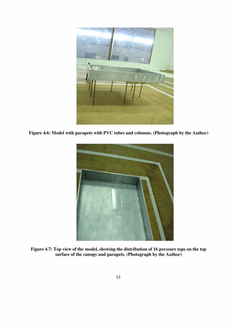
8/22/2019 Open Canopy Wind With Parapets
http://slidepdf.com/reader/full/open-canopy-wind-with-parapets 79/275
55
Figure 4.6: Model with parapets with PVC tubes and columns. (Photograph by the Author)
Figure 4.7: Top view of the model, showing the distribution of 16 pressure taps on the top
surface of the canopy and parapets. (Photograph by the Author)

8/22/2019 Open Canopy Wind With Parapets
http://slidepdf.com/reader/full/open-canopy-wind-with-parapets 80/275
56
Figure 4.8: Distribution of pressure taps on the model with bundle of tubes and columns.
(Photograph by the Author)
Sixteen pressure taps were spread on the roof and twenty on the parapets. The specific
locations of the taps were influenced by the previous computational results which indicated, and
suggested places of special interest in terms of pressure values. Figure 4.9 shows the position of
the pressure taps on the top surface of the model and Figure 4.10 shows the model placed in the
turntable. The turntable is a round table of 1.5 m (4.9 ft) of width, which is rotated during the
wind test in order to obtain the desired wind pressures.
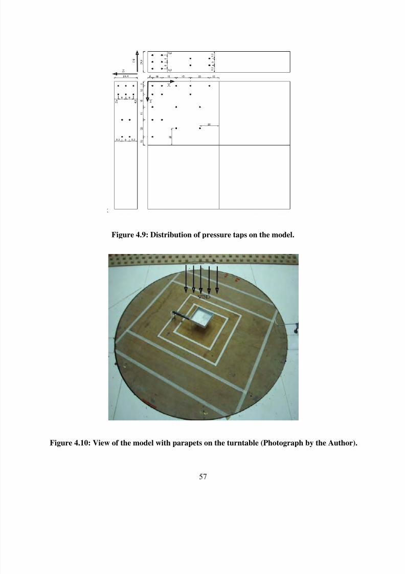
8/22/2019 Open Canopy Wind With Parapets
http://slidepdf.com/reader/full/open-canopy-wind-with-parapets 81/275
57
Figure 4.9: Distribution of pressure taps on the model.
Figure 4.10: View of the model with parapets on the turntable (Photograph by the Author).

8/22/2019 Open Canopy Wind With Parapets
http://slidepdf.com/reader/full/open-canopy-wind-with-parapets 82/275
58
4.4 Instrumentation
Pressures were measured using a differential pressure electronic transducer. The brand
used in this tunnel is Micro Switch Honeywell 163 PC (Figure 4.11). The transducer converts the
pressure differences from the model and the reference static pressures, to differences in voltage.
Figure 4.11: View of the pressure electronic transducer Honeywell 163PC. (Photograph by
the Author)
A sequential switch Scanivale 48 D9-1/2, which was driven by means of a CTLR2 / S2-
S6 solenoid controller, connected the pressure taps to the transducer through PVC tubes of 1.5
mm internal diameter and 650 mm in length (Figure 4.12). The Scanivale system is the only
working system available in this tunnel. It has some disadvantages in the sense that
measurements cannot be taken simultaneously but should be obtained following a sequence.
Each PVC tube connected to the Scanivale is connected to a pressure tap on the scale model. For
this experiment, each pressure tap data was acquired once at a time following a numerical order.

8/22/2019 Open Canopy Wind With Parapets
http://slidepdf.com/reader/full/open-canopy-wind-with-parapets 83/275
59
Figure 4.12: View of the Scanivale 48 D9-1/2 w/PVC tubes (Photograph by the Author).
No resonance problems were detected for tubes of that length. Therefore, restrictors for
the tubes were not used for filtering. When a fluctuating signal flows through the tubes in order
to reach the Scanivale, verification that the signal is not amplified or with distortion is done
through comparison with previous results. Those signals go to the DC transducer output and
were read with the aid of a Keithley 2000 digital multimeter. The integration time operation rate
of the A/D converter was set to produce mean values over 15 seconds of time integration (Figure
4.13). The multimeter was configured to read and store the values every 0.6 seconds, and every
25 readings and average are recorded every 15 seconds. This procedure can obtain variances in
the order of +/- 0.02 of the pressure coefficient.

8/22/2019 Open Canopy Wind With Parapets
http://slidepdf.com/reader/full/open-canopy-wind-with-parapets 84/275
60
Figure 4.13: View of the UNNE Keithley 2000 digital multimeter (Photograph by the
Author).
Simultaneously to the pressure measurements being taken on any of the roof surfaces, the
reference dynamic pressure, q ref , was measured at the eave’s height with a Pitot-Prandtl tube
connected to a Van Essen 2500 Betz differential micro-manometer of 1 Pa resolution (Figure
4.14). The probe stayed beside the model at a distance of about 0.70 m to avoid mutual
interference. The reference static pressure was obtained from the static pressure taps of the same
Pitot-Prandlt tube (Figure 4.15).

8/22/2019 Open Canopy Wind With Parapets
http://slidepdf.com/reader/full/open-canopy-wind-with-parapets 85/275
61
Figure 4.14: View of the Van Essen 2500 Betz differential micro manometer. (Photograph
by the Author)
Figure 4.15: View of the Pitot-Prandtl tube. (Photograph by the Author)
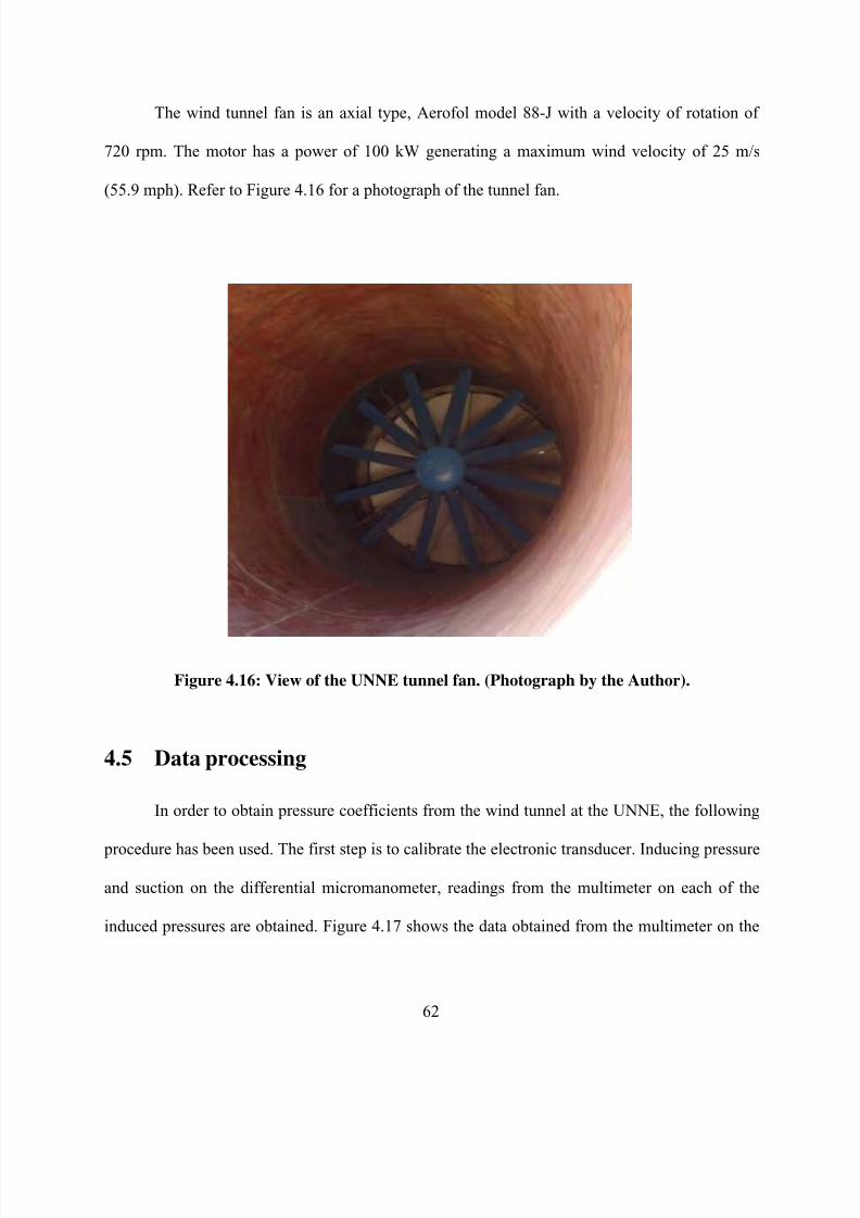
8/22/2019 Open Canopy Wind With Parapets
http://slidepdf.com/reader/full/open-canopy-wind-with-parapets 86/275
62
The wind tunnel fan is an axial type, Aerofol model 88-J with a velocity of rotation of
720 rpm. The motor has a power of 100 kW generating a maximum wind velocity of 25 m/s
(55.9 mph). Refer to Figure 4.16 for a photograph of the tunnel fan.
Figure 4.16: View of the UNNE tunnel fan. (Photograph by the Author).
4.5 Data processing
In order to obtain pressure coefficients from the wind tunnel at the UNNE, the following
procedure has been used. The first step is to calibrate the electronic transducer. Inducing pressure
and suction on the differential micromanometer, readings from the multimeter on each of the
induced pressures are obtained. Figure 4.17 shows the data obtained from the multimeter on the

8/22/2019 Open Canopy Wind With Parapets
http://slidepdf.com/reader/full/open-canopy-wind-with-parapets 87/275
63
model without parapets. The procedure is done at the beginning of the test and at the end to
verify that there were no sudden pressure changes that can affect the measured data.
Figure 4.17: Calibration data on model without parapets.
Figure 4.18: Photograph showing the author taking data from the wind tunnel test.
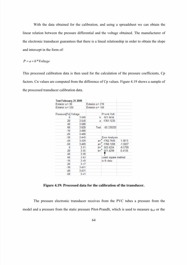
8/22/2019 Open Canopy Wind With Parapets
http://slidepdf.com/reader/full/open-canopy-wind-with-parapets 88/275
64
With the data obtained for the calibration, and using a spreadsheet we can obtain the
linear relation between the pressure differential and the voltage obtained. The manufacturer of
the electronic transducer guarantees that there is a lineal relationship in order to obtain the slope
and intercept in the form of:
*P a b Voltage
This processed calibration data is then used for the calculation of the pressure coefficients, Cp
factors. Cn values are computed from the difference of Cp values. Figure 4.19 shows a sample of
the processed transducer calibration data.
Figure 4.19: Processed data for the calibration of the transducer.
The pressure electronic transducer receives from the PVC tubes a pressure from the
model and a pressure from the static pressure Pitot-Prandlt, which is used to measure q ref or the

8/22/2019 Open Canopy Wind With Parapets
http://slidepdf.com/reader/full/open-canopy-wind-with-parapets 89/275
65
dynamic pressure of reference. This potential difference is measured with the digital multimeter.
This signal is fluctuating due to the fluctuation of the wind. As mentioned before, the multimeter
was configured to read and store the values every 0.6 seconds, and after 25 readings, an average
is recorded (every 15 seconds). Figure 4.20 shows the processed data after the transducer was
calibrated. The pressure difference, for example, is obtained using the previous equation:
* ( 1761.12 501.84*(3.504)) 2.664P a b Voltage Pa
Figure 4.20: Processed data for the pressure coefficient Cp.
The dynamic pressure of reference, q ref , is measured with the differential micromanometer. The
final pressure coefficient is the dynamic pressure/q ref . The net pressure coefficient (Cn) is the
difference between the external pressure coefficient and the internal pressure coefficient.
Appendix B through E shows the complete data sets, and the procedure with the calculated
values on spreadsheets. The results from the wind tunnel tests will be presented and discussed in
Chapter 6.

8/22/2019 Open Canopy Wind With Parapets
http://slidepdf.com/reader/full/open-canopy-wind-with-parapets 90/275
66
CHAPTER 5. AVAILABLE DESIGN CODE INFORMATION
5.1 General Code Information
Open structures have been designed and constructed in many countries for a number of
years. In each case, the designer follows national standards based on best practices. However,
little help is found with reference to the problem posed in this dissertation. For the sake of
completeness, the design of open structures according to current building codes has been
investigated during this research. Several design codes and standards are currently in use
worldwide, such as the Uniform Building Code (1997 Edition), the ASCE 7-05 standard, the
Eurocode, the Australian Code and the Japanese Code. Those were investigated to identify their
current design criteria for the design of open structures. First, American codes (the UBC 97 and
the ASCE 7-05) will be discussed in order to investigate current design criteria for the analysis of
open canopy structures with parapets. Next, we will mention other design codes used worldwide,
and whether they have available information in the design of open canopy structures with
parapets.
5.2 UBC 97
The Uniform Building Code, (1997 Edition) is a design code still in use in the West of
the United States, and it is also the required building code in use in Puerto Rico. The UBC 97 is
complemented in Puerto Rico with the use of the ASCE 7-05 for the calculation of wind
pressures. The Uniform Building code covers the design of many types of structures. The open
canopy structures will be included on what is called by the code, “unenclosed structures” as
defined by Section 1616.
8/22/2019 Open Canopy Wind With Parapets
http://slidepdf.com/reader/full/open-canopy-wind-with-parapets 91/275
67
The basic wind speed is the fastest mile wind speed associated with an annual probability
of occurrence of 0.02 measured at a point 33 feet above the ground for an exposure category C
(UBC 1997), as defined by Section 1618. Design wind pressures are defined on Section 1620.
Wind pressure for buildings and calculations are obtained in accordance to
e q s wP C C q I (UBC 20-1)
wheree
C Gust factor coefficient, as given in UBC Table 16-G,q
C = Pressure coefficient, as
given in UBC Table 16-H, w I Importance factor in UBC, Table 16-K, P Design wind
pressure, sq Wind stagnation pressure, as set forth in UBC Table 16-F.
The primary load resisting system of every structure shall be designed for the pressures
using UBC formula 20-1. Two primary methods, Method 1 (normal force method) and Method 2
(projected area method), are the two methods commonly used for the calculation of wind
pressures. No specific design procedure is available for the design of open structures with
parapets in the Uniform Building Code, 1997 edition.
5.3 ASCE 7-05
The American Society of Civil Engineers provisions, ASCE 7-05, provide three
procedures for the calculation of wind loads. Method 1 or the simplified procedure is discussed
in Section 6.4 of the ASCE document, Method 2, the analytical procedure is found in Section 6.5
of the document and Method 3, is the wind tunnel procedure which is described in Section 6.6.
The basic wind speed is the 3-second gust speed at 33 ft (10 m) above the ground in open
terrain. The basic wind speeds are specified in the ASCE wind maps in their Figure 6-1. In
8/22/2019 Open Canopy Wind With Parapets
http://slidepdf.com/reader/full/open-canopy-wind-with-parapets 92/275
68
Puerto Rico the basic 3-second gust wind is 145 mph. The wind speeds are assumed to be the
same for all horizontal directions.
Method 2, the analytical procedure on Section 6.5 describes the procedures for
determining the wind pressures. Method 1 cannot be used for the design of open structures due to
Section 6.4.1.1 item 3, which describes that it can only be used for enclosed structures.
Section 6.5.10 describes the formula for the calculation of the velocity pressure as follows:
2.00256 z z zt d q K K K V I (ASCE 6-15)
where z
K =velocity pressure exposure coefficient, defined in Section 6.5.6.6, zt
K =topographic
factor, defined in Section 6.5.7.2, d K =wind directionality factor, defined in Section 6.5.4.4,
V velocity from Figure 6-1, I Importance factor for the building or other structure which is
determined from Table 6-1.
Regarding exposure, for each wind direction being considered, the upwind exposure
category shall be based on ground surface roughness, which is determined from the natural
topography, vegetation or surrounding constructed facilities (ASCE 7-05). Surface roughness
categories are defined in Section 6.5.6.2. Surface roughness C is used for the wind tunnel
simulation and CFD model simulation. Gust effect factor is determined on section 6.5.8. For
rigid structures, one should use Section 6.5.8.1 and for flexible of dynamically sensitive
structures, Section 6.5.8.2.
Enclosure classifications are defined in Section 6.5.9 in such a way that all buildings shall
be classified as enclosed, partially enclosed or open. Section 6.5.13 covers the design of wind
loads for open buildings with monoslope, pitched or troughed roofs. Parapets shall be designed
as explained in Section 6.5.12.2.4. The ASCE 7-05 does not provide coefficients for structures

8/22/2019 Open Canopy Wind With Parapets
http://slidepdf.com/reader/full/open-canopy-wind-with-parapets 93/275
69
that combine both, open canopy and parapets in the same structure. No previous studies have
been done evaluating the proposed code coefficients.
5.4 IBC 2006
The most recent design code in the United States is the International Building Code, 2006
Edition. This code is used in the entire nation, and almost all the states are adopting it, or are in
the process of incorporating the code to their standards. The IBC 2006 makes reference to the
ASCE 7-05 for wind design procedures. It uses all the standards, formulas and coefficients of the
ASCE 7, which were briefly described in the previous section.
5.5 Additional Building Codes
Building codes in different parts of the world were investigated, to verify if there was
available information for the design of open canopy structures. The Eurocode ( CEN TC 250,
date: 2002-06, prEN 1991-1-4.6, Eurocode 1: Actions on structures - Part 1-4: General actions –
Wind actions), which is used in Europe and many Caribbean islands, does not include any
information for the design of open canopy structures with parapets.
The Australian Code, Standards Association of Australia, AS 1170.2-1989, Minimum
design loads on structures (known as the SA Loading Code) - Wind loads, 1989, does not include
any information for the design of open canopy structures with parapets.
Additional codes include the Japanese Code, which is composed of the Building Standard
Law, and the Building Standard Law Enforcement Order. The Building Standard Law, in which
objectives of the code, definitions of terms, fundamental concepts are described, was revised in
1998, leading to the performance-based regulation. Following the revision, technical regulations
8/22/2019 Open Canopy Wind With Parapets
http://slidepdf.com/reader/full/open-canopy-wind-with-parapets 94/275
70
such as load provisions, and structural calculation provisions, were modified in 2000. They are in
the Building Standard Law Enforcement Orders (cabinet orders), the Building Standard Law
Enforcement Regulations (Ministry of Land, Infrastructure and Transportation). The former is
Ministry of Construction and Notifications of the Ministry of Construction. The revision of the
wind load provisions was very drastic, but it was based on the Architectural Institute of Japan
(AIJ) recommendations, and it does not include any information for the design of open canopy
structures with parapets.
The last two codes explored, the Brazilian Code (Associação Brasileira de Normas
Técnicas published “Forças devidas ao vento em edificações NBR 6123”, Jun/1988), and the
Canadian Code (NRC-CNRC National Building Code of Canada, Canadian Commission on
Building and Fire Codes, 1995), do not provide any information for the design of open canopy
structures with parapets.

8/22/2019 Open Canopy Wind With Parapets
http://slidepdf.com/reader/full/open-canopy-wind-with-parapets 95/275
71
CHAPTER 6. RESULT OF WIND PRESSURES IN CANOPIES
6.1 Comparison between wind tunnel results and previous work
First, wind tunnel experiments were carried out at UNNE on a canopy without parapets,
in order to compare the measurement with other wind tunnels results already available in the
open literature. This provides the opportunity to check the accuracy of the tunnel boundary layer
and the instrumentation available at UNNE. Wind load coefficients were measured under wind
blowing at angles of 0º and 30º relative to one of the symmetry axis, since, as demonstrated by
Gumley (1981, 1982) and Letchford et al. (1992), among others, these wind directions produce
the most severe loads on planar canopy roofs with no parapets.
Results are next compared against previous work of Ginger and Letchford (1994). It can
be seen from Figure 6.1 to Figure 6.4 that both sets of contour lines are very close in both
qualitative and quantitative terms. Note that in the present study (Figure 6.2 and Figure 6.4) the
interference of the columns has been eliminated in order to prevent the interference caused by
the column sizes.

8/22/2019 Open Canopy Wind With Parapets
http://slidepdf.com/reader/full/open-canopy-wind-with-parapets 96/275
72
Figure 6.1: No parapets, net pressures, wind direction of 0º from Ginger et al. (1994)
Figure 6.2: No parapets, wind tunnel net pressures, wind direction of 0°, present research.
W

8/22/2019 Open Canopy Wind With Parapets
http://slidepdf.com/reader/full/open-canopy-wind-with-parapets 97/275
73
Figure 6.3: No parapets, wind tunnel net pressures, wind direction of 30º (Ginger et al.1994)
Figure 6.4: No parapets, wind tunnel net pressures, wind direction of 30°, present research.
Data from the wind tunnel (and also from computational models) were recorded on the
top and bottom surfaces at 64 pressure points, from which Cp values were obtained for each
surface. Two wind conditions were considered in this experimental part of the research: one with
W

8/22/2019 Open Canopy Wind With Parapets
http://slidepdf.com/reader/full/open-canopy-wind-with-parapets 98/275
74
an incident wind oriented along the long axis direction (0°), as shown in Figure 6.1 and 6.2
whereas a second case was considered by rotating the turntable to 30° with respect to the
structural axis (see Figure 6.3 and 6.4). Blue arrows in the figures indicate the wind direction in
the present study.
6.2 CFD and wind tunnel results for top surface, wind at 0 degrees
Data from the wind tunnel and computational models were obtained on the top and
bottom surfaces at 64 pressure points leading to Cp values for each surface. Refer to Figure 4.9
for pressure tap distribution. Two wind conditions were considered: one with incident wind
oriented in the long axis direction (0°), whereas a second case was considered by rotating the
wind to 30° with respect to the structural axis. Refer to Figure 3.13 and Figure 3.14 for wind
direction representation on EFD.Lab.
Figure 6.5 shows the designations of the canopy surfaces used in this chapter, including
the top, bottom and all the parapet surfaces. All exterior parapet surfaces are identified by an odd
number, whereas all interior parapet surfaces are identified by even numbers. The wind direction
at 0 degrees is also represented. For the CFD computations and the wind tunnel tests, only one
configuration has been tested, the canopy with dimensions 7.6 m (25ft) x 7.6 m (25 ft) and
parapet of 1.22 m (4 ft)
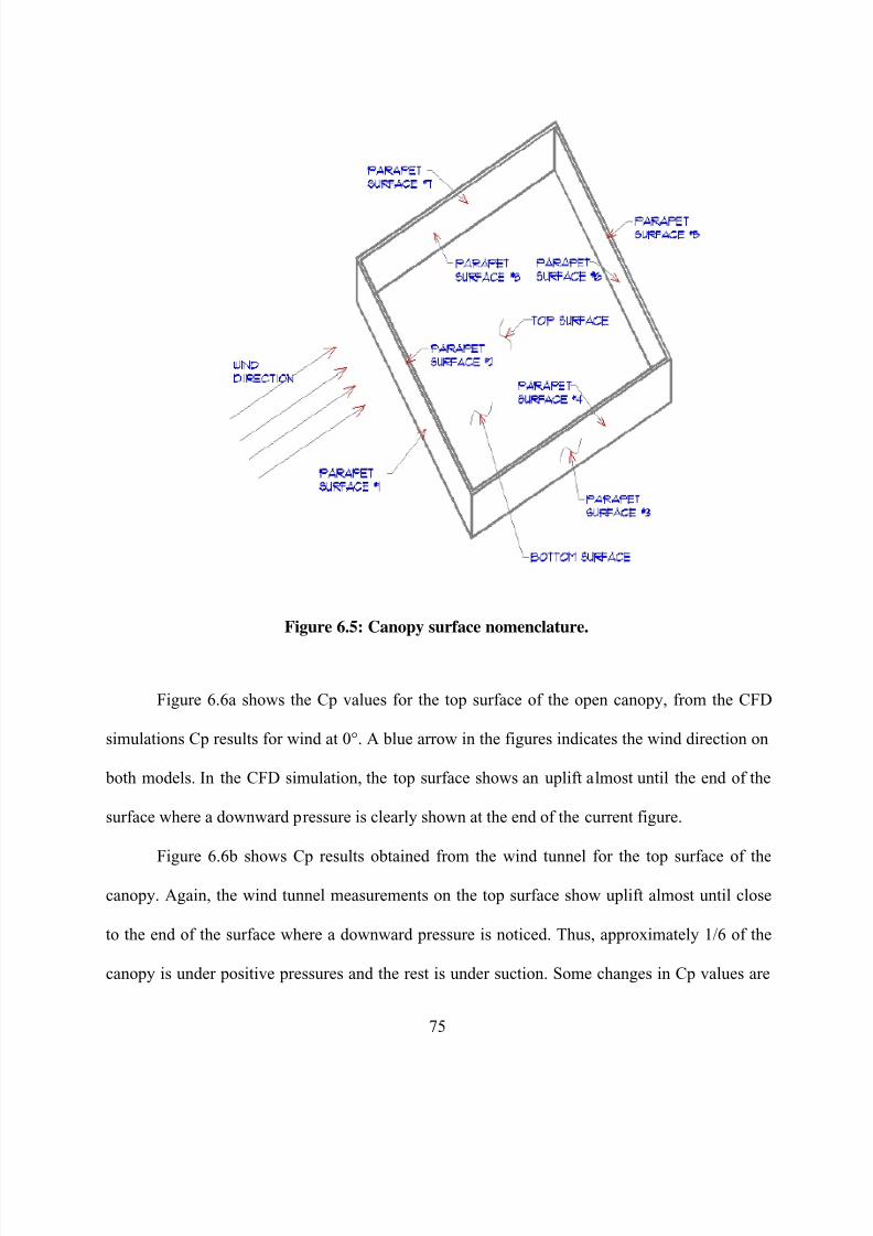
8/22/2019 Open Canopy Wind With Parapets
http://slidepdf.com/reader/full/open-canopy-wind-with-parapets 99/275
75
Figure 6.5: Canopy surface nomenclature.
Figure 6.6a shows the Cp values for the top surface of the open canopy, from the CFD
simulations Cp results for wind at 0°. A blue arrow in the figures indicates the wind direction on
both models. In the CFD simulation, the top surface shows an uplift almost until the end of the
surface where a downward pressure is clearly shown at the end of the current figure.
Figure 6.6b shows Cp results obtained from the wind tunnel for the top surface of the
canopy. Again, the wind tunnel measurements on the top surface show uplift almost until close
to the end of the surface where a downward pressure is noticed. Thus, approximately 1/6 of the
canopy is under positive pressures and the rest is under suction. Some changes in Cp values are
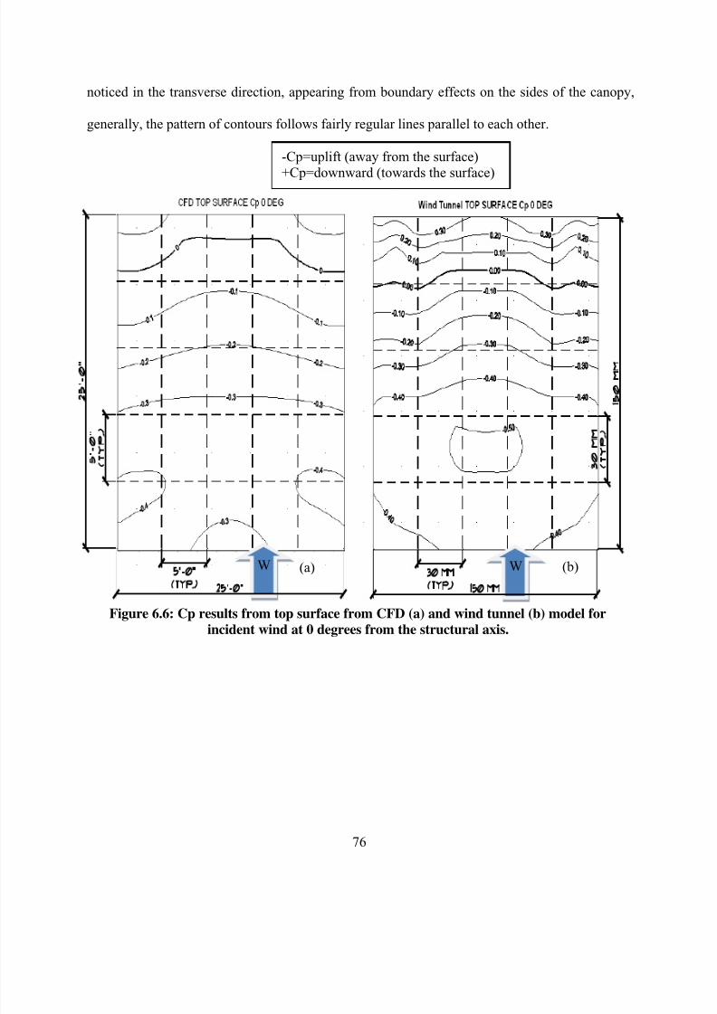
8/22/2019 Open Canopy Wind With Parapets
http://slidepdf.com/reader/full/open-canopy-wind-with-parapets 100/275
76
noticed in the transverse direction, appearing from boundary effects on the sides of the canopy,
generally, the pattern of contours follows fairly regular lines parallel to each other.
Figure 6.6: Cp results from top surface from CFD (a) and wind tunnel (b) model forincident wind at 0 degrees from the structural axis.
-Cp=uplift (away from the surface)
+Cp=downward (towards the surface)
W W(a) (b)

8/22/2019 Open Canopy Wind With Parapets
http://slidepdf.com/reader/full/open-canopy-wind-with-parapets 101/275
77
6.3 CFD and wind tunnel results for bottom surface, wind at 0
degrees
Figure 6.7: Cp results from bottom surface CFD (a) and wind tunnel (b) model for incident
wind at 0 degrees from the structural axis.
Figure 6.7a show the Cp values for the bottom surface of the canopy using CFD, for the
wind at 0°. The bottom surface shows on both, the wind tunnel and the CFD simulation, uniform
downward pressure through the entire bottom surface.
The Cp values for the bottom surface of the canopy at the wind tunnel for the wind at 0°
are shown in Figure 6.7b. The wind tunnel results have an almost uniform downward pressure
gradient affecting the entire bottom surface. The comparisons indicate that Cp values derived
W W(a) (b)
-Cp=uplift (away from the surface)
+Cp=downward (towards the surface)
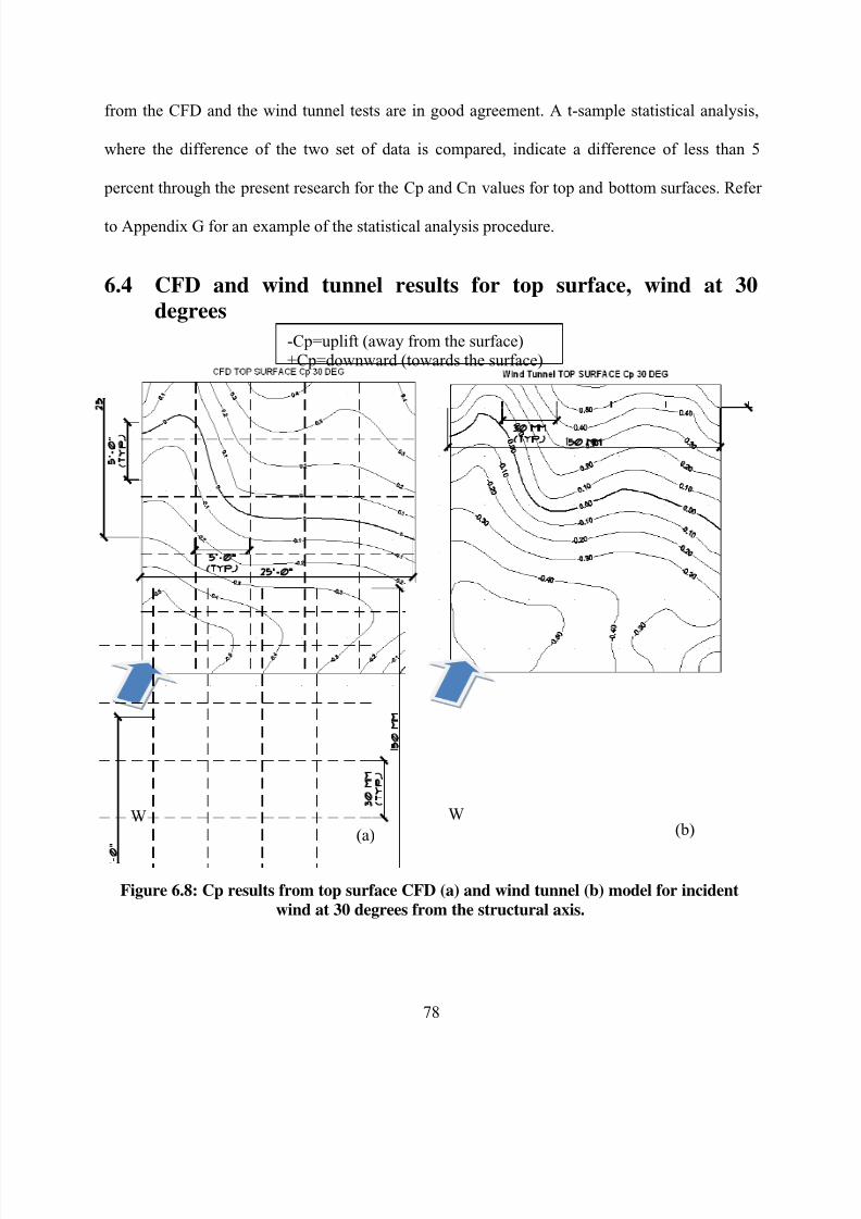
8/22/2019 Open Canopy Wind With Parapets
http://slidepdf.com/reader/full/open-canopy-wind-with-parapets 102/275
78
from the CFD and the wind tunnel tests are in good agreement. A t-sample statistical analysis,
where the difference of the two set of data is compared, indicate a difference of less than 5
percent through the present research for the Cp and Cn values for top and bottom surfaces. Refer
to Appendix G for an example of the statistical analysis procedure.
6.4 CFD and wind tunnel results for top surface, wind at 30
degrees
Figure 6.8: Cp results from top surface CFD (a) and wind tunnel (b) model for incident
wind at 30 degrees from the structural axis.
W W
(a) (b)
-Cp=uplift (away from the surface)+Cp=downward (towards the surface)

8/22/2019 Open Canopy Wind With Parapets
http://slidepdf.com/reader/full/open-canopy-wind-with-parapets 103/275
79
Figure 6.8a shows the Cp values for the top surface of the canopy, obtained with CFD,
for the wind at 30°. The CFD simulation on the top surface shows an uplift for the first half of
the top surface (windward region) and a downward pressure on the other half (leeward).
Next, a configuration at 30° was investigated by rotating the turntable in the wind tunnel.
Figure 6.8b shows the Cp values for the top surface of the canopy from the wind tunnel for the
wind at 30°, indicating that there is an uplift on the first half (windward region) of the top surface
and a downward pressure on the other half (leeward). This effect is clearly shown on both of the
previous figures (Figure 6.8a and 6.8b).
6.5 CFD and wind tunnel results for bottom surface, wind at 30
degrees
Figure 6.9a shows the CFD Cp values for the bottom surface of the canopy for the wind
at 30°. The bottom surface shows uniform negative Cp values, meaning that there is an uplift
pressure on the surface, i.e. downward pressure (suction) through the entire bottom surface.
Figure 6.9b shows the Cp values for the bottom surface of the canopy for the wind tunnel
for the wind at 30° incident angle. The bottom surface shows on the wind tunnel and uniform
downward pressure through the entire bottom surface. Both figures are in good agreement
regarding the values obtained.
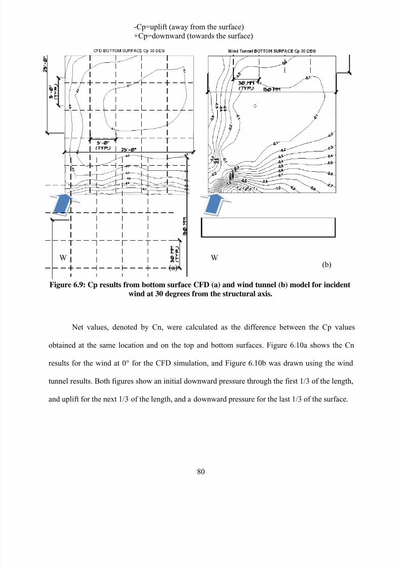
8/22/2019 Open Canopy Wind With Parapets
http://slidepdf.com/reader/full/open-canopy-wind-with-parapets 104/275
80
Figure 6.9: Cp results from bottom surface CFD (a) and wind tunnel (b) model for incident
wind at 30 degrees from the structural axis.
Net values, denoted by Cn, were calculated as the difference between the Cp values
obtained at the same location and on the top and bottom surfaces. Figure 6.10a shows the Cn
results for the wind at 0° for the CFD simulation, and Figure 6.10b was drawn using the wind
tunnel results. Both figures show an initial downward pressure through the first 1/3 of the length,
and uplift for the next 1/3 of the length, and a downward pressure for the last 1/3 of the surface.
W W
(a) (b)
-Cp=uplift (away from the surface)
+Cp=downward (towards the surface)

8/22/2019 Open Canopy Wind With Parapets
http://slidepdf.com/reader/full/open-canopy-wind-with-parapets 105/275
81
Figure 6.10: Cn results from CFD (a) and wind tunnel (b) model for incident wind at 0
degrees from the structural axis.
Cn results for the wind at 30° are shown on Figure 6.11a and Figure 6.11b. The net
pressures in this case show an uplift area located in the center of the surface, with a downward
pressure zone around that uplift center area. The wind in both studies, the CFD and the wind
tunnel, are in good agreement in the location of the areas where uplift and downward pressure
are located.
W W(a) (b)
-Cn=uplift (away from the surface)
+Cn=downward (towards the surface)
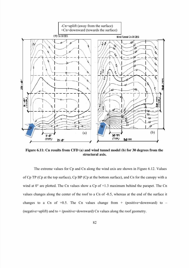
8/22/2019 Open Canopy Wind With Parapets
http://slidepdf.com/reader/full/open-canopy-wind-with-parapets 106/275
82
Figure 6.11: Cn results from CFD (a) and wind tunnel model (b) for 30 degrees from the
structural axis.
The extreme values for Cp and Cn along the wind axis are shown in Figure 6.12. Values
of Cp TP (Cp at the top surface), Cp BP (Cp at the bottom surface), and Cn for the canopy with a
wind at 0° are plotted. The Cn values show a Cp of +1.3 maximum behind the parapet. The Cn
values changes along the center of the roof to a Cn of -0.5, whereas at the end of the surface it
changes to a Cn of +0.5. The Cn values change from + (positive=downward) to –
(negative=uplift) and to + (positive=downward) Cn values along the roof geometry.
W W
(a) (b)
-Cn=uplift (away from the surface)+Cn=downward (towards the surface)

8/22/2019 Open Canopy Wind With Parapets
http://slidepdf.com/reader/full/open-canopy-wind-with-parapets 107/275
83
Figure 6.12: Cp and Cn results for CFD model at 0 degrees for (25x25x4 ft) canopy.
6.6 CFD and wind tunnel results for parapets, wind at 0 degrees
Cp values for the parapet surface #1 at 0° for CFD and wind tunnel are shown in Figure
6.13a and Figure 6.13b. Positive Cp values indicating pressure downward on the surface. Values
vary from +0.9 to +1.1.
-Cp or -Cn=uplift (away from the surface)
+Cp or +Cn=downward (towards the surface)

8/22/2019 Open Canopy Wind With Parapets
http://slidepdf.com/reader/full/open-canopy-wind-with-parapets 108/275
84
Figure 6.13: Cp results at parapet surface #1 at 0 degrees from CFD (a) and wind tunnel(b).
Cp values for the parapet surface #2 at 0° for CFD and wind tunnel are shown in Figure
6.14a and Figure 6.14b. Negative Cp values indicating uplift pressure away from the surface.
Values vary from -0.3 to -0.4.
(a)
(b)
w
-Cp=uplift (away from the surface)+Cp=downward (towards the surface)

8/22/2019 Open Canopy Wind With Parapets
http://slidepdf.com/reader/full/open-canopy-wind-with-parapets 109/275
85
Figure 6.14: Cp results at parapet surface #2 at 0 degrees for CFD (a) and wind tunnel (b).
Cp values for the parapet surface #3 and parapet surface #7 at 0° for CFD and wind
tunnel are shown in Figure 6.15a and Figure 6.15b. Negative Cp values indicating uplift pressure
away from the surface. Values vary from -0.9 to -0.1.
(a)
(b)
w
-Cp=uplift (away from the surface)+Cp=downward (towards the surface)
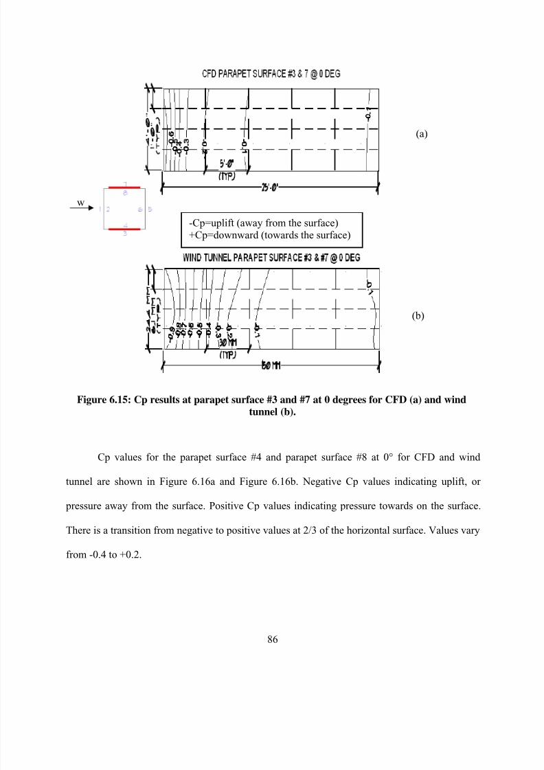
8/22/2019 Open Canopy Wind With Parapets
http://slidepdf.com/reader/full/open-canopy-wind-with-parapets 110/275
86
Figure 6.15: Cp results at parapet surface #3 and #7 at 0 degrees for CFD (a) and windtunnel (b).
Cp values for the parapet surface #4 and parapet surface #8 at 0° for CFD and wind
tunnel are shown in Figure 6.16a and Figure 6.16b. Negative Cp values indicating uplift, or
pressure away from the surface. Positive Cp values indicating pressure towards on the surface.
There is a transition from negative to positive values at 2/3 of the horizontal surface. Values vary
from -0.4 to +0.2.
(a)
(b)
w
-Cp=uplift (away from the surface)+Cp=downward (towards the surface)
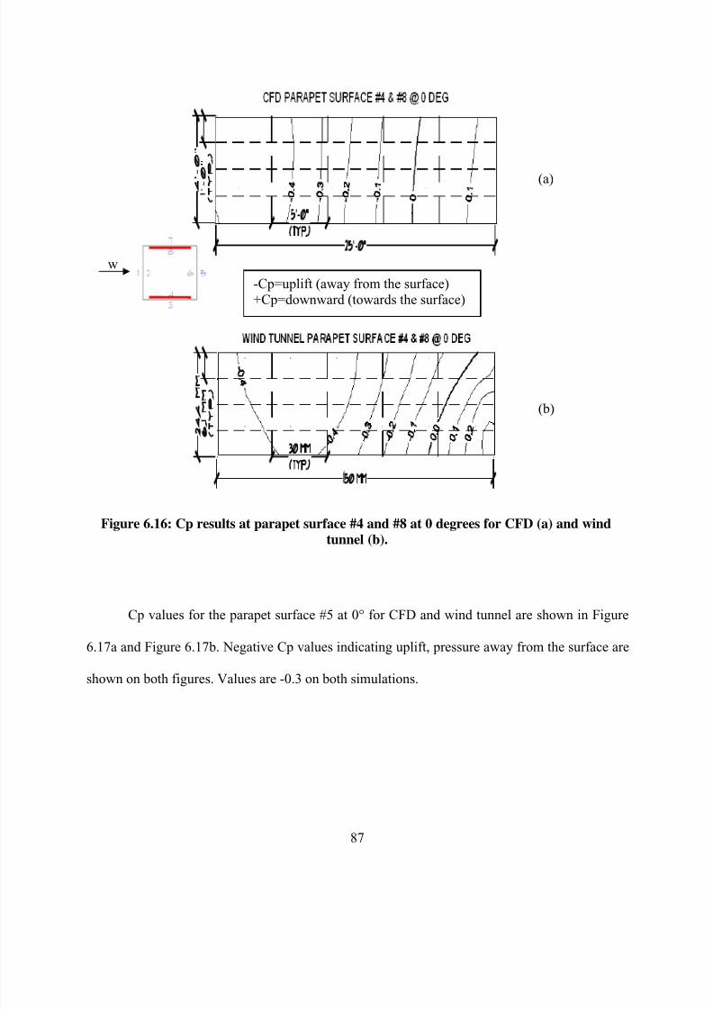
8/22/2019 Open Canopy Wind With Parapets
http://slidepdf.com/reader/full/open-canopy-wind-with-parapets 111/275
87
Figure 6.16: Cp results at parapet surface #4 and #8 at 0 degrees for CFD (a) and windtunnel (b).
Cp values for the parapet surface #5 at 0° for CFD and wind tunnel are shown in Figure
6.17a and Figure 6.17b. Negative Cp values indicating uplift, pressure away from the surface are
shown on both figures. Values are -0.3 on both simulations.
(a)
(b)
w
-Cp=uplift (away from the surface)+Cp=downward (towards the surface)

8/22/2019 Open Canopy Wind With Parapets
http://slidepdf.com/reader/full/open-canopy-wind-with-parapets 112/275
88
Figure 6.17: Cp results at parapet surface #5 at 0 degrees for CFD (a) and wind tunnel (b).
Cp values for the parapet surface #6 at 0° for CFD and wind tunnel are shown in Figure
6.18a and Figure 6.18b. Positive Cp values indicating pressure downward on the surface are
shown on both figures. Values vary from +0.1 to +0.2.
(a)
(b)
w
-Cp=uplift (away from the surface)+Cp=downward (towards the surface)

8/22/2019 Open Canopy Wind With Parapets
http://slidepdf.com/reader/full/open-canopy-wind-with-parapets 113/275
89
Figure 6.18: Cp results at parapet surface #6 at 0 degrees for CFD (a) and wind tunnel (b).
Cn values for the parapet surface #1 and parapet surface #2 at 0° for CFD and wind
tunnel are shown in Figure 6.19a and Figure 6.19b. Net positive values indicating pressure
downward on the surface is shown on both figures. Values vary from +1.2 to +1.5.
(a)
(b)
w
-Cp=uplift (away from the surface)+Cp=downward (towards the surface)

8/22/2019 Open Canopy Wind With Parapets
http://slidepdf.com/reader/full/open-canopy-wind-with-parapets 114/275
90
Figure 6.19: Cn results at parapet surface #1 and 2 at 0 degrees for CFD (a) and wind
tunnel (b).
Cn values for the parapet surface #3 and parapet surface #4 at 0° for CFD and wind tunnel are
shown in Figure 6.20a and Figure 6.20b. Net negative and positive values indicating changes in
pressure downward and uplift on the surface is shown in both figures. Values vary from -0.5 to
be 0.0 the first 1/3 of the horizontal surface. Cn values for the parapet surface #3 and parapet
surface #4 at 0° for CFD and wind tunnel are shown in Figure 6.20a and Figure 6.20b.
(a)
(b)
w
-Cn=uplift (away from the surface)+Cn=downward (towards the surface)

8/22/2019 Open Canopy Wind With Parapets
http://slidepdf.com/reader/full/open-canopy-wind-with-parapets 115/275
91
Figure 6.20: Cn results at parapet surface #3 and 4 at 0 degrees for CFD (a) and windtunnel (b).
Net negative and positive values indicating changes in pressure downward and uplift on
the surface is shown in both figures. Values vary from -0.5 to be 0.0 the first 1/3 of the horizontal
surface. The values continue changing from 0.0 to +0.3 and to 0.0 for 2/3 of the horizontal
surface. The last 1/3 of the horizontal surface, Cn surface values changes from 0.0 to -0.3. The
CFD simulation is able to capture the transition between the changes in downward pressure and
uplift. The values at the beginning of the horizontal surface are higher on the wind tunnel parapet
surface.
(a)
(b)
w
-Cn=uplift (away from the surface)+Cn=downward (towards the surface)

8/22/2019 Open Canopy Wind With Parapets
http://slidepdf.com/reader/full/open-canopy-wind-with-parapets 116/275
92
Cn values for the parapet surface #5 and parapet surface #6 at 0° for CFD and wind
tunnel are shown on Figure 6.21a and Figure 6.21b. Net negative values indicating uplift on the
surface is shown on both figures. Values vary from -0.5 to -0.4.
Figure 6.21: Cn results at parapet surface #5 and 6 at 0 degrees for CFD (a) and wind
tunnel (b).
Cn values for the parapet surface #7 and parapet surface #8 at 0° for CFD and wind
tunnel are shown on Figure 6.22a and Figure 6.22b. Net negative and positive values indicating
changes in pressure towards and away on the surface are shown on both figures.
(a)
(b)
w
-Cn=uplift (away from the surface)+Cn=downward (towards the surface)
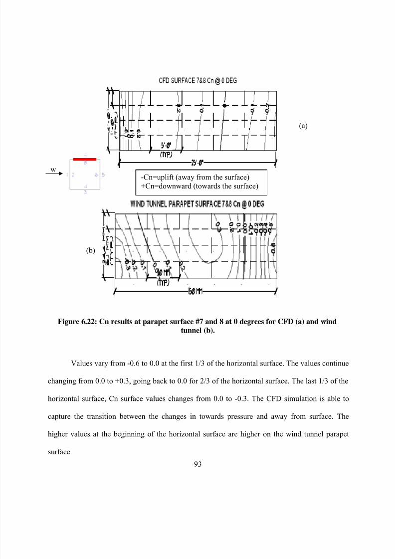
8/22/2019 Open Canopy Wind With Parapets
http://slidepdf.com/reader/full/open-canopy-wind-with-parapets 117/275
93
Figure 6.22: Cn results at parapet surface #7 and 8 at 0 degrees for CFD (a) and windtunnel (b).
Values vary from -0.6 to 0.0 at the first 1/3 of the horizontal surface. The values continue
changing from 0.0 to +0.3, going back to 0.0 for 2/3 of the horizontal surface. The last 1/3 of the
horizontal surface, Cn surface values changes from 0.0 to -0.3. The CFD simulation is able to
capture the transition between the changes in towards pressure and away from surface. The
higher values at the beginning of the horizontal surface are higher on the wind tunnel parapet
surface.
(a)
(b)
w-Cn=uplift (away from the surface)
+Cn=downward (towards the surface)
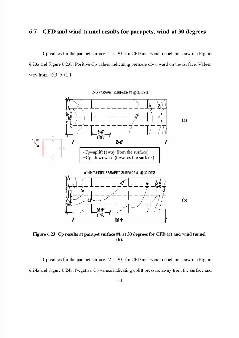
8/22/2019 Open Canopy Wind With Parapets
http://slidepdf.com/reader/full/open-canopy-wind-with-parapets 118/275
94
6.7 CFD and wind tunnel results for parapets, wind at 30 degrees
Cp values for the parapet surface #1 at 30° for CFD and wind tunnel are shown in Figure
6.23a and Figure 6.23b. Positive Cp values indicating pressure downward on the surface. Values
vary from +0.5 to +1.1.
Figure 6.23: Cp results at parapet surface #1 at 30 degrees for CFD (a) and wind tunnel
(b).
Cp values for the parapet surface #2 at 30° for CFD and wind tunnel are shown in Figure
6.24a and Figure 6.24b. Negative Cp values indicating uplift pressure away from the surface and
(a)
(b)
w
-Cp=uplift (away from the surface)
+Cp=downward (towards the surface)

8/22/2019 Open Canopy Wind With Parapets
http://slidepdf.com/reader/full/open-canopy-wind-with-parapets 119/275
95
a transition zone where the Cp values changes from negative to positive values at the last 1/6 of
the horizontal surface. Values vary from -0.5 to +0.1.
Figure 6.24: Cp results at parapet surface #2 at 30 degrees for CFD (a) and wind tunnel
(b).
Cp values for the parapet surface #3 and parapet surface #7 at 30° for CFD and wind
tunnel are shown in Figure 6.25a and Figure 6.25b. Negative Cp values indicating uplift pressure
away from the surface. Values vary from -0.7 to -0.2.
(a)
(b)
w
-Cp=uplift (away from the surface)
+Cp=downward (towards the surface)

8/22/2019 Open Canopy Wind With Parapets
http://slidepdf.com/reader/full/open-canopy-wind-with-parapets 120/275
96
Figure 6.25: Cp results at parapet surface #3 at 30 degrees for CFD (a) and wind tunnel(b).
Cp values for the parapet surface #4 at 30° for CFD and wind tunnel are shown in Figure
6.26a and Figure 6.26b. Negative Cp values indicating uplift, pressure away from the surface.
Positive Cp values indicating pressure downward on the surface. There is a transition from
negative to positive values at 1/2 of the horizontal surface. Values vary from -0.2 to 0.0 on the
first half, and from 0.0 to 0.7 on the second half.
(a)
(b)
w
-Cp=uplift (away from the surface)
+Cp=downward (towards the surface)
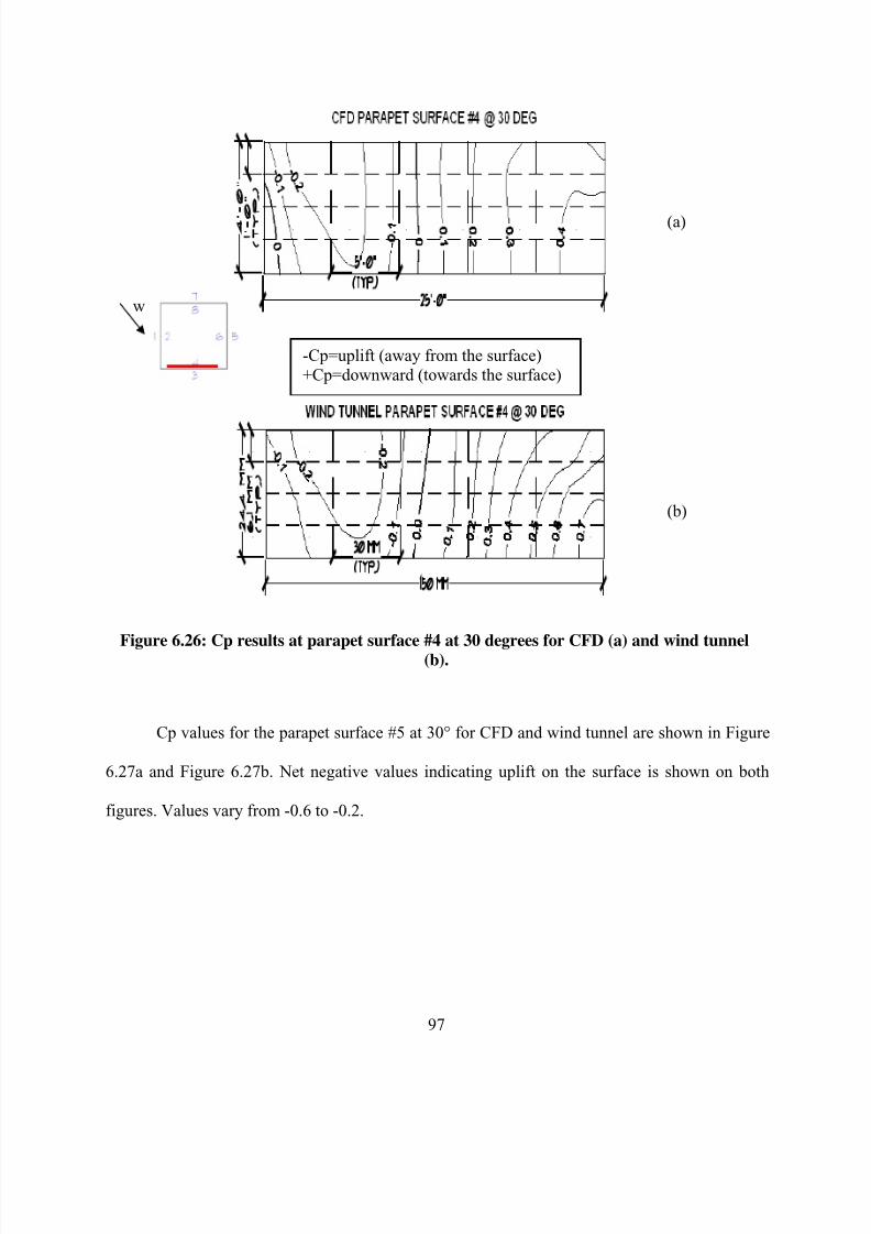
8/22/2019 Open Canopy Wind With Parapets
http://slidepdf.com/reader/full/open-canopy-wind-with-parapets 121/275
97
Figure 6.26: Cp results at parapet surface #4 at 30 degrees for CFD (a) and wind tunnel(b).
Cp values for the parapet surface #5 at 30° for CFD and wind tunnel are shown in Figure
6.27a and Figure 6.27b. Net negative values indicating uplift on the surface is shown on both
figures. Values vary from -0.6 to -0.2.
(a)
(b)
w
-Cp=uplift (away from the surface)+Cp=downward (towards the surface)

8/22/2019 Open Canopy Wind With Parapets
http://slidepdf.com/reader/full/open-canopy-wind-with-parapets 122/275
98
Figure 6.27: Cp results at parapet surface #5 at 30 degrees for CFD (a) and wind tunnel(b).
Cp values for the parapet surface #6 at 30° for CFD and wind tunnel are shown in Figure
6.28a and Figure 6.28b. Positive net values indicating downward pressure on the surface is
shown on both figures. There is a small region where the values changes from positive to
negative Cp values at the end of the horizontal surface. Values vary from +0.6 to 0.0.
(a)
(b)
w
-Cp=uplift (away from the surface)
+Cp=downward (towards the surface)

8/22/2019 Open Canopy Wind With Parapets
http://slidepdf.com/reader/full/open-canopy-wind-with-parapets 123/275
99
Figure 6.28: Cp results at parapet surface #6 at 30 degrees for CFD (a) and wind tunnel
(b).
Cp values for the parapet surface #7 at 30° for CFD and wind tunnel are shown in Figure
6.29a and Figure 6.29b. Positive Cp values indicating towards pressure on the surface are shown
on both figures. Values vary from +0.4 to +0.1.
(a)
(b)
w
-Cp=uplift (away from the surface)+Cp=downward (towards the surface)

8/22/2019 Open Canopy Wind With Parapets
http://slidepdf.com/reader/full/open-canopy-wind-with-parapets 124/275
100
Figure 6.29: Cp results at parapet surface #7 at 30 degrees for CFD (a) and wind tunnel
(b).
Cp values for the parapet surface #8 at 30° for CFD and wind tunnel are shown in Figure
6.30a and Figure 6.30b. Negative Cp values indicating uplift, pressure away from the surface.
Positive Cp values indicating pressure downward on the surface. There is a transition from
negative to positive values at 2/3 of the horizontal surface. Values vary from -0.4 to 0.0 and from
0.0 to +0.3.
(a)
(b)
w
-Cp=uplift (away from the surface)
+Cp=downward (towards the surface)

8/22/2019 Open Canopy Wind With Parapets
http://slidepdf.com/reader/full/open-canopy-wind-with-parapets 125/275
101
Figure 6.30: Cp results at parapet surface #8 at 30 degrees for CFD (a) and wind tunnel
(b).
Cn values for the parapet surface #1 and parapet surface #2 at 30° for CFD and wind
tunnel are shown in Figure 6.31a and Figure 6.31b. Net positive values indicating pressure
downward on the surface is shown on both figures. Values vary from +1.5 to +0.5.
(a)
(b)
w
-Cp=uplift (away from the surface)
+Cp=downward (towards the surface)

8/22/2019 Open Canopy Wind With Parapets
http://slidepdf.com/reader/full/open-canopy-wind-with-parapets 126/275
102
Figure 6.31: Cn results at parapet surface #1 and 2 at 30 degrees for CFD (a) and wind
tunnel (b).
Cn values for the parapet surface #3 and parapet surface #4 at 30° for CFD and wind
tunnel are shown in Figure 6.32a and Figure 6.32b. Net negative values indicating changes in
pressure and uplift on the surface are shown on both figures. Values vary from -0.9 to -0.3 for
the first 1/2 of the horizontal surface. The values continue changing from -0.3 to -0.6 at the end
of the horizontal surface.
(a)
(b)
w
-Cn=uplift (away from the surface)
+Cn=downward (towards the surface)
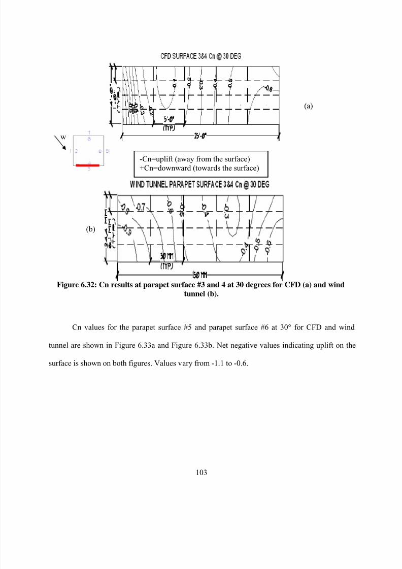
8/22/2019 Open Canopy Wind With Parapets
http://slidepdf.com/reader/full/open-canopy-wind-with-parapets 127/275
103
Figure 6.32: Cn results at parapet surface #3 and 4 at 30 degrees for CFD (a) and wind
tunnel (b).
Cn values for the parapet surface #5 and parapet surface #6 at 30° for CFD and wind
tunnel are shown in Figure 6.33a and Figure 6.33b. Net negative values indicating uplift on the
surface is shown on both figures. Values vary from -1.1 to -0.6.
(a)
(b)
w
-Cn=uplift (away from the surface)
+Cn=downward (towards the surface)

8/22/2019 Open Canopy Wind With Parapets
http://slidepdf.com/reader/full/open-canopy-wind-with-parapets 128/275
104
Figure 6.33: Cn results at parapet surface #5 and 6 at 30 degrees for CFD (a) and windtunnel (b).
Cn values for the parapet surface #7 and parapet surface #8 at 30° for CFD and wind
tunnel are shown in Figure 6.34a and Figure 6.34b. Net positive and negative values indicating
changes in uplift and pressure downward are shown on both figures. Values vary from +0.9 to
0.0 until the last 1/6 of the horizontal surface. The values continue changing from 0.0 to -0.3 on
the last 1/6 of the horizontal surface.
(a)
(b)
w
-Cn=uplift (away from the surface)
+Cn=downward (towards the surface)
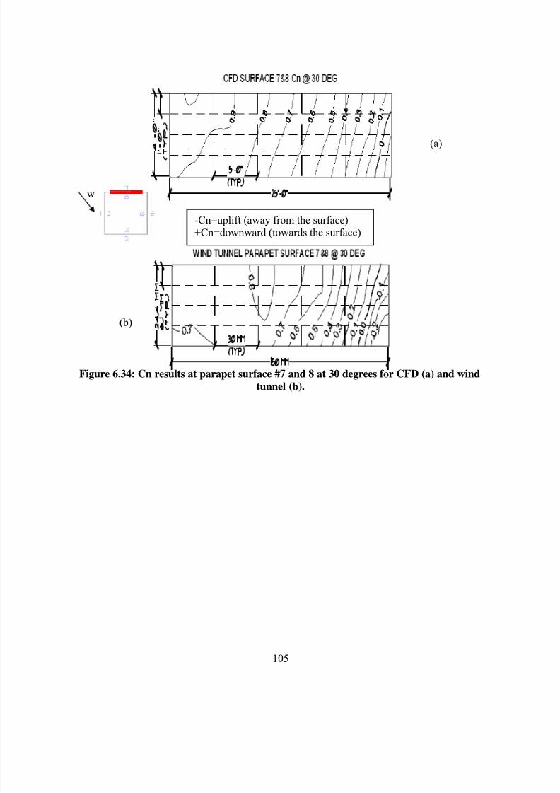
8/22/2019 Open Canopy Wind With Parapets
http://slidepdf.com/reader/full/open-canopy-wind-with-parapets 129/275
105
Figure 6.34: Cn results at parapet surface #7 and 8 at 30 degrees for CFD (a) and wind
tunnel (b).
(a)
(b)
w
-Cn=uplift (away from the surface)+Cn=downward (towards the surface)

8/22/2019 Open Canopy Wind With Parapets
http://slidepdf.com/reader/full/open-canopy-wind-with-parapets 130/275
106
CHAPTER 7. PARAMETRIC STUDIES OF PRESSURE
COEFFICIENTS IN CANOPIES USING CFD
7.1 Description
The results of the previous chapter shows that EFD.Lab, the CFD computer program used
in this investigation, can generate similar Cp values in comparison to the wind tunnel results. For
the CFD computations and the wind tunnel tests, only one configuration has been tested, the
canopy with dimensions 7.6 m (25ft) x 7.6 m (25 ft) and parapet of 1.22 m (4 ft). However, it is
necessary to investigate different geometries in order to determine how the Cp and the Cn values
vary with the plan geometry and parapet differences, and establish design Cn values based on
those results.
Three different configurations are investigated in this chapter. Each configuration is
investigated individually with four different parapet heights. Figure 7.1 indicates the
nomenclature used for the canopy geometry. Four different parapet heights are investigated in
combination with the different plan models. Parapet heights attempt to represent realistic cases
and vary from 0.91 m (3 ft), 1.22 m (4 ft), 1.52 m (5 ft) and 1.83 m (6 ft). Two different wind
directions are modeled using the CFD program, 0 and 30 degrees as done on the wind tunnel.
The combination of all the plan and parapet geometries generates a total of 24 models to be
investigated.
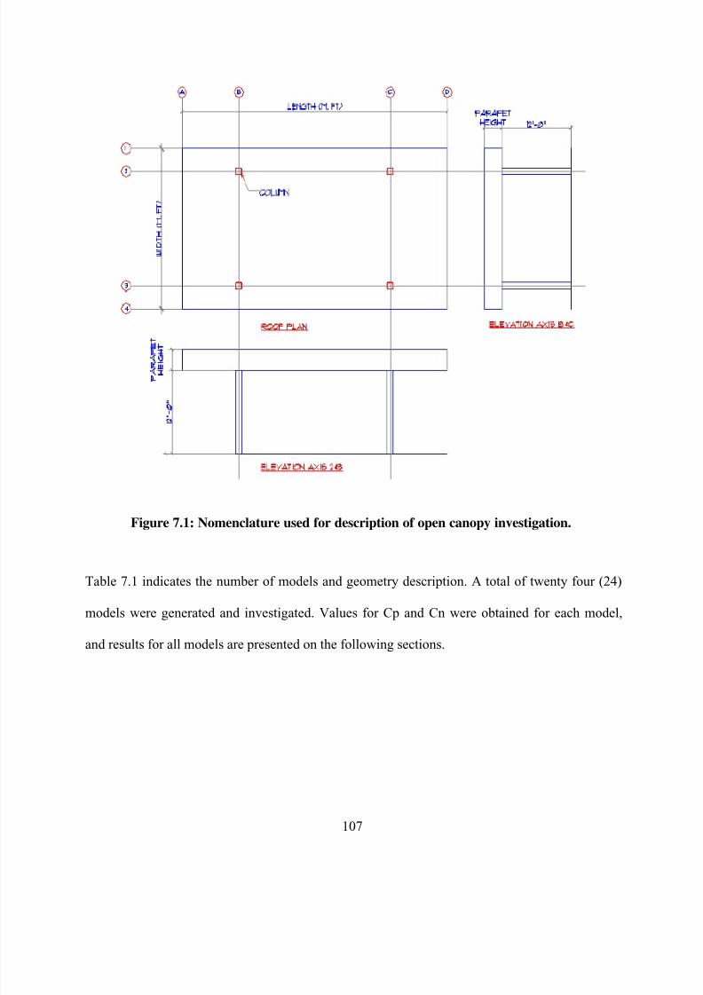
8/22/2019 Open Canopy Wind With Parapets
http://slidepdf.com/reader/full/open-canopy-wind-with-parapets 131/275
107
Figure 7.1: Nomenclature used for description of open canopy investigation.
Table 7.1 indicates the number of models and geometry description. A total of twenty four (24)
models were generated and investigated. Values for Cp and Cn were obtained for each model,
and results for all models are presented on the following sections.

8/22/2019 Open Canopy Wind With Parapets
http://slidepdf.com/reader/full/open-canopy-wind-with-parapets 132/275
108
Table 7.1: Model geometry description for the CFD parametric study.
Model #
ModelDescription(LxWxPH)
Width Length Parapet heightWind
Angle
m ft m ft m ft degrees
1 25x25x3 0 DEG 7.62 25 7.62 25 0.91 3 0
2 25x25x3 30 DEG 7.62 25 7.62 25 0.91 3 30
3 25x25x4 0 DEG 7.62 25 7.62 25 1.22 4 0
4 25x25x4 30 DEG 7.62 25 7.62 25 1.22 4 30
5 25x25x5 0 DEG 7.62 25 7.62 25 1.52 5 0
6 25x25x5 30 DEG 7.62 25 7.62 25 1.52 5 30
7 25x25x6 0 DEG 7.62 25 7.62 25 1.83 6 0
8 25x25x6 30 DEG 7.62 25 7.62 25 1.83 6 30
9 25x40x3 0 DEG 7.62 25 12.19 40 0.91 3 0
10 25x40x3 30 DEG 7.62 25 12.19 40 0.91 3 30
11 25x40x4 0 DEG 7.62 25 12.19 40 1.22 4 0
12 25x40x4 30 DEG 7.62 25 12.19 40 1.22 4 30
13 25x40x5 0 DEG 7.62 25 12.19 40 1.52 5 0
14 25x40x5 30 DEG 7.62 25 12.19 40 1.52 5 30
15 25x40x6 0 DEG 7.62 25 12.19 40 1.83 6 0
16 25x40x6 30 DEG 7.62 25 12.19 40 1.83 6 30
17 25x50x3 0 DEG 7.62 25 15.24 50 0.91 3 0
18 25x50x3 30 DEG 7.62 25 15.24 50 0.91 3 30
19 25x50x4 0 DEG 7.62 25 15.24 50 1.22 4 0
20 25x50x4 30 DEG 7.62 25 15.24 50 1.22 4 30
21 25x50x5 0 DEG 7.62 25 15.24 50 1.52 5 0
22 25x50x5 30 DEG 7.62 25 15.24 50 1.52 5 30
23 25x50x6 0 DEG 7.62 25 15.24 50 1.83 6 0
24 25x50x6 30 DEG 7.62 25 15.24 50 1.83 6 30
CFD model results are represented in two different graphical formats. First, top view of
the contour surface representing the Cn values is presented for each model. Second, a 3D contour
plot showing the Cn values are also represented. The purpose of that graphical representation is
that it helps the visualization of the Cn values. The maximum and minimum are clearly
represented, especially when the wind is applied at 30 degrees from the structural axis to the
model.
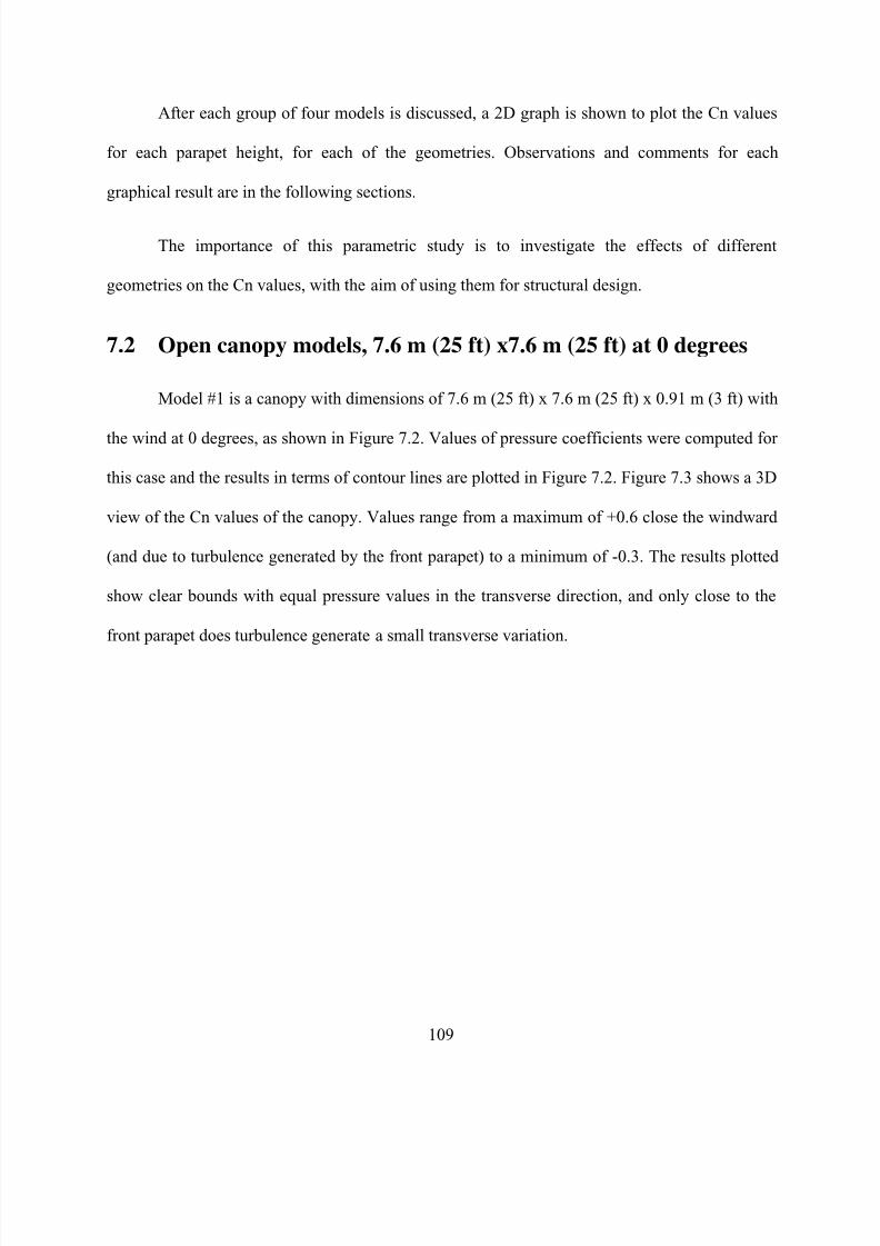
8/22/2019 Open Canopy Wind With Parapets
http://slidepdf.com/reader/full/open-canopy-wind-with-parapets 133/275
109
After each group of four models is discussed, a 2D graph is shown to plot the Cn values
for each parapet height, for each of the geometries. Observations and comments for each
graphical result are in the following sections.
The importance of this parametric study is to investigate the effects of different
geometries on the Cn values, with the aim of using them for structural design.
7.2 Open canopy models, 7.6 m (25 ft) x7.6 m (25 ft) at 0 degrees
Model #1 is a canopy with dimensions of 7.6 m (25 ft) x 7.6 m (25 ft) x 0.91 m (3 ft) with
the wind at 0 degrees, as shown in Figure 7.2. Values of pressure coefficients were computed for
this case and the results in terms of contour lines are plotted in Figure 7.2. Figure 7.3 shows a 3D
view of the Cn values of the canopy. Values range from a maximum of +0.6 close the windward
(and due to turbulence generated by the front parapet) to a minimum of -0.3. The results plotted
show clear bounds with equal pressure values in the transverse direction, and only close to the
front parapet does turbulence generate a small transverse variation.

8/22/2019 Open Canopy Wind With Parapets
http://slidepdf.com/reader/full/open-canopy-wind-with-parapets 134/275
110
Figure 7.2: Model #1, contour plan for Cn values for wind at 0 degrees.
Figure 7.3: Model #1, 3D contour plot for Cn values for wind at 0 degrees.
W
W

8/22/2019 Open Canopy Wind With Parapets
http://slidepdf.com/reader/full/open-canopy-wind-with-parapets 135/275
111
For the same dimensions in plan, the new model has a higher parapet. Cn values for
contour plan for Model #3, with dimensions of 7.6 m (25 ft) x 7.6 m (25 ft) x 1.22 m (4 ft) with
the wind at 0 degrees are shown in Figure 7.4. Figure 7.5 shows a 3D view of the Cn values of
the canopy. Values range from a maximum of +0.8 to a minimum of -0.3. In comparison with the
previous model with a shorter parapet, the maximum positive values have increased from 0.6 to
0.8 for a change of parapet from 3 to 4 ft.
Figure 7.4: Model #3, contour plan for Cn values for wind at 0 degrees.
W

8/22/2019 Open Canopy Wind With Parapets
http://slidepdf.com/reader/full/open-canopy-wind-with-parapets 136/275
112
Figure 7.5: Model #3, 3D contour plot for Cn values for wind at 0 degrees.
A higher parapet is investigated in the next configuration. Cn values for contour plan for
Model #5, with dimensions of 7.6 m (25 ft) x 7.6 m (25 ft) x 1.52 m (5 ft) with the wind at 0
degrees are shown on Figure 7.6. Figure 7.7 shows a 3D view of the Cn values of the canopy.
Values range from a maximum of +0.9 to a minimum of -0.3.
W

8/22/2019 Open Canopy Wind With Parapets
http://slidepdf.com/reader/full/open-canopy-wind-with-parapets 137/275
113
Figure 7.6: Model #5, contour plan for Cn values for wind at 0 degrees.
Figure 7.7: Model #5, 3D contour plot for Cn values for wind at 0 degrees.
W
W

8/22/2019 Open Canopy Wind With Parapets
http://slidepdf.com/reader/full/open-canopy-wind-with-parapets 138/275
114
Finally, the parapet is increased with respect to the previous models. Cn values for
contour plan for Model #7, with dimensions of 7.6 m (25 ft) x 7.6 m (25 ft) x 1.82 m (6 ft) with
the wind at 0 degrees, are shown on Figure 7.8. Figure 7.9 shows a 3D view of the Cn values of
the canopy. Values ranges from a maximum of +0.9 to a minimum of -0.3.
Figure 7.8: Model #7, contour plan for Cn values for wind at 0 degrees.
W
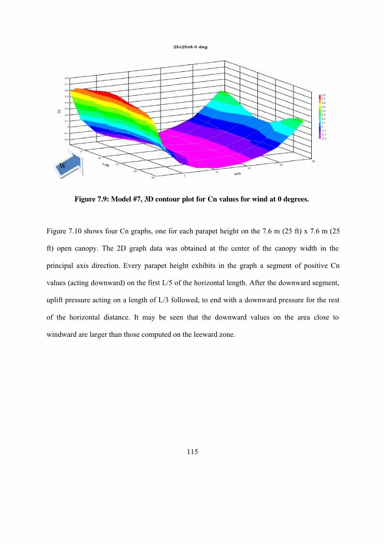
8/22/2019 Open Canopy Wind With Parapets
http://slidepdf.com/reader/full/open-canopy-wind-with-parapets 139/275
115
Figure 7.9: Model #7, 3D contour plot for Cn values for wind at 0 degrees.
Figure 7.10 shows four Cn graphs, one for each parapet height on the 7.6 m (25 ft) x 7.6 m (25
ft) open canopy. The 2D graph data was obtained at the center of the canopy width in the
principal axis direction. Every parapet height exhibits in the graph a segment of positive Cn
values (acting downward) on the first L/5 of the horizontal length. After the downward segment,
uplift pressure acting on a length of L/3 followed, to end with a downward pressure for the rest
of the horizontal distance. It may be seen that the downward values on the area close to
windward are larger than those computed on the leeward zone.
W

8/22/2019 Open Canopy Wind With Parapets
http://slidepdf.com/reader/full/open-canopy-wind-with-parapets 140/275
116
Figure 7.10: Influence of parapet height. 2D graph of Cn values for all 7.6 m (25 ft) x 7.6 m
(25 ft) @ 0 degrees.
7.3 Open canopy models, 7.6 m (25 ft) x7.6 m (25 ft) at 30 degrees
The configuration in the previous section was aligned with the wind direction; however,
other wind directions may lead to more stringent pressure values. Cn values for contour plan for
Model #2, with dimensions of 7.6 m (25 ft) x 7.6 m (25 ft) x 0.91 m (3 ft) with the wind at 30
degrees are shown in Figure 7.11. Figure 7.12 shows a 3D view of the Cn values of the canopy.
The results indicate an asymmetric pressure pattern in the canopy, in which two parapets seen to
play a role. Values range from a maximum of +0.8 to a minimum of -0.6. These values are
significantly higher than those computed for Model #1, which were +0.6 and -0.3 respectively.
-Cn=uplift (away from the surface)
+Cn=downward (towards the surface)

8/22/2019 Open Canopy Wind With Parapets
http://slidepdf.com/reader/full/open-canopy-wind-with-parapets 141/275
117
Figure 7.11: Model #2, contour plan for Cn values for wind at 30 degrees.
Figure 7.12: Model #2, 3D contour plot for Cn values for wind at 30 degrees.
W
W
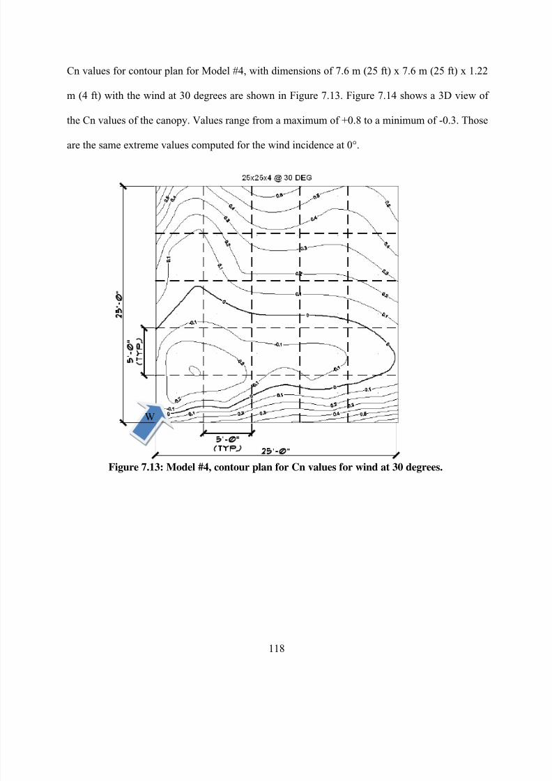
8/22/2019 Open Canopy Wind With Parapets
http://slidepdf.com/reader/full/open-canopy-wind-with-parapets 142/275
118
Cn values for contour plan for Model #4, with dimensions of 7.6 m (25 ft) x 7.6 m (25 ft) x 1.22
m (4 ft) with the wind at 30 degrees are shown in Figure 7.13. Figure 7.14 shows a 3D view of
the Cn values of the canopy. Values range from a maximum of +0.8 to a minimum of -0.3. Those
are the same extreme values computed for the wind incidence at 0°.
Figure 7.13: Model #4, contour plan for Cn values for wind at 30 degrees.
W

8/22/2019 Open Canopy Wind With Parapets
http://slidepdf.com/reader/full/open-canopy-wind-with-parapets 143/275
119
Figure 7.14: Model #4, 3D contour plot for Cn values for wind at 30 degrees.
Cn values for contour plan for Model #6, with dimensions of 7.6 m (25 ft) x 7.6 m (25 ft) x 1.52
m (5 ft) with the wind at 30 degrees are shown in Figure 7.15. Figure 7.16 shows a 3D view of
the Cn values of the canopy. Values range from a maximum of +0.9 to a minimum of -0.2, which
are similar to the values computed for Model #5 (with 0°).
W

8/22/2019 Open Canopy Wind With Parapets
http://slidepdf.com/reader/full/open-canopy-wind-with-parapets 144/275
120
Figure 7.15: Model #6, contour plan for Cn values for wind at 30 degrees.
Figure 7.16: Model #6, 3D contour plot for Cn values for wind at 30 degrees.
W
W

8/22/2019 Open Canopy Wind With Parapets
http://slidepdf.com/reader/full/open-canopy-wind-with-parapets 145/275
121
Cn values for contour plan for Model #8, with dimensions of 7.6 m (25 ft) x 7.6 m (25 ft) x 1.82
m (6 ft) with the wind at 30 degrees are shown in Figure 7.17. Figure 7.18 shows a 3D view of
the Cn values of the canopy. Values range from a maximum of +0.9 to a minimum of -0.2, which
are smaller than those computed at 0° (+1.0 and -0.2 respectively).
Figure 7.17: Model #8, contour plan for Cn values for wind at 30 degrees.
W

8/22/2019 Open Canopy Wind With Parapets
http://slidepdf.com/reader/full/open-canopy-wind-with-parapets 146/275
122
Figure 7.18: Model #8, 3D contour plot for Cn values for wind at 30 degrees.
Figure 7.19 shows four Cn graphs, one for each parapet height on the 7.6 m (25 ft) x 7.6 m (25
ft) open canopy. The 2D graph data was obtained at the center of the canopy width in the angle
of the applied wind, in these case thirty (30) degrees from the principal axis direction. All
parapet height exhibit on the graph a segment of positive Cn values (downward) on the first L/5,
except for the parapet height of 0.91 m (3 ft) and 1.22 m (4 ft), which were all negative Cn
values. After the uplift segment, an uplift pressure length of L/3 followed a downward for the
rest of the horizontal distance. As said before, the extreme values shown by 0° and 30° are
similar, but the actual distributions are the same, as can be seen from comparisons of Figures
7.10 and 7.19.
W
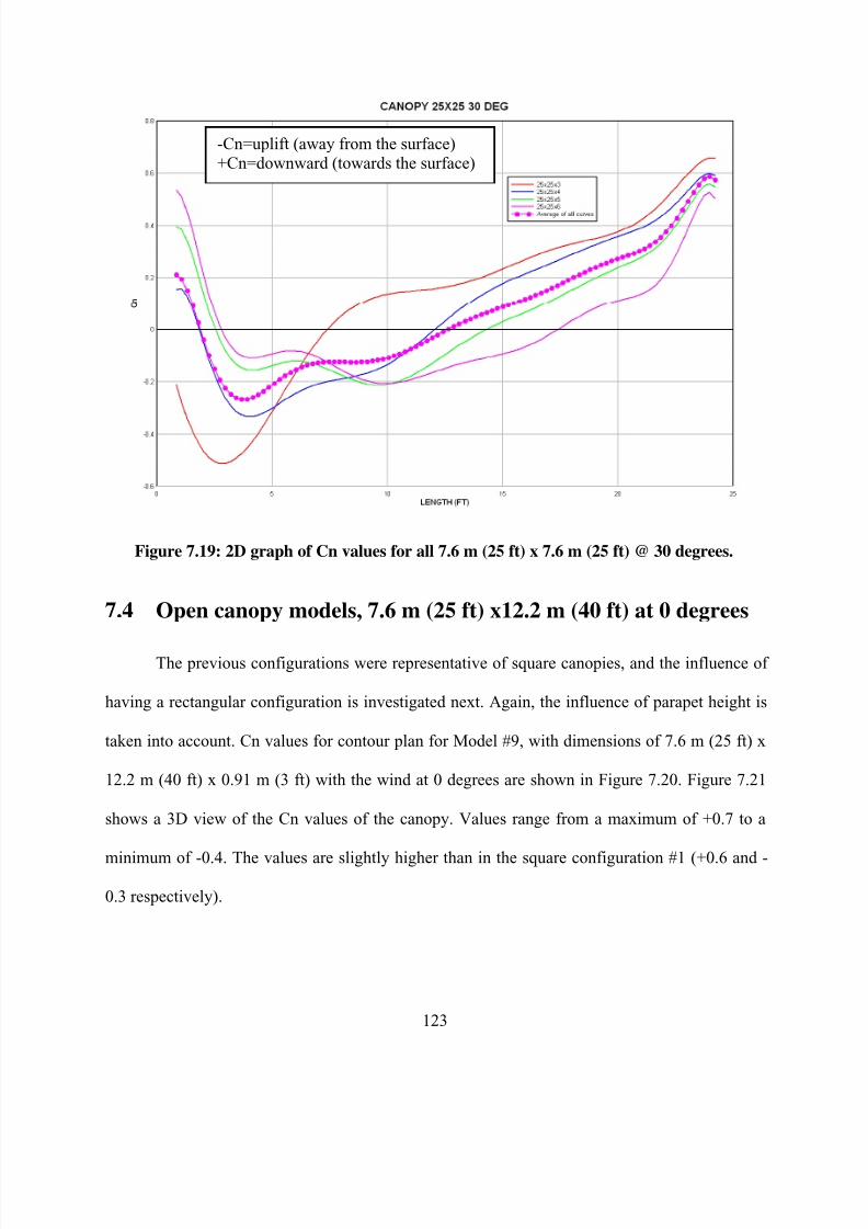
8/22/2019 Open Canopy Wind With Parapets
http://slidepdf.com/reader/full/open-canopy-wind-with-parapets 147/275
123
Figure 7.19: 2D graph of Cn values for all 7.6 m (25 ft) x 7.6 m (25 ft) @ 30 degrees.
7.4 Open canopy models, 7.6 m (25 ft) x12.2 m (40 ft) at 0 degrees
The previous configurations were representative of square canopies, and the influence of
having a rectangular configuration is investigated next. Again, the influence of parapet height is
taken into account. Cn values for contour plan for Model #9, with dimensions of 7.6 m (25 ft) x
12.2 m (40 ft) x 0.91 m (3 ft) with the wind at 0 degrees are shown in Figure 7.20. Figure 7.21
shows a 3D view of the Cn values of the canopy. Values range from a maximum of +0.7 to a
minimum of -0.4. The values are slightly higher than in the square configuration #1 (+0.6 and -
0.3 respectively).
-Cn=uplift (away from the surface)+Cn=downward (towards the surface)
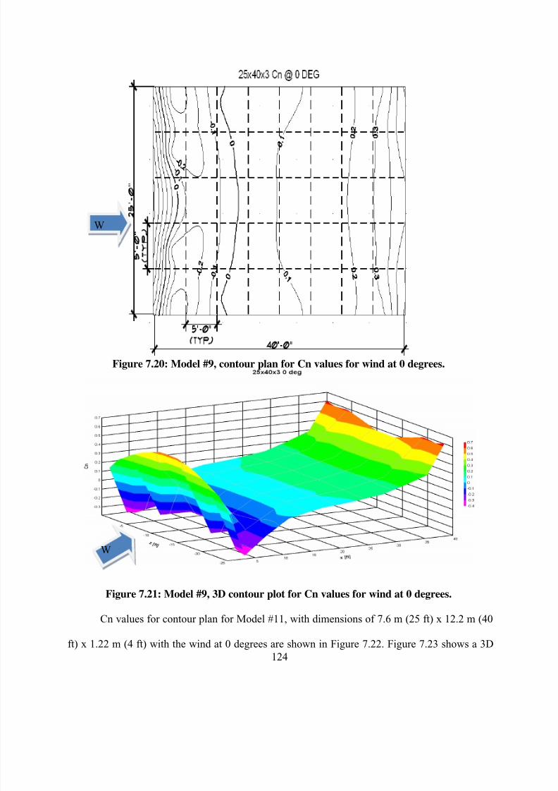
8/22/2019 Open Canopy Wind With Parapets
http://slidepdf.com/reader/full/open-canopy-wind-with-parapets 148/275
124
Figure 7.20: Model #9, contour plan for Cn values for wind at 0 degrees.
Figure 7.21: Model #9, 3D contour plot for Cn values for wind at 0 degrees.
Cn values for contour plan for Model #11, with dimensions of 7.6 m (25 ft) x 12.2 m (40
ft) x 1.22 m (4 ft) with the wind at 0 degrees are shown in Figure 7.22. Figure 7.23 shows a 3D
W
W

8/22/2019 Open Canopy Wind With Parapets
http://slidepdf.com/reader/full/open-canopy-wind-with-parapets 149/275
125
view of the Cn values of the canopy. Values range from a maximum of +0.7 to a minimum of -
0.3. In the square configuration, we reported extreme values of +0.8 and -0.3.
Figure 7.22: Model #11, contour plan for Cn values for wind at 0 degrees.
Figure 7.23: Model #11, 3D contour plot for Cn values for wind at 0 degrees.
W
W
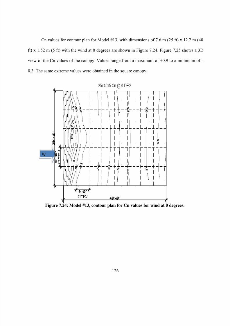
8/22/2019 Open Canopy Wind With Parapets
http://slidepdf.com/reader/full/open-canopy-wind-with-parapets 150/275
126
Cn values for contour plan for Model #13, with dimensions of 7.6 m (25 ft) x 12.2 m (40
ft) x 1.52 m (5 ft) with the wind at 0 degrees are shown in Figure 7.24. Figure 7.25 shows a 3D
view of the Cn values of the canopy. Values range from a maximum of +0.9 to a minimum of -
0.3. The same extreme values were obtained in the square canopy.
Figure 7.24: Model #13, contour plan for Cn values for wind at 0 degrees.
W
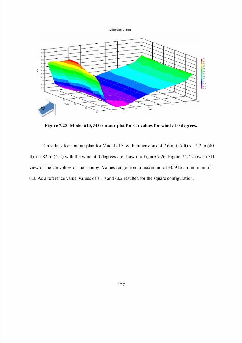
8/22/2019 Open Canopy Wind With Parapets
http://slidepdf.com/reader/full/open-canopy-wind-with-parapets 151/275
127
Figure 7.25: Model #13, 3D contour plot for Cn values for wind at 0 degrees.
Cn values for contour plan for Model #15, with dimensions of 7.6 m (25 ft) x 12.2 m (40
ft) x 1.82 m (6 ft) with the wind at 0 degrees are shown in Figure 7.26. Figure 7.27 shows a 3D
view of the Cn values of the canopy. Values range from a maximum of +0.9 to a minimum of -
0.3. As a reference value, values of +1.0 and -0.2 resulted for the square configuration.
W
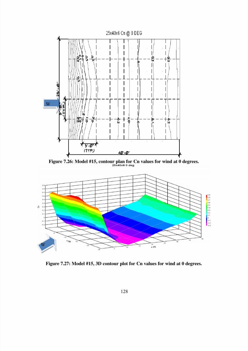
8/22/2019 Open Canopy Wind With Parapets
http://slidepdf.com/reader/full/open-canopy-wind-with-parapets 152/275
128
Figure 7.26: Model #15, contour plan for Cn values for wind at 0 degrees.
Figure 7.27: Model #15, 3D contour plot for Cn values for wind at 0 degrees.
W
W
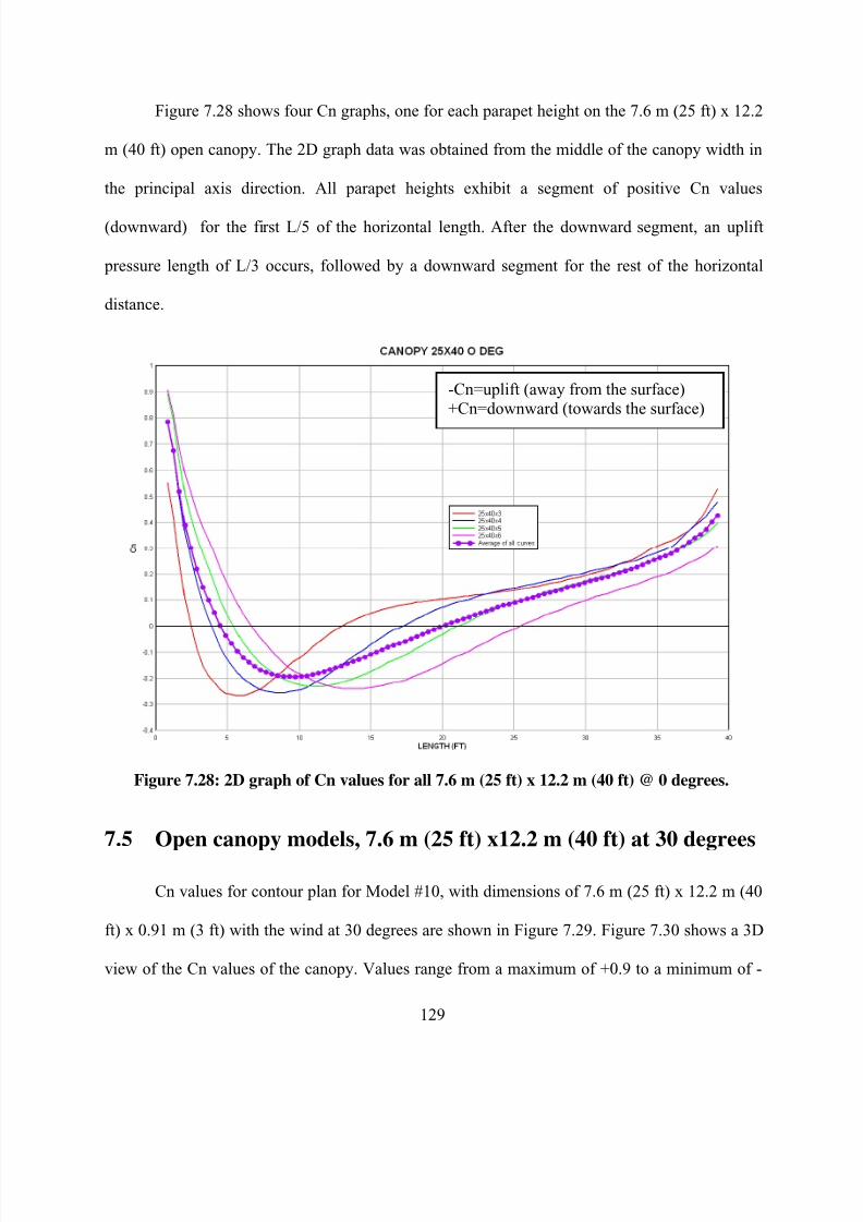
8/22/2019 Open Canopy Wind With Parapets
http://slidepdf.com/reader/full/open-canopy-wind-with-parapets 153/275
129
Figure 7.28 shows four Cn graphs, one for each parapet height on the 7.6 m (25 ft) x 12.2
m (40 ft) open canopy. The 2D graph data was obtained from the middle of the canopy width in
the principal axis direction. All parapet heights exhibit a segment of positive Cn values
(downward) for the first L/5 of the horizontal length. After the downward segment, an uplift
pressure length of L/3 occurs, followed by a downward segment for the rest of the horizontal
distance.
Figure 7.28: 2D graph of Cn values for all 7.6 m (25 ft) x 12.2 m (40 ft) @ 0 degrees.
7.5 Open canopy models, 7.6 m (25 ft) x12.2 m (40 ft) at 30 degrees
Cn values for contour plan for Model #10, with dimensions of 7.6 m (25 ft) x 12.2 m (40
ft) x 0.91 m (3 ft) with the wind at 30 degrees are shown in Figure 7.29. Figure 7.30 shows a 3D
view of the Cn values of the canopy. Values range from a maximum of +0.9 to a minimum of -
-Cn=uplift (away from the surface)+Cn=downward (towards the surface)

8/22/2019 Open Canopy Wind With Parapets
http://slidepdf.com/reader/full/open-canopy-wind-with-parapets 154/275
130
0.7. The values are slightly higher than in the square configuration #2 (+0.7 and -0.4
respectively).
Figure 7.29: Model #10, contour plan for Cn values for wind at 30 degrees.
W
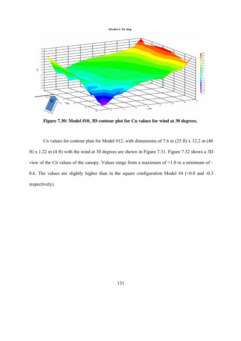
8/22/2019 Open Canopy Wind With Parapets
http://slidepdf.com/reader/full/open-canopy-wind-with-parapets 155/275
131
Figure 7.30: Model #10, 3D contour plot for Cn values for wind at 30 degrees.
Cn values for contour plan for Model #12, with dimensions of 7.6 m (25 ft) x 12.2 m (40
ft) x 1.22 m (4 ft) with the wind at 30 degrees are shown in Figure 7.31. Figure 7.32 shows a 3D
view of the Cn values of the canopy. Values range from a maximum of +1.0 to a minimum of -
0.6. The values are slightly higher than in the square configuration Model #4 (+0.8 and -0.3
respectively).
W

8/22/2019 Open Canopy Wind With Parapets
http://slidepdf.com/reader/full/open-canopy-wind-with-parapets 156/275
132
Figure 7.31: Model #12, contour plan for Cn values for wind at 30 degrees.
Figure 7.32: Model #12, 3D contour plot for Cn values for wind at 30 degrees.
W
W
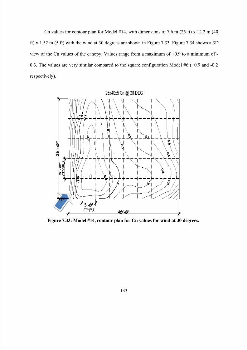
8/22/2019 Open Canopy Wind With Parapets
http://slidepdf.com/reader/full/open-canopy-wind-with-parapets 157/275
133
Cn values for contour plan for Model #14, with dimensions of 7.6 m (25 ft) x 12.2 m (40
ft) x 1.52 m (5 ft) with the wind at 30 degrees are shown in Figure 7.33. Figure 7.34 shows a 3D
view of the Cn values of the canopy. Values range from a maximum of +0.9 to a minimum of -
0.3. The values are very similar compared to the square configuration Model #6 (+0.9 and -0.2
respectively).
Figure 7.33: Model #14, contour plan for Cn values for wind at 30 degrees.
W
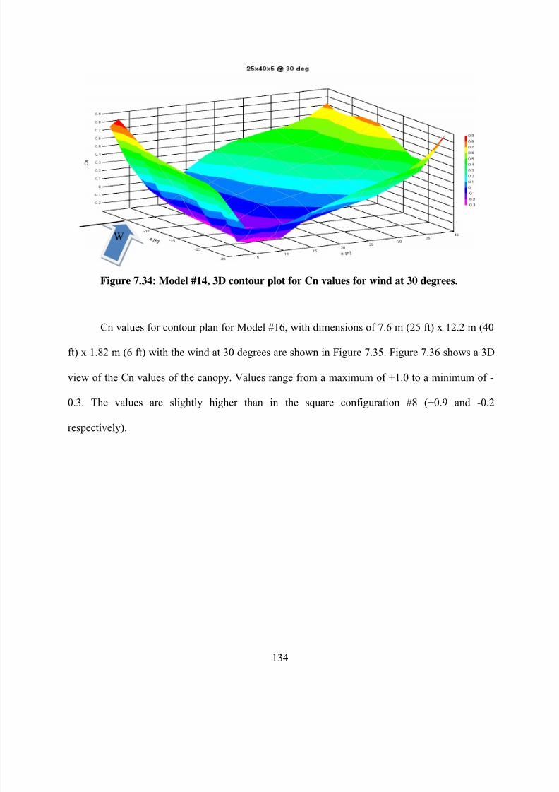
8/22/2019 Open Canopy Wind With Parapets
http://slidepdf.com/reader/full/open-canopy-wind-with-parapets 158/275
134
Figure 7.34: Model #14, 3D contour plot for Cn values for wind at 30 degrees.
Cn values for contour plan for Model #16, with dimensions of 7.6 m (25 ft) x 12.2 m (40
ft) x 1.82 m (6 ft) with the wind at 30 degrees are shown in Figure 7.35. Figure 7.36 shows a 3D
view of the Cn values of the canopy. Values range from a maximum of +1.0 to a minimum of -
0.3. The values are slightly higher than in the square configuration #8 (+0.9 and -0.2
respectively).
W

8/22/2019 Open Canopy Wind With Parapets
http://slidepdf.com/reader/full/open-canopy-wind-with-parapets 159/275
135
Figure 7.35: Model #16, contour plan for Cn values for wind at 30 degrees.
Figure 7.36: Model #16, 3D contour plot for Cn values for wind at 30 degrees.
W
W

8/22/2019 Open Canopy Wind With Parapets
http://slidepdf.com/reader/full/open-canopy-wind-with-parapets 160/275
136
Figure 7.37 shows four Cn graphs, one for each parapet height on the 7.6 m (25 ft) x 12.2
m (40 ft) open canopy. The 2D graph data was obtained from the middle of the canopy width in
the angle of the applied wind, in these case thirty (30) degrees from the principal axis direction.
All parapet height exhibits on the graph a segment of positive and negative Cn values.
Depending on the parapet height, downward and uplift pressure is reflected. This is shown on the
first L/5, except the parapet height of 0.91 m (3 ft) and 1.22 m (4 ft), which were all negative Cn
values. After the downward and uplift segment, an uplift pressure length of L/3 occurs followed
by a downward pressure for the rest of the horizontal distance.
Figure 7.37: Graph of Cn values for all 7.6 m (25 ft) x 12.2 m (40 ft) @ 30 degrees.
-Cn=uplift (away from the surface)+Cn=downward (towards the surface)

8/22/2019 Open Canopy Wind With Parapets
http://slidepdf.com/reader/full/open-canopy-wind-with-parapets 161/275
137
7.6 Open canopy models, 7.6 m (25 ft) x15.2 m (50 ft) at 0 degrees
An even longer canopy in the transverse direction is investigated in this section, in which
the length is increased to 50 ft. Cn values for contour plan for Model #17, with dimensions of 7.6
m (25 ft) x 15.2 m (50 ft) x 0.91 m (3 ft) with the wind at 0 degrees are shown in Figure 7.38.
Figure 7.39 shows a 3D view of the Cn values of the canopy. Values range from a maximum of
+0.7 to a minimum of -0.4. (Same as in Model #9).
Figure 7.38: Model #17, contour plan for Cn values for wind at 0 degrees.
W

8/22/2019 Open Canopy Wind With Parapets
http://slidepdf.com/reader/full/open-canopy-wind-with-parapets 162/275
138
Figure 7.39: Model #17, 3D contour plot for Cn values for wind at 0 degrees.
Cn values for contour plan for Model #19, with dimensions of 7.6 m (25 ft) x 15.2 m (50 ft) x
1.22 m (4 ft) with the wind at 0 degrees are shown in Figure 7.40. Figure 7.41 shows a 3D view
of the Cn values of the canopy. Values range from a maximum of +0.7 to a minimum of -0.4.
(Similar to Model #11).
W
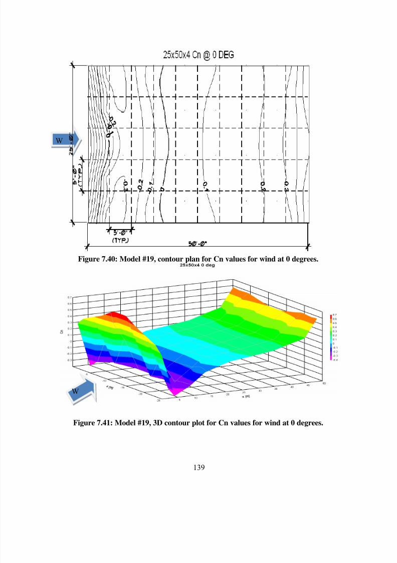
8/22/2019 Open Canopy Wind With Parapets
http://slidepdf.com/reader/full/open-canopy-wind-with-parapets 163/275
139
Figure 7.40: Model #19, contour plan for Cn values for wind at 0 degrees.
Figure 7.41: Model #19, 3D contour plot for Cn values for wind at 0 degrees.
W
W
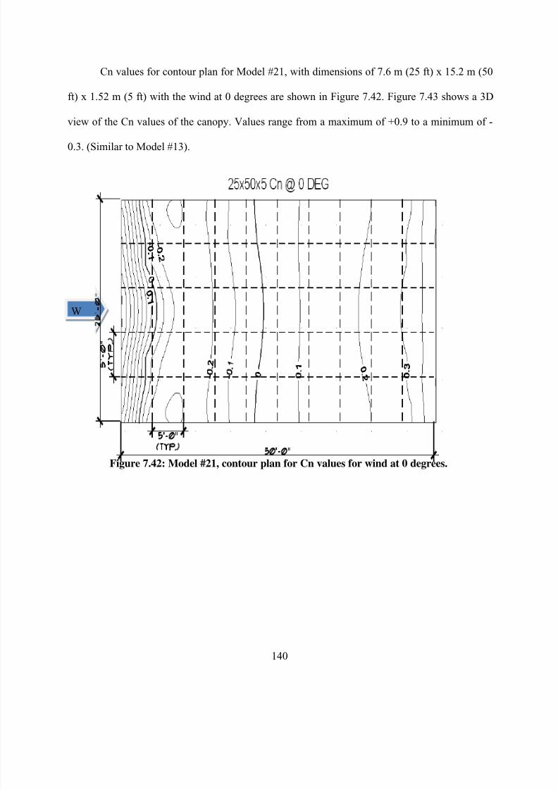
8/22/2019 Open Canopy Wind With Parapets
http://slidepdf.com/reader/full/open-canopy-wind-with-parapets 164/275
140
Cn values for contour plan for Model #21, with dimensions of 7.6 m (25 ft) x 15.2 m (50
ft) x 1.52 m (5 ft) with the wind at 0 degrees are shown in Figure 7.42. Figure 7.43 shows a 3D
view of the Cn values of the canopy. Values range from a maximum of +0.9 to a minimum of -
0.3. (Similar to Model #13).
Figure 7.42: Model #21, contour plan for Cn values for wind at 0 degrees.
W
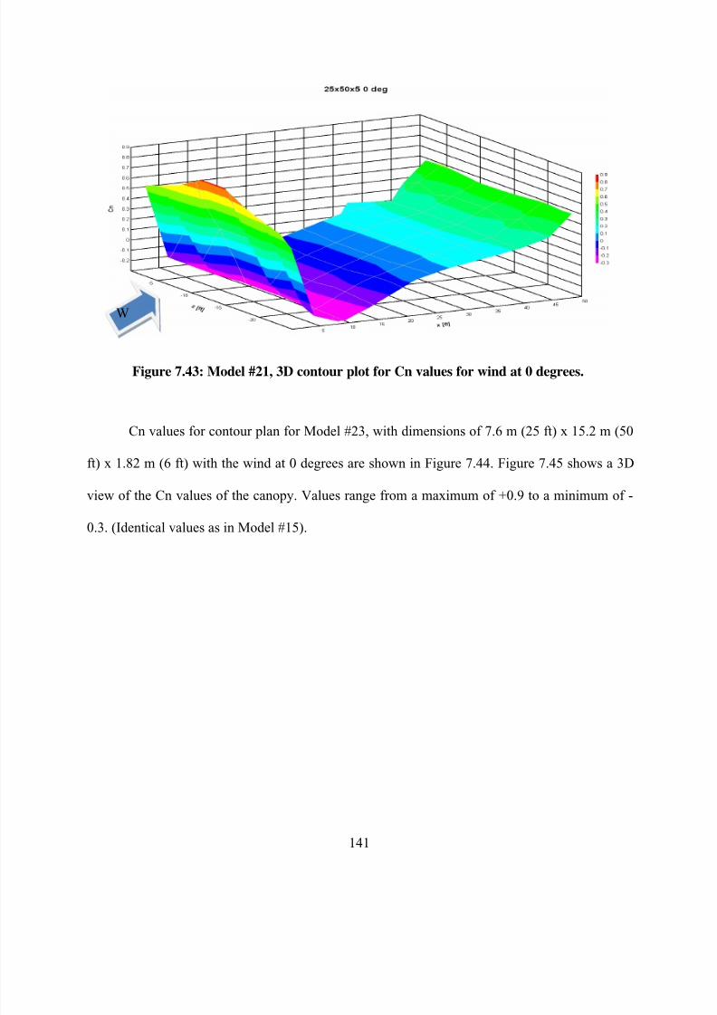
8/22/2019 Open Canopy Wind With Parapets
http://slidepdf.com/reader/full/open-canopy-wind-with-parapets 165/275
141
Figure 7.43: Model #21, 3D contour plot for Cn values for wind at 0 degrees.
Cn values for contour plan for Model #23, with dimensions of 7.6 m (25 ft) x 15.2 m (50
ft) x 1.82 m (6 ft) with the wind at 0 degrees are shown in Figure 7.44. Figure 7.45 shows a 3D
view of the Cn values of the canopy. Values range from a maximum of +0.9 to a minimum of -
0.3. (Identical values as in Model #15).
W
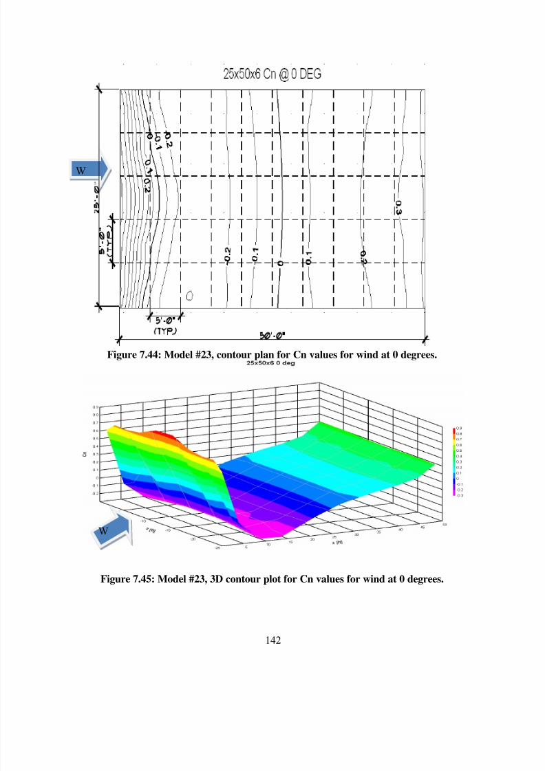
8/22/2019 Open Canopy Wind With Parapets
http://slidepdf.com/reader/full/open-canopy-wind-with-parapets 166/275
142
Figure 7.44: Model #23, contour plan for Cn values for wind at 0 degrees.
Figure 7.45: Model #23, 3D contour plot for Cn values for wind at 0 degrees.
W
W

8/22/2019 Open Canopy Wind With Parapets
http://slidepdf.com/reader/full/open-canopy-wind-with-parapets 167/275
143
Figure 7.46 shows four Cn graphs, one for each parapet height on the 7.6 m (25 ft) x 15.2
m (50 ft) open canopy. The 2D graph data was obtained from the middle of the canopy width in
the principal axis direction. All parapet height exhibits on the graph a segment of positive Cn
values (downward) for the first L/5 of the horizontal length. After the downward segment, an
uplift pressure length of L/3 occurs, followed by a downward for the rest of the horizontal
distance. The results computed for the canopy with 50 ft in the transverse direction are almost
identical to those computed for the 40 ft canopy.
Figure 7.46: 2D graph of Cn values for all 7.6 m (25 ft) x 15.2 m (50 ft) @ 0 degrees.
-Cn=uplift (away from the surface)
+Cn=downward (towards the surface)
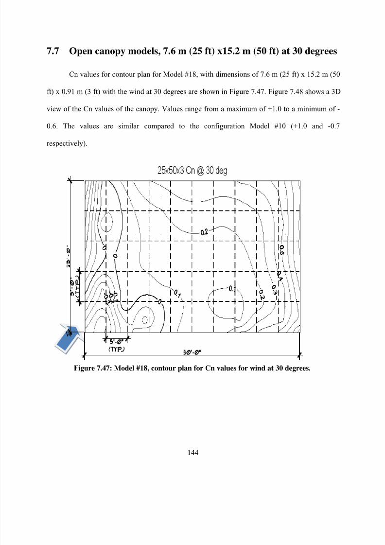
8/22/2019 Open Canopy Wind With Parapets
http://slidepdf.com/reader/full/open-canopy-wind-with-parapets 168/275
144
7.7 Open canopy models, 7.6 m (25 ft) x15.2 m (50 ft) at 30 degrees
Cn values for contour plan for Model #18, with dimensions of 7.6 m (25 ft) x 15.2 m (50
ft) x 0.91 m (3 ft) with the wind at 30 degrees are shown in Figure 7.47. Figure 7.48 shows a 3D
view of the Cn values of the canopy. Values range from a maximum of +1.0 to a minimum of -
0.6. The values are similar compared to the configuration Model #10 (+1.0 and -0.7
respectively).
Figure 7.47: Model #18, contour plan for Cn values for wind at 30 degrees.
W
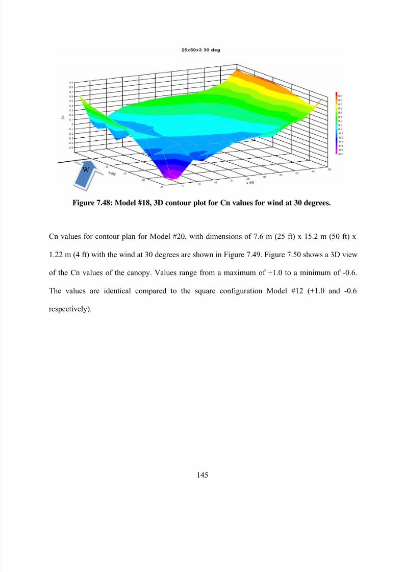
8/22/2019 Open Canopy Wind With Parapets
http://slidepdf.com/reader/full/open-canopy-wind-with-parapets 169/275
145
Figure 7.48: Model #18, 3D contour plot for Cn values for wind at 30 degrees.
Cn values for contour plan for Model #20, with dimensions of 7.6 m (25 ft) x 15.2 m (50 ft) x
1.22 m (4 ft) with the wind at 30 degrees are shown in Figure 7.49. Figure 7.50 shows a 3D view
of the Cn values of the canopy. Values range from a maximum of +1.0 to a minimum of -0.6.
The values are identical compared to the square configuration Model #12 (+1.0 and -0.6
respectively).
W

8/22/2019 Open Canopy Wind With Parapets
http://slidepdf.com/reader/full/open-canopy-wind-with-parapets 170/275
146
Figure 7.49: Model #20, contour plan for Cn values for wind at 30 degrees.
Figure 7.50: Model #20, 3D contour plot for Cn values for wind at 30 degrees.
W
W

8/22/2019 Open Canopy Wind With Parapets
http://slidepdf.com/reader/full/open-canopy-wind-with-parapets 171/275
147
Cn values for contour plan for Model #22, with dimensions of 7.6 m (25 ft) x 15.2 m (50
ft) x 1.52 m (5 ft) with the wind at 30 degrees are shown in Figure 7.51. Figure 7.52 shows a 3D
view of the Cn values of the canopy. Values range from a maximum of +1.0 to a minimum of -
0.4. The values are very similar compared to the configuration Model #14 (+0.9 and -0.3
respectively).
Figure 7.51: Model #22, contour plan for Cn values for wind at 30 degrees.
W

8/22/2019 Open Canopy Wind With Parapets
http://slidepdf.com/reader/full/open-canopy-wind-with-parapets 172/275
148
Figure 7.52: Model #22, 3D contour plot for Cn values for wind at 30 degrees.
Cn values for contour plan for Model #24, with dimensions of 7.6 m (25 ft) x 15.2 m (50 ft) x
1.82 m (6 ft) with the wind at 30 degrees are shown in Figure 7.53. Figure 7.54 shows a 3D view
of the Cn values of the canopy. Values range from a maximum of +0.9 to a minimum of -0.3.
The values on the configuration Model #14 are +1.0 and -0.3 respectively.
W
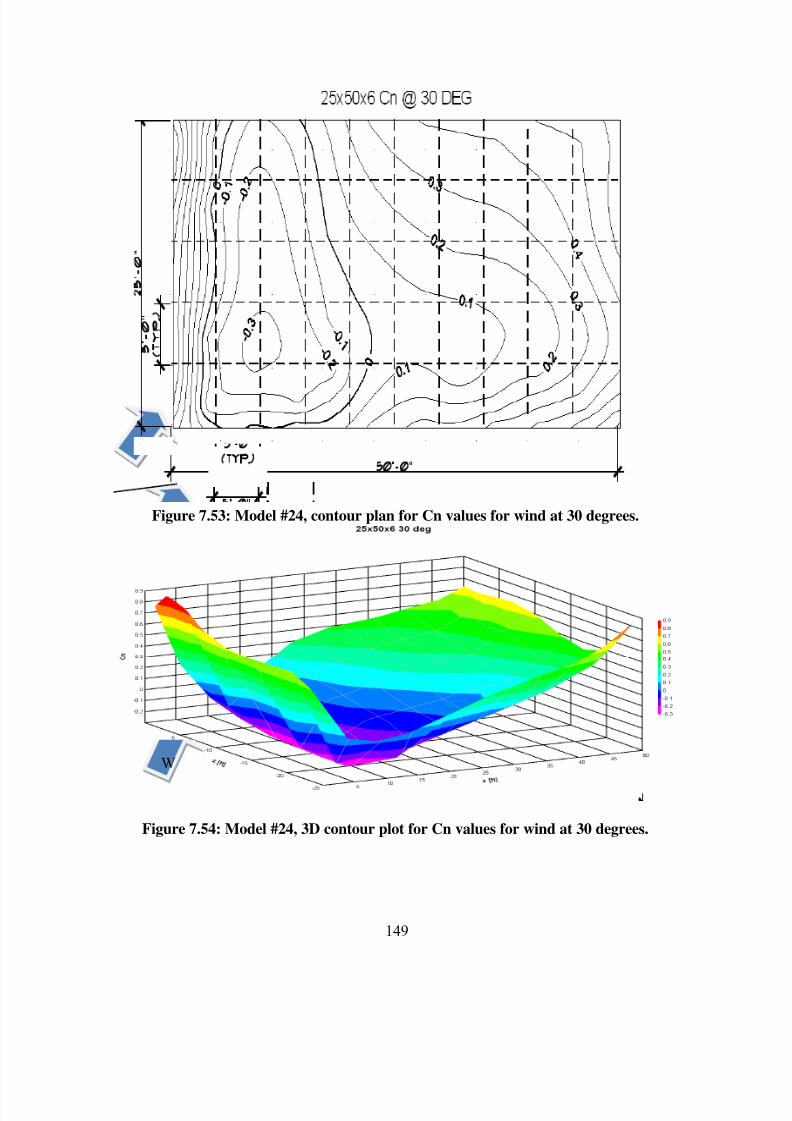
8/22/2019 Open Canopy Wind With Parapets
http://slidepdf.com/reader/full/open-canopy-wind-with-parapets 173/275
149
Figure 7.53: Model #24, contour plan for Cn values for wind at 30 degrees.
Figure 7.54: Model #24, 3D contour plot for Cn values for wind at 30 degrees.
W
W

8/22/2019 Open Canopy Wind With Parapets
http://slidepdf.com/reader/full/open-canopy-wind-with-parapets 174/275
150
Figure 7.55 shows four Cn graphs, one for each parapet height on the 7.6 m (25 ft) x 15.2
m (50 ft) open canopy. The 2D graph data was obtained at the center of the canopy width in the
angle of the applied wind, in this case, 30 degrees from the principal axis direction. All parapet
height exhibits on the graph a segment of positive and negative Cn values. Depending on the
parapet height, downward and uplift is reflected. This is shown on the first L/5, except the
parapet height of 0.91 m (3 ft) and 1.22 m (4 ft), which were all negative Cn values. After the
downward and uplift segment, an uplift pressure length of L/3 occurs followed by a downward
for the rest of the horizontal distance.
Figure 7.55: Graph of Cn values for all 7.6 m (25 ft) x 15.2 m (50 ft) @ 30 degrees.
7.8 Conclusions
Three canopy configurations were investigated in this chapter using CFD simulations, in
which wind incidence angle, parapet height, and transverse direction were changed to understand
pressure coefficient distributions. High changes are associated with parapet height, as expected,
-Cn=uplift (away from the surface)+Cn=downward (towards the surface)

8/22/2019 Open Canopy Wind With Parapets
http://slidepdf.com/reader/full/open-canopy-wind-with-parapets 175/275
151
as shown in Figures 7.10, 7.19, 7.28, 7.37, 7.46 and 7.55. The influence of wind direction is also
important in terms of values and pressure distributions, to visualize that it is necessary to
compare pairs of Figures, such as 7.10 and 7.19; 7.28 and 7.37; and 7.46 and 7.55. Finally, the
relative dimension of the canopy in plan has been investigated for a square configuration and two
rectangular ones. To visualize changes, one should compare Figures 7.10, 7.28 and 7.46; and
Figures 7.19, 7.37 and 7.55.
A warning should be made that differences between configurations used to compute
pressure values will lead the differences in structural response; however this is not a linear effect
and at this point in the thesis it is not clear how the detected differences will affect the response
of the structure. This the subject of Chapter 8.

8/22/2019 Open Canopy Wind With Parapets
http://slidepdf.com/reader/full/open-canopy-wind-with-parapets 176/275
152
CHAPTER 8. CASE STUDIES OF CANOPIES AND
COMPARISONS WITH FIELD EVIDENCE
8.1 Structural Analysis
From the point of view of this research, the structural analysis of open canopies that
suffered the effect of wind forces is very important for several reasons. First, a structural analysis
based on the previous pressure coefficients derived in this research work is extremely useful in
order to validate the proposed Cn wind coefficients on this type of structure. Second the
definitions of pressures due to wind make engineering sense in the context of structural analysis
and behavior. From the engineering point of view, the relevance of the pressure coefficients
depends on the performance of the structures affected by wind. For example, details of pressure
coefficients in given zones of a structure would not be relevant if the structural response is not
sensitive to those changes. Thus, we estimate wind speed data in order to make structural
analysis and improve structural behavior. The importance of wind pressures in the collapse of
canopies can be highlighted with reference to the multiple cases of failure identified following
hurricanes Katrina and Rita in 2005 (NIST, 2006). From reconnaissance missions to affected
areas by Hurricanes Katrina and Rita in 2005, four open canopies have been selected to perform
a structural analysis in this chapter. In the cases selected, wind velocity data was not available
and could only be estimated based on information available for neighboring areas. Current wind
velocity for the comparison of the selected case studies was estimated based on ASCE 7-05,
Figure 6-1A, page 34 that uses a 3 second gust speed. Wind speeds in Case 1, 2 and 4 have been
estimated to be about 130 mph. Wind speed in case 3 was estimated to be about 110 mph. The
wind velocities were used to obtain the wind pressures, and those pressures were used for the

8/22/2019 Open Canopy Wind With Parapets
http://slidepdf.com/reader/full/open-canopy-wind-with-parapets 177/275
153
structural analysis. This is a sequential methodology, in which the evaluation of wind pressures
is uncoupled for the structural response.
In order to propose and develop a methodology to analyze and calculate the structural
response of an open canopy, first we apply the wind pressure obtained from the Cn results on
Chapter 7. The structural effects of the applied wind pressures were analyzed considering two
main wind directions, at 0 and 30 degrees from the main horizontal axis. This procedure, in
which a detailed distribution of Cp values, based on contour levels is used, is called Method #1
and is similar to the methodology followed by Portela (2004). A second procedure, in which the
values from Method #1 are simplified, so that three zones of uniform pressure are identified with
their maximum values. Again, wind directions at 0 and 30 degrees were investigated. This
procedure was called Method #2. There is a third level of modeling attempted, which is based on
the same methodology employed by the ASCE 7-05, Section 6.5.13. The Cn values used on the
structural analysis for this method are the extreme values found in Chapter 7. This procedure was
called Method #3. Cn values vary from +1.2 to -0.6 and to +0.8 on this proposed method.
Typical proposed Cn values for Method #3 are summarized in Figure 8.1.
With the wind pressures obtained with all three methods, a structural analysis of the open
canopy was performed. The importance of doing structural analysis on case studies this is a
firsthand opportunity of analyzing a structure that has actually collapsed and see if that could be
anticipated (and prevented) with the use of the proposed Cn values.
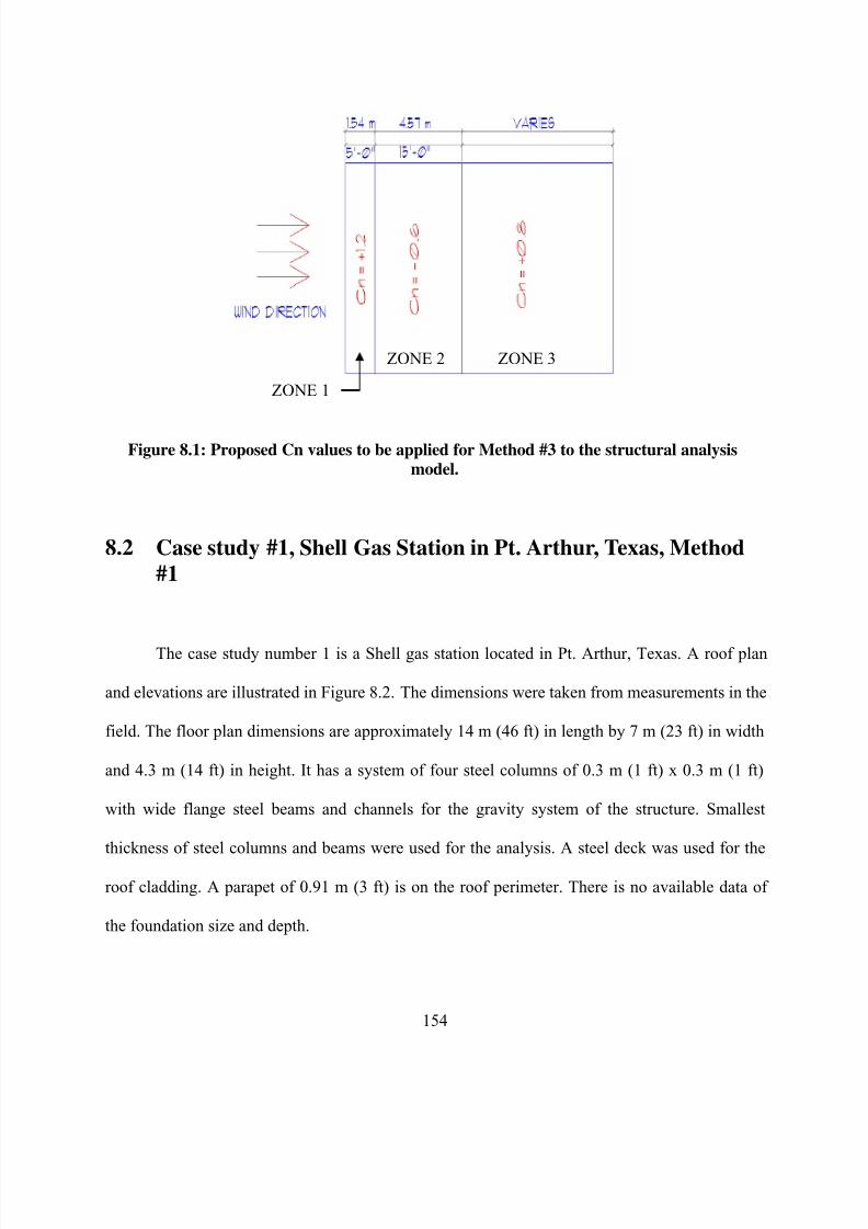
8/22/2019 Open Canopy Wind With Parapets
http://slidepdf.com/reader/full/open-canopy-wind-with-parapets 178/275
154
Figure 8.1: Proposed Cn values to be applied for Method #3 to the structural analysismodel.
8.2 Case study #1, Shell Gas Station in Pt. Arthur, Texas, Method
#1
The case study number 1 is a Shell gas station located in Pt. Arthur, Texas. A roof plan
and elevations are illustrated in Figure 8.2. The dimensions were taken from measurements in the
field. The floor plan dimensions are approximately 14 m (46 ft) in length by 7 m (23 ft) in width
and 4.3 m (14 ft) in height. It has a system of four steel columns of 0.3 m (1 ft) x 0.3 m (1 ft)
with wide flange steel beams and channels for the gravity system of the structure. Smallest
thickness of steel columns and beams were used for the analysis. A steel deck was used for the
roof cladding. A parapet of 0.91 m (3 ft) is on the roof perimeter. There is no available data of
the foundation size and depth.
ZONE 3ZONE 2
ZONE 1
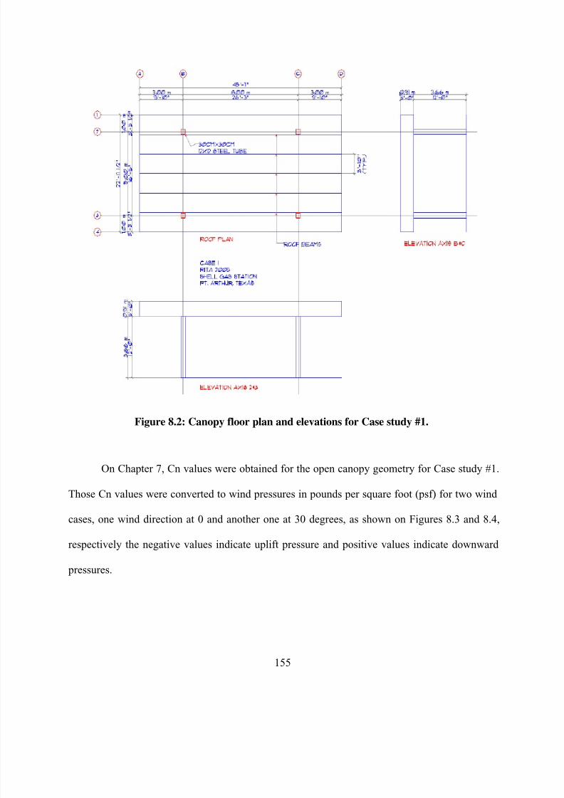
8/22/2019 Open Canopy Wind With Parapets
http://slidepdf.com/reader/full/open-canopy-wind-with-parapets 179/275
155
Figure 8.2: Canopy floor plan and elevations for Case study #1.
On Chapter 7, Cn values were obtained for the open canopy geometry for Case study #1.
Those Cn values were converted to wind pressures in pounds per square foot (psf) for two wind
cases, one wind direction at 0 and another one at 30 degrees, as shown on Figures 8.3 and 8.4,
respectively the negative values indicate uplift pressure and positive values indicate downward
pressures.
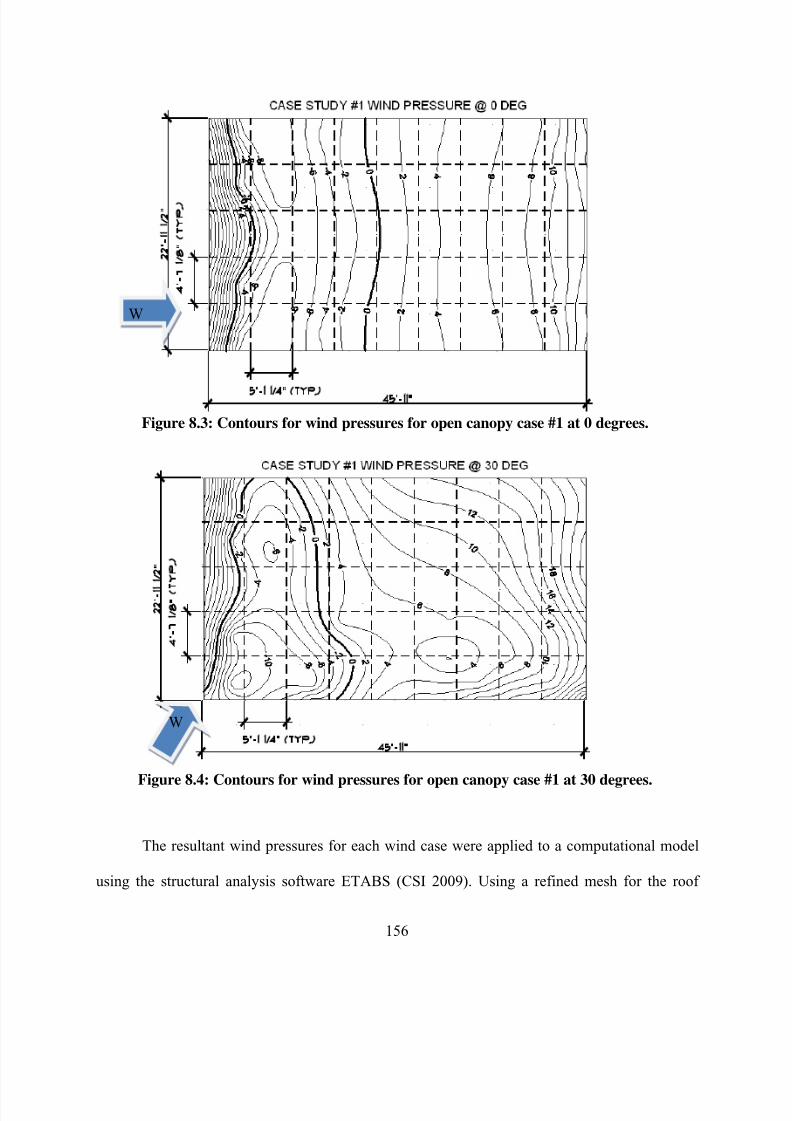
8/22/2019 Open Canopy Wind With Parapets
http://slidepdf.com/reader/full/open-canopy-wind-with-parapets 180/275
156
Figure 8.3: Contours for wind pressures for open canopy case #1 at 0 degrees.
Figure 8.4: Contours for wind pressures for open canopy case #1 at 30 degrees.
The resultant wind pressures for each wind case were applied to a computational model
using the structural analysis software ETABS (CSI 2009). Using a refined mesh for the roof
W
W

8/22/2019 Open Canopy Wind With Parapets
http://slidepdf.com/reader/full/open-canopy-wind-with-parapets 181/275
157
cladding, it was possible to input all the wind pressure values on the roof surface as shown on
Figures 8.5 and 8.6. The darker lines indicate the contours for wind pressures from the previous
figures.
Figure 8.5: Computer model with wind pressures applied to roof surface at 0 degrees.
Figure 8.6: Computer model with wind pressures applied to roof surface at 30 degrees.
The results of the applied wind load conditions at 0 and 30 degrees were obtained with
the use of ETABS, and Figure 8.7a and 8.7b show the deflected roof surface due to winds at 0
W
W
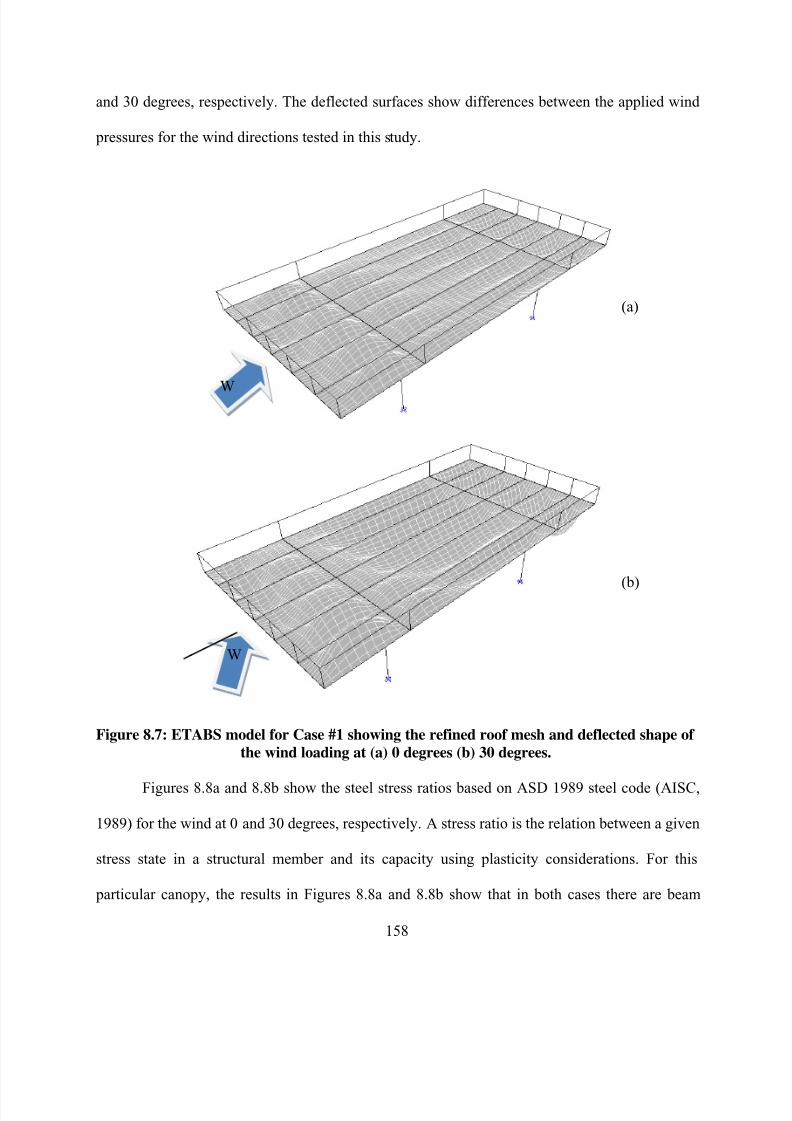
8/22/2019 Open Canopy Wind With Parapets
http://slidepdf.com/reader/full/open-canopy-wind-with-parapets 182/275
158
and 30 degrees, respectively. The deflected surfaces show differences between the applied wind
pressures for the wind directions tested in this study.
Figure 8.7: ETABS model for Case #1 showing the refined roof mesh and deflected shape of
the wind loading at (a) 0 degrees (b) 30 degrees.
Figures 8.8a and 8.8b show the steel stress ratios based on ASD 1989 steel code (AISC,
1989) for the wind at 0 and 30 degrees, respectively. A stress ratio is the relation between a given
stress state in a structural member and its capacity using plasticity considerations. For this
particular canopy, the results in Figures 8.8a and 8.8b show that in both cases there are beam
(a)
(b)
W
W

8/22/2019 Open Canopy Wind With Parapets
http://slidepdf.com/reader/full/open-canopy-wind-with-parapets 183/275
159
members with stress factors larger than 1. Wind direction at 30 degrees, produce higher stress
ratios than wind at 0 degrees. For example, the transverse beam on the leeward side of the roof
has a stress ratio of 1.515 for wind blowing at 0 degree, whereas for 30 degrees the ratio is 1.667,
that is, a 9.1 % difference. The long beams on the roof are also under conditions of severe stress,
showing values of 1.01 for 0° and 1.19 for 30°. The available evidence for this canopy, which
can be seen in Figures 8.18 to 8.22, indicate that the columns were still standing after the
structure failed and did not show signs of damage. The transverse beams, on the other hand, had
clearly failed, and this is in agreement with the computations carried out with Method #1 (also
with Methods #2 and #3, as will be seen next). The columns do not seem to be severely
compromised by the wind conditions considered. Method #1 has some disadvantages because the
wind load input for Method #1 is very complicated. A large number of elements need to be
included in the model to represent the contours and this has to be done by hand. Input has to be
done one by one, on each of the individual mesh elements, with the consequence that a total of
2400 roof shell elements were assigned wind loading pressures, one at a time. In addition, a
considerable amount of computational time is required to solve the model. The wind loading
computed and input, represents the calculated wind pressures on the open canopy, for a specific
parapet height. The need for a simpler design method is obvious and a second method, Method
#2 is proposed and investigated in the following section.

8/22/2019 Open Canopy Wind With Parapets
http://slidepdf.com/reader/full/open-canopy-wind-with-parapets 184/275
160
Figure 8.8: Structural steel results from ETABS for Case #1, showing members stressratios using Method #1 for (a) wind at 0 degrees (b) wind at 30 degrees.
(a)
(b)
W
W

8/22/2019 Open Canopy Wind With Parapets
http://slidepdf.com/reader/full/open-canopy-wind-with-parapets 185/275
161
8.3 Case study #1, Shell Gas Station in Pt. Arthur, Texas, Method
#2
Case study #1 was investigated using a simplified loading procedure, named Method #2.
It was proposed that instead of input all the contours on the roof surface, the new approach will
be to use the maximum wind pressure on the downward and uplift segments, from the extreme
wind pressures that were used in Method #1. This method simplifies the wind load input on a
structural model. Following recommendations in the literature for identifying the most critical
conditions, two wind directions were investigated, the wind at 0 degrees and 30 degrees. The
input wind pressures to be used on the structural model are shown on Figures 8.9 for 0° angle of
attack and Figure 8.10 for the 30° condition.
Figure 8.9: Roof canopy wind pressures for case #1, Method 2, wind at 0 degrees, + meansdownward pressure, - means uplift pressure.
ZONE 3ZONE 2
ZONE 1
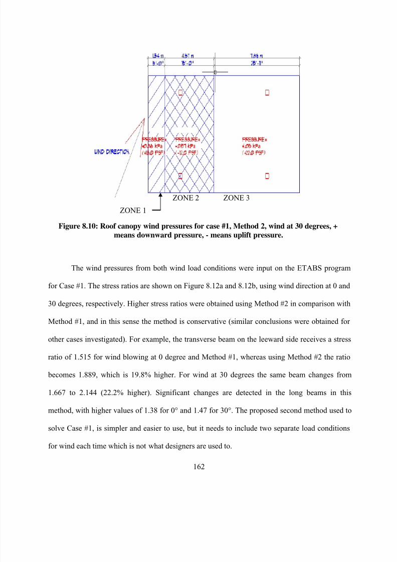
8/22/2019 Open Canopy Wind With Parapets
http://slidepdf.com/reader/full/open-canopy-wind-with-parapets 186/275
162
Figure 8.10: Roof canopy wind pressures for case #1, Method 2, wind at 30 degrees, +
means downward pressure, - means uplift pressure.
The wind pressures from both wind load conditions were input on the ETABS program
for Case #1. The stress ratios are shown on Figure 8.12a and 8.12b, using wind direction at 0 and
30 degrees, respectively. Higher stress ratios were obtained using Method #2 in comparison with
Method #1, and in this sense the method is conservative (similar conclusions were obtained for
other cases investigated). For example, the transverse beam on the leeward side receives a stress
ratio of 1.515 for wind blowing at 0 degree and Method #1, whereas using Method #2 the ratio
becomes 1.889, which is 19.8% higher. For wind at 30 degrees the same beam changes from
1.667 to 2.144 (22.2% higher). Significant changes are detected in the long beams in this
method, with higher values of 1.38 for 0° and 1.47 for 30°. The proposed second method used to
solve Case #1, is simpler and easier to use, but it needs to include two separate load conditions
for wind each time which is not what designers are used to.
ZONE 3ZONE 2
ZONE 1

8/22/2019 Open Canopy Wind With Parapets
http://slidepdf.com/reader/full/open-canopy-wind-with-parapets 187/275
163
Figure 8.11: Structural steel results from ETABS showing members stress ratios using
Method #2 for (a) wind at 0 degrees (b) wind at 30 degrees.
(a)
(b)
W
W

8/22/2019 Open Canopy Wind With Parapets
http://slidepdf.com/reader/full/open-canopy-wind-with-parapets 188/275
164
8.4 Case study #1, Shell Gas Station in Pt. Arthur, Texas, Method
#3
For the current case study, calculations following Method #3 were based on the
guidelines provided by ASCE 7-05. From the current results, the extreme Cn values from
Chapter 7 were selected. The calculated wind pressures and the resulting Cn values used are
shown in Figure 8.12. The mathematical procedure was performed with Maple, version 11
(Maplesoft, 2008), a symbolic manipulator program. The results of Figure 8.12 show values that
vary from +33.1 psf (+1.61 kPa) (downward pressure, zone 1), as well as -16.5 psf (-0.79 kPa)
(uplift pressure, zone 2) to +22 psf (1.05 kPa) (downward pressure, zone 3).
Parapet wind pressure values used for structural analysis are indicated in the computer
output shown in Figure 8.13. As previously described on Chapter 6, Cn values from the wind
tunnel and CFD simulation generally are in agreement. Wind pressure values were applied to the
structural model on the parapets. Wind pressures of 43.88 psf (2.1 kPa) in the windward
direction and 31.3 psf (1.5 kPa) in the leeward direction were applied to the structural model.
Wind direction was applied on both horizontal axis and wind pressures on the parapets are
applied at each wind direction. The proposed Method #3 combines the extreme values of the
wind loading of 0 and 30 degrees on the roof surface. It includes different parapet heights
calculated on Chapter 7.

8/22/2019 Open Canopy Wind With Parapets
http://slidepdf.com/reader/full/open-canopy-wind-with-parapets 189/275
165
Figure 8.12: Maple layout of Wind pressure calculations for Method #3, using proposed Cn
values and ASCE 7-05 procedure, Case# 1.
Proposed Cn values by
the author to be used for
Method 3, simplified design.
Wind speed mph at case#1 location
Wind pressure in
psf. H=horizontaldistance on the roof
surface.
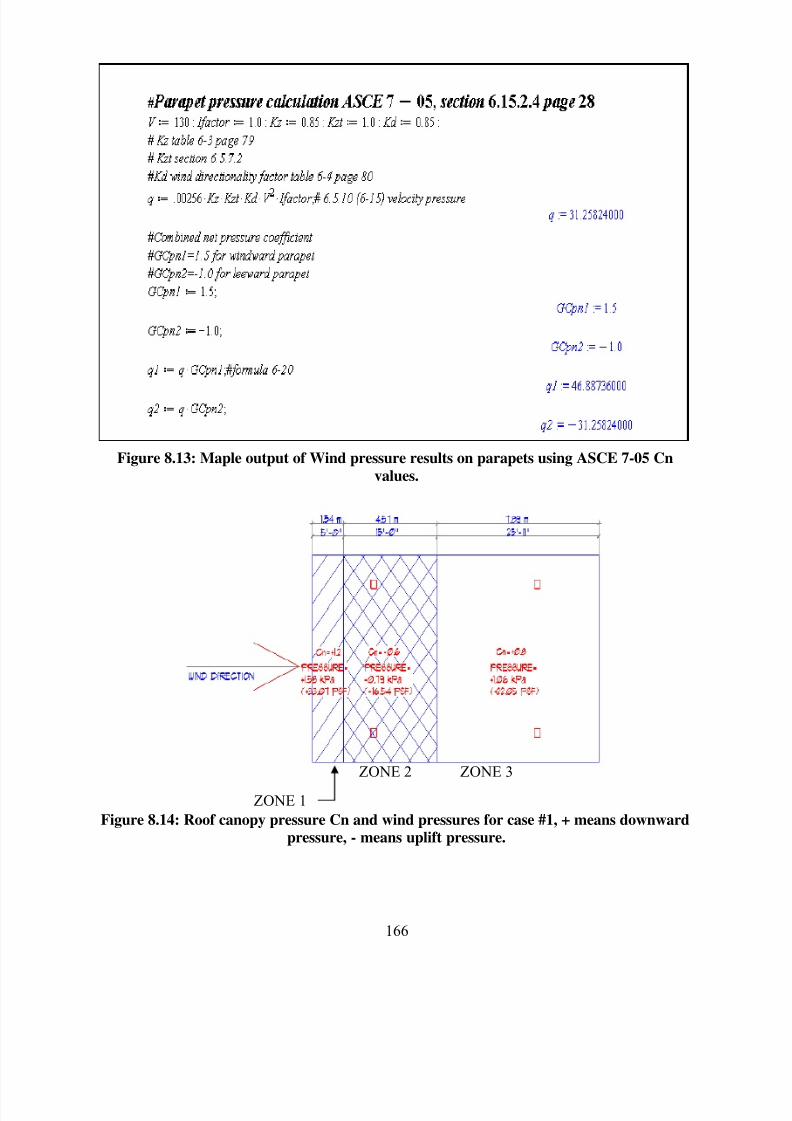
8/22/2019 Open Canopy Wind With Parapets
http://slidepdf.com/reader/full/open-canopy-wind-with-parapets 190/275
166
Figure 8.13: Maple output of Wind pressure results on parapets using ASCE 7-05 Cn
values.
Figure 8.14: Roof canopy pressure Cn and wind pressures for case #1, + means downwardpressure, - means uplift pressure.
ZONE 3ZONE 2
ZONE 1
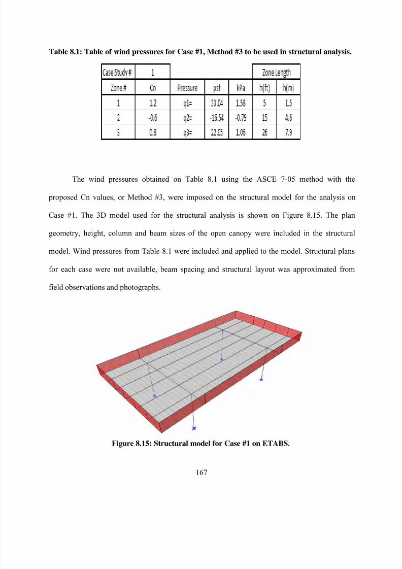
8/22/2019 Open Canopy Wind With Parapets
http://slidepdf.com/reader/full/open-canopy-wind-with-parapets 191/275
167
Table 8.1: Table of wind pressures for Case #1, Method #3 to be used in structural analysis.
The wind pressures obtained on Table 8.1 using the ASCE 7-05 method with the
proposed Cn values, or Method #3, were imposed on the structural model for the analysis on
Case #1. The 3D model used for the structural analysis is shown on Figure 8.15. The plan
geometry, height, column and beam sizes of the open canopy were included in the structural
model. Wind pressures from Table 8.1 were included and applied to the model. Structural plans
for each case were not available, beam spacing and structural layout was approximated from
field observations and photographs.
Figure 8.15: Structural model for Case #1 on ETABS.

8/22/2019 Open Canopy Wind With Parapets
http://slidepdf.com/reader/full/open-canopy-wind-with-parapets 192/275
168
Figure 8.16 show the deflected shape of the open canopy for Case #1 using Method #3.
The actual deflection on the roof edge is about 2.5” in the downward direction. Results from the
stress analysis are shown on Figure 8.17. Notice that only one wind case is considered here,
since the method combines the extreme values of 0° and 30° incident winds. The differences
between using Method #2 and #3 are small. For the leeward beam considered previously,
Method #2 leads to 1.889 (stress ratio at 0 degrees) and to 2.144 (stress ratio at 30 degrees),
whereas Method #3 (which combines both orientations) yields 2.131. The long beams on the roof
reach values of 1.5. Notice that Method #3 does not represent a lower bound in terms of stress
ratios, but is very close to that.
Figure 8.16: Structural model on ETABS showing deflected shape due to wind pressures.
Actual deflected
edge=2.5”,
downward
W

8/22/2019 Open Canopy Wind With Parapets
http://slidepdf.com/reader/full/open-canopy-wind-with-parapets 193/275
169
Figure 8.17: Structural model on ETABS showing overstress ratios on roof steel members.
Stress ratios on this structural model show overstressed ratios on the majority of the roof
beams. The graphical result shown is an envelope of all possible load combinations generated by
wind load cases, gravity loads and wind loads. The overstressed members in this case study
coincide with the failed steel elements shown in Figures 8.18 to 8.22. The failed elements
coincides with the analysis using a wind velocity as specified by the code, using the proposed Cn
values as suggested. All predictions need to be compared with evidence collected during site
visits, which are available in the form of photographs. If the Cn values proposed in this work had
been applied to carry out the original design, then, the main wind force resisting system
(MWFRS) should have been able to withstand the imposed wind pressures and to perform
satisfactory during hurricane Rita.
Therefore, Method #3 is simpler to use. It covers the extreme conditions from the wind
direction at 0 degrees and 30 degrees, and it includes the influence of different parapets heights.
Overstressed roof
members on
Model #1.
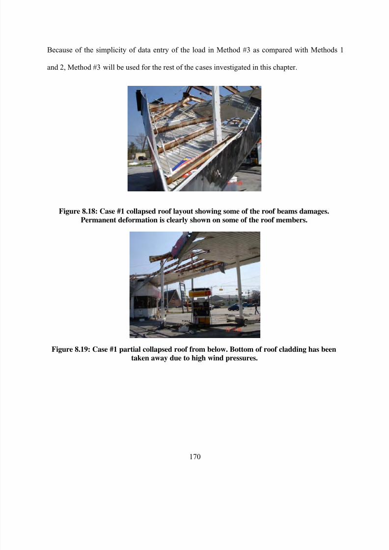
8/22/2019 Open Canopy Wind With Parapets
http://slidepdf.com/reader/full/open-canopy-wind-with-parapets 194/275
170
Because of the simplicity of data entry of the load in Method #3 as compared with Methods 1
and 2, Method #3 will be used for the rest of the cases investigated in this chapter.
Figure 8.18: Case #1 collapsed roof layout showing some of the roof beams damages.
Permanent deformation is clearly shown on some of the roof members.
Figure 8.19: Case #1 partial collapsed roof from below. Bottom of roof cladding has beentaken away due to high wind pressures.

8/22/2019 Open Canopy Wind With Parapets
http://slidepdf.com/reader/full/open-canopy-wind-with-parapets 195/275
171
Figure 8.20: Case #1 roof cladding and beam structural layout. Photograph showing
permanent deformation on roof members.
Figure 8.21: Case #1 transversal view of the deformed and collapsed roof.
Figure 8.22: Case #1, close up photograph of roof beams showing buckling and extremecorrosion damage.

8/22/2019 Open Canopy Wind With Parapets
http://slidepdf.com/reader/full/open-canopy-wind-with-parapets 196/275
172
8.5 Case study #2, Texaco Gas Station, Port Arthur, Texas
The case study number 2 is a Texaco gas station located in 39th Ave., Pt. Arthur, Texas.
Figure 8.23 shows the roof plan and elevations for Case #2. Measurements were taken directly
from the field. The floor plan dimensions are 6.1 m (20 ft) in width by 8.8 m (29 ft) in length and
4.3 m (14 ft) in heigth. The open canopy has a system of four steel columns of 0.3 m (1 ft)
diameter with steel beams and channels for the gravity system of the structure. Smallest
thickness of steel columns and beams were used for the analysis. A steel deck was used for the
roof cladding. A parapet of 0.91 m (3 ft) is on the roof perimeter. There is no data available for
the foundation size and depth.
For the current case study, calculations were based on Method #3, which uses the
guidelines provided by ASCE 7-05. From the current results, the Cn values from Chapter 7 were
selected. Refer to Figure 8.24 for calculated wind pressure results and Cn values used. As in
other cases, the calculations were done with Maple, and show values that vary from +33.1 psf
(+1.61 kPa) (downward pressure, zone 1), -16.5 psf (-0.79 kPa) (uplift pressure, zone 2) to +22
psf (1.05 kPa) (downward pressure, zone 3).

8/22/2019 Open Canopy Wind With Parapets
http://slidepdf.com/reader/full/open-canopy-wind-with-parapets 197/275
173
Figure 8.23: Canopy floor plan and elevations for Case study #2.
Parapet wind pressure values used for structural analysis are shown on Figure 8.13. Wind
pressures of 43.88 psf (2.1 kPa) on the windward direction and 31.3 psf (1.5 kPa) on the leeward
direction were applied to the structural model. Wind direction was applied on both horizontal
axis and wind pressures on the parapets are applied at each wind direction.
The obtained wind pressures obtained and shown on Table 8.2 using the ASCE 7-05
method and the proposed Cn values from this thesis were imposed on the structural model for the
analysis on Case #2. Refer to Figure 8.26 for the 3D model used for the structural analysis of the

8/22/2019 Open Canopy Wind With Parapets
http://slidepdf.com/reader/full/open-canopy-wind-with-parapets 198/275
174
structure on Case #2. Open canopy plan geometry, height, column and beam sizes, were included
in the structural model. Wind pressures from Table 8.2 were included and applied to the model.
Stress ratios computed for the structural model show stress ratios values larger than one
on all steel columns (Figure 8.26). The graphical result shown in this figure is an envelope of all
possible load combinations generated by wind load cases, gravity loads and wind loads, and
evaluated using the steel design code (AISC 1989). Unlike what was obtained in our Case study
#1, in which the roof beams reached failure, the columns are the weak elements in Case study #2,
whereas all roof elements are in safe state. The overstressed members in this case study are the
same as the failed steel elements shown on Figure 8.28 to 8.32. The columns used on this open
canopy are very slender, and just by looking at the dimensions, only six inches in diameter.
Therefore, it does not surprise the author, that they failed so drastically under imposed wind
pressures. Plastic hinges are observed in all four columns, and because of the advanced state of
deterioration is seems that failure occur for loads (and wind velocities) lower than those
considered in the analysis.
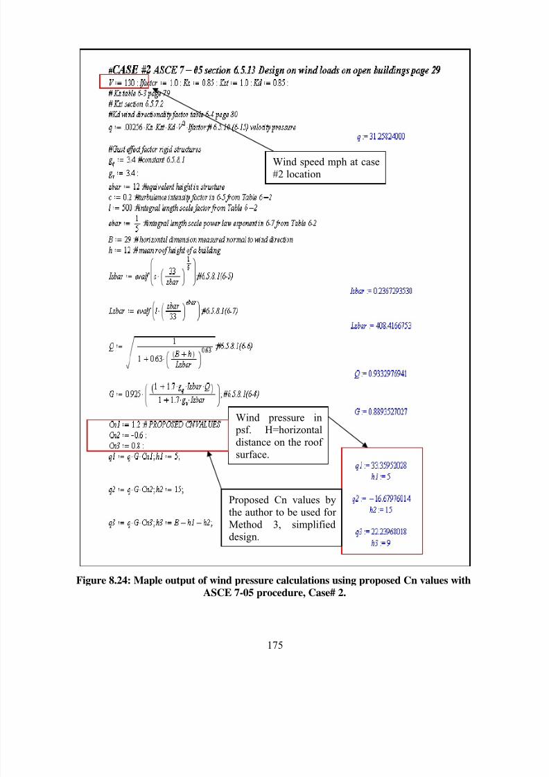
8/22/2019 Open Canopy Wind With Parapets
http://slidepdf.com/reader/full/open-canopy-wind-with-parapets 199/275
175
Figure 8.24: Maple output of wind pressure calculations using proposed Cn values with
ASCE 7-05 procedure, Case# 2.
Wind speed mph at case
#2 location
Wind pressure in psf. H=horizontal
distance on the roof
surface.
Proposed Cn values by
the author to be used for
Method 3, simplified design.

8/22/2019 Open Canopy Wind With Parapets
http://slidepdf.com/reader/full/open-canopy-wind-with-parapets 200/275
176
Figure 8.25: Roof canopy pressure Cn and wind pressures for case #2, + means downwardpressure, - means uplift pressure.
Table 8.2: Table of wind pressures for Case #2 to be used in structural analysis.
ZONE 3ZONE 2
ZONE 1
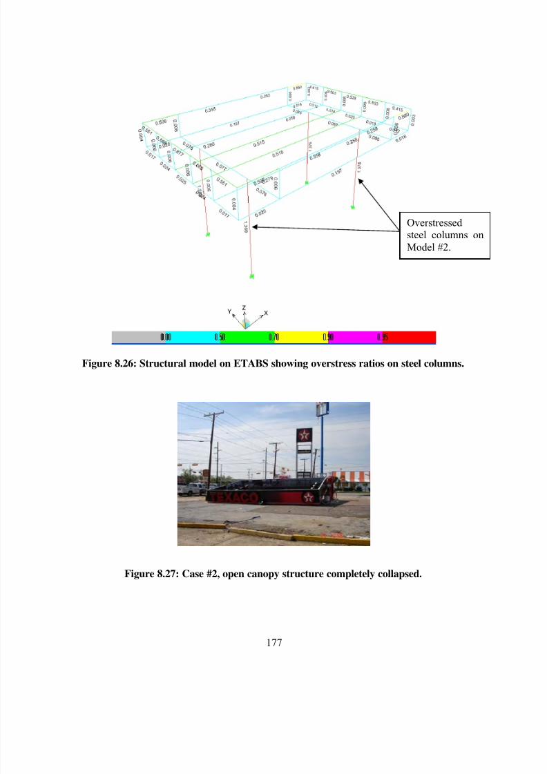
8/22/2019 Open Canopy Wind With Parapets
http://slidepdf.com/reader/full/open-canopy-wind-with-parapets 201/275
177
Figure 8.26: Structural model on ETABS showing overstress ratios on steel columns.
Figure 8.27: Case #2, open canopy structure completely collapsed.
Overstressed steel columns on
Model #2.

8/22/2019 Open Canopy Wind With Parapets
http://slidepdf.com/reader/full/open-canopy-wind-with-parapets 202/275
178
Figure 8.28: Case #2, photograph showing a buckled round steel column.
Figure 8.29: Case #2, closer photograph of the round steel column base.

8/22/2019 Open Canopy Wind With Parapets
http://slidepdf.com/reader/full/open-canopy-wind-with-parapets 203/275
179
Figure 8.30: Case #2, photograph showing the open canopy structure on top of the gas
pumps.
Figure 8.31: Case #2, photograph showing the roof beam layout.
8.6 Case study #3, Chevron Gas station, Vidor, Texas
The case study number 3 is a Chevron gas station located in Road 105 and HW 10,
Vidor, Texas. A roof plan and elevations are illustrated in Figure 8.32 and were taken from
measurements in the field. The floor plan dimensions are approximately 8.0 m (26 ft) in width by

8/22/2019 Open Canopy Wind With Parapets
http://slidepdf.com/reader/full/open-canopy-wind-with-parapets 204/275
180
12.2 m (40 ft) in length and 4.3 m (14 ft) in height. It has a system of two steel columns of 0.3 m
(1 ft) x 0.3 m (1 ft) with steel beams and channels for the gravity system of the structure.
Smallest thickness of steel columns and beams were used for the analysis. A steel deck was used
for the roof cladding. A parapet of 0.91 m (3 ft) is on the roof perimeter. There is no data
available concerning the foundation size and depth.
Figure 8.32: Canopy floor plan and elevations for Case study #3.
For the current case study, calculations are based on Method #3, which follows the
guidelines provided by ASCE 7-05. The calculated wind pressure results and used Cn values are
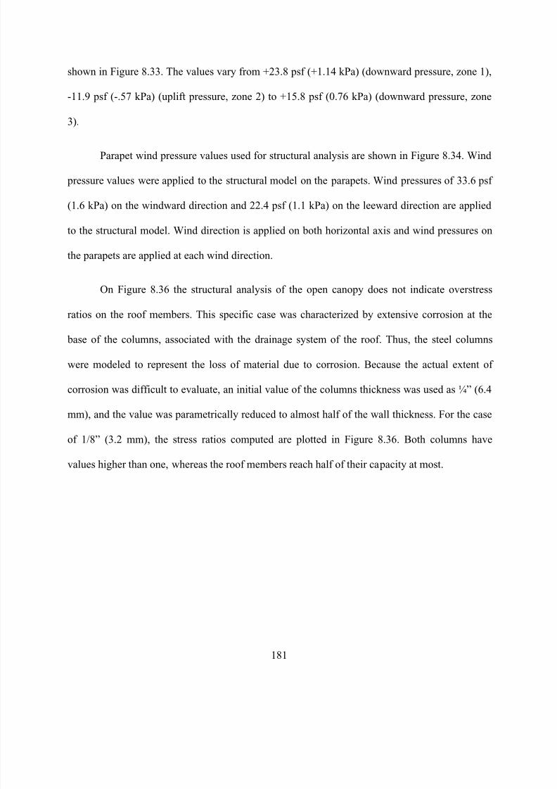
8/22/2019 Open Canopy Wind With Parapets
http://slidepdf.com/reader/full/open-canopy-wind-with-parapets 205/275
181
shown in Figure 8.33. The values vary from +23.8 psf (+1.14 kPa) (downward pressure, zone 1),
-11.9 psf (-.57 kPa) (uplift pressure, zone 2) to +15.8 psf (0.76 kPa) (downward pressure, zone
3).
Parapet wind pressure values used for structural analysis are shown in Figure 8.34. Wind
pressure values were applied to the structural model on the parapets. Wind pressures of 33.6 psf
(1.6 kPa) on the windward direction and 22.4 psf (1.1 kPa) on the leeward direction are applied
to the structural model. Wind direction is applied on both horizontal axis and wind pressures on
the parapets are applied at each wind direction.
On Figure 8.36 the structural analysis of the open canopy does not indicate overstress
ratios on the roof members. This specific case was characterized by extensive corrosion at the
base of the columns, associated with the drainage system of the roof. Thus, the steel columns
were modeled to represent the loss of material due to corrosion. Because the actual extent of
corrosion was difficult to evaluate, an initial value of the columns thickness was used as ¼” (6.4
mm), and the value was parametrically reduced to almost half of the wall thickness. For the case
of 1/8” (3.2 mm), the stress ratios computed are plotted in Figure 8.36. Both columns have
values higher than one, whereas the roof members reach half of their capacity at most.
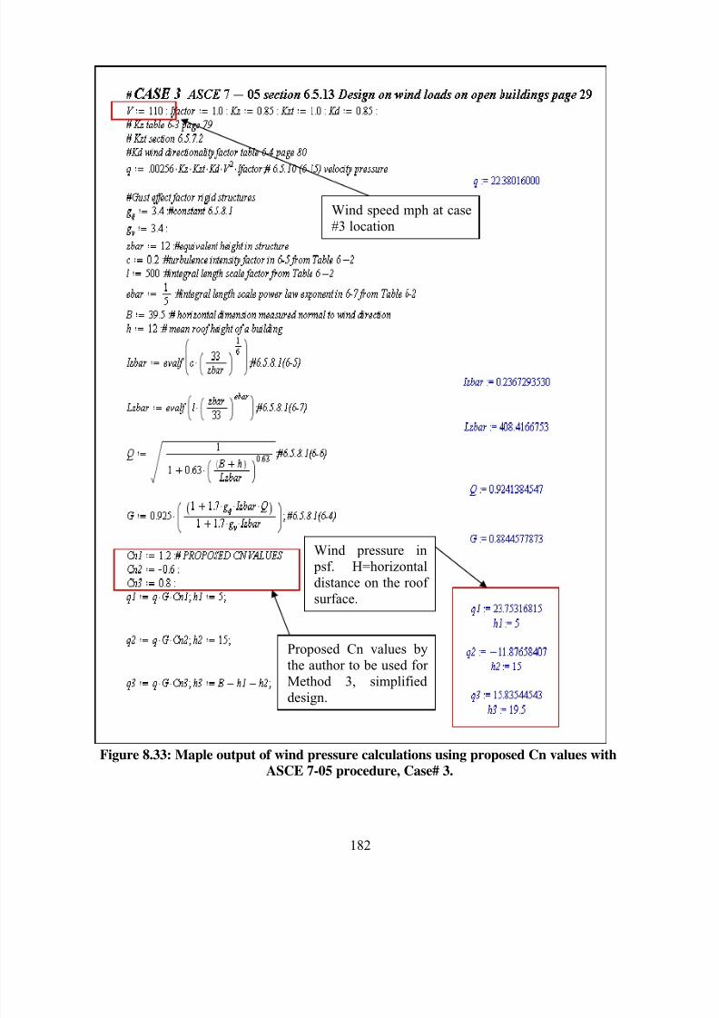
8/22/2019 Open Canopy Wind With Parapets
http://slidepdf.com/reader/full/open-canopy-wind-with-parapets 206/275
182
Figure 8.33: Maple output of wind pressure calculations using proposed Cn values withASCE 7-05 procedure, Case# 3.
Wind speed mph at case
#3 location
Wind pressure in
psf. H=horizontal
distance on the roof
surface.
Proposed Cn values by
the author to be used for
Method 3, simplified
design.

8/22/2019 Open Canopy Wind With Parapets
http://slidepdf.com/reader/full/open-canopy-wind-with-parapets 207/275
183
Figure 8.34: Maple output of wind pressure results on parapets using ASCE 7-05 Cn values
Figure 8.35: Roof canopy pressure Cn and wind pressures for case #3, + means downwardpressure, - means uplift pressure.
ZONE 3ZONE 2ZONE 1

8/22/2019 Open Canopy Wind With Parapets
http://slidepdf.com/reader/full/open-canopy-wind-with-parapets 208/275
184
Table 8.3: Table of wind pressures for Case #3 to be used in structural analysis.
Figure 8.36: Structural model on ETABS showing overstress ratios on roof steel membersfor Case #3.
Figures 8.38 to 8.40 show the corrosion damage at the base of the steel columns, which is
believed to have triggered the collapse of the structure. The steel columns failed below their
stress capacity and even the complete structural layout remained intact after the failure of the
steel columns. It is remarkable that the whole superstructure, the MWFRS and the secondary
members, remained intact after the structure became upside down after the failure. Without the
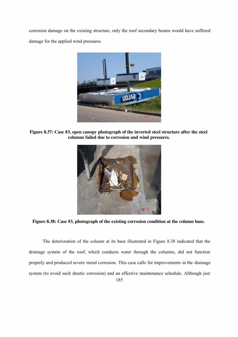
8/22/2019 Open Canopy Wind With Parapets
http://slidepdf.com/reader/full/open-canopy-wind-with-parapets 209/275
185
corrosion damage on the existing structure, only the roof secondary beams would have suffered
damage for the applied wind pressures.
Figure 8.37: Case #3, open canopy photograph of the inverted steel structure after the steel
columns failed due to corrosion and wind pressures.
Figure 8.38: Case #3, photograph of the existing corrosion condition at the column base.
The deterioration of the column at its base illustrated in Figure 8.38 indicated that the
drainage system of the roof, which conducts water through the columns, did not function
properly and produced severe metal corrosion. This case calls for improvements in the drainage
system (to avoid such drastic corrosion) and an effective maintenance schedule. Although just

8/22/2019 Open Canopy Wind With Parapets
http://slidepdf.com/reader/full/open-canopy-wind-with-parapets 210/275
186
one case involving corrosion was analyzed in this chapter, this pattern of deterioration was
observed in many cases during site visits.
Figure 8.39: Case #3, additional photograph of the inverted steel structure.
8.7 Case study #4, Exxon Gas station, Hillerbrandt, Texas
The case study number 4 is an Exxon gas station located in Road 365, Hillerbrandt,
Texas. A roof plan and elevations as illustrated in Figure 8.40 and were taken from field
measurements. The floor plan dimensions are approximately 9.8 m (32 ft) x 25.0 m (85 ft) x 4.3
m (14 ft). It has a system of four steel columns of 0.3 m (1 ft) x 0.3 m (1 ft) with steel beams and
channels for the gravity system of the structure. Smallest thickness of steel columns and beams
were used for the analysis. A steel deck was used for roof cladding. A parapet of 0.91 m (3 ft) is
on the roof perimeter. There is no data available for the foundation size and depth.

8/22/2019 Open Canopy Wind With Parapets
http://slidepdf.com/reader/full/open-canopy-wind-with-parapets 211/275
187
Figure 8.40: Canopy floor plan and elevations for Case study #4.
For the current case study, calculations are based on the guidelines provided by ASCE 7-
05, Method #3. Figure 8.41 shows the calculated wind pressures from the proposed Cn, with
values that varied from +33.1 psf (+1.61 kPa) (downward pressure, zone 1), -16.5 psf (-.79 kPa)
(uplift pressure, zone 2) to +22 psf (1.05 kPa) (downward pressure, zone 3).

8/22/2019 Open Canopy Wind With Parapets
http://slidepdf.com/reader/full/open-canopy-wind-with-parapets 212/275
188
Parapet wind pressure values used for structural analysis are shown on Figure 8.13. Wind
pressure values were applied to the structural model on the parapets. Wind pressures of 43.88 psf
(2.1 kPa) on the windward direction and 31.3 psf (1.5 kPa) on the leeward direction are applied
to the structural model. Wind direction is applied on both horizontal axis and wind pressures on
the parapets are applied at each wind direction.
Stress ratios larger than one on this structural model show overstressed ratios on all steel
columns. The values displayed in Figure 8.43 is an envelope of all possible load combinations
generated by wind load cases, gravity loads and wind loads, using steel design code (AISC
1989). As reference values, the maximum service of the column axial load is 17.1 kips and the
maximum service moment in the strong axis is 119 k-ft. The maximum ultimate column axial
load is 28.2 kips and the maximum ultimate moment in the strong axis is 154.5 k-ft.
In this particular case is very interesting to identify from the photographs the buckling of
the column flanges. The maximum capacity of the flanges before the local flange goes into
plastic deformation is 138.9 kips. From the computations, it seems that plastic hinge in one of the
local flanges has initially formed, causing the rotation and failure of all steel columns. The actual
computational model results using Method #3 produce results that are comparable to the failure
mechanism and loads that the actual structure suffered from wind forces. The overstressed
members in this case coincide with the failed steel column elements shown on Figure 8.45 to
8.48.

8/22/2019 Open Canopy Wind With Parapets
http://slidepdf.com/reader/full/open-canopy-wind-with-parapets 213/275
189
Figure 8.41: Maple output of wind pressure calculations using proposed Cn values withASCE 7-05 procedure, Case# 4.
Wind speed mph at case#4 location
Wind pressure in psf. H=horizontal
distance on the roof
surface.
Proposed Cn values by
the author to be used for Method 3, simplified
design.

8/22/2019 Open Canopy Wind With Parapets
http://slidepdf.com/reader/full/open-canopy-wind-with-parapets 214/275
190
Figure 8.42: Roof canopy pressure Cn and wind pressures for case #4, + means downwardpressure, - means uplift pressure.
Table 8.4: Table of wind pressures for Case #4 to be used in structural analysis.
ZONE 3ZONE 2ZONE 1

8/22/2019 Open Canopy Wind With Parapets
http://slidepdf.com/reader/full/open-canopy-wind-with-parapets 215/275
191
Figure 8.43: Structural model generated with ETABS showing overstress ratios on all steel
columns.
Figure 8.44: Case #4, photograph showing closer detail of the buckled steel columns.
Overstressed
steel columnson Model #4.

8/22/2019 Open Canopy Wind With Parapets
http://slidepdf.com/reader/full/open-canopy-wind-with-parapets 216/275
192
Figure 8.45: Case #4, photograph showing the collapsed steel columns.
Figure 8.46: Case #4, additional photograph of buckled steel columns. The photographshows the internal column flange.
Figure 8.47: Case #4, upper roof beam layout on the collapsed open canopy roof.

8/22/2019 Open Canopy Wind With Parapets
http://slidepdf.com/reader/full/open-canopy-wind-with-parapets 217/275
193
8.8 Conclusions drawn from the Case Studies
The Cn values obtained from wind tunnel experiments and CFD simulation were
obtained on Chapter 6. CFD simulations could provide Cn values for different geometric
configurations and were investigated in Chapter 7. In Chapter 8, three methods of performing
structural analysis have been investigated. Method #1, with the actual wind pressures, requires
large computer time and effort. Method #2, a simplified version of Method #1, investigates the
wind effects at 0 and 30 degrees but using bands of pressures rather than detailed local pressures.
The suggested Method #3, using the ASCE 7-05 procedure with the modified Cn factors,
combines the wind pressure coefficients in both directions. It has been possible to predict
overstressed members and possible failures on open canopy structures using all three methods. In
all cases calculated with wind pressures based on Method #3, the suggested Cn values could
confirm the expected overstressed members that lead to the catastrophic collapse of the presented
cases.
With the use of the suggested Method #3, the safe design of open canopy structures could
be made. The design is conservative only by 18 percent, making the simplified Method #3, a
very easy and accessible design method for the structural engineering community.
8/22/2019 Open Canopy Wind With Parapets
http://slidepdf.com/reader/full/open-canopy-wind-with-parapets 218/275
194
CHAPTER 9. CONCLUSIONS, ORIGINAL RESULTS, FUTURE
RESEARCH AND RECOMMENDATIONS
9.1 Conclusions
There is conclusive evidence that a large number of open canopy structures suffered
catastrophic damage due to hurricanes in the US during the last decade. This calls for an urgent
reassessment of current design methods and provisions used for this class of structures. The most
recent version of the ASCE 7 includes considerations for open structures; however, the
recommendations do not account for cases of open structures with parapets. For the specific
geometries used in this investigation, the calculated Cn values for an open structure without
parapets using ASCE 7 are negative on the complete surface and range from -0.8 to -0.3 for the
Main Wind Force Resisting System (MWFRS) (ASCE 6.5.13,Table 3.5.7).
Based on the evidence presented in this thesis, the following conclusions can be made:
1) Current ASCE-7 wind provisions are not adequate to estimate wind pressures on
open canopies with parapets. The Cn results from wind tunnel and computational
simulations show that there is a strong influence of the parapets on the pressure
coefficients of a canopy structure; this influence was observed in both, wind
tunnel testing and Computational Fluid Dynamics (CFD) simulations, and good
agreement has been obtained between the two independent methodologies. For
the cases studied, using numerical and wind tunnel simulations, the Cn values
obtained in this investigation have a clear pattern of downward pressure, followed
by suction, followed by downward pressure along the center line in the direction
of the wind. The specific values varies from +1.2 (zone 1), -0.6 (zone 2) and +0.8
(zone 3). The mean roof pressures vary from pressure downward to upward

8/22/2019 Open Canopy Wind With Parapets
http://slidepdf.com/reader/full/open-canopy-wind-with-parapets 219/275
195
pressure, depending on the specific locations considered in the roof along the long
axis. These values significantly differ from the recommended code values, which
predict that only suction or only downward pressure acts in the roof. Further, the
resultant forces caused by these Cn values are 40% higher than the recommended
values suggested by the current ASCE 7-05. We conclude that ASCE
recommendations for this type of structures are not sufficient to carry out safe
designs of canopy structures with parapets. It is suggested that current code
recommendations for the MWFRS should be modified for open structures and
should include new coefficients for open structures with parapets, such as those
presented in this research.
2) Parapets have a significant influence on the resultant wind pressures. Wind
pressures were first compared on open canopies without parapets with current
available data. Cn results derived from wind tunnel and computational
simulations show that there is a strong influence of the parapets on the pressure
coefficients of a canopy structure. This influence was observed in both, wind
tunnel testing and CFD simulations and good agreement has been obtained
between the two independent methodologies. CFD simulations of different plan
geometries with different parapet heights verify such conclusion.
3) CFD simulations are an adequate tool for the investigation of open canopies with
parapets. With the use of the data from the wind tunnel of UNNE, for an open
canopy small scale model, a CFD simulation was developed. The Cn values
obtained from the CFD simulation are in good agreement with the wind tunnel
model results. Because of the similarity of results and the comparative cost of the
8/22/2019 Open Canopy Wind With Parapets
http://slidepdf.com/reader/full/open-canopy-wind-with-parapets 220/275
196
two methods, the present studies conclude that CFD is an adequate tool to
perform further parametric studies and investigation of failure cases.
4) The present sequential methodology (in which pressures are first determined on a
rigid model and subsequently applied to a deformable structure) can represent the
failure of real structures occurred during hurricanes. Four cases of real structural
collapses were investigated in Chapter 8, showing that the sequential analysis was
capable of detecting the specific members that failed in the field.
9.2 Original Results
The investigation reported in this thesis has provided original results in various topics.
This is the first time that studies for an open canopy with parapets have been reported in the open
literature. Open canopies are frequently used in the construction of civil engineering facilities,
either as components of larger structures or as self-supported structures, so that the present
results should be taken as a basis for establishing new recommendations in this field. An
example of canopies used as self supported structures may be found in most gas stations
throughout the nation, in which the roof covers gas pumps and vehicles.
In order to investigate the open canopy with parapets, a wind tunnel study was conducted
on a boundary layer wind tunnel at the UNNE. Detailed Cp and mean pressure Cn values were
obtained from those tests. In the case investigated, wind was applied at 0 and 30 degrees from
the principal axis, because they lead to the most severe wind pressure coefficients. No other wind
tunnel studies were available for canopies with parapets, so that the present set of results may
serve as reference values for research conducted by other investigators.

8/22/2019 Open Canopy Wind With Parapets
http://slidepdf.com/reader/full/open-canopy-wind-with-parapets 221/275
197
Concurrent with the wind tunnel tests, a CFD investigation was made. Similar wind
conditions, in comparison to the wind tunnel tests, were used in the computational study,
considering the same wind directions. Similar Cp and Cn results were obtained from the two
methods, thus confirming and validating the CFD results. This was an important result for the
rest of the research, since parametric studies were further conducted using CFD rather than wind
tunnel testing. Thus, the obtained CFD results provided the opportunity to investigate additional
cases of this type of structures, including additional geometries and configurations. Three planar
geometries were investigated, each of the geometries with four different parapet heights. Each
parapet height was considered with two different wind directions. The total number of models
obtained was twenty-four. With this investigation, graphical output, in 2D and 3D were obtained
and extreme Cn values were used for investigating actual open canopy collapses.
Four case studies of collapsed open canopy structures were investigated using structural
analysis software. With the obtained Cn values from the wind tunnel investigation and the CFD
models, wind pressures from the suggested Cn values were obtained. The method used for
obtaining the wind pressures, was that suggested by the ASCE 7-05. We used the Cn values
obtained on this investigation for the final wind pressure definition. With the obtained wind
pressures, structural analysis was performed using structural engineering software. For all the
cases studied, the overstressed members coincide with the actual photos of the collapsed
structure. This closes the research circle stating from experimental evidence which is used to
build computational models that are in turn validated with field observations. The consistency of
the research is given by two independent sets of evidence (experimental measures and field
observations) used to validate a complete new methodology.

8/22/2019 Open Canopy Wind With Parapets
http://slidepdf.com/reader/full/open-canopy-wind-with-parapets 222/275
198
9.3 Future Research
Because this is the first time an open canopy with parapets is investigated, further research is
considered necessary. We have investigated in this research the Main Wind Force Resisting
System. Under severe winds, the collapse of open canopies cause a major disaster in terms of
providing gas at the time of an emergency and damaging important facilities. That is why further
research is necessary and suggested:
1) Investigation of the structure’s cladding is very important for this type of construction.
Depending on the structural layout, the cladding is a key point, where the structural
integrity of the whole structure could be compromised, if not designed correctly. Cp
coefficients for the roof cladding need to be included in future design codes.
2) CFD investigation of this type of structures using different simulation programs is
suggested in order to compare various ways of representing what is essentially a
boundary layer problem. Further calibration of wind energy and dissipation in order to
replicate wind turbulence has been obtained in recent investigations and adopting those
findings on further research is suggested.
3) Further investigation and development of structural details and standard construction
practices is recommended. During this research we noticed that there is no uniformity in
the construction practices for this type of structures. It is suggested to involve the gas
industries to obtain structural drawings and the standards they are using, to help them
improving current design practices for this type of structures. This would be necessary in
order to investigate if the supplied structural plans need revision and further retrofit of
existing gas stations is necessary.

8/22/2019 Open Canopy Wind With Parapets
http://slidepdf.com/reader/full/open-canopy-wind-with-parapets 223/275
199
4) Open canopies with parapets, depending on the structural design, have several collapse
mechanisms. Some of those mechanisms have been identified after hurricanes, including
lack of maintenance of the structure, lack of structural redundancy, lack of uniformity of
structural details in terms of steel connections and foundation design. Further
investigation of those collapse mechanisms would be beneficial in terms of evaluating
existing open canopies with parapets and developing retrofitting techniques whenever
necessary.
9.4 Final Recommendations
Open canopy structures with parapets are not a trivial type of structure. When a
catastrophic event, like a hurricane happens, a large number of those structures collapsed as
previously illustrated. At present, it is necessary that those types of structures should be
designed, with higher safety margins to withstand the applied forces of nature. Open canopy
structures should be designed as an essential facility, due to their importance in terms of human
risks and security at the time of an emergency.
Providing structural redundancy and adequate maintenance are some of the suggested
recommendations for the design and construction of those types of structures. Redundancy is
necessary for a robust structural frame system in order to resist the imposed wind forces. With
the frame system, a foundation is necessary in order to counter act the effects of uplift and
overturning imposed by the structure. That is why with proper code recommendations and
further research, adequate and safe design of those structures will be able to be achieved.
Structural maintenance of open canopies is very important, requiring periodic inspection
and repair as necessary. Corrosion of steel and deterioration on exposed surfaces, such as those

8/22/2019 Open Canopy Wind With Parapets
http://slidepdf.com/reader/full/open-canopy-wind-with-parapets 224/275
200
illustrated by photographs in Chapter 8, are clear indications of poor maintenance. Future
inspections of existing open canopy structures could indicate the need for retrofit and
reinforcement of such structures.

8/22/2019 Open Canopy Wind With Parapets
http://slidepdf.com/reader/full/open-canopy-wind-with-parapets 225/275
201
REFERENCES
ABNT (1988). Associação Brasileira de Normas Técnicas, NBR-6123-87: Forcas Devidas ao
Vento em Edificacoes. Brazil.
AISC (1989). Manual of Steel Construction, Allowable Stress Design. AISC. Chicago, Illinois,
AISC.
Altman, D. R. (2001). Wind uplift forces on roof canopies. M.Sc. Thesis., Clemson University,
Clemson , South Carolina.
Anderson, J. D. (1995). Computational Fluid Dynamics, McGraw-Hill. New York, NY.
ASCE 7 (1998). Minimum Design Loads for Buildings and Other Structures. ASCE. Reston,
Virginia, American Society of Civil Engineers.
ASCE 7 (2005). Minimum Design Loads for Buildings and Other Structures. ASCE. Reston,
Virginia, American Society of Civil Engineers.
Baker, C. J. (2007). "Wind Engineering-Past, present and future." Journal of Wind Engineering
8/22/2019 Open Canopy Wind With Parapets
http://slidepdf.com/reader/full/open-canopy-wind-with-parapets 226/275
202
and Industrial Aerodynamics 95: 843-870.
Blocken, B., Stathopoulos, T. and Carmeliet J. (2007). "CFD simulation of the atmospheric
boundary layer: wall function problems." Atmospheric Environment 41: 238-252.
Cermak, J. E. (2003). "Wind tunnel development and trends in applications to civil engineering."
Journal of Wind Engineering and Industrial Aerodynamics 91: 355-370.
Cermak, J. E., Cochran, L.S and Leffler RD (1995). "Wind Tunnel Modeling of the Atmospheric
Surface Layer." Journal of Wind Engineering and Industrial Aerodynamics 54: 505-513.
Cochran, L.S. (2006). "State of the Art Review of Wind Tunnels." Architectural Science Review
49: 7-16.
Cook, N. (1985). The designer's guide to wind loading of building structures, Building Research
Establishment, London, England.
CSI (2009). Computers and Structures, Inc. ETABS v9.5. Berkeley, California.
Davenport, A. G. (2002). "Past, present and future of wind engineering." Journal of Wind
Engineering and Industrial Aerodynamics 90: 1371-1380.
De Bortoli, M.E., Natalini, B., Paluch, M.J. and Natalini, M.B. (2002). "Part depth wind tunnel

8/22/2019 Open Canopy Wind With Parapets
http://slidepdf.com/reader/full/open-canopy-wind-with-parapets 227/275
203
simulations of the atmospheric boundary layer." Journal of Wind Engineering and Industrial
Aerodynamics 90: 281-291.
Eurocode 1 (2002-2006 Draft). Actions on Structures, Part 1-4, General Actions-Wind Actions,
CEN TC 250.
Flomerics (2009). Engineering Fluid Dynamics, EFD.Lab v.9. Marlsborough, Massachusetts,
USA.
Ginger, J. D. and Letchford, C.W. (1994). "Wind loads on planar canopy roofs, part 2 fluctuating
pressure distribution and correlations." Journal of Wind Engineering and Industrial
Aerodynamics 51: 353-370.
Godoy, L. and Poitevin, A. (2006). “Damage of Canopies in Gas Stations due to Hurricanes
Katrina and Rita. Proceedings of the Fourth International Latin American and Caribbean
Conference for Engineering and Technology. Mayaguez, Puerto Rico, LACCEI.
Godoy, L.A. (2006), “Identification of structural damage in tanks and industrial facilities due to
hurricane Katrina”, Final Report to NSF, Award Number 0553986, University of Puerto Rico,
Mayaguez.
Gumley, S. J. (1984). "A parametric study of extreme pressures for the static design of canopy
structures." Journal of Wind Engineering and Industrial Aerodynamics 16: 43-56.

8/22/2019 Open Canopy Wind With Parapets
http://slidepdf.com/reader/full/open-canopy-wind-with-parapets 228/275
204
Hargreaves, D.M. and Wright, N.G. (2007), “On the use of the k-epsilon model in commercial
CFD software to model the neutral atmospheric boundary layer”, Journal of Wind Engineering
and Industrial Aerodynamics, 95, p. 355-369.
Holmes, J. (2001). Wind Loading of Structures, London Press. London, England.
ICBO (1997). Uniform Building Code. ICBO. California, ICBO.
Iizumi, E. (2005). Wind loads on free-standing canopy roofs. M. Eng. Thesis. Tohoku
University. Tohoku, Japan.
International Building Code (2006), Structural Engineering Design Provisions, Chapter 16,
International Code Council Inc., Country Club Hills, Illinois.
Irwin, H. P. (1981). "The design of spires for wind simulation." Journal of Wind Engineering
and Industrial Aerodynamics 7: 361-366.
Japanese Standard (1987). Building Standard law of Japan, Building Center of Japan. Japan.
Koop, G. A., Surry, D. and Mans, C. (2005). "Wind effect of parapets on low buildings: Part 4.
Mitigation of corner loads with alternative geometries." Journal of Wind Engineering and
Industrial Aerodynamics 93: 873-888.
8/22/2019 Open Canopy Wind With Parapets
http://slidepdf.com/reader/full/open-canopy-wind-with-parapets 229/275
205
Koop, G. A., Surry, D. and Mans, C. (2005). "Wind effects on parapets on low buildings: Part 2.
Structural loads." Journal of Wind Engineering and Industrial Aerodynamics 93: 843-855.
Koop, G. A., Surry, D. and Mans, C. (2005). "Wind effects on parapets on low buildings: Part 1.
Basic aerodynamics and local loads." Journal of Wind Engineering and Industrial Aerodynamics
93: 817-841.
Lam, K. M. and J. G. Zhao (2002). "Occurence of peak lifting actions on a large horizontal
cantilevered roof." Journal of Wind Engineering and Industrial Aerodynamics 90: 897-940.
Letchford, C. W., Row, A., Vitale, A. and Wolbers, J. (2000). "Mean wind loads on porous
canopy roofs." Journal of Wind Engineering and Industrial Aerodynamics 84: 197-213.
Letchford, C. W. and Ginger, J.D. (1992). "Wind loads on planar canopy roofs, part 1 mean
pressure distributions." Journal of Wind Engineering and Industrial Aerodynamics 45: 25-45.
Liu, H. (1991). Wind Engineering: A Handbook for Structural Engineers, Prentice Hall. New
Jersey, USA.
Lomax, H. and H. T. Pulliam (1999). Fundamentals of Computational Fluid Dynamics, NASA
Ames Research Center. Florida, USA.
8/22/2019 Open Canopy Wind With Parapets
http://slidepdf.com/reader/full/open-canopy-wind-with-parapets 230/275
206
Mans, C., Koop A.G. and Surry D. (2005). "Wind effects of parapets on low buildings: Part 3.
Parapet loads." Journal of Wind Engineering and Industrial Aerodynamics 93: 857-872.
Maplesoft (2008). Maple v11. Ontario, Canada
Natalini, B., Marighetti J. and Natalini M.B. (2002). "Wind tunnel modeling of mean pressures
on planar canopy roof." Journal of Wind Engineering and Industrial Aerodynamics 90: 427-439.
Natalini B., De Bortoli and Natalini M.B. (1998). Full-depth simulation of a neutrally stable
atmospheric boundary layer in a wind tunnel. Proceedings of the Second East European
Conference on Wind Engineering, (EECWE'98), Prague, Czech Republic.
Natalini M. B., Canavesio O. and Natalini B. (2002). Pressure distribution on Curved Canopy
Roofs. Second Symposium on Wind and Structures. Bussan, Korea.
NIST (2006). Performance of Physical Structures in Hurricane Katrina and Hurricane Rita: A
Reconnaissance Report. Technical Note 1476. National Institute of Standards and Technologies.
Gaithersburg, Maryland.
Paluch, M.J., Loredo-Souza A.M. and Blessmann J. (2003). "Wind loads on attached canopies
and their effect on the pressure distribution over arch-roof industrial buildings." Journal of Wind
Engineering and Industrial Aerodynamics 91: 975-994.
8/22/2019 Open Canopy Wind With Parapets
http://slidepdf.com/reader/full/open-canopy-wind-with-parapets 231/275
207
Pindado, S. and J. Meseguer (2003). "Wind tunnel study on the influence of different parapets on
the roof pressure distribution of low-rise buildings." Journal of Wind Engineering and Industrial
Aerodynamics 91: 1133-1139.
Portela, G. (2004). Wind Pressures and Buckling of Metal Cantilever Tanks. PhD. Dissertation.
Recinto Universitario de Mayaguez. Mayaguez, Puerto Rico.
Robertson, A. P. and Hoxey R. (1985). "A full-scale study of wind loads on agricultural ridged
canopy roof structures and proposals for design." Journal of Wind Engineering and Industrial
Aerodynamics 21: 167-205.
SA (1989b) Minimum Design Loads on Structures – SAA. Loading Code Part 2 - Wind loads
AS 1170.2 - 1989 Standards. Australia.
SDGS (2005). Wind Loads on Structures. Standard Design Group Inc. Lubbock, Texas, USA.
Simiu, E. and Miyata, T. (2006). Design of Buildings and Bridges for Wind , John Wiley & Sons.
New Jersey, USA.
SolidWorks, C. (2009). 3D Cad Software, Concord, Massachusetts, USA.
Stathopoulos, T. and Baskaran, A. (1987). "Wind pressures on flat roofs with parapets."
American Journal of Structural Engineering, Vol. 113, No. 11: 2166-2180.
8/22/2019 Open Canopy Wind With Parapets
http://slidepdf.com/reader/full/open-canopy-wind-with-parapets 232/275
208
Stathopoulos, T. and Saathoff, P. (1991). "Wind pressures on roofs of various geometries."
Journal of Wind Engineering and Industrial Aerodynamics 38: 273-284.
Stathopoulus, T., Saathoff, P. and Du, X. (2002). "Wind loads on parapets." Journal of Wind
Engineering and Industrial Aerodynamics 90: 503-514.
Tieleman, H. (2003). "Wind tunnel simulation of wind loading on low-rise structures: a review."
Journal of Wind Engineering and Industrial Aerodynamics 91: 1627-1649.
Uematsu, Y., Izumi E. and Stathopoulos T. (2007). "Wind Force Coefficients for Designing
Free-Standing Canopy Roofs." Journal of Wind Engineering and Industrial Aerodynamics 95:
1486-1510.
Uematsu, Y. and Stathopoulos T. (2003). "Wind Loads on Free Standing Canopy Roofs: A
Review." Journal of Wind Engineering and Industrial Aerodynamics 95: 245-256.
Uematsu Y., Izumi E. and Stathopoulos T. (2008). "Wind loads on free-standing canopy roofs:
Part 1 local wind pressures." Journal of Wind Engineering and Industrial Aerodynamics 96:
(2008): 1015-1028.
Uniform Building Code (1997), Structural Engineering Design Provisions. Vol. 2,
International Conference of Building Officials, California.

8/22/2019 Open Canopy Wind With Parapets
http://slidepdf.com/reader/full/open-canopy-wind-with-parapets 233/275
209
Wittwer A. and Moller, S. (2000). "Characteristics of the low speed wind tunnel of the UNNE."
Journal of Wind Engineering and Industrial Aerodynamics 84: 307-320.
Zingg, D. (1999). Fundamentals of Computational Fluid Dynamics Studies, NASA Ames
Research Center, University of Toronto Institute for Aerospace Studies, Toronto, Canada.
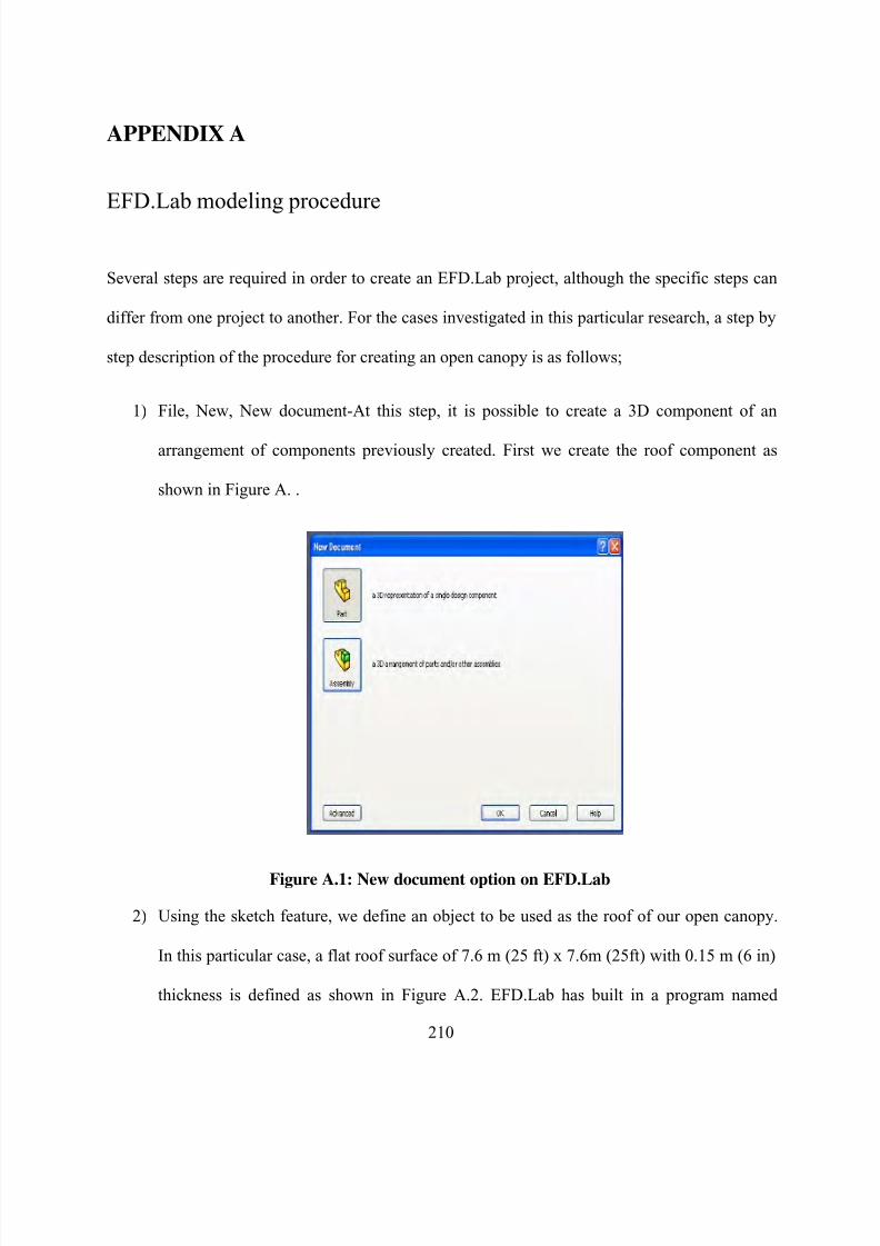
8/22/2019 Open Canopy Wind With Parapets
http://slidepdf.com/reader/full/open-canopy-wind-with-parapets 234/275
210
APPENDIX A
EFD.Lab modeling procedure
Several steps are required in order to create an EFD.Lab project, although the specific steps can
differ from one project to another. For the cases investigated in this particular research, a step by
step description of the procedure for creating an open canopy is as follows;
1) File, New, New document-At this step, it is possible to create a 3D component of an
arrangement of components previously created. First we create the roof component as
shown in Figure A. .
Figure A.1: New document option on EFD.Lab
2) Using the sketch feature, we define an object to be used as the roof of our open canopy.
In this particular case, a flat roof surface of 7.6 m (25 ft) x 7.6m (25ft) with 0.15 m (6 in)
thickness is defined as shown in Figure A.2. EFD.Lab has built in a program named

8/22/2019 Open Canopy Wind With Parapets
http://slidepdf.com/reader/full/open-canopy-wind-with-parapets 235/275
211
Solidworks (SolidWorks 2009). It is used in the program for creating 3D objects that can
have properties, like dimensions, thickness and materials, in order to create parts that can
be assembled later for the final CFD analysis.
Figure A.2: Roof surface created using EFD.Lab
3) A new component, created with SolidWorks, to be used as the parapet of the open canopy
is modeled with the same dimensions of the roof surface. The thickness of the parapet
walls is 6 inches. Refer to Figure A.3.

8/22/2019 Open Canopy Wind With Parapets
http://slidepdf.com/reader/full/open-canopy-wind-with-parapets 236/275
212
Figure A.3: Parapet element created using EFD.Lab
4) A third component, called an assembly was created using the previously created single
parts, that combines the roof surface and the parapet created on the previous steps. This
final component to be used in the analysis is shown in Figure A.4.
Figure A.4: Canopy model combining roof element and parapet element using EFD.Lab
5) Using the wizard project configuration, the user should specify the Units to used in the
analysis, the analysis type (choosing between internal and external flow), default fluid to
be used (in this case air), wall conditions, and initial and ambient conditions. With

8/22/2019 Open Canopy Wind With Parapets
http://slidepdf.com/reader/full/open-canopy-wind-with-parapets 237/275
213
reference to Figure A.5 through Figure A.8, the parameters for pressure, temperature,
wind velocity and turbulence parameters can be included.
Figure A.5: EFD.Lab unit selection wizard screen.
Figure A.6: EFD.Lab screen for input of internal or external analysis.

8/22/2019 Open Canopy Wind With Parapets
http://slidepdf.com/reader/full/open-canopy-wind-with-parapets 238/275
214
Figure A.7: Fluid type and analysis type on EFD.Lab wizard.
Figure A.8: Initial and ambient conditions in EFD.Lab
6) Results and geometry resolution is the default option that the program uses to mesh the
domain. In this option, it is possible to specify the mesh density to be used in the
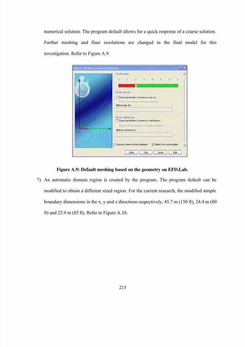
8/22/2019 Open Canopy Wind With Parapets
http://slidepdf.com/reader/full/open-canopy-wind-with-parapets 239/275
215
numerical solution. The program default allows for a quick response of a coarse solution.
Further meshing and finer resolutions are changed in the final model for this
investigation. Refer to Figure A.9.
Figure A.9: Default meshing based on the geometry on EFD.Lab.
7) An automatic domain region is created by the program. The program default can be
modified to obtain a different sized region. For the current research, the modified simple
boundary dimensions in the x, y and z directions respectively, 45.7 m (150 ft), 24.4 m (80
ft) and 25.9 m (85 ft). Refer to Figure A.10.

8/22/2019 Open Canopy Wind With Parapets
http://slidepdf.com/reader/full/open-canopy-wind-with-parapets 240/275
216
Figure A.10: Model and computational domain in EFD.Lab.
8) At this stage, the model is ready to be analyzed. The required time to solve the
mathematical model depends on the size of the domain and the meshing on the cells.
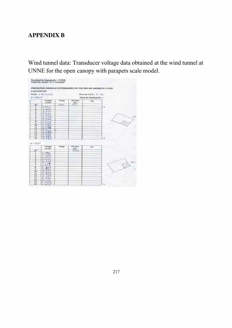
8/22/2019 Open Canopy Wind With Parapets
http://slidepdf.com/reader/full/open-canopy-wind-with-parapets 241/275
217
APPENDIX B
Wind tunnel data: Transducer voltage data obtained at the wind tunnel at
UNNE for the open canopy with parapets scale model.

8/22/2019 Open Canopy Wind With Parapets
http://slidepdf.com/reader/full/open-canopy-wind-with-parapets 242/275
218

8/22/2019 Open Canopy Wind With Parapets
http://slidepdf.com/reader/full/open-canopy-wind-with-parapets 243/275
219
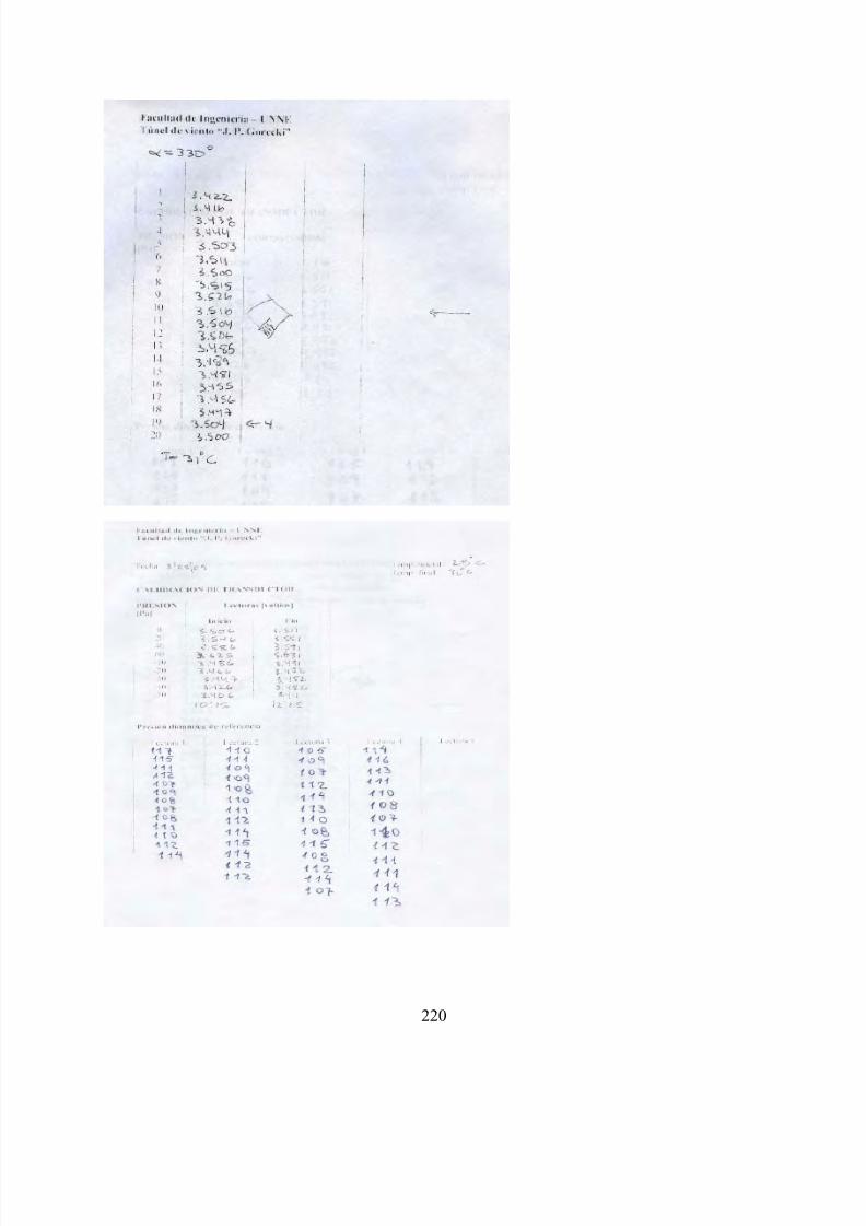
8/22/2019 Open Canopy Wind With Parapets
http://slidepdf.com/reader/full/open-canopy-wind-with-parapets 244/275
220

8/22/2019 Open Canopy Wind With Parapets
http://slidepdf.com/reader/full/open-canopy-wind-with-parapets 245/275
221

8/22/2019 Open Canopy Wind With Parapets
http://slidepdf.com/reader/full/open-canopy-wind-with-parapets 246/275
222
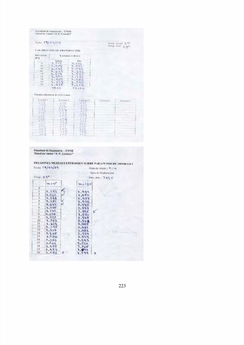
8/22/2019 Open Canopy Wind With Parapets
http://slidepdf.com/reader/full/open-canopy-wind-with-parapets 247/275
223

8/22/2019 Open Canopy Wind With Parapets
http://slidepdf.com/reader/full/open-canopy-wind-with-parapets 248/275
224
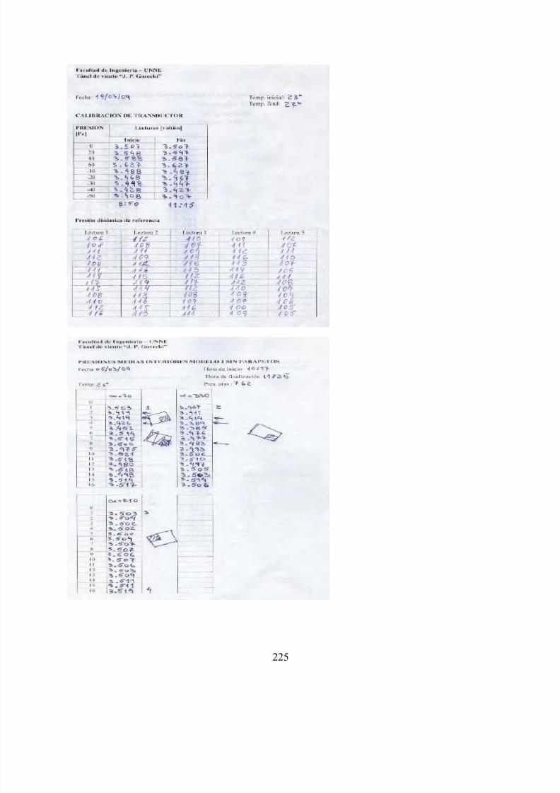
8/22/2019 Open Canopy Wind With Parapets
http://slidepdf.com/reader/full/open-canopy-wind-with-parapets 249/275
225

8/22/2019 Open Canopy Wind With Parapets
http://slidepdf.com/reader/full/open-canopy-wind-with-parapets 250/275
226

8/22/2019 Open Canopy Wind With Parapets
http://slidepdf.com/reader/full/open-canopy-wind-with-parapets 251/275
227
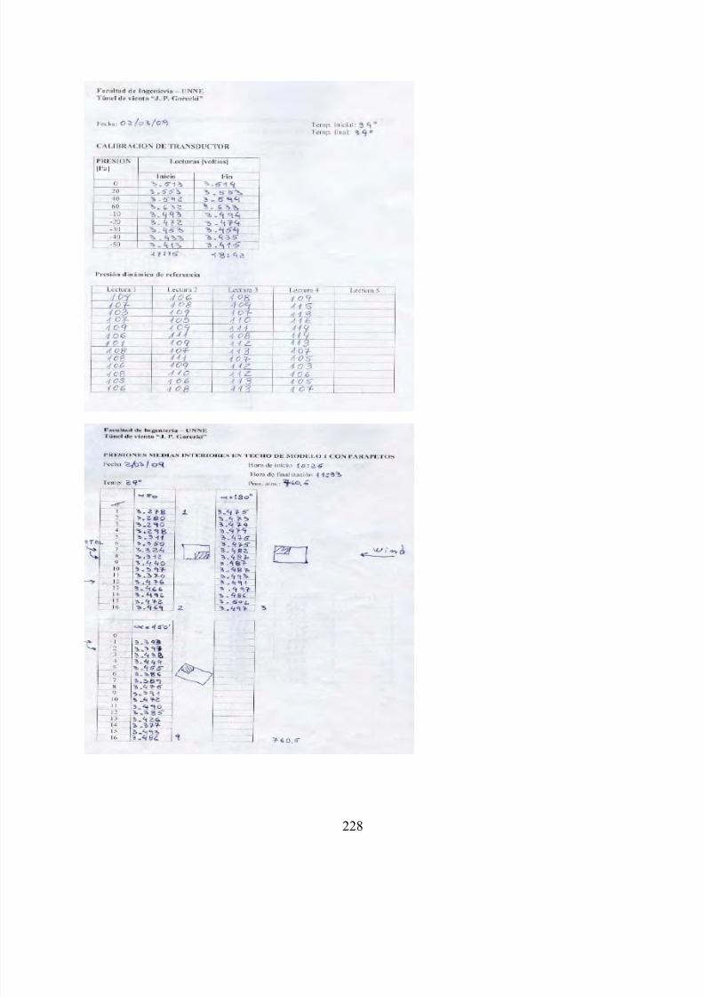
8/22/2019 Open Canopy Wind With Parapets
http://slidepdf.com/reader/full/open-canopy-wind-with-parapets 252/275
228
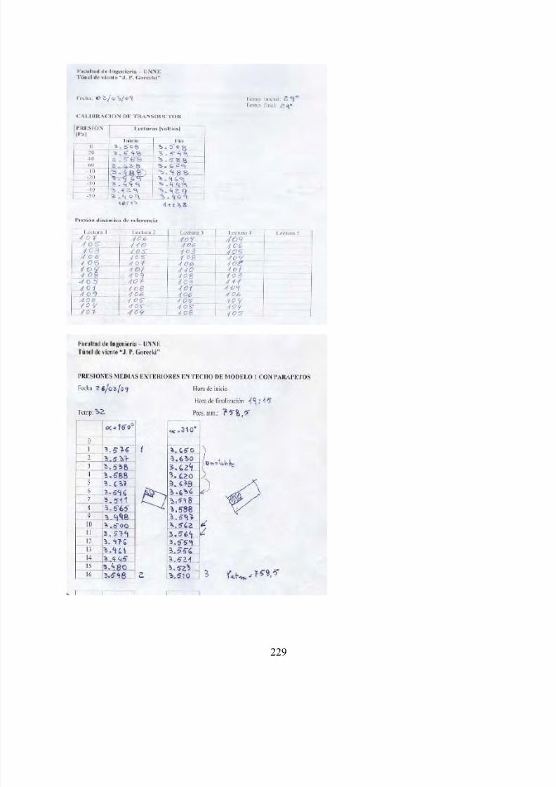
8/22/2019 Open Canopy Wind With Parapets
http://slidepdf.com/reader/full/open-canopy-wind-with-parapets 253/275
229

8/22/2019 Open Canopy Wind With Parapets
http://slidepdf.com/reader/full/open-canopy-wind-with-parapets 254/275
230

8/22/2019 Open Canopy Wind With Parapets
http://slidepdf.com/reader/full/open-canopy-wind-with-parapets 255/275
231

8/22/2019 Open Canopy Wind With Parapets
http://slidepdf.com/reader/full/open-canopy-wind-with-parapets 256/275
232

8/22/2019 Open Canopy Wind With Parapets
http://slidepdf.com/reader/full/open-canopy-wind-with-parapets 257/275
233

8/22/2019 Open Canopy Wind With Parapets
http://slidepdf.com/reader/full/open-canopy-wind-with-parapets 258/275
234
APPENDIX C
Open canopy without parapets: spreadsheet calculations.

8/22/2019 Open Canopy Wind With Parapets
http://slidepdf.com/reader/full/open-canopy-wind-with-parapets 259/275
235

8/22/2019 Open Canopy Wind With Parapets
http://slidepdf.com/reader/full/open-canopy-wind-with-parapets 260/275
236

8/22/2019 Open Canopy Wind With Parapets
http://slidepdf.com/reader/full/open-canopy-wind-with-parapets 261/275
237

8/22/2019 Open Canopy Wind With Parapets
http://slidepdf.com/reader/full/open-canopy-wind-with-parapets 262/275
238
APPENDIX D
Open canopy with parapets: spreadsheet calculations.
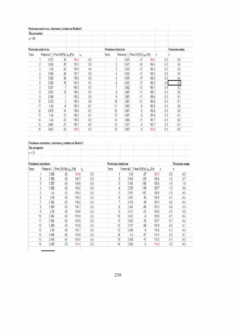
8/22/2019 Open Canopy Wind With Parapets
http://slidepdf.com/reader/full/open-canopy-wind-with-parapets 263/275
239

8/22/2019 Open Canopy Wind With Parapets
http://slidepdf.com/reader/full/open-canopy-wind-with-parapets 264/275
240

8/22/2019 Open Canopy Wind With Parapets
http://slidepdf.com/reader/full/open-canopy-wind-with-parapets 265/275
241

8/22/2019 Open Canopy Wind With Parapets
http://slidepdf.com/reader/full/open-canopy-wind-with-parapets 266/275
242
APPENDIX E
Parapets: spreadsheet calculations.
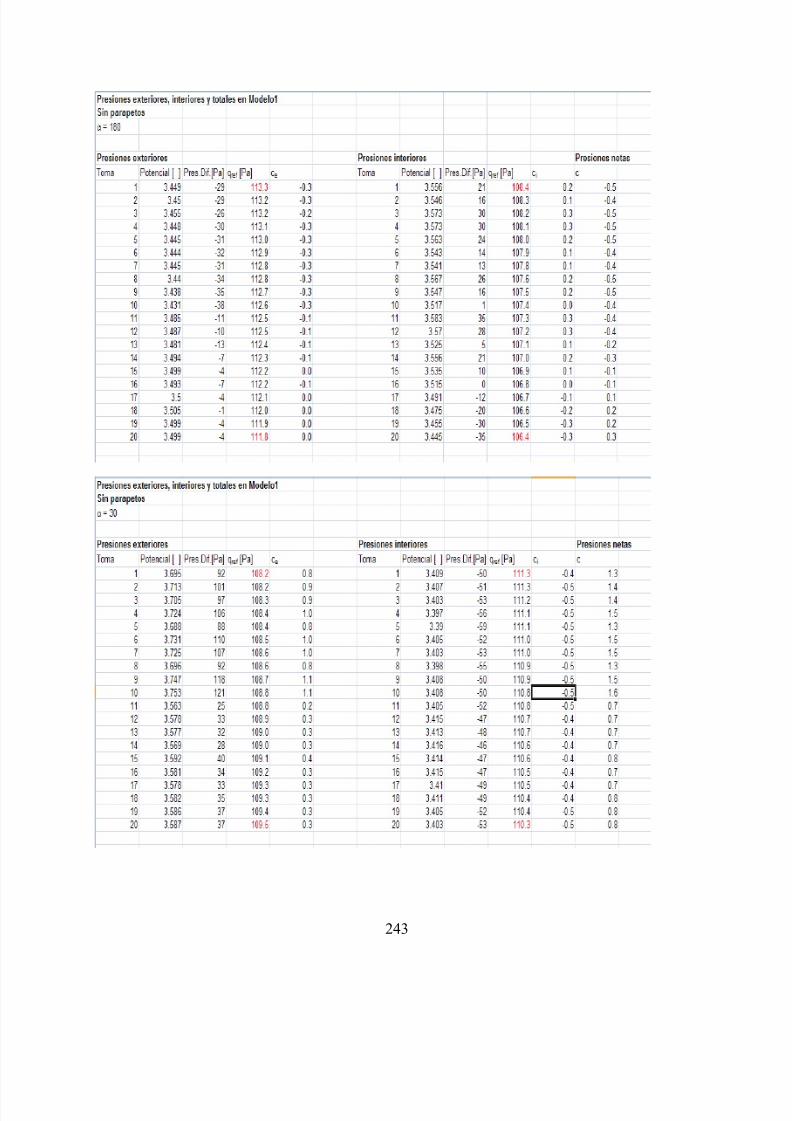
8/22/2019 Open Canopy Wind With Parapets
http://slidepdf.com/reader/full/open-canopy-wind-with-parapets 267/275
243

8/22/2019 Open Canopy Wind With Parapets
http://slidepdf.com/reader/full/open-canopy-wind-with-parapets 268/275
244
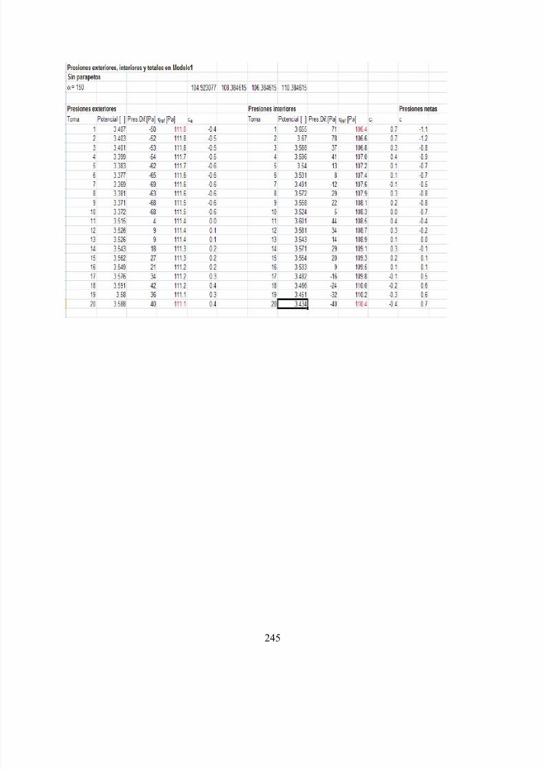
8/22/2019 Open Canopy Wind With Parapets
http://slidepdf.com/reader/full/open-canopy-wind-with-parapets 269/275
245

8/22/2019 Open Canopy Wind With Parapets
http://slidepdf.com/reader/full/open-canopy-wind-with-parapets 270/275
246
APPENDIX F
CFD test of different wind angles on open canopy to verify assumption
of wind at 0° and 30°.
Wind at 0°.
Wind at 15°.

8/22/2019 Open Canopy Wind With Parapets
http://slidepdf.com/reader/full/open-canopy-wind-with-parapets 271/275
247
Wind at 30°.
Wind at 45°.

8/22/2019 Open Canopy Wind With Parapets
http://slidepdf.com/reader/full/open-canopy-wind-with-parapets 272/275
248
Wind at 60°.
Wind at 75°.
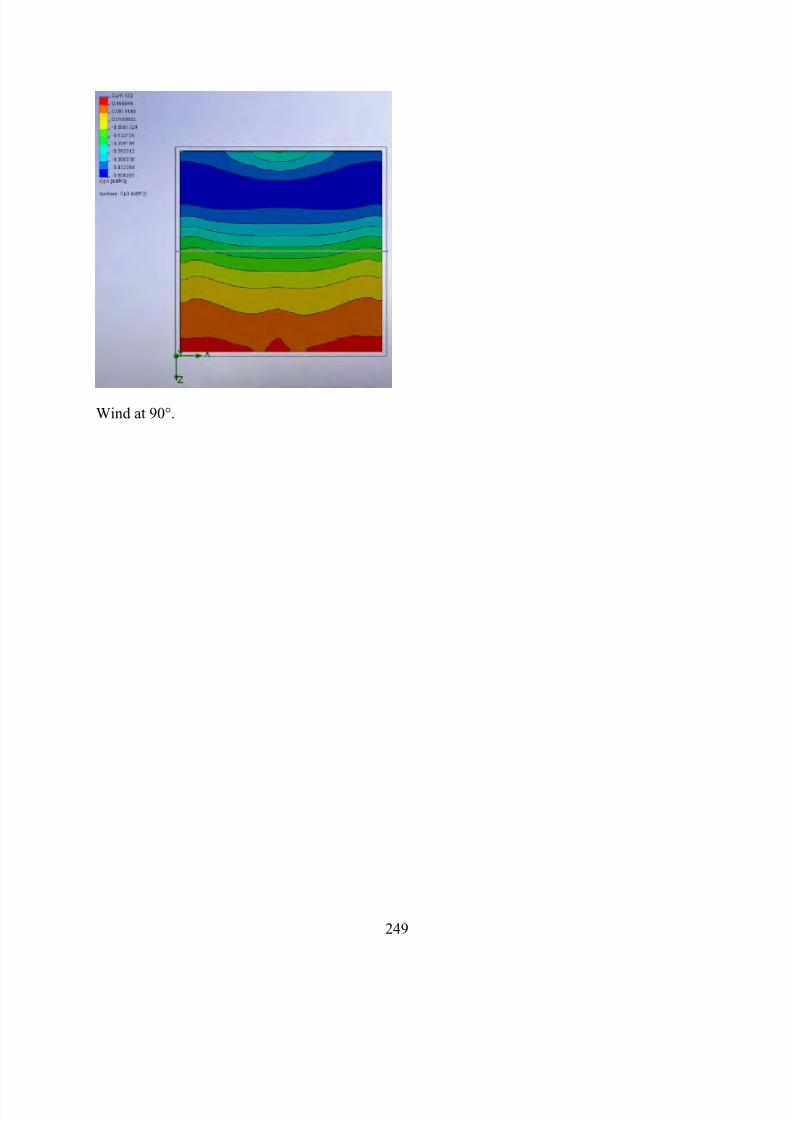
8/22/2019 Open Canopy Wind With Parapets
http://slidepdf.com/reader/full/open-canopy-wind-with-parapets 273/275
249
Wind at 90°.
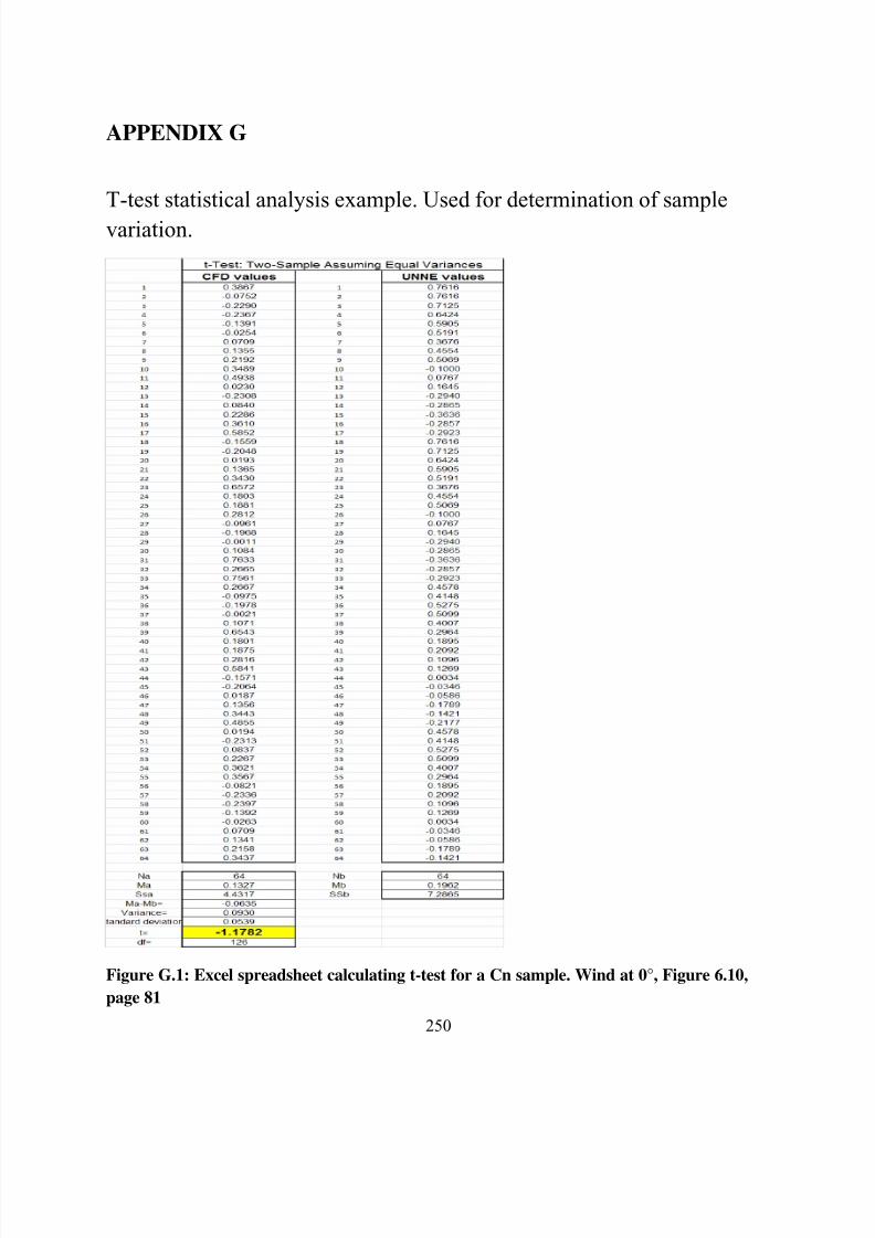
8/22/2019 Open Canopy Wind With Parapets
http://slidepdf.com/reader/full/open-canopy-wind-with-parapets 274/275
250
APPENDIX G
T-test statistical analysis example. Used for determination of sample
variation.
Figure G.1: Excel spreadsheet calculating t-test for a Cn sample. Wind at 0°, Figure 6.10,
page 81

8/22/2019 Open Canopy Wind With Parapets
http://slidepdf.com/reader/full/open-canopy-wind-with-parapets 275/275