LES MODELING OF CANOPY FLOWS FORLES MODELING OF CANOPY FLOWS FOR WIND PREDICTION IN URBAN AREA

Zhenqing LiuTakeshi IshiharaTakeshi Ishihara

Bridge & Structure LabBridge & Structure LabDepartment of Civil Engineering

University of Tokyo

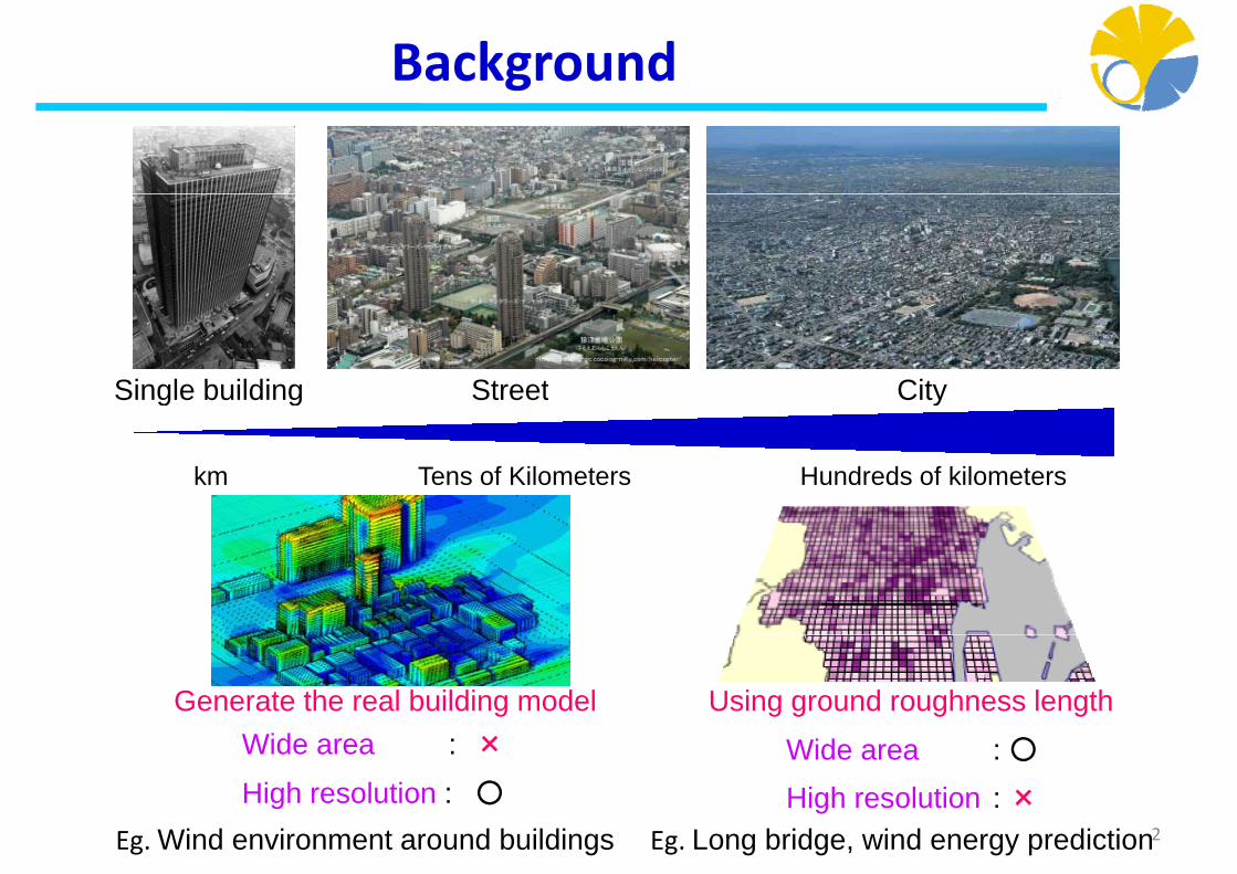
Background

Single building Street CitySingle building Street City

km Tens of Kilometers Hundreds of kilometers

Using ground roughness lengthGenerate the real building modelWide area : × Wide area : ○High resolution : ○ High resolution : ×

Eg. Wind environment around buildings Eg. Long bridge, wind energy prediction2

Objectives

• Propose a method to simulated the flow over urban area• Propose a method to simulated the flow over urban area• Validate the method by comparing the simulated results with

experimentsexperiments.• Check if the method could give good results for Two different

t f i t i b i b ildi d f ttypes of canopy exists in urban area, i.e. buildings and forest.

3

Fundamental equation

Continuity equation¶ 0i

i

ux¶ =¶

Momentum equation

i j iji iu uu u p tæ ö¶ ¶¶ ¶ ¶ ¶÷ç ÷ In fluid

In roughness

i j iji i

j j j i j

u u pt x x x x x

r r m¶ ¶¶ ¶ ¶ ¶÷ç ÷+ = ç - -÷ç ÷÷ç¶ ¶ ¶ ¶ ¶ ¶è ø

i j iju uu u p tæ ö¶ ¶¶ ¶ ¶ ¶÷ç In roughness canopy ,

i j iji iu i

j j j i j

u uu u p ft x x x x x

tr r m

æ ö¶ ¶¶ ¶ ¶ ¶÷ç ÷+ = ç - - +÷ç ÷÷ç¶ ¶ ¶ ¶ ¶ ¶è ø

Smagorinsky‐Lilly SGS model1 12 ; ji

ij t ij kk ij ijuuS St m t d

æ ö¶¶ ÷ç ÷= - + = ç + ÷

Cs=0.032

2 ;3 2

ij t ij kk ij ijj i

S Sx x

t m t d= - + = ç + ÷ç ÷÷ç¶ ¶è ø1

2 32 ; min ,t s s ij ij s sL S L S S L d C Vm r r kæ ö÷ç ÷= = = ç ÷ç ÷çè ø

s÷çè ø

4

Flow pattern V.S. density of roughness

Ishihara et al. (1997)

Isolated roughness flow

W k i t f flWake interference flowFrontal density<10%

Ski i flSkimming flow (cavity flow）

Frontal density>30% 5

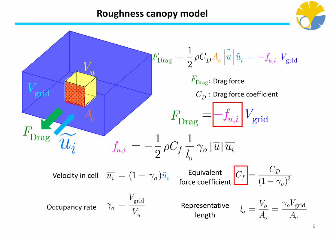
Roughness canopy model

1 A g drag r, iD

12 ioD u iuA u VfF Cr -==

D fuV

F

gridV:

:

Drag force

Drag force coefficient

DragF

DC

DragF rid, gu i Vf-=oA

F iu ,1 12 f o ii

ou Cf u u

lr g= -

DragF

ol

(1 )i io uu g= - 2(1 )D

fo

CCg

=-

Velocity in cell Equivalent force coefficient ( )og

gridoo VVlg

= =grid

o

V

Vg =Occupancy rate 

force coefficient

Representative o

o ol

A AuVp y

length6

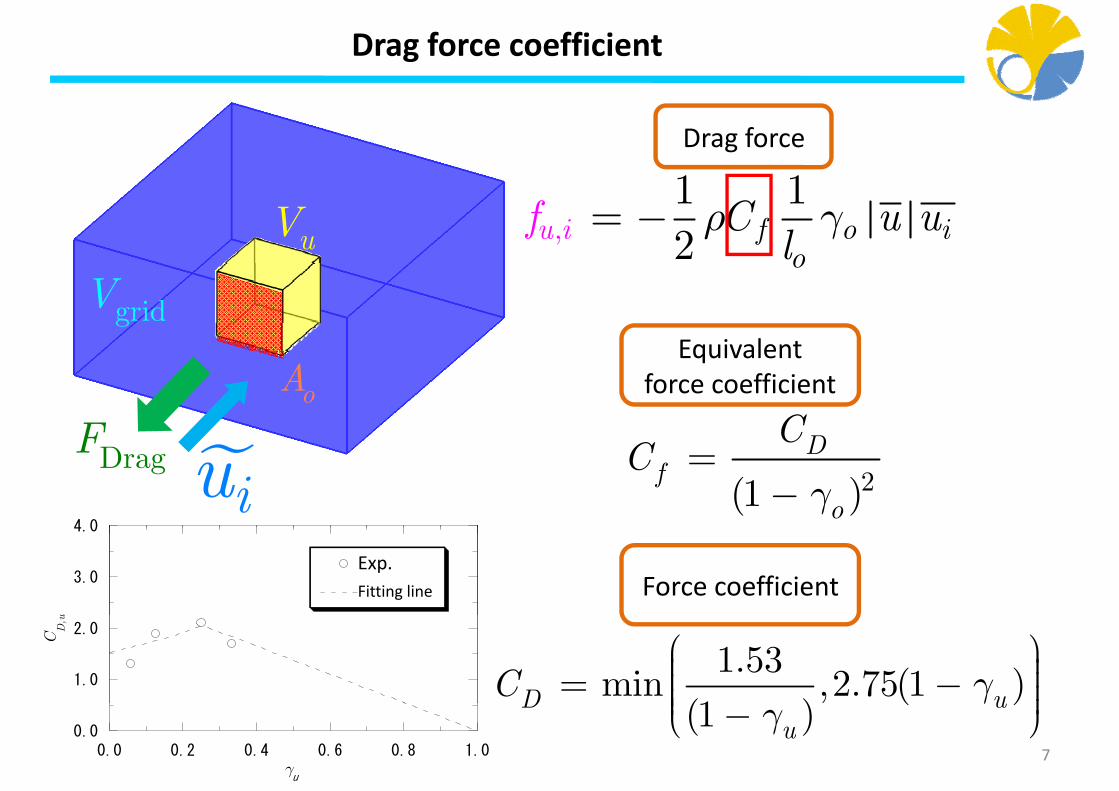
Drag force coefficient

1 1Drag force

,1 12 f o ii

ou Cf u u

lr g= -uV o

gridVEquivalent

DCoA

F

Equivalent force coefficient

4 0

2(1 )D

fo

CC

g=

-iuDragF

3.0

4.0

風洞実験

式

u

Force coefficientExp.Fitting line

1.0

2.0CD,u

1.53min ,2.75(1 )(1 )D uC gæ ö÷ç ÷= -ç ÷ç ÷ç

0.00.0 0.2 0.4 0.6 0.8 1.0

gu

, ( )(1 )D u

u

ggç ÷ç -è ø

7

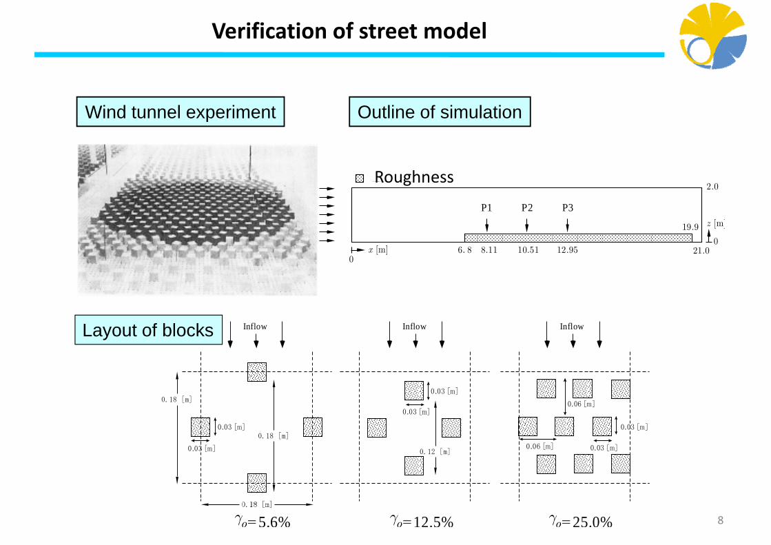
Verification of street model

Outline of simulationWind tunnel experimentp

粗度ブロックRoughness2.0

0

z [m]

粗度 ック

P1

19.9

P2 P3

Roughness

x [m]0

21.00

6.8

Case0

8.11 10.51 12.95

Layout of blocks InflowInflowInflow

0.18 [m]

[ ]

0.06 [m]0.03 [m]

0.03 [m]

[ ]

0.03 [m]

0.03 [m]

0.06 [m]0.12 [m]

0.18 [m]

0.03 [m]

0.03 [m]

8go=5.6% go=12.5% go=25.0%

Numerical model

XY

Z

2OutletBird’s view Side view

2

X

z

1

2Outlet

x1015

20

1

z

0

1

x0 5 10 15 200

Roughness Canopy

x

05y 0

0.51

Inflow velocity Profile0 5

Inlet

0.3

0.4

0.5

m) Growing rate: 1.1 Horizontal resolution: h

Roughness Canopy0

0.1

0.2

z(m

10 gridsCanopy top grid size: 0.002m

g Horizontal resolution: h

h g py0.2 0.4 0.6 0.8 1 1.2

0

u(m/s)

gFirst grid size: 0.002m

9

Instantaneous flow fields over modeled roughness canopy

Occupancy 5.6%

Instantaneous flow fields visualized by vorticity

Occupancy 5.6%

Horizontal Slice z=1h

Hori ontal Slice 2hHorizontal Slice z=2h

Occupancy 12.5%

Horizontal Slice z=1h

Horizontal Slice z=2h

Occupancy 25.0%

Horizontal Slice z=1hHorizontal Slice z=1h

Horizontal Slice z=2h

Instantaneous turbulent flow fields are successfully captured 10

Comparison with experiments

Occupancy 5 6%

1m s‐1 0.025m2 s‐2SimulationExperiment

SimulationExperiment

Mean Wind Speed Turbulent Kinetic Energy5.6%

Occupancy p y12.5%

Occupancy 25.0%

Mean wind speed and kinetic energy are well reproduced. 11

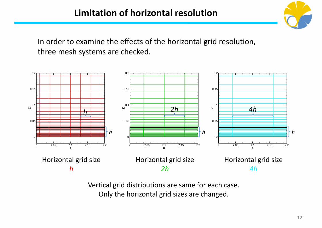
Limitation of horizontal resolution

In order to examine the effects of the horizontal grid resolution, three mesh systems are checkedthree mesh systems are checked.

h 2h 4h

h h h

Horizontal grid size h

Horizontal grid size 2h

Horizontal grid size 4h

Vertical grid distributions are same for each case.Only the horizontal grid sizes are changed.

12

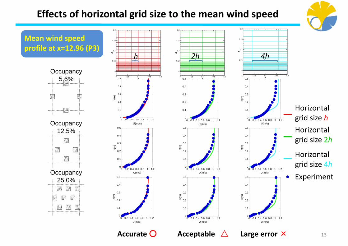
Effects of horizontal grid size to the mean wind speed

Mean wind speed profile at x=12.96 (P3)

2h 4hh

Occupancy 5.6% 0.5 0.5 0.5

2h 4hh

0 1

0.2

0.3

0.4

h(m

)0 1

0.2

0.3

0.4

0 1

0.2

0.3

0.4

h(m

)

Horizontal

Occupancy 12.5%

0 0.2 0.4 0.6 0.8 1 1.20

0.1

U(m/s)0 0.2 0.4 0.6 0.8 1 1.2

0

0.1

U(m/s)0 0.2 0.4 0.6 0.8 1 1.2

0

0.1

U(m/s)

0.4

0.5

0.4

0.5

0.4

0.5

Horizontal grid size hHorizontal 

h

0.1

0.2

0.3

h(m

)

0.1

0.2

0.3

h(m

)

0.1

0.2

0.3

h(m

)

grid size 2h

Horizontal grid size 4h

Occupancy 25.0%

0 0.2 0.4 0.6 0.8 1 1.20

U(m/s)0 0.2 0.4 0.6 0.8 1 1.2

0

U(m/s)0 0.2 0.4 0.6 0.8 1 1.2

0

U(m/s)

0.4

0.5

0.4

0.5

0.4

0.5 Experimentgrid size 4h

0 0.2 0.4 0.6 0.8 1 1.20

0.1

0.2

0.3

h(m

)

0 0 2 0 4 0 6 0 8 1 1 20

0.1

0.2

0.3

h(m

)

0 0 2 0 4 0 6 0 8 1 1 20

0.1

0.2

0.3

h(m

)

0 0.2 0.4 0.6 0.8 1 1.2U(m/s)

0 0.2 0.4 0.6 0.8 1 1.2U(m/s)

0 0.2 0.4 0.6 0.8 1 1.2U(m/s)

Accurate ○ Acceptable △ Large error × 13

Effects of horizontal grid size to the kinetic energy

Kinetic energy profile at x=12.96 (P3)

2h 4hh

0.5 0.5 0.5

Occupancy 5.6%

2h 4hh

0 1

0.2

0.3

0.4

h(m

)

0 1

0.2

0.3

0.4

h(m

)

0 1

0.2

0.3

0.4

h(m

)

Horizontal0 0.005 0.01 0.015 0.02

0

0.1

k(m2/s2)

0.4

0.5

0 0.005 0.01 0.015 0.020

0.1

k(m2/s2)

0.4

0.5

0 0.005 0.01 0.015 0.020

0.1

k(m2/s2)

0.4

0.5Occupancy

12.5%

Horizontal grid size hHorizontal 

h

0.1

0.2

0.3

0.4

h(m

)

0.1

0.2

0.3

0.4

h(m

)

0.1

0.2

0.3

0.4

h(m

)

grid size 2h

Horizontal grid size 4h

0 0.005 0.01 0.015 0.02 0.0250

k(m2/s2)

0.4

0.5

0 0.0050.01 0.0150.02 0.0250

k(m2/s2)

0.4

0.5

0 0.005 0.01 0.015 0.02 0.0250

k(m2/s2)

0.4

0.5Occupancy

25.0% Experimentgrid size 4h

0 0 005 0 01 0 015 0 020

0.1

0.2

0.3

h(m

)

0 0 005 0 01 0 015 0 020

0.1

0.2

0.3

h(m

)

0 0 005 0 01 0 015 0 020

0.1

0.2

0.3

h(m

)

0 0.005 0.01 0.015 0.02k(m2/s2)

0 0.005 0.01 0.015 0.02k(m2/s2)

0 0.005 0.01 0.015 0.02k(m2/s2)

Accurate ○ Acceptable △ Large error × 14

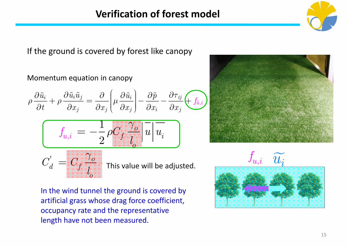
Verification of forest model

If the ground is covered by forest like canopyg y py

Momentum equation in canopy

,i j iji i

u ij j j i j

u uu u pt x x x

fx x

tr r m

æ ö¶ ¶¶ ¶ ¶ ¶÷ç ÷+ = ç - - +÷ç ÷÷ç¶ ¶ ¶ ¶ ¶ ¶è ø

j j j i jt x x xx x¶ ¶ ¶ ¶ ¶ ¶è ø

12

of iu i Cf u ulg

r= -, 2 f io

u if lr

iu,u if' od fC C

g= Thi l ill b dj t d i,

In the wind tunnel the ground is covered by

d fo

C Cl

= This value will be adjusted.

In the wind tunnel the ground is covered by artificial grass whose drag force coefficient, occupancy rate and the representative l th h t b dlength have not been measured.  

15

Numerical model

Grid No. 7.5million

10mm

,1 12 f o iiu Cf u u

lr g= -

Roughness canopy

2 ol

10m

m' 8.0od f

o

C Clg

= =

MeanMean wind speed Fluctuations

σi/Uref

Simulated results for the flow fields over forest are accurate. 16

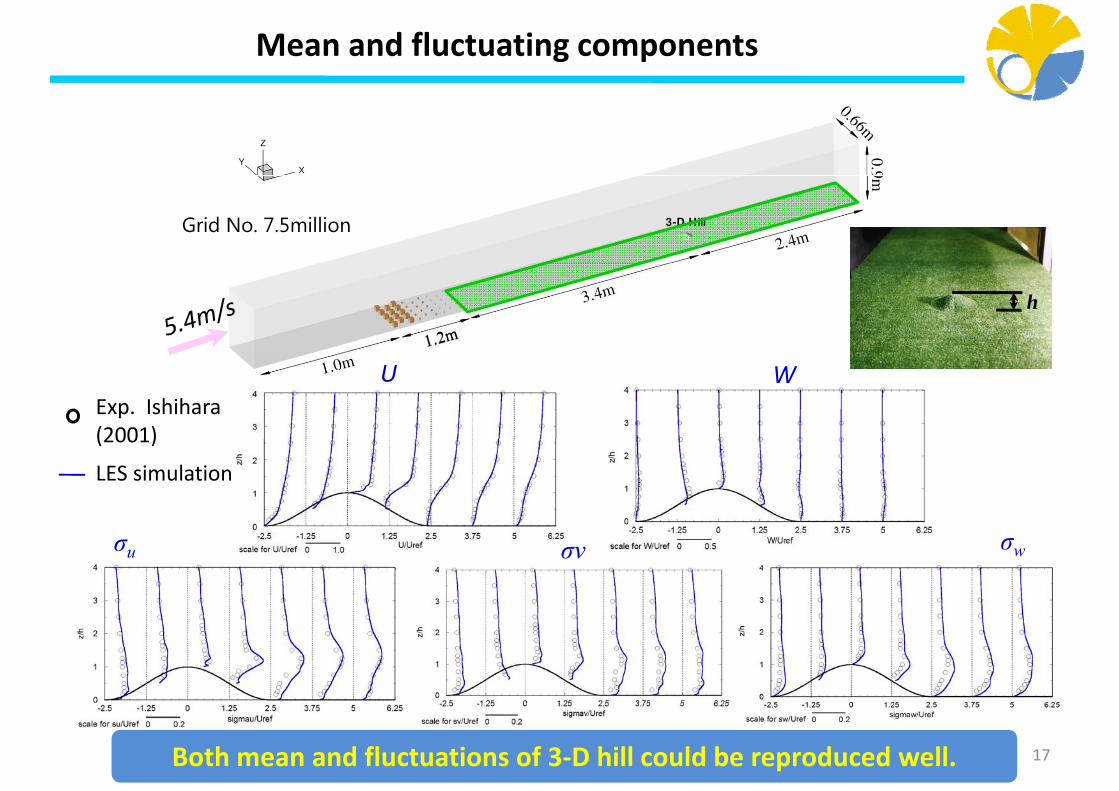
Mean and fluctuating components

Grid No. 7.5million

h

U WExp.  Ishihara (2001)(2001)

LES simulation

σu σv σw

Both mean and fluctuations of 3‐D hill could be reproduced well. 17

Conclusions

• A method simulating the roughness canopy by adding asource term in the momentum equation are proposed.

• The flow fields over the roughness blocks are successfullyreproduced by using this method. Simulated results showgood agreement with experiment.

• The same method are applied for the flow over the artificialppgrass, and with adjusting the equivalent force coefficients theflow fields are well reproduced.

18

Thanks for your attention!