The Interdisciplinary Center Herzliya

Efi Arazi School of Computer Science

Online Classification of VoD and Live Video Streaming Applications

M.Sc. Dissertation

Submitted in Partial Fulfillment of the Requirements for the

Degree of Master of Science (M.Sc.) Research Track

in Computer Science

Submitted by Shuval Polacheck

Under the supervision of Dr. Ronit Nossenson

June 2013

2

Acknowledgements

I would like to express my gratitude to a number of people who made crucial contributions to

this work. First of all, I would like to thank my advisor, Dr. Ronit Nossenson, whose expert

guidance and constant encouragement made possible the pursuit and completion of this work. I

would also like to thank Prof. Tami Tamir, who supervised my work on behalf of the IDC and

provided important and helpful comments. Finally, I would like to thank Elad Hefetz from Bezeq

International, for providing us with the data set we relied on in this work.

3

Abstract

Streaming media services deliver audio and video without making the viewer wait to download

the file. As the user plays the media file, the service continues to download and buffer additional

content from the streaming server. Multimedia streaming can be divided into two categories:

Video on Demand (VoD), where all frames are available at all times; and Live, where only the

last frames are available. Different solutions have been proposed to optimize both Live streaming

(e.g., multicast) and VoD (e.g., Cache, Streaming Peer-to-Peer). Implementation of these

solutions in an Internet Service Provider (ISP) network requires an online classification

capability between Live and VoD streams. In this work, we propose and evaluate two approaches

for the online classification problem: a statistical approach based on packet length; and a flow

comparison approach based on information offset of two different streaming flows. We defined

information offset as the difference between the arrival times of identical packets in two different

flows. To evaluate our classifiers, we used a dataset collected for this research by the Israeli ISP

Bezeq International. We use 20% of the pre-tagged dataset for offline learning and the other 80%

to evaluate our classifiers. Our statistical classifier tags 96% of the streams correctly, while our

comparative classifier successfully tags 96.5% of streams. We also demonstrate a more complex

multi-streaming comparing function that improves the success rate of our algorithm to 97.53%.

We note that while the comparative classifier clearly achieves better classification results, the

statistical classifier, is easier to implement, as it does not require an additional stream to compare

with.

4

Table of Contents

I. Introduction ........................................................................................................................................................ 5

II. Related Work ...................................................................................................................................................... 9

III. Main Contributions of this Work .................................................................................................................... 11

IV. Dataset Collection ............................................................................................................................................. 12

V. Statistical Characterization ............................................................................................................................. 13

(1) Statistical Characterization of Live Video Streaming Traffic......................................................................... 13

(2) Statistical Characterization of VoD Streaming Traffic .................................................................................. 13

VI. Video Streaming Application Classifiers ........................................................................................................ 16

(1) Statistical Classifier ....................................................................................................................................... 17

(2) Comparative Classifier ................................................................................................................................... 20

VII. Performance Evaluation .................................................................................................................................. 25

(1) Statistical Classifiers Performance ................................................................................................................ 25

(2) Comparative Classifiers Performance ........................................................................................................... 26

Table 5. The single pair classifier results ................................................................................................................. 26

VIII. Conclusions ....................................................................................................................................................... 28

IX. References ......................................................................................................................................................... 29

5

I. Introduction

According to Cisco Visual Networking Index (VNI) 2011-2016 [1], internet video will drive most

consumer Internet traffic through 2016. The sum of all forms of IP video (Internet video, IP VoD,

video files exchanged through file sharing, video streamed gaming, and videoconferencing) will

ultimately reach 86% of total IP traffic. Taking a more narrow definition of Internet video that

excludes file sharing and gaming, Internet video will account for 55% of consumer Internet traffic

in 2016 (see Figure 1). Internet video officially reached the halfway mark of consumer Internet

traffic by the end of 2012.

The implications of video growth are difficult to overstate. With video growth, Internet traffic is

evolving from a relatively steady stream of traffic to a more dynamic traffic pattern. Because

video has a higher peak-to-average ratio than data or file sharing, and because video is gaining

traffic share, peak Internet traffic will grow faster than average traffic. With video, the Internet

now has a much busier busy hour. The growing gap between peak and average traffic is amplified

further by the changing composition of Internet video. As shown in Figure 2 and Table 1, real-

time video such as live video, ambient video, and video calling, are taking an ever greater share of

video traffic [1]. Real-time video has a peak-to-average ratio that is higher than on-demand video.

Streaming media services (e.g., Live video streaming and Video on Demand, or VoD, streaming)

deliver audio and video without making the viewer wait to download files. As the user plays the

media file, the service continues to download and buffer additional content from the streaming

server. Playing and downloading happen at the same time. Delivering video streaming services

over a best-effort packet network, such as the Internet, is complicated by a number of factors,

including unknown and time-varying bandwidth, delay, and losses, as well as many additional

issues, such as how to fairly share the network resources amongst many flows, and how to

efficiently perform one-to-many communications for popular content. Thus, streaming video

over the Internet has received tremendous attention from academia and industry. Different

solutions have been proposed for Live video streaming (e.g., multicast technologies) and for

VoD streaming (e.g., Video Cache technologies, Streaming Peer-to-Peer technologies).

However, to implement these solutions in an Internet service provider (ISP) network, an online

classification of video streaming flows (or video streaming sources) into a Live streaming class

and a VoD streaming class is required. This classification should be performed as soon as

possible to allow proper flow optimization.

Commonly deployed IP traffic classification techniques have been based on direct inspection of

each packet’s contents at some point on the network. Successive IP packets having the same 5-

tuple of protocol type, source address, source port, destination address, and destination port are

considered to belong to a flow whose controlling application we wish to determine. Simple

classification infers the controlling application’s identity by assuming that most applications

consistently use ‘well known’ TCP or UDP port numbers (visible in the TCP or UDP headers).

However, many applications are increasingly using unpredictable (or at least obscure) port

numbers [2]. Consequently, more sophisticated classification techniques infer application type by

looking for application-specific data (or well-known protocol behavior) within the TCP or UDP

payloads [2, 3].

6

Figure 1. Global consumer Internet traffic [1]

Figure 2. Global consumer Internet video traffic [1]

7

Video

Category Usage in 2011 Definition

Short form 12%

User-generated video and other video

clips generally less than 7 minutes in

length

Video calling 3.5% Video messages/calling

Long form 61% Video content generally greater than 7

minutes in length

Internet video to

TV 8%

Video delivered through the Internet to a

TV screen

Live internet TV 9%

Peer-to-peer TV (excluding P2P video

downloads) and live television streaming

over the Internet

Internet PVR 1% Recording live TV content

Ambient video 2.5% Nannycams, petcams, home security

cams, and other persistent video streams

Mobile video 3% All video that travels over a 2G, 3G, or

4G network

Table 1. Global consumer Internet video traffic, 2011-2016 [1]

The research community has responded by investigating classification schemes capable of

inferring application-level usage patterns without deep packet inspection (DPI). Newer

approaches classify traffic by recognizing statistical patterns in externally observable attributes of

the traffic (such as typical packet lengths and inter-packet arrival times). Their ultimate goal is

either clustering IP traffic flows into groups that have similar traffic patterns, or classifying one or

more applications of interest, as discussed below. However, none of the previous research has

solved the problem of statistical streaming application classification into live streaming type and

VoD streaming type. Since these two applications use the same streaming protocols, DPI

technologies are practically useless in solving this problem.

In our work we examined and evaluated two types of online streaming application classifiers.

First, we reviewed and developed a statistical approach for a streaming application classifier. This

statistical online streaming classifier entails the classification of traffic according to statistical

patterns in externally observable attributes of the traffic; in particular, it analyzes the measured

statistical differences between packet length distribution of VoD streaming applications and Live

video streaming applications. We then took a different approach, developing a comparative

classifier based on the simple observation that live streaming flows from the same video

streaming source transfer the same information almost at the same time, while VoD flows from

the same video streaming source have larger information offset. In light of this, the second

classifier analyzes and compares the data content of different flows from the same video

streaming source during a small time interval. This analysis allows us to distinguish whether these

flows are live video streaming flows or VoD streaming flows. Clearly, this online classifier

8

requires more than one flow from the same video streaming source, as it cannot classify a single

flow. It is important to mention that both classifiers are unable to analyze encrypted flows since

they are based on the packet’s raw data and packet length, which are unpredictable under

encryption.

Evaluation of the classifiers’ performance is based on real trace collected for this research by

Bezeq International, a large Israeli Internet service provider [4]. The trace includes captures of

one hour of streaming flows of live and VoD servers located at Bezeq International’s datacenter.

In the performance analysis, the flows are pre-tagged as live or VoD, but these tags are not

provided for the online classifiers. To evaluate the classifiers’ accuracy, the results of the online

classifier tags and the actual tags are compared. We used 20% of the trace data to optimize the

algorithm parameters (i.e, to build the classification off-line models) and the other 80% of the

trace was used to evaluate the algorithms’ performance. The statistical classifier correctly tagged

96% of the trace video streaming flows, while the comparative classifier correctly tagged 96.5%

of the trace video streaming flows. We demonstrated that adding more flow pairs to the algorithm

input can increase the tagging accuracy but it clearly decreases the algorithm scalability.

This work is structured as follows: In Chapter II, we list related work in internet application

classification. In Chapter III, we address the main contributions of this work to academia and

industry. Chapter IV describes the data collected for this work. In Chapter V, we review the

statistical characterization of our dataset. We then describe our two classification algorithms in

Chapter VI and their performances in Chapter VII. Finally, Chapter VIII reports our conclusions

and suggests possible directions for future research.

9

II. Related Work

Classifying traffic into specific network applications is essential for application-aware network

management. While port number-based classifiers work only for some well-known applications,

and signature-based classifiers are not applicable to encrypted packet payloads, researchers have

suggested classifying network traffic based on statistical behaviors observed in network

applications. Such methods assume that the statistical properties of traffic are unique for different

applications and can be used to distinguish between applications. Below we describe the state-of-

the-art of the statistical-based application classification.

The commonly used statistical features in statistical-based application classification are flow

duration, packet inter-arrival time, packet size, bytes transferred, number of packets, etc. Earlier

work just focused on the characteristics of network traffic classes or applications. Paxson [5]

studied the relationship between statistical properties of flows and applications that generate

them based on Internet traffic characterization. Paxson [5] and Paxson and Floyd [6] modeled

and analyzed the individual connection characteristics, such as bytes transferred, duration, inter-

arrival times and periodicity for different applications. Paxson and Floyd [6] found that arrivals

of user-initiated events, in applications such as TELNET or FTP control commands, can be

described by a Poisson process, whereas other applications arrivals deviate considerably from

Poisson. These works showed that it is possible to identify network traffic based on statistical

features.

Hereafter, more work endeavored to classify exclusively network traffic based on statistical

features. They generally consist of two parts: model building and classification. A model is first

built using statistical attributes of flows by learning the inherent structural patterns of datasets,

and the model is then used to classify other new unseen network traffic. Dewes et al. [7]

analyzed and classified different Internet chat traffic using multiple flow characteristics, such as

flow duration, packet inter-arrival time, packet size and bytes transferred. Roughan et al. [8] used

nearest neighbor (NN) and linear discriminate analysis (LDA) to map applications to a different

quality of service classes using features such as average packet size, flow duration, bytes per

flow, packet per flow and root mean square (RMS) packet size. Divakaran et al. [9] identified

different classes of applications by observing packet length and packet size of flow of a flow of

packets between two hosts in a network. Their approach is effective to classify short UDP flows,

such as DNS traffic. However, when applied to long-lasting flows or TCP flows, this approach

often makes incorrect decisions. Bernaille et al. [10] identified applications based on packet sizes

and directions of packets. Application behavior is clustered by characteristics observed in the

very first five packets of TCP connections. Subsequently, a flow is classified into an application

by measuring the minimum similarity distance. Ying-Dar et al. [11] used packet size distribution

(PSD) and packet size change cycle of a flow to model and classify application flows.

A few works analyze traffic at a level other than flow level. Kannan et al. [12] used a

connection-level trace to derive abstract descriptions of the session-structure for different

applications present in the trace. Based on the flows’ statistical information, Kannan’s approach

discovers and characterizes flow/session causality relationship. This approach can further infer

applications’ internal session structures. However, it may be not able to handle modern

sophisticated applications, since it identifies applications by using only port numbers.

Blind classification (BLINC), proposed by Karagiannis et al. [13], introduces another type of

approach for traffic classification based on the analysis of host behavior. It associates Internet

10

host behavior patterns with one or more applications, and refines the association by heuristics

and behavior stratification. It is able to accurately associate hosts with the service they provide or

use by inspecting all the flows generated by specific hosts.

Cellular backhaul networks carry user traffic within encrypted tunnels. With tunneled traffic, the

application classifier cannot identify the underlying TCP/UDP connections and cannot use any

IP packet header information. However, some statistical properties can be considered in this

case too, such as volume per tunnel, tunnel durations, inter-packets delays (however, sequential

packets might belong to different TCP connections), packet sizes and packet direction. In [14], a

blind online classification of the dominated application of user tunneled traffic is suggested and

evaluated. This classifier is based on average packet size information only.

None of these works attempts to classify types of video streaming applications. We used similar

concept to [10] in our statistical classifier, which is based on classification according to

distribution of packet sizes. However, our comparative classifier takes a different approach

tailored to the unique behavior of a Live streaming application.

11

III. Main Contributions of this Work

In this work, we first define the need and importance of distinguishing between video streaming

sub-classes: Live and VoD. Based on VNI 2011-2016 [1], we present the high incidence of Live

streaming applications and review suggested improvements in the network level (e.g., multicast

technologies). We indicate that such solutions are based on the assumption that they are applied

only when using Live video streaming. However, we have not encountered any online classifier

on which these solutions can in fact be based.

We present two online classifiers to distinguish between Live and VoD video streaming

applications: a statistical approach based on packet length; and a flow comparison approach

based on information offset of two different streaming flows. Our statistical classifier tags 96%

of the streams correctly (with 0.01 false positive and 0.24 false negative), while our comparative

classifier successfully tags 96.5% of streams (with less than 0.01 false positive and 0.2 false

negative). We also demonstrate options to improve these results using a multi-flow comparative

classifier which is a modification to our comparative algorithm.

To test our classifiers, we used real trace that includes over 65,000 pre-tagged Live and VoD

multimedia streams. As this is a pioneer data collection that includes both applications, we

included statistical analysis. Our analysis introduces interesting findings regarding the statistical

differences between streaming applications. Our statistical classifier is based mainly on these

findings.

12

IV. Dataset Collection

The classifier performance evaluation is based on real trace collected for this research by Bezeq

International [4], which provides broadband access via ADSL lines. None of the available

datasets from previous classification researches were appropriate for our needs, since they have a

uniform tag for both of the streaming applications. We used the first part of the data collected to

construct the off-line model of the streaming applications. The second part of the collected data

was used to evaluate the classifier decisions. The trace includes captures of one hour of

streaming flows of Live and VoD servers located at the Bezeq International datacenter. In the

performance analysis, the flows are pre-tagged as Live or VoD, but these tags are not provided to

the online classifier.

To evaluate the classifier accuracy, the results of the online classifier tags and the actual tags are

compared. Data was collected over a 1GB line filtered to measure specific video streaming

traffic from two designated known Live and VoD web servers located at the Bezeq International

server farm. For Live streaming service, we selected the www.mako.co.il, an Israeli news

website broadcasting a daily online news edition. For video-on-demand we used

www.youtube.com which is the main VoD service online. Table 2 summarizes the dataset

properties. We noticed a significant amount of packet drops by sniffer caused by the high

transfer rate of the link. We later estimated these missing packets according to TCP sequence

number in each flow.

Live VoD

Size 39.1 GB 54.9 GB

Second 2019 sec 1312 sec

Number of

packets 94770374 76380599

Number of flows 33850 33501

Table 2. Dataset Description

13

V. Statistical Characterization

In this chapter, a statistical characterization of VoD streaming traffic vs. Live streaming traffic is

presented. The characterization is based on trace collected for this research by Bezeq

International. For each streaming application, we describe the packet length distributions, inter-

arrival distributions and flow length distributions.

(1) Statistical Characterization of Live Video Streaming Traffic

We start by describing the empirical statistics of Live video streaming applications.

Figure 3 plots the packet size distribution in the uplink direction. The values include Ethernet

header and up. It can be seen that most of the packets are shorter than 100 bytes, and about 15%

are between 300-600 bytes. The average packet size in the uplink direction is 168 bytes and the

std is 344. Figure 4 plots the packet size distribution in the downlink direction. It can be seen that

about 64% of the packets are longer than 1400 bytes and 47% are longer than 1500 bytes. The

average packet size in the downlink direction is 1293 bytes and the std is 442.

We observe that average packets inter-arrival time is 2.3 msec. The average number of new

flows per minute is 1755. Figure 5 plots the distribution of flow duration. More than 71% of the

flows last less than 10 seconds.

(2) Statistical Characterization of VoD Streaming Traffic

Next, we describe the empirical statistics of VoD streaming application.

Figure 6 plots the packet size distribution in the uplink direction. Similar to the Live streaming

statistics, it can be seen that most of the packets are shorter than 100B, but 12.5% of the packets

in the uplink direction are longer than 1000B. The average packet size in the uplink direction of

VoD streaming traffic is 248 bytes which is slightly longer than the Live average packet size in

the uplink direction. The std of the packet size in the uplink direction in VoD streaming traffic is

483. Figure 7 plots the packet size distribution in the downlink direction. It can be seen that

about 96% of the packets are longer than 1400 bytes and 72% are longer than 1500 bytes. The

average packet size in the downlink direction is 1452 bytes and the std is 233. That is, in the

downlink direction, VoD packets tend to be larger than Live streaming packets.

We observe that the average packet inter-arrival time is 2.6 milliseconds. The average number of

new flows per minute is 2344. Figure 8 plots the distribution of flow duration. Similar to the

Live streaming traffic, more than 76% of the flows last less than 10 seconds.

14

Figure 3. Packet size distribution of uplink Live streaming traffic

Figure 4. Packet size distribution of downlink Live streaming traffic

Figure 5. Flow duration distribution of Live streaming traffic

15

Figure 6. Packet size distribution of uplink VoD streaming traffic

Figure 7. Packet size distribution of downlink VoD streaming traffic

Figure 8. Flow duration distribution of VoD streaming traffic

16

VI. Video Streaming Application Classifiers

In the streaming application classification process, we assume that only streaming flows are

directed to the classifier. Namely, a pre-classification is performed using either DPI or statistical

techniques to verify that the input flows belong to a streaming application. Since video

streaming servers provide either Live video content or VoD content, the classifier has two

possible labels, ‘Live’ or ‘VoD’. Thus, while tagging video streaming flows from the same

source, we can have exactly two types of possible errors: tagging VoD flows as ‘Live’ flows

(false positive) or tagging Live flows as ‘VoD’ flows (false negative).

The streaming application classification process is performed in two phases (see Figure 9). First,

an off-line model construction phase is performed (also called a training phase). In this phase,

the first part of the traces is analyzed and statistical parameters are collected. Using this

statistical information, a model is built and application labels are calculated. Second, the online

classification method is defined. It used the off-line model to tag the flow application online on

real-time traffic.

In performing our evaluations, we split the dataset between the two phases. In the first phase, we

analyzed 20% of the collected data set to evaluate the optimal primary setting of the classifier

(training set). The other 80% (test set) was used to evaluate the potential classifier accuracy.

Figure 9. Off-line application classification model and online labeling

17

(1) Statistical Classifier

We studied two statistical online streaming application classifiers, which are based on average

packet size information only. One analyzes average packet size in the uplink direction and the

other analyzes average packet size in the downlink direction. Formally, given a streaming flow f

during a specific time window, the online classifiers’ procedure is:

Online_Streaming_Classifier(Window(flow f))

Begin

AVG = AVG_Pkt_Size(f);//DL or UL

Tag(f) = off_line_model(AVG);

End

To calculate the off-line models that map packet-size average to “Live” or “VoD” tags, we used

the well-known Maximum A Posteriori (MAP) detection method [15]. In the case of making a

decision regarding the tag of a flow pair between two hypotheses, “Live” or “VoD”, in the event

of a particular observation of packet size average, d (uplink, downlink, or both), the MAP

classical approach is to choose “Live” when Pr(Live|d) > Pr(VoD|d) and “VoD” otherwise. In

the event that the two a posteriori probabilities are equal, one typically defaults to a single

choice, say “VoD”, or choose one option at random.

The calculation of the probabilities Pr(Live|d) and Pr(VoD|d) for every packet size average, d, is done according to the following equations:

(1) Pr(𝐿𝑖𝑣𝑒|𝑑) =Pr(𝑑|𝐿𝑖𝑣𝑒)∗Pr(𝐿𝑖𝑣𝑒)

Pr(d)

(2) Pr(𝑉𝑂𝐷|𝑑) =Pr(𝑑|𝑉𝑂𝐷)∗Pr(𝑉𝑂𝐷)

Pr(d)

where Pr(d) is the probability that the packet size average is d,

(3) Pr(𝑑) = Pr(𝑑|𝐿𝑖𝑣𝑒) ∗ Pr(𝐿𝑖𝑣𝑒) + Pr(𝑑|𝑉𝑂𝐷) ∗ Pr(𝑉𝑂𝐷)

Thus, in the event of a particular observation of packet size average, d, we will choose “Live” when

(4) Pr(𝑑|𝐿𝑖𝑣𝑒)∗Pr(𝐿𝑖𝑣𝑒)

Pr(𝑑|𝐿𝑖𝑣𝑒)∗Pr(𝐿𝑖𝑣𝑒)+Pr(𝑑|𝑉𝑂𝐷)∗Pr(𝑉𝑂𝐷)≥

Pr(𝑑|𝑉𝑂𝐷)∗Pr(𝑉𝑂𝐷)

Pr(𝑑|𝐿𝑖𝑣𝑒)∗Pr(𝐿𝑖𝑣𝑒)+Pr(𝑑|𝑉𝑂𝐷)∗Pr(𝑉𝑂𝐷)

→Pr(𝑑|𝐿𝑖𝑣𝑒)Pr(𝑑|𝑉𝑂𝐷)

≥ Pr(𝑉𝑂𝐷)

Pr(𝐿𝑖𝑣𝑒)

The conditional probabilities, Pr(d|Live) and Pr(d|VoD) can be calculated empirically from the training dataset (the calculation is described in the paragraphs below). Regarding the a priori

18

probabilities Pr(Live) and Pr(VoD), we used the streaming application frequency distribution reported by the participants in the Cisco VNI Usage program [1], as can be inferred from Table 1. Excluding the Video calling category (not streaming protocols) and the Mobile video category (cannot identify if VoD or Live), we have Pr(Live) = 0.13 categories: Live internet TV, Internet PVR and Ambient video) and Pr(VoD) = 0.87. The calculation of the conditional probabilities, Pr(d|Live) and Pr(d|VoD) is done empirically on the training set. We use equations (1)-(4), the a priori probabilities Pr(Live)=0.13 and Pr(VoD)=0.87, and the conditional probabilities, Pr(d|Live) and Pr(d|VoD) to construct the off-line models of the classifiers (presented in Figures 10-11). That is, the tag of a packet size average, d, is set to “Live” when the likelihood ratio L(d),

(5) L(d) = Pr(𝑑|𝐿𝑖𝑣𝑒)Pr(𝑑|𝑉𝑂𝐷)

is larger than the ratio TMAP,

(6) TMAP =Pr(𝑉𝑂𝐷)

Pr(𝐿𝑖𝑣𝑒)

which satisfy Equation (4); otherwise, it is set to “VoD”. According to the off-line model of the

uplink average packet size (see Figure 8), in the event of observation of uplink packet size

average between 80 bytes to 200 bytes, the classifiers will tag it as “Live”, otherwise, this

classifiers will tag it as “VoD”. According to the off-line model of the downlink average packet

size (see Figure 9), in the event of observation of downlink packet size average between 120

bytes to 160 bytes or between 800 bytes to 1320 bytes, this classifiers will tag the stream as

“Live”; otherwise, the classifiers will tag it as “VoD”. According to Van Trees [15], this MAP

approach minimizes the expected number of errors.

The a priori probability is calculated according to the byte length usage of Live and VoD

streams. Therefore, the cost we give for each error is the flow length (in bytes) normalized by the

total length of all flows in our dataset. This means that longer streams will have more influence

than shorter streams.

19

Figure 01. Off-line classification model for uplink average packet-size only

Figure 00. Off-line classification model for downlink average packet-size only

20

(2) Comparative Classifier

The classifier is based on a simple observation that Live streaming flows from the same video

streaming source transfer very similar media information during each short time interval, while

VoD flows from the same video streaming source have larger information offset. As a result,

analyzing and comparing the content of different flows from the same video streaming source

during a small time interval (decision window) can help in the online flow labeling process.

Formally, given two streaming flows f1 and f2 during a specific time window, the online single

pair classifier procedure is:

Single_pair_Streaming_Classifier(Window(flow f1, flow f2))

Begin

If (information_offset(f1,f2) < delta)

Tag(f1, f2) = ‘Live’

Else

Tag(f1, f2) = ‘VoD’

End

Note that this algorithm can tag VoD flows as ‘Live’ flows (false positive) in case the

information offset between the flows is relatively short – for example, when two users are

watching the same video and their VoD requests are simultaneous. It can also tag live flows as

‘VoD’ flows (false negative) in case the information offset is larger than the maximum allowed

value, or in case the information matching percentage observed in the decision window between

the flows is below the threshold (for example, due to per flow adaptive video transfer

mechanism, significant information loss, etc.).

Figure 12 presents an example of video streaming pair f1 and f2. In this example, the decision

window is 13 time units long (between time=4 and time=17), the information offset is 3 time

units and within the decision window we can identify a matching of ~1.5 video frames out of

~2.5 frames. If the maximum allowed information offset is set to 2 time units, the classifier will

tag these flows as “VoD”. If the maximum allowed information offset is set to 4 time units, then

the classifier will tag these flows as “Live”.

In the suggested streaming application classifier, the off-line model construction phase includes

the maximum allowed information offset value, delta. Due to practical limitations of processing

online information matching, we assume that the decision window size is shorter than four

seconds.

The application tag of a possible value of offset, d, is calculated according to MAP detection

method [15]. The MAP classical approach is to choose “Live” when Pr(Live|d) > Pr(VoD|d) in

deciding how to tag a flow pair between two hypotheses, “Live” or “VoD”, in the event of a

particular observation of information offset, d; and to choose “VoD” in the reverse case. In the

event that the two a posteriori probabilities are equal, one typically defaults to a single choice,

say “VoD”. In this case as well, we set the cost of an error to be the size of the compared flows

normalized by the size of all flows in our database.

21

Figure 01. An example of video streaming flow pair

Figure 01. Information offset distribution histograms of pairs of live streaming flows (red)

and pairs of VoD streaming flows (blue) (calculated on the training dataset)

22

Offset Pr(d|VOD) Pr(d|Live ) Pr(d) Pr(VOD|d) Pr(Live|d) Tag

0.0 - 0.5 0.03 0.53 0.09 0.27 0.73 Live

0.5 - 1.0 0.05 0.06 0.05 0.83 0.17 VOD

1.0 - 1.5 0.05 0.04 0.05 0.91 0.09 VOD

1.5 - 2.0 0.02 0.02 0.02 0.87 0.13 VOD

2.0 - 2.5 0.01 0.01 0.01 0.86 0.14 VOD

2.5 - 3.0 0.01 0.01 0.01 0.92 0.08 VOD

3.0 - 3.5 0.01 0.01 0.01 0.85 0.15 VOD

3.5 - 4.0 0.00 0.01 0.00 0.82 0.18 VOD

4.0 < 0.82 0.32 0.76 0.95 0.05 VOD

Table 1. MAP off-line model calculation

The empirical distributions of the average information offset (in seconds) in pairs of Live and

VoD streaming flows of the training dataset are plotted in Figure 13. As can be seen from this

figure, most of the live streaming pairs have relatively short information offset. In fact, in more

than 60% of the live pairs, the information offset was shorter than one second. On the other

hand, in most of the VoD streaming flows pair, the information offset was much longer. More

than 82% of the VoD pairs have information offset longer than four seconds.

Regarding the allowed information offset, it is demonstrated in Figure 14 that as we allow larger

information offset, we will increase the number of flows with “Live” label. As a result, both the

probability that the classifier tags a flow pair with “Live” label, given that it is a Live video

streaming flow pair, Pr(“Live”|Live) (red line), and the probability that the classifier tags a flow

pair with “Live” label, given that it is a VoD streaming flow pair (false positive),

Pr(“Live”|VoD) (blue line), are increased.

Figure 15 plots the probabilities of false positives and false negatives as functions of the allowed

information offset. The optimal value of the allowed information offset parameter maximizes the

classifier accuracy by minimizing its errors.

The calculation of the conditional probabilities, Pr(d|Live) and Pr(d|VoD) is based on the

statistics of Figure 13, as presented in Table 3. The calculation of the other columns in this table

is done using equations (1)-(3) and the a priori probabilities Pr(Live)=0.13 and Pr(VoD)=0.87,

as discussed before. The tag of an information offset is set to “Live” when the likelihood ratio

L(d), as described in Equation 5, is larger than the ratio TMAP, as described in Equation 6, which

23

satisfies Equation 4; otherwise, it is set to “VoD”. According to this off-line model, in the event

of observation of information offset shorter than 0.5 second between a pair of streaming flows, the

classifier will tag them as “Live”, otherwise, it will tag them as “VoD”. As mentioned above in

regard to the statistical classifier, according to Van Trees [15], using this MAP approach will

minimize the expected number of errors.

24

Figure 4. The probability of "Live" tagging as a function of the allowed information offset

(calculated on the training dataset)

Figure 5. The error probabilities as functions of the allowed information offset (calculated on the training dataset)

0

0.1

0.2

0.3

0.4

0.5

0.6

0.7

0.8

0.9

1

0.1 0.3 0.5 0.7 0.9 1.1 1.3 1.5 1.7 1.9 2.1 2.3 2.5 2.7 2.9 3.1 3.3 3.5 3.7 3.9

The probability of "Live" tagging as function ofthe allowed information offset

VOD flows

Live flows

Probability

Allowed Information Offset (Seconds)

Probability

Allowed Information Offset (Seconds)

0

0.1

0.2

0.3

0.4

0.5

0.6

0.7

0.8

0.9

1

0.1 0.3 0.5 0.7 0.9 1.1 1.3 1.5 1.7 1.9 2.1 2.3 2.5 2.7 2.9 3.1 3.3 3.5 3.7 3.9

The error probabilities as function of the allowed information offset

VOD flows

Live flows

Probability

Allowed Information Offset (Seconds)

25

VII. Performance Evaluation

Performance evaluation of the classifiers is based on real trace collected for this research by

Bezeq International, as described in Chapter IV above. In the performance analysis, the servers’

IPs are pre-tagged as Live or VoD, but these tags are not provided to the online classifier. To

evaluate the classifiers’ accuracy, the results of the online classifiers’ tags and the actual tags are

compared using the 80% testing dataset. The classifiers’ accuracy is given by the following

formula:

𝑃 = Pr(𝐿𝑖𝑣𝑒) ∗ Pr(𝐿𝑖𝑣𝑒|𝐿𝑖𝑣𝑒) + Pr(𝑉𝑂𝐷) ∗ Pr(𝑉𝑂𝐷|𝑉𝑂𝐷) = 0.13 ∗ Pr(𝐿𝑖𝑣𝑒|𝐿𝑖𝑣𝑒) + 0.87 ∗ Pr(𝑉𝑂𝐷|𝑉𝑂𝐷)

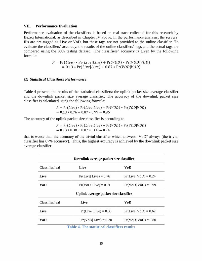
(1) Statistical Classifiers Performance

Table 4 presents the results of the statistical classifiers: the uplink packet size average classifier

and the downlink packet size average classifier. The accuracy of the downlink packet size

classifier is calculated using the following formula:

𝑃 = Pr(𝐿𝑖𝑣𝑒) ∗ Pr(𝐿𝑖𝑣𝑒|𝐿𝑖𝑣𝑒) + Pr(𝑉𝑂𝐷) ∗ Pr(𝑉𝑂𝐷|𝑉𝑂𝐷)

= 0.13 ∗ 0.76 + 0.87 ∗ 0.99 = 0.96

The accuracy of the uplink packet size classifier is according to:

𝑃 = Pr(𝐿𝑖𝑣𝑒) ∗ Pr(𝐿𝑖𝑣𝑒|𝐿𝑖𝑣𝑒) + Pr(𝑉𝑂𝐷) ∗ Pr(𝑉𝑂𝐷|𝑉𝑂𝐷)

= 0.13 ∗ 0.38 + 0.87 ∗ 0.80 = 0.74

that is worse than the accuracy of the trivial classifier which answers “VoD” always (the trivial

classifier has 87% accuracy). Thus, the highest accuracy is achieved by the downlink packet size

average classifier.

Downlink average packet size classifier

Classifier/real Live VoD

Live Pr(Live| Live) = 0.76 Pr(Live| VoD) = 0.24

VoD Pr(VoD| Live) = 0.01 Pr(VoD| VoD) = 0.99

Uplink average packet size classifier

Classifier/real Live VoD

Live Pr(Live| Live) = 0.38 Pr(Live| VoD) = 0.62

VoD Pr(VoD| Live) = 0.20 Pr(VoD| VoD) = 0.80

Table 4. The statistical classifiers results

26

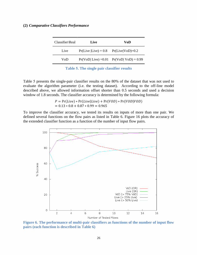
(2) Comparative Classifiers Performance

Classifier\Real Live VoD

Live Pr(Live |Live) = 0.8 Pr(Live|VoD)=0.2

VoD Pr(VoD| Live) =0.01 Pr(VoD| VoD) = 0.99

Table 5. The single pair classifier results

Table 5 presents the single-pair classifier results on the 80% of the dataset that was not used to

evaluate the algorithm parameter (i.e. the testing dataset). According to the off-line model

described above, we allowed information offset shorter than 0.5 seconds and used a decision

window of 1.8 seconds. The classifier accuracy is determined by the following formula:

𝑃 = Pr(𝐿𝑖𝑣𝑒) ∗ Pr(𝐿𝑖𝑣𝑒|𝐿𝑖𝑣𝑒) + Pr(𝑉𝑂𝐷) ∗ Pr(𝑉𝑂𝐷|𝑉𝑂𝐷)

= 0.13 ∗ 0.8 + 0.87 ∗ 0.99 = 0.965

To improve the classifier accuracy, we tested its results on inputs of more than one pair. We

defined several functions on the flow pairs as listed in Table 6. Figure 16 plots the accuracy of

the extended classifier function as a function of the number of input flow pairs.

Figure 6. The performance of multi-pair classifiers as functions of the number of input flow

pairs (each function is described in Table 6)

27

VoD (OR) Tag ‘VoD’ if all compares return ‘VoD’, otherwise ‘Live’

Live (OR) Tag ‘Live’ if at least 1 compare returns ‘Live’, otherwise ‘VoD’

VoD (> 75% VoD) Tag ‘VoD’ if at least 75% of compares return ‘VoD’, otherwise ‘Live’

Live (> 25% Live) Tag ‘Live’ if more than 25% of compares return ‘Live,’ otherwise ‘VoD’

Live (> 50% Live) Tag ‘Live’ if more than 50% of compares return ‘Live,’ otherwise ‘VoD’

Table 6. Description of multi-pair functions

Classifier\Real Live VoD

Live Pr(Live |Live) = 0.867 Pr(Live|VoD)=0.133

VoD Pr(VoD| Live) =0.00 Pr(VoD| VoD) = 1.0

Table 7. (> 25% Live) classifier results with 4 pairs

Table 7 presents the multi-pair classifier of 4 pairs compare with 'Live' if at list one pair tagged

'Live'. The test is on the 80% of the dataset that was not used to evaluate the algorithm

parameter. The classifier accuracy is determined by the following formula:

𝑃 = Pr(𝐿𝑖𝑣𝑒) ∗ Pr(𝐿𝑖𝑣𝑒|𝐿𝑖𝑣𝑒) + Pr(𝑉𝑂𝐷) ∗ Pr(𝑉𝑂𝐷|𝑉𝑂𝐷)

= 0.13 ∗ 0.86 + 0.87 ∗ 1.00 = 0.99

It can be seen that while adding more flow pairs to the classifier consideration, the accuracy

increases. However, adding more flow pairs decreases the classifier scalability due to the

additional matching operations that are required.

28

VIII. Conclusions

In this work, we emphasized the need for a classifier that distinguishes between the two video

streaming sub-classes: Live and VoD. Due to the massive use of video streaming in general and

Live video streaming in particular (as shown in [1]), Live streaming applications will require

special handling (e.g., by multicasting), which in turn will necessitate a reliable classifier.

We offered two such classifiers. We conducted a statistical analysis of our data collection and,

according to the results, we designed our statistical classifier. The performance evaluation of the

online statistical classifier showed that the highest accuracy achieved by such classifier is the

downlink packet size average classifier, with 96% accuracy. We also designed a comparative

classifier, which, while requiring at least one additional flow from the same source for

classification, yields superior results. The comparative classifier is based on the average time

difference between similar packets from two (or more) flows and shows accuracy between

96.5% and 97.53%, depending on the number of flows used for the comparison.

The comparative classifier presented a new approach which is different from the common

approach of DPI or any other statistical classification algorithms. While the perspective of other

classifiers was usually limited to a current packet or a single connection, our perspective in the

comparative classifier included multiple streams with common source. We examined several

options for multi-pair comparison which improved our results but decreased the solution

scalability.

The dataset collected for this research included Live and VoD streaming applications from one

streaming server each. To consolidate our solutions, there is room for testing them on more

traces from other streaming servers. These future traces should still be recorded in the ISP and

include many flows from each streaming server.

In Chapter VI, we showed that using multiple flows in our comparative classifier can enhance

the classifier results. However, this required many comparing operations and the solution became

cumbersome. Future work is needed in order to develop the multi-pair classifier to use many

flows at a decision window period without changing the solution scalability.

An additional option for enhancing the results is to combine the two classifiers (statistical and

comparative). As shown in Tables 4 and 5, the downlink statistical classifier achieved the best

results for Pr(Live |Live), while the comparative classifier achieved the best results for Pr(VoD| VoD).

As mentioned above, the statistical classifier required only a single flow while the comparative

classifier needed at least two flows for comparison. Therefore, a natural concept for future work

is to combine the two classifiers in a way that compares two flows and yet takes into account the

average packet size of each one.

29

IX. References

[1] Cisco Visual Networking Index (VNI): The Zettabyte Era, May 30, 2012, www.cisco.com

[2] F. Baker, B. Foster, and C. Sharp, “Cisco architecture for lawful intercept in IP networks,”

Internet Engineering Task Force, RFC 3924, 2004.

[3] S. Sen, O. Spatscheck, and D. Wang, “Accurate, scalable in network identification of P2P

traffic using application signatures,” in WWW2004, New York, NY, USA, May 2004.

[4] Bezeq International web site: http://www.bezeqint.net/

[5] V. Paxson. “Empirically derived analytic models of wide-area TCP connections”,

IEEE/ACM Transactions on Networking, August 1994.

[6] V. Paxson, and S. Floyd, “Wide area traffic: the failure of Poisson modeling”, IEEE/ACM

Transactions on Networking, June 1995.

[7] C. Dewes, A. Wichmann, A. Feldmann, An analysis of internet chat systems, in: IMC,

2003.

[8] M. Roughan, S. Sen, O. Spatscheck, N. Duffield, Class-of-service mapping for QoS: a

Statistical signature-based approach to IP traffic classification, in: IMC, 2004.

[9] D.M. Divakaran, H.A. Murthy, T.A. Gonsalves, Traffic modeling and classification using

packet train length and packet train size, in: IPOM , 2006.

[10] L. Bernaille, R. Teixeira, I. Akodjenou, A. Soule, K. Salamatian, Traffic classification on

the fly, in: ACM SIGCOMM Computer Communication Review, 2006.

[11] Ying-Dar Lin, Chun-Nan Lu, Yuan-Cheng Lai, Wei-Hao Peng, Po-Ching Lin, Application

classification using packet size distribution port association, Journal of Network and

Computer Applications (2009).

[12] Jayanthkumar Kannan, Jaeyeon Jung, Vern Paxson, Can Emre Koksal, Semi-automated

discovery of application session structure, in: IMC, 2006.

[13] T. Karagiannis, K. Papagiannaki, M. Faloutsos, BLINC: multilevel traffic classification in

the dark, in: Proceedings of the conference on applications, technologies, architectures, and

protocols for computer communications SIGCOMM, 2005.

[14] R. Nossenson, A. Lior and K. Brener, “On-Line Application Classification in Cellular

Backhaul Network”, In proceedings of the 17th IEEE International Conference on

Networks (ICON 2011), pp. 219-224, Singapore, Dec. 2011.

[15] H. Van Trees, Detection, estimation, and modulation theory. part 1, Wiley, New York,

1968.

30

תקציר

. הקובץ לטעינה מלאה שלללא צורך בהמתנה התחיל לצפות בסרט לט מאפשר לצופה נשידור וידאו באינטרניתן לחלק את השידורים . הקובץ ממשיך לרדת משרת המדיה, בזמן שהמשתמש צופה בקובץ המדיה

ובץ המדיה זמינים להורדה בכל שבו כל חלקי ק (VoD) דרישה יפל שידור ע: באינטרנט לשתי קטגוריותהוצעו מספר פתרונות לשיפור העברת . שמשודרים באותה העת זמינים להורדהושידור חי שבו רק החלקים ,עת

פתרונות אלו ממומשים אצל ספק האינטרנט ודורשים יכולת סיווג בין שידור חי . וידאו באינטרנט ברמת הרשתל ראשון מתבסס על מודהפתרון ה. זואנו מציגים שני פתרונות לבעיית סיווג עבודה זוב. לשידור לפי דרישה

הבדלי זמנים בין המסתמך עלשני מתבסס על מודל השוואתי הפתרון הגודל החבילות ו המסתמך עלסטטיסטי נאספו עבור בעזרת נתונים ש, וז עבודה המודלים המדוברים מוערכים ב. שונים לאותו שרת מדיה קישוריםשני

, הערכים הדרושים למסווגים לצורך למידתנעשה שימוש מהנתונים %02-ב. מחקר זה על ידי בזק בינלאומיהרצת המסווג הסטטיסטי על גבי הנתונים הראתה יכולת . הנותרים משמשים להערכת הביצועים %02-ש בעוד

בקשותמ %6.69 המדיה לעומת הרצת המסווג ההשוואתי שהראה יכולת זיהוי של בקשותמ %69 זיהוי שלשיפור . בקשותמספר רב יותר של ל התייחסותבנוסף הראינו דוגמאות לשיפור המודל ההשוואתי על ידי . המדיה

. אמנם המודל ההשוואתי נותן תוצאות מוצלחות יותר, הצלחה של סיווג אפליקציית המדיה %95.69 זה הראה כדי לסווג. נדרשת רק בקשה אחת בלבדמודל הסטטיסטי, בשונה מהמודל השוואתי, לאך

31

המרכז הבינתחומי הרצליה בית ספר אפי ארזי למדעי המחשב

( VoDוידאו על פי דרישה )בין סיווג מקוון שידור חילבין

המוגשת כמילוי חלק מהדרישות לקראת תואר תזה עבודת

מוסמך במסלול מחקרי במדעי המחשב

על ידי שובל פולצ'ק רונית נוסנסוןד"ר העבודה בוצעה בהנחיית

3102יוני