On viscous-inviscid interaction for boundary layer calculation using two-equation integral method

Ing. Vít Štorch

Supervisor: Prof. Ing. Jiří Nožička CSc.

Abstract A working viscous-inviscid interaction (VII) for boundary layer calculation does not only enhance the credibility and precision of results but also plays a crucial role in existence and calculation of solution of a two equation boundary layer model on geometry with transition and weak separation regions. The paper explains the importance of solving the boundary layer integral equations simultaneously or quasi-simultaneously with inviscid flow. A short overview of interaction methods is followed by some examples of the effects of VII on solutions. The overall goal of the presented work is to research possible ways of implementing the boundary layer model for different 2D and 3D panel methods being developed by the author. Key words Boundary layer, Viscous-inviscid interaction, integral method, transition, panel methods

1. Introduction In search of the most feasible approach to adding viscous effects to author’s expanding range of design tools based on panel methods and vortex lattice theory the integral two equation boundary layer model has been selected. The integral equation approach doesn’t require boundary layer discretization and seems to be a logical complement to panel methods that are BEM (boundary element methods) by nature. One of the well-established panel codes XFOIL by M. Drela [1] uses integral two-equation method. After thorough research of literature and implementation of the calculations it becomes clear that the viscous-inviscid interaction plays a key role in the integral two-equation model of boundary layer especially in cases with transition and weak separation regions. The simultaneous solution of boundary layer equations together with potential flow equations employed in the XFOIL code is a very complex and robust method with the disadvantage of placing severe constraints on panel code solver structure. Since the goal of the current study was to develop a „plug-in“ boundary layer calculation usable in several different applications including 2D airfoil analysis and cascade analysis, alternative approaches to treating viscous-inviscid interaction had to be explored.

2. Boundary layer formulation

2.1 Boundary layer integral equation parameters For solving integral equations, only the wall surface (boundary) needs to be discretized by i = 1÷N stations with coordinates ��. At each station, several boundary layer parameters together with chosen velocity profile family are required to describe the boundary layer. Among the parameters are: displacement thickness �∗, momentum thickness �, momentum thickness Reynolds number ���, kinetic energy thickness �∗, shape parameters H and H* , skin friction

coefficient Cf, dissipation coefficient CD and shear stress coefficient Cτ. The definition of these parameters is below. All integrals are across the boundary layer in η-direction perpendicular to surface. �∗ = �1 − ������ � �� (1.)

� = ������ �1 − ������ � �� (2.)

��� = ����� (3.)

�∗ = ������ �1 − �������� � �� (4.)

� = �∗� ; �∗ = �∗� (5.)

�� = 2������ (6.)

�� = 1��� � !�!� �� (7.)

�" = �#$%���� (8.)

2.2 Boundary equations The differential boundary layer equations are derived from full Navier-Stokes equations by using several simplifications and assumptions, such as constant pressure across the viscous layer and steady flow [2]: �% !�%!� + �' !�%!� = − 1� �(�� + ) !��%!�� (9.)

!�%!� + !�'!� = 0 (10.)

Among the first to derive and use integral equations were Kármán and Pohlhausen. Some methods use only the integral momentum equation, where the shape parameter is tied to the local pressure gradient. A representative example of such one-equation method is that of Thwaites[8]. As described in a paper by Drela and Giles [3] for separated flows a two-equation model is needed, so a modified two equation Green’s entrainment method was used for turbulent region in their ISES code. For laminar region a similar two-equation model only with different closure relation has been proposed for ISES.

This paper will be using the boundary layer formulation described in [3] only with some minor modifications, such as leaving out compressibility related terms. First equation is the integral momentum equation, the second equation is the kinetic energy shape parameter equation: ���� + �2 + �� ���

����� = ��2 (11.)

� ��∗�� + �∗�1 − �� ���

����� = 2�� − �∗ ��2 (12.)

The primary unknowns are H and θ. The edge velocity ue generally depends on the actual surface geometry and displacement thickness over the entire surface. It will be further investigated, but for current notation ue is assumed to be a function of local H and θ: �� = ����, �, ��,-� (13.)

The remaining parameters are tied by a series of closure relations that differ for laminar and turbulent boundary layer. �∗ = �∗��, ��, �� = ����, ��, �/ = �/��, �� (14.)

2.3 Laminar closure The following closure relations based on the Falkner-Skan profile family are valid in the laminar region: �∗ = 1.515 + 0.076 �4 − ���� , � ≤ 4

�∗ = 1.515 + 0.040 �� − 4��� , � > 4

(15.)

��� ��2 = −0.067 + 0.01977 �7.4 − ���� − 1 , � ≤ 7.4

��� ��2 = −0.067 + 0.022 81 − 1.4� − 69� , � > 7.4 (16.)

��� 2�/�∗ = 0.207 + 0.00205�4 − ��:.:, � ≤ 4

��� 2�/�∗ = 0.207 − 0.003 �� − 4��1 + 0.02�� − 4�� , � > 4 (17.)

For transition prediction the e^9 method first described by Smith and Gaberoni and also used in the ISES code [3] is employed. The transition theory is based on observing the spatial-amplification of small velocity perturbation at different frequencies. The key relation is the Orr-Sommerfeld equation describing the eigen modes and eigen frequencies of velocity oscillation in a viscous parallel stream [2]. The e^9 method assumes that the transition occurs when the most unstable wave has grown by a factor of e9=8103. The exponent 9 is valid for relatively turbulent flow usually found in wind tunnels [1]. Higher exponents should be used in strongly laminar incoming flows, for smooth surfaces and low vibrations – scenarios that delay

transition. In case of incoming flow with higher turbulence intensities and when vibrations or rough surface is a factor, lower exponents should be experimented with. An auxiliary transition equation for amplification ratio ñ is solved at each laminar station:

�ñ�� = �ñ����= + 12 ℓ 1� (18.)

Where: �ñ���� = 0.01?@2.4� − 3.7 + 2.5ABCh�1.5� − 4.65�E� + 0.25 (19.)

ℓ = 6.54� − 14.07�� (20.)

= = �0.058 �� − 4��� − 1 − 0.068� 1ℓ (21.)

When the amplification ratio at some point i reaches a critical value (ñi ≥ 9) the calculation continues with turbulent closure equations and point i is assumed the transition point.

2.4 Turbulent closure The following equations are used for the turbulent closure [3]: �∗ = 1.505 + 4��� + �0.165 − 1.6?���� ��G − ��� , � < �G

�∗ = 1.505 + 4��� + �� − �G�� I0.04� + 0.007JKL�����M� − �G + 4/JKL�����O�P , � > �G

�G = Q 4 (RK ��� < 400 3 + 400��� (RK ��� > 400

(22.)

�� = 0.3�ST. U@JKLTG�����EST.VWSG. TU + 0.00011 XABCℎ 84 − �0.8759 − 1Z (23.)

�� = ��2 [\ + �"�1 − [\� (24.)

[\ = �∗2 81 − 43 � − 1� 9 (25.)

The system of equations must be closed by one more relation for �". Green et. al. [5] proposed a method where the actual shear stress coefficient is calculated from its equilibrium value �" ]^ and its spatial rate of change: � _3.15 + � + 1.72� − 1`�"

��"�� = 4.2M�" ]^T/� − �" T/�O (26.)

Where: �" ]^ = �∗ 0.0151 − [\

�� − 1� � (27.)

3. Boundary layer solution method In laminar region, only two equations (11,12) are solved as a system of PDEs using Newton-Raphson iteration scheme. The amplification ratio is calculated after each iteration. In turbulent region, the additional equation for calculating shear stress must be calculated together with the integral equations. The equations (11,12,26) can be rewritten for Newton iteration method using central differencing (i-1/2): aT = �� − ��ST�� − ��ST + M2 + ��ST/�O ��ST/��� �ST/�

�� � − �� �ST�� − ��ST − �� �ST/�2 = 0 (28.)

a� = ��ST/� 8��∗�� 9�ST/�

�� − ��ST�� − ��ST + ��ST/�∗ M1 − ��ST/�O ��ST/��� �ST/��� � − �� �ST�� − ��ST− 2�� �ST/� + ��ST�∗ �� �ST/�2 = 0

(29.)

a = 2��ST/� 83.15 + ��ST/� + 1.72��ST/� − 19

�" �ST/�T/� �" �T/� − �" �STT/��� − ��ST− 4.2 _�" ]^ �ST/�T/� − �" �ST/�T/� ` = 0

(30.)

The calculation is marching downstream and the solution at each station is obtained in several iteration steps:

bccccd

!aT!��!aT!��

!aT!�" �T/�!a�!��!a�!��

!a�!�" �T/�!a !��!a !��

!a !�" �T/�effffg h ∆��∆��∆�" �T/�j = h−aT−a�−a j

(31.)

�� k]l = ∆�� + �� mn�; �� k]l = ∆�� + �� mn�; �" � k]lT/� = ∆�" �T/� + �" � mn�T/� (32.) The partial derivatives ∂f1, ∂f2 and (in turbulent region) ∂f3 are rather complex and will not be presented here.

4. Viscous – inviscid interaction methods

4.1 Selected 2D panel method for boundary layer implementation The boundary layer will be implemented into a simple 2D panel code for single airfoil analysis. It is expected that the findings and conclusions made using this setup are valid for other panel codes, such as 2D cascade panel method.

As a first step, inviscid solution must be obtained using the airfoil geometry and 2D panel method. The selected panel method uses a stream function formulation and linear vortex strength distribution. The surface is discretized by N points from the upper trailing edge across the leading edge to the lower trailing edge. The boundary condition is in form of a constant stream function on the surface. In practice the boundary condition is evaluated in nodal points, which form the panel edges. Unknowns are the vortex strengths pq in each nodal point and the surface value of stream function ΨG. For each nodal point, a linear equation can be formulated from the boundary condition [1]:

st�qpq

k

quT& �%vw� �'vx� ΨG 0,1 5 y 5 z (33.)

To complete the system of N+1 equations, Kutta condition is imposed on the trailing edge: pT & pk 0 (34.)

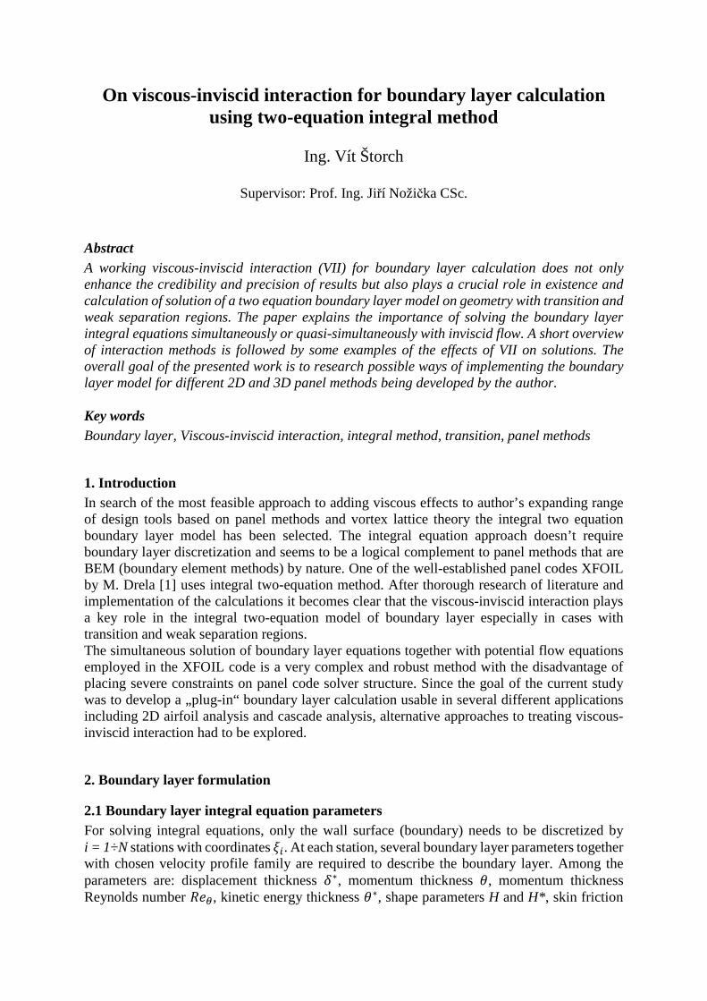
One of the benefits of the above formulation is the fact that surface velocity at each nodal point is equal to the vortex strength (�� {pq). The boundary model described earlier is in fact a 1D model not taking into account the surface curvature. Its application to the airfoil surface is shown in figure 1.

Fig. 1. Transformation from 2D boundary layer into 1D flat plate boundary layer problem

4.2 Viscous-inviscid interaction The main idea behind using potential flow solver for viscous flow is in dividing the flow field into inviscid region and viscous boundary layer (see fig. 2, top). Since the flow in the boundary layer is slower due to shear stress, this must be somehow taken into account by the potential solver. Shifting the solid wall outward in the normal direction to the wall using the displacement thickness value is one generally accepted method (see fig. 2, bottom). Other methods use wall transpiration techniques, where the boundary layer thickness is simulated by source singularities placed along the walls with a prescribed source strengths based on boundary layer thickness. The disadvantage of the second option is the fact that severe modifications must be

made to the flow solver if it does not use source panels, so the choice of the described method is the wall displacement technique.

Fig. 2. Solution of the boundary layer problem using displacement of the solid surface by the

displacement thickness value δ*. The boundary layer edge velocity ue at the border between viscous and inviscid region is taken to be identical to the surface velocity of inviscid solution using the modified geometry. The relatively complex calculation of boundary layer equations in our case using downstream marching must therefore share δ* and ue with the potential flow solver, which is solved at once using linear system of equations. The sharing of displacement thickness δ* and edge velocity ue values is called viscous-inviscid interaction or also boundary layer coupling.

4.3 Methods of viscous-inviscid interaction The simplest method of boundary layer coupling is no interaction at all. First the edge velocity is calculated using panel method and then the boundary layer is solved with the prescribed edge velocity as a constant. If the thickness and its variations are very small, this method was expected to give reasonable results. For true viscous-inviscid interaction methods Veldman [6] suggests the following types arranged by complexity:

• Direct method: Intuitive technique where the potential flow solver calculates edge velocity, the boundary layer solver calculates the displacement thickness, the geometry is changed to account for the BL thickness and the whole process is repeated in several iteration steps.

• Inverse method: The same procedure as with direct method is followed with the only difference that the potential solver is modified to inverse mode where it calculates geometry (displacement thickness), whereas the boundary layer solves for edge velocity, based on given δ* distribution.

• Quasi-simultaneous method: A simplified relation between δ* and ue is used together with the boundary equations. Several iteration loops with subsequent BL and potential flow calculations are still needed, the main difference with respect to the direct method

is the fact that both δ* and ue are variables, which brings some important benefits as will be described in section 4.4.

• Full simultaneous method: The boundary layer equations are solved together with potential flow in one system of equations. The wall transpiration technique is beneficial in this case. XFOIL [1] uses such layout.

4.4 Strong interaction, separation and Goldstein singularity In case of an attached laminar flow, the boundary layer grows gradually in thickness which presents a weak interaction problem. When the flow approaches separation, traditional integral methods face difficulties in producing valid solution as was first described by Goldstein in 1948 [7]. The Goldstein singularity refers to the singularity of solution near separation point at the trailing edge of the airfoil using traditional one-equation downstream marching boundary layer algorithms. The issues with singularity are faced generally whenever there is strong interaction between the boundary layer and potential flow. This includes laminar boundary layer separation (usually followed by transition and reattachment - laminar bubbles), transition and trailing edge separation. Full laminar or turbulent separation without reattachment can be classified also as a strong interaction, but cannot be handled by the presented boundary layer theory. In region of strong interaction only a certain range of edge velocities will result in a valid solution whilst for a fixed ue distribution no solution may exist. Some attempts to circumvent this problem include inverse formulation with prescribed thickness and variable ue or even prescribed Cf and variable δ* and ue [4]. A robust remedy to the singularity problem is to use two-equation model valid near separation point (such as the one used in this paper) and to adopt either quasi-simultaneous or simultaneous approach for solving the boundary layer equations. The quasi-simultaneous method is further explored since it promises a ‘portable solution’ for the boundary layer that can be used in several different cases without altering the flow solver.

5 Quasi-simultaneous methods

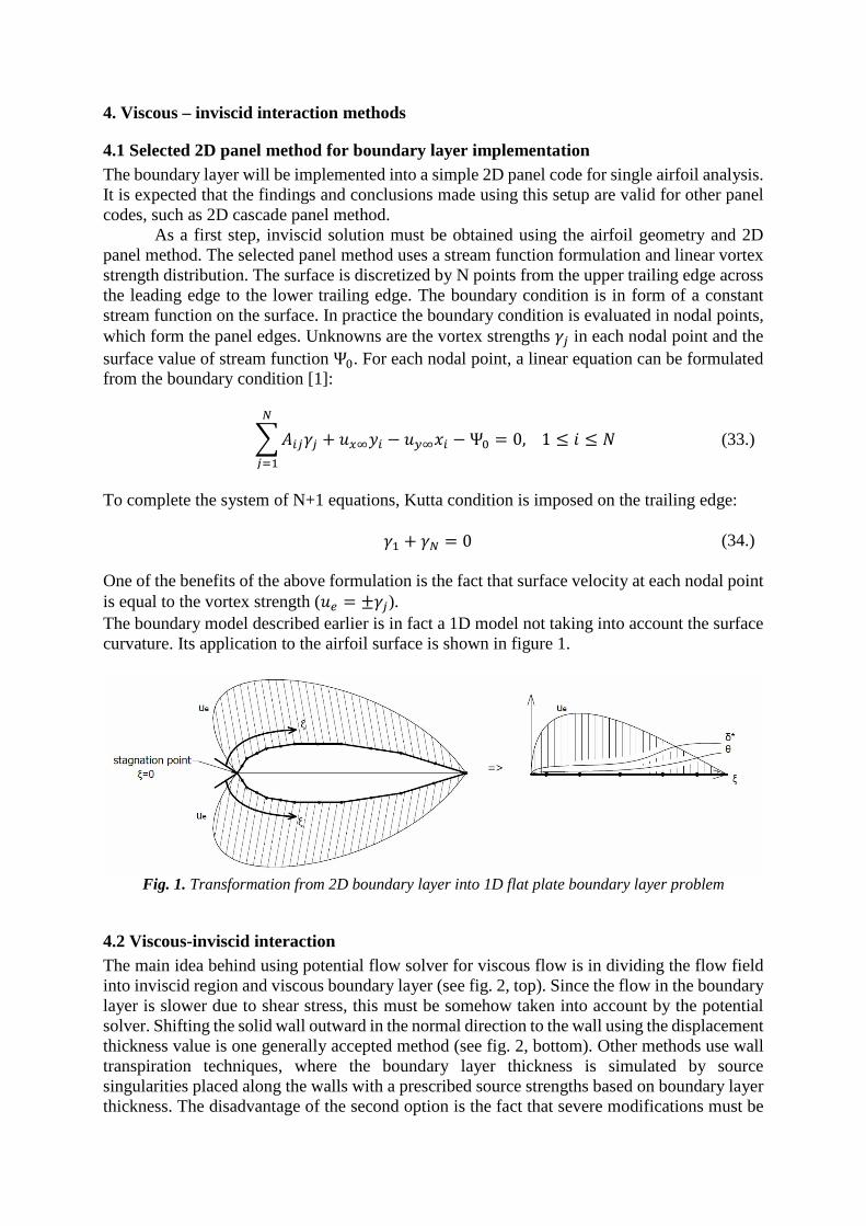
The goal of quasi-simultaneous methods is to present a simplified δ* - ue relation. In the potential solver based on panel method the slightest change of δi* leads to i-th panel node being displaced in the geometry, which results in changes in the influence coefficient matrix t�q throughout i-th row and i-th column. Solving the modified system of equations results in a new velocity distribution that differs from the old one at every node. It follows that a local geometry modification realised by change of δi* influences the entire solution (fig. 3). Based on this observation, one common and several alternative interaction methods are tested.

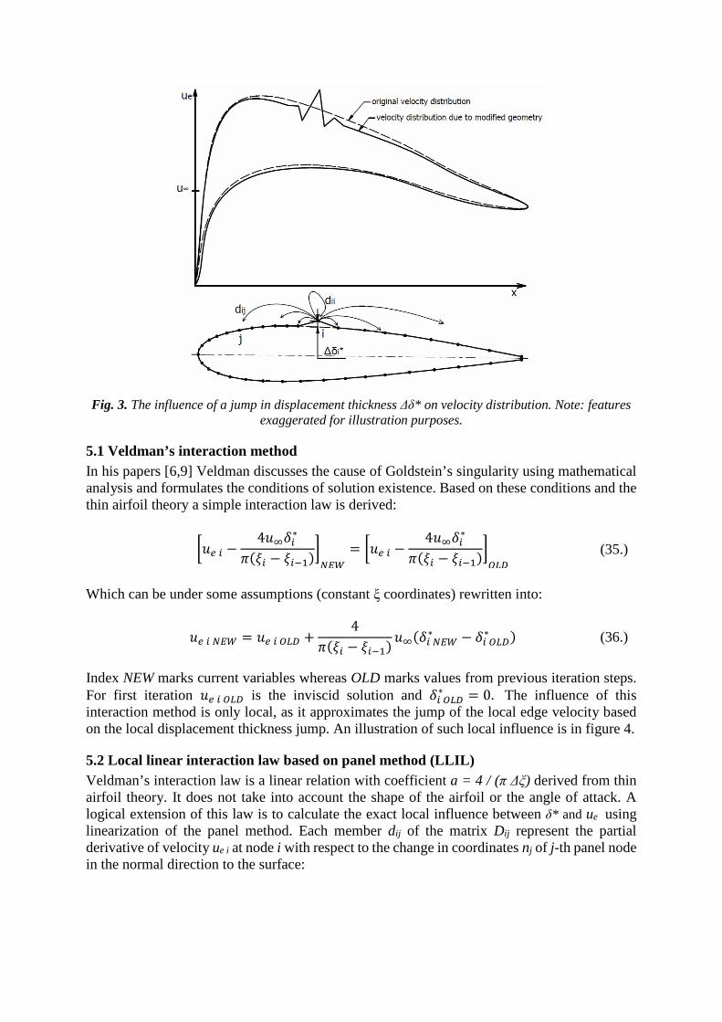
Fig. 3. The influence of a jump in displacement thickness Δδ* on velocity distribution. Note: features

exaggerated for illustration purposes.

5.1 Veldman’s interaction method In his papers [6,9] Veldman discusses the cause of Goldstein’s singularity using mathematical analysis and formulates the conditions of solution existence. Based on these conditions and the thin airfoil theory a simple interaction law is derived: X��� 4�v��∗|��� ��ST�Zk]l X��� 4�v��∗|��� ��ST�Zmn� (35.)

Which can be under some assumptions (constant ξ coordinates) rewritten into: ���k]l ���mn� & 4|��� ��ST� �v���k]l∗ ��mn�∗ � (36.)

Index NEW marks current variables whereas OLD marks values from previous iteration steps. For first iteration ���mn� is the inviscid solution and ��mn�∗ 0. The influence of this interaction method is only local, as it approximates the jump of the local edge velocity based on the local displacement thickness jump. An illustration of such local influence is in figure 4.

5.2 Local linear interaction law based on panel method (LLIL) Veldman’s interaction law is a linear relation with coefficient a = 4 / (π Δξ) derived from thin airfoil theory. It does not take into account the shape of the airfoil or the angle of attack. A logical extension of this law is to calculate the exact local influence between δ* and ue using linearization of the panel method. Each member dij of the matrix Dij represent the partial derivative of velocity ue i at node i with respect to the change in coordinates nj of j-th panel node in the normal direction to the surface:

}�q 1�vbcccd!�T!CT … !�T!Ck⋮ !��!Cq!�k!CT

!�k!Ckefffg (37.)

For local linear interaction method, only the influence of the panel node displacement on its local edge velocity is needed, so only the diagonal members dii will be used in this method. The resulting relation is similar to Veldman interaction law, only more accurate and also more computationally expensive due to Dij matrix calculation: ���k]l ���mn� & ��� �v���k]l∗ ��mn�∗ � (38.)

Fig. 4. The simplified influence of a jump in displacement thickness Δδ* on velocity distribution using

Veldman’s interaction law.

5.3 Global downstream linear interaction law based on potential flow solver (GDLIL) Since the whole δ* - ue influence matrix Dij is available, the following update of all downstream ��mn� values is possible after the solution converges at node i:

aKR� ∈ ��y & 1�, . . . , z���qmn� ��qmn� & ��q�v���k]l∗ ��mn�∗ � (39.) During Newton iteration procedure at each node the same LLIL interaction law as described previously (section 5.2) is used. The update of ��mn�values only affects the downstream nodes. It follows that ��qmn� value at j-th node will be updated (j-2) times, since the calculation

marches from node 2 to node j-1 before reching the j-th node. Upstream node ��mn�values are left unchanged, since the calculation runs only in the downstream direction.

6. Results

6.1 Flat plate, no interaction Experiments with the two-equation boundary layer calculation confirmed that only small number of cases with no interaction law converged, all of which were variations of flat plate with constant edge velocity, or very subtle velocity gradients. This also means that the described BL model is not suitable for direct or inverse coupling, since the calculation breaks up during first pass through the boundary layer. The results for flat plate with no interaction are below:

Fig. 5. Calculation results for flat plate with no interaction law

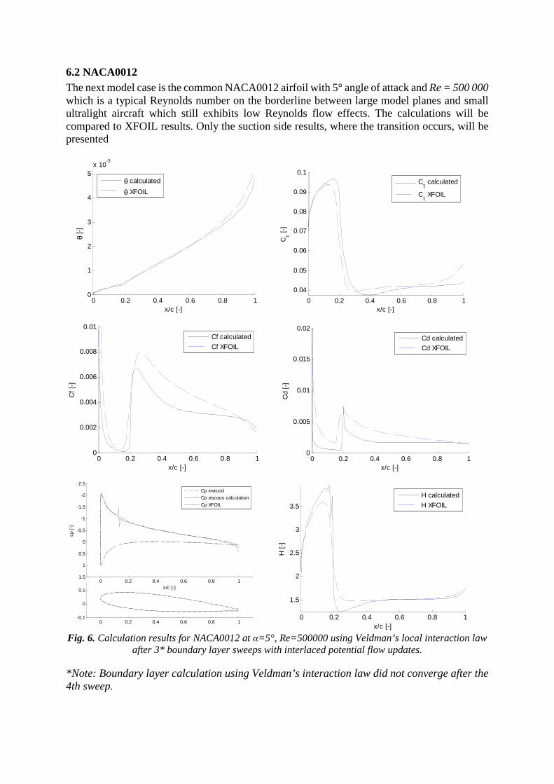
6.2 NACA0012 The next model case is the common NACA0012 airfoil with 5° angle of attack and Re = 500 000 which is a typical Reynolds number on the borderline between large model planes and small ultralight aircraft which still exhibits low Reynolds flow effects. The calculations will be compared to XFOIL results. Only the suction side results, where the transition occurs, will be presented

Fig. 6. Calculation results for NACA0012 at α=5°, Re=500000 using Veldman’s local interaction law

after 3* boundary layer sweeps with interlaced potential flow updates.

*Note: Boundary layer calculation using Veldman’s interaction law did not converge after the 4th sweep.

0 0.2 0.4 0.6 0.8 10

1

2

3

4

5x 10

-3

x/c [-]

θ [-

]

θ calculated

θ XFOIL

0 0.2 0.4 0.6 0.8 1

0.04

0.05

0.06

0.07

0.08

0.09

0.1

x/c [-]

Cτ [

-]

Cτ calculated

Cτ XFOIL

0 0.2 0.4 0.6 0.8 10

0.002

0.004

0.006

0.008

0.01

x/c [-]

Cf

[-]

Cf calculated

Cf XFOIL

0 0.2 0.4 0.6 0.8 10

0.005

0.01

0.015

0.02

x/c [-]

Cd

[-]

Cd calculated

Cd XFOIL

0 0.2 0.4 0.6 0.8 1-0.1

0

0.1

0 0.2 0.4 0.6 0.8 1

-2.5

-2

-1.5

-1

-0.5

0

0.5

1

1.5

x/c [-]

cp [

-]

Cp inviscid

Cp viscous calculation

Cp XFOIL

0 0.2 0.4 0.6 0.8 1

1.5

2

2.5

3

3.5

x/c [-]

H [

-]

H calculated

H XFOIL

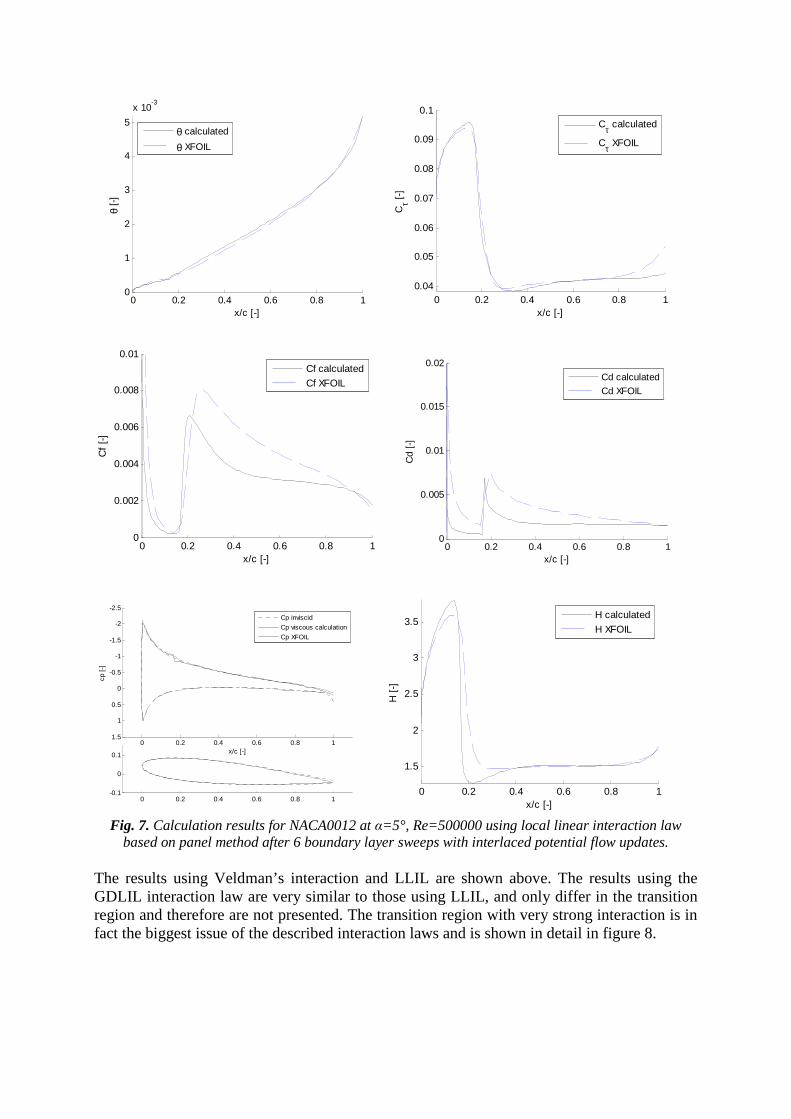
Fig. 7. Calculation results for NACA0012 at α=5°, Re=500000 using local linear interaction law

based on panel method after 6 boundary layer sweeps with interlaced potential flow updates. The results using Veldman’s interaction and LLIL are shown above. The results using the GDLIL interaction law are very similar to those using LLIL, and only differ in the transition region and therefore are not presented. The transition region with very strong interaction is in fact the biggest issue of the described interaction laws and is shown in detail in figure 8.

0 0.2 0.4 0.6 0.8 10

1

2

3

4

5

x 10-3

x/c [-]

θ [-

]

θ calculated

θ XFOIL

0 0.2 0.4 0.6 0.8 10.04

0.05

0.06

0.07

0.08

0.09

0.1

x/c [-]

Cτ [

-]

Cτ calculated

Cτ XFOIL

0 0.2 0.4 0.6 0.8 10

0.002

0.004

0.006

0.008

0.01

x/c [-]

Cf

[-]

Cf calculated

Cf XFOIL

0 0.2 0.4 0.6 0.8 10

0.005

0.01

0.015

0.02

x/c [-]

Cd

[-]

Cd calculated

Cd XFOIL

0 0.2 0.4 0.6 0.8 1-0.1

0

0.1

0 0.2 0.4 0.6 0.8 1

-2.5

-2

-1.5

-1

-0.5

0

0.5

1

1.5

x/c [-]

cp [

-]

Cp inviscid

Cp viscous calculation

Cp XFOIL

0 0.2 0.4 0.6 0.8 1

1.5

2

2.5

3

3.5

x/c [-]

H [

-]

H calculated

H XFOIL

Fig. 8. Details of transition region of cp diagram. Top left: Veldman’s interaction law, Top right:

LLIL, Bottom left: GLIL. Calculation results for NACA0012 at α=5°, Re=500000

7. Conclusion The relatively complex two equation integral method chosen for boundary layer calculation has some advantages in terms of behavior at and near separation. However, correct coupling to the flow solver is required for the solution to converge. After ruling out simultaneous interaction method for its complexity, several interaction laws for quasi-simultaneous calculations were tested. Veldman’s interaction law is based on calculating a simple local linear relation between displacement thickness and edge velocity. This relation is based solely on local panel size regardless of the panel position, orientation and airfoil shape and does not present any further computational effort. Calculation of the boundary layer successfully converges after using Veldman’s interaction law, however erratic velocity distribution exists in the transition region which only grows with subsequent BL sweeps until the solution diverges. The next logical step was to determine the precise local linear relation based on the actual airfoil geometry using the panel method (marked as LLIL interaction law). Using this law, unlimited sweeps of the boundary layer are possible, due to the interaction law working correctly even in the transition region. Higher number of iterations (sweeps) also result in the solution being closer to the reference XFOIL data. The transition region edge velocity distribution still lacks the smoothness of XFOIL solution so an attempt was made to correct this behavior by developing a global downstream linear interaction law (GDLIL), where the downstream edge velocities are updated as the calculation marches from the stagnation point towards trailing edge. The effect on transition smoothness was positive but almost negligible, the main improvement being faster convergence (fewer BL sweeps required) especially for the region closer to trailing edge. Since the region near leading edge must converge as well, the advantage of such behavior is questionable. Based on the above discussion the coupling method of choice for future implementation of BL model is the LLIL interaction law. Effective ways of calculating the velocity influence matrix Dij should be researched for speeding up the calculation process. A mix of Veldman’s interaction law across most of the airfoil and LLIL at the transition region could combine the best of both methods. Also the full Dij matrix could be potentially used for a fully simultaneous method. These are possible directions of the future research.

List of symbols Aij Influence coefficient matrix for stream function formulation (m) c Chord length (m) cp Coefficient of pressure (1) Cd Dissipation coefficient (1) Cf Friction coefficient (1) Cτ Shear stress coefficient (1) Dij Influence coefficient matrix for velocity formulation (m-1) H Shape parameter (1) H* Kinetic energy shape parameter (1) n Panel normal (m) N Number of panel nodes (1) Reθ Momentum thickness Reynolds number (1) u u∞, uinv, ue – velocity at infinity, inviscid and edge velocity (m·s-1) x Coordinate along the chord (m) α Angle of attack ( º ) ξ, η Airfoil surface coordinates (ξ – tangent, η - normal) (m) Ψ Stream function (m2·s-1) γ Specific vortex strength (m·s-1) δ* Displacement thickness (m) θ Momentum thickness (m) θ* Kinetic energy thickness (m) ρ Density (kg·m-3) ñ Amplification ratio (1) References [1] Drela M.: XFOIL: An Analysis and Design System for Low Reynolds Number Airfoils, Low Reynolds Number Aerodynamics, Springer-Verlag Lec. Notes, Eng. 54. 1989

[2] Schlichting H., Gersten K.: Boundary-layer theory. Berlin New York: Springer, 2000, ISBN 3-540-66270-7

[3] Drela M., Giles M.: Viscous-Inviscid Analysis of Transonic and Low Reynolds Number Airfoils, AIAA Journal, Vol. 25, No. 10. 1987

[4] Johansen J.: Prediction of Laminar/Turbulent Transition in Airfoil Flows, Risø-R-987(EN), 1997

[5] Green J., Weeks D. and Brooman J.: Prediction of Turbulent Boundary Layers and Wakes in Compressible Flow by a Lag-Entrainment Method. Report no. 3791, HMSO, London, 1977

[6] Bijleveld H.,Veldman A.: Prediction of unsteady flow over airfoils using a quasi-simultaneous interaction method, Wind Energy, 2013

[7] Veldman A.: Viscous-Inviscid Interaction: Prandtl’s Boundary Layer challenged by Goldstein’s Singularity, 2004, pdf available: http://www.math.rug.nl/~veldman/preprints/BAIL2004.pdf

[8] Thwaites B.: Incompressible Aerodynamics, Clarendon Press, Oxford, 1960

[9] Veldman A.: A simple interaction law for viscous-inviscid interaction. Journal of Engineering, Mathematics, 65:367–383, 2009.

Acknowledgements: The work was supported by the Grant Agency of the Czech Technical University in Prague, grant No. SGS 15/065/OHK2/1T/12.