on the use of euler and crank-nicolson time-stepping

On the use of Euler and Crank-Nicolson time-stepping schemes for seakeeping simulations in OpenFOAM

VII International Conference on Computational Methods in Marine EngineeringMARINE 2017

M. Visonneau, P. Queutey and D. Le Touze (Eds)

ON THE USE OF EULER AND CRANK-NICOLSONTIME-STEPPING SCHEMES FOR SEAKEEPING

SIMULATIONS IN OPENFOAM R©

Sopheak Seng∗, Charles Monroy, Sime Malenica

Bureau Veritas, Marine & Offshore DivisionResearch Department, 92571 Neuilly-sur-Seine, France

∗e-mail: [email protected]

Key words: Seakeeping, OpenFOAM, VOF, Crank-Nicolson, Euler

Abstract. The open-source CFD software package OpenFOAM has reached a maturity levelsuch that it is possible to perform seakeeping simulations using the included VOF-based free-surface URANS (Unsteady-Reynolds-Averaged Navier-Stokes) solver (a.k.a interDyMFoam).This paper describes results of seakeeping tests and the experiences obtained while selectingan appropriate combination of spatial and temporal schemes for wave and seakeeping simula-tions in a regular head sea condition. Particular attention has been paid to the accuracy leveland the convergence rate of temporal schemes Euler and CrankNicolson since an accurate tem-poral discretization is known to be very important for wave propagations. Here the numericalresults confirm the need for at least a 2nd-order temporal scheme. To improve the stability andthe robustness of the existing CrankNicolson scheme we customized the code and performed anumerical experiment on the modified CrankNicolson scheme where the off-centering parameterco is non-uniformly distributed in the domain. The results show that when using a simple distri-bution of the co parameter the stability of the CrankNicolson scheme can be restored withouthaving to degrade significantly the numerical order of the scheme. This new approach allowsstable simulations to be performed where the incident wave field is propagated more acceptablywith a very small decay and, at the same time, keeps the time step large enough to allow thesimulations to finish at a reasonable CPU time.

1 INTRODUCTION

The study of ship motion in waves is commonly performed using tools based on potentialflow theory which are very efficient in linear waves but cannot account sufficiently for highlynonlinear waves, strong body nonlinearity, high Froude-number and the viscous effects. Inthe hope of overcoming these issues simulations based on a free-surface URANS (UnsteadyReynolds-Averaged Navier-Stokes) solver is becoming increasingly more popular since the solverand the necessary seakeeping capabilities are available in commercial codes as well as in open-source codes. One of the critical components for seakeeping simulations is the capability togenerate waves and propagate them accurately toward the ship. Hence, one of the preliminary

1

905

Sopheak Seng, Charles Monroy and Sime Malenica

steps to evaluate a free surface URANS code for its seakeeping capability is to establish practicalexperiences on how wave systems and perhaps more fundamentally the dynamics and kinematicsof the free surface can be simulated efficiently and accurately. Physically, besides the incidentwave field there are several important wave systems generated by the presence of the ship and itsmotion. For example, at a certain combination of low Froude numbers and wave frequencies theradiated and diffracted waves are propagating upstream ahead of the ship creating a complicatedinterfering pattern with the incident wave field. These wave systems travel very far from theship. Since most of the free surface URANS codes need a finite computational domain the wavesystems may cause stability problems, numerical artifacts at wave generation boundaries and acertain level of artificial wave reflection from the truncated boundaries.

The work done in this paper uses the open-source software package OpenFOAM [1, 2] witha necessary customized third-party wave library based on [3] to introduce waves into the com-putational domain. The objective of the work is to evaluate from a practical point of view therobustness, the efficiency and the accuracy of the public domain OpenFOAM code for seakeep-ing simulations. A seakeeping case in a head sea condition in a long crested regular wave isselected for the purpose. The configuration of the seakeeping mesh is selected appropriatelyto include sufficient refinements within the free surface zone, the wave propagation zone, thewave damping zone and the near-hull local regions. The errors related to the propagation ofthe regular incident wave field on this selected mesh configuration are first evaluated before per-forming the full seakeeping simulation. The flow solver uses the FVM (Finite Volume Method)discretization for solving URANS equations and the free surface is captured by a VOF (Volumeof Fluid) method. The capability to generate and absorb waves is added according to [3]. Themathematical formulation and the important aspects of this solver are presented in Sec. 2 be-low. Two test conditions are presented. The first test condition is for the propagations of theincident wave field on a 2D mesh with a similar configuration as for the 3D seakeeping mesh.This test condition shall provide a good insight on how well the simulated incident wave fieldcan be propagated from the wave inlet boundary toward the ship. The second test conditionis the 3D seakeeping test performed with similar numerical schemes and configuration takenfrom the best known 2D wave tests. The general numerical setup is described in Sec. 3 and theresults of the simulations are discussed in Sec. 4.

2 NUMERICAL MODEL

The OpenFOAM software package is a collection of C++ libraries which provide core func-tionalities for solving partial differential equations. One of its most developed functionalities isthe FVM discretization using unstructured polyhedral meshes. Several basic solvers are includedin the package. The flow solver used in this work is a VOF based incompressible two-phase solver.It solves the URANS equations and a modified transport equation of the phase fraction field.Details related to the basic principle of VOF can be found in [6]. Air and water are consideredimmiscible and treated as viscous and incompressible. While the computational domain includesboth air and water with a density ratio up to approximately 1000, the mass and momentumconservation are formulated under the assumption that the density ρ and viscosity µ of theeffective fluid can be computed using the volume phase fraction field as weighting factor as in

2

906


Eq. (1) below:

ρ = αρw + (1− α)ρa (1)

µ = αµw + (1− α)µa

where the subindices ”a, w” indicate air and water, respectively. The volume phase fractionfield α must be bounded between 0 and 1 since it describes the volume fraction of water in thecontrol volume. Here the surface tension is considered negligible. The governing equations forthe laminar model (the turbulence model is runtime selectable) including the modified transportequation read

∇ · u = 0 (2)

∂α

∂t+∇ · αu+∇ · [α(1− α)ur] = 0 (3)

∂ρu

∂t+∇ · ρuuT −∇ ·

[µ(∇u+∇uT )

]= −∇prgh − (g · x)∇ρ (4)

The pressure field prgh is defined in relation to the static pressure p as prgh ≡ p− ρg · x, whereg is the vector representing the gravitational acceleration and x is the position vector. Thevelocity/pressure coupling is resolved in time using a modified PISO algorithm known to theOpenFOAM community as the PIMPLE algorithm which is a unified implementation of the PISOalgorithm (pressure-implicit with split-operator [7]) and the SIMPLE algorithm (Semi-ImplicitMethod for Pressure Linked Equations). Through user-selected run-time controlling parametersthe PIMPLE algorithm can be configured to operate in pure PISO or SIMPLE mode. Moreimportantly it enables a combined use of SIMPLE/PISO mode (a.k.a PIMPLE mode) to achievea more efficient time stepping since in this mode the time step size shall be less constrained thanin the PISO mode. The PIMPLE mode has been used in all simulations performed this work.

To keep the α-field bounded between 0 and 1, Eq. (3) is solved using the semi-implicitMULES solver (Multidimensional Universal Limiter with Explicit Solution). Although MULEShas been introduced into the OpenFOAM library almost a decade ago the literature on thissolver is sparse. The work done in [8, 9] are examples of recent efforts to describe the MULESsolver. The ability of MULES in keeping the α-field bounded is documented in [9]. The artificialterm in Eq. (3) (the third time on the left-hand-side) is added in an attempt to prevent smearingof the interface due to numerical diffusion in the α-field. This term is designed to compress theinterface by adding artificial flux to the equation and requires an empirical model for ur (seealso [10]), the relative velocity between the air and water, which in theory should be zero but inpractice is different from zero due to the numerical smearing and the difficulty of representingthe interface exactly in the VOF formulation. The treatment of the transport equation for theα-field using this artificial term in a combination with the MULES solver can be classified asan algebraic VOF algorithm. While it is possible to obtain good results with this algorithm theconclusion put forward by [9] is that MULES is inferior to geometric VOF algorithms. Since theOpenFOAM software package does not provide other options, the current work uses exclusivelythe semi-implicit MULES in all simulations.

The FVM discretization of the governing equations is managed by the OpenFOAM corelibrary which follows the standard FVM practice of converting volume integrals to surface in-tegrals using Gauss’s theorem. The integration and interpolation scheme for each term in the

3

907


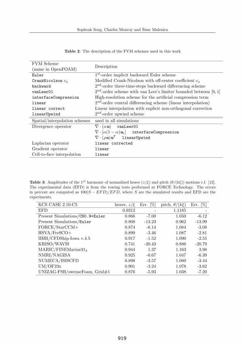
equations are made runtime selectable. These include the time derivative term for the mo-mentum equation and the transport equation, the divergence and the gradient operators. The2nd-order upwind scheme has been selected for the convective term in the momentum equationsand the 2nd-order central differencing scheme for the diffusive term. The α-field always hasa steep gradient near the free surface. Hence, the 2nd-order high-resolution shock capturingscheme van Leer is selected for the convective term in the transport equation for the α-field.For the time derivative terms OpenFOAM core library provides three different schemes named:Euler, backward, and CrankNicolson. The Euler scheme in OpenFOAM is an implementationof the backward Euler integration algorithm which is implicit and known to be very stable butonly 1st-order accurate. The numerical results of wave propagations which are presented anddiscussed in Sec. 4.1 show that the Euler scheme, although very stable, is 1st-order accurate andis not sufficient for propagating waves from the wave generation boundaries toward the ship. Tomaintain an acceptable wave condition within the vicinity of the ship the order of the temporalscheme needs to be at least 2nd-order accurate which can be achieved using either backward orCrankNicolson. In OpenFOAM backward is the 2nd-order three-time-steps backward differen-tiation formula and CrankNicolson is a modified Crank-Nicolson scheme where an off-centerparameter with a value between 0 and 1 has been introduced to control the weight toward eitherstandard Crank-Nicolson scheme or the implicit Euler scheme. It appears that the backward orthe CrankNicolson schemes can be readily applied to obtain a 2nd-order integration in time.However, the backward scheme is known to be unbounded. Hence it cannot be applied to thetransport equation for the α-field since it will cause extreme difficulty to control a boundedsolution of the α-field to within 0 and 1. The option to use the backward scheme in MULESis simply disabled. The CrankNicolson scheme, on the other hand, can be made boundedand is supported by MULES to obtain a consistent 2nd-order temporal accuracy not only forthe momentum equations but also for the transport equation of the α-field. The simulationperformed in this work, however, quickly reveals that the CrankNicolson scheme may causethe numerical solution to have an oscillatory convergence. When the scheme is used directlyin FSI (fluid structure interaction) simulations where the body motion is resolved through apartitioning scheme where the flow solver and the body-motion solver are executed alternately(with fixed under-relaxation of the body acceleration) the oscillatory flow solutions are havinga strong negative influence on the convergence behavior of the FSI iterations. When the FSIconverges, the number of FSI iterations increases significantly. Under certain circumstances theFSI iterations diverges. The oscillatory convergence behavior of the CrankNicolson scheme iswell known and the oscillatory behavior is associated with a too large Courant number (C � 1).Under normal circumstances the Courant number is computed as the global maximum whichis conservative since the Courant number is critically high at a few local cells only. Thesecells are typically inside local refinement regions where the cells are very small due to eitherphysical constraints such as boundary layer flow and the selected turbulence model or technicalissues related to automatic mesh generations. The latter seems evident when using automaticmesh generation tools which are based on unstructured split-hexahedra. These are e.g. the freelyavailable snappyHexMesh1 or similar commercial alternatives such as HEXPRESSTM or STAR-CCM+.

1A utility provided by the OpenFOAM software package to generate unstructured 3-dimensional meshes con-taining mostly hexahedra and spitted hexahedra

4

908


Assuming that these critical small cells region are an unavoidable product of the automatic meshgeneration tools and the physics of the flow within these regions do not require the cells to be sosmall it is natural to think of a solution to trade on the unnecessarily high spatial resolution foran increasing numerical stability. One of the easiest solution which is put under a numerical ex-periment in this paper is to adjust locally the off-center parameter found in the CrankNicolsonscheme. In OpenFOAM the implementation of this solution is straightforward costing no morethan a few lines of codes added to the source code of the flow solver. Here this solution shall bedescribed in detail.

Recall that the standard Crank-Nicolson scheme can be viewed as a half-and-half weightingbetween the forward and backward Euler-schemes, the weight coefficient can be considered as anadjustable parameter which controls the numerical behavior of the scheme. In OpenFOAM thisweighting coefficient has been implemented as described below. Consider the following generic1st-order ODE (ordinary differential equation)

y = f(t, y) (5)

According to the forward Euler scheme the integration from time step n to n+1 is approximatedby yn+1−yn ≈ hfn where h = tn+1−tn is the time step size and fn = f(tn, yn). For the backwardEuler scheme the approximation is yn+1 − yn ≈ hfn+1. A weighting coefficient γ = [0, 1] hasbeen introduced as follows:

yn+1 − yn ≈ γhfn+1 + (1− γ)hfn (6)

For γ = 1/2 the scheme is equivalent to the standard Crank-Nicolson scheme. The scheme canbe made equivalent to the forward explicit Euler scheme by selecting γ = 0. For stability reason,however, it is advisable to keep γ between 1/2 and 1, where γ = 1 is equivalent to the fullyimplicit 1st-order backward Euler scheme. In OpenFOAM γ can be adjusted within the range ofγ = [1/2, 1]. The adjustment is made available during run-time through an off-center coefficientco which is related to γ as follows

co ≡1− γ

γfor γ = [0.5, 1] (7)

From this definition co will have a value between 0 and 1. The standard 2nd-order Crank-Nicolson scheme (γ = 0.5) is specified as co = 1, and the implicit 1st-order backward Euler(γ = 1) as co = 0. It is noted that a 2nd-order accuracy can be expected only by using co = 1(i.e. γ = 0.5). Clearly if the simulation runs stable at co = 1 it will not be wise to lower thiscoefficient. Changing the value of co slightly, says co = 0.9, will increase numerical dissipationand reduce the order toward the fully 1st-order backward Euler. The lost of accuracy shall bejudged against the benefit of having an additional numerical dissipation which means betternumerical stability. In cases the simulations cannot proceed at co = 1 due to stability reasonsthis additional dissipation may become very valuable if it restores fully the numerical stabilitywith a minimal and local impact on the flow features of interest. In seakeeping the flow featuresof interest, preliminarily, are the wave field at the position of the ship. From this point of viewit is justifiable to allow a non-constant spatial dependency of the co parameter if the benefit ofadded numerical stability outweighs the lost of accuracy. Obviously it is not trivial to determine

5

909


Ref. 1 Ref. 3cells are stretched vertically

in the free surface zonewave inlet BCOu

tlet B

CRef. 2 wave propagation zoneFPAP MS

wave damping zone ( ) slip BC on the bottom

Figure 1: A sketch of the mesh configuration and the boundary conditions (BC) defined in the 2D wavetests (without the ship). The longitudinal position of the ship is indicated by AP (aft perpendicular),MS (midship) and FP (forward perpendicular). The wave length is λ ≈ 11.84 m c.f. Table 1.

an optimum spatial dependency for co. The first aims, however, is not to have a fully optimaldistribution for co but to establish some evidences showing that the benefit of having a non-constant spatial distribution of co can be achieved in practice. The numerical experimentsconstructed in this paper shall provide more insight on this subject.

3 NUMERICAL SETUP

It is generally acknowledged that seakeeping simulations based on a FVM free-surface URANSsolver are computationally very expensive which provides a strong motivation for keeping thecell count low. The seakeeping mesh is generated using unstructured body-fitted split-hexahedramesh. Waves are introduced into the domain by imposing wave kinematics and free surface con-ditions at the wave generation boundaries. To prevent wave reflection from the outlet boundarywe use an explicit relaxation zone technique based on the description in [3]. A study on thiswave generation and absorption technique can be found in [4].

Two test conditions are presented. The first test consists of wave propagations in a two-dimensional wave flume and the second test is for three-dimensional simulations of a ship movingin head waves. A mesh for the 2D case is constructed without the ship to have the samerefinement configurations as in the 3D seakeeping case. This 2D mesh essentially is a slice of the3D mesh through a plane parallel to the symmetry plane of the ship. Therefore the numericalresults of the long-crested regular waves on this 2D mesh are considered representative forthe results on the 3D mesh. Figure 1 shows an illustration of the 2D mesh used in the wavepropagation tests. The mesh resolution shown in this figure has been reduced considerablyfor visualization purposes. Here it is shown that three isotropic volume refinement regions(Refinement box 1, 2 and 3, see Fig. 1) are defined to obtain a reasonable coarsening towardthe outlet boundary and a good mesh resolution within the wave propagation zone and aroundthe ship. Cells are stretched vertically away from the free surface region. The total length ofthe domain in the wave propagation direction is 4.5λ where λ (see Table 1) is the wave lengthpredicted by the nonlinear stream function wave theory [5]. A region next to the outlet boundary

6

910


Horz. slice at z=0

Vert. slice at y=0

Figure 2: A close-up view of the cells at the vicinity of the hull in the 3D seakeeping mesh

equivalent to 2λ is reserved for wave damping. According to results published in [3] and [4] theselected length of 2λ is more than sufficient to prevent wave reflection from the outlet boundary.The resulting 2D mesh has approximately 28000 cells in total and the wave propagation zonehas about 190 cells per λ and 12 cells per wave height. The width to height cell aspect ratio inthis zone is approximately 4.

For the seakeeping simulation the container ship KCS in model scale is selected. The exper-imental data for a head sea condition is publicly available e.g. in [11] and in the proceeding ofthe workshop on CFD in ship hydrodynamics in Tokyo Dec. 2nd-4th 2015 [12]. The selected testcase is label KCS-CASE-2.10-c5 in [12]. A short summary of the test condition is given in Table1. The template for the 3D mesh is the same as for the 2D mesh (Fig. 1) including the isotropicvolume refinement regions and the stretching toward the free surface zone. Here, the ship is cutout and the cut-cells are refined and fitted to the ship hull. A close-up view of the cells in thevicinity of the hull is shown in Fig. 2. Cells next to the hull within a normal distance of about4 times the cell length in the wave propagation zone are refined gradually 2 times as shown onthe magnified area in Fig. 2. This 3D mesh has been produced using open-source meshing toolsincluding blockMesh, refineMesh, snappyHexMesh and cfMesh which (apart from the latter)are readily available in the OpenFOAM package. These tools are known to have difficulty toproduce good quality prism layers on the hull. Hence the simulations are performed without theprism layers and the turbulence model has been de-activated assuming a laminar viscous flowpassed the ship. The consequence of this configuration is that the viscous shear stress is notcorrectly captured by the flow solver which affects strongly the predicted total hull resistance.However, heave and pitch motions are dominated by the vertical forces. The viscous shear stresswhich contributes mainly to the horizontal forces in the direction of the forward speed there-fore will have a negligible effect on heave and pitch motion. The symmetric flow in head seaconditions are exploited such that only haft of the ship (and the fluid domain) is modeled. Thelength, width and height of the 3D computational domain are respectively ≈ (4.5, 1.5, 0.7)λ.The bottom is flat at a water depth of 5.5 m. There are 3λ from the outlet boundary to the

7

911


ship whereas 2λ are reserved for wave damping. The wave propagation zone in front of the shipis 1λ and it spans from the wave inlet boundary to the ship. From the ship to the side wall ofthe computational domain there is 1.5λ. This configuration produces approximately 1.8 millionscells in total.

4 NUMERICAL RESULTS AND DISCUSSION

All simulations performed in this work use a modern HPC (high performance computing)cluster located at Ecole Centrale de Nantes (ECN) in France which consists of 266 computednodes. Each node provides 24 cores (dual processors Intel(R) Xeon(R) CPU E5-2680 v3 @2.50GHz). The 2D wave simulations are performed in parallel using 24 cores. This choice isarbitrary and perhaps slightly excessive considering the fact that the 2D mesh has only about28000 cells in total. The number of outer and inner iterations in the PIMPLE algorithm isfixed to 5 and 4, respectively; and the iterative non-orthogonal correction is set to 1. Hence,at each time step, the flow solver solves the predictive momentum equations 5 times and thePoisson’s equation for the dynamic pressure 20 times. On 24 cores each time step in the 2D wavesimulations is completed within 0.4 to 0.5 seconds real time. The 3D seakeeping simulations(total cell count ≈ 1.8 millions) use 72 cores with 20 outer iterations, 3 inner iterations and1 iterative non-orthogonal correction. As a result 20 predictive momentum equations and 120Poisson’s equations are solved at each time step. The time required to complete one time step inthe 3D simulations using the selected 72 cores varies between 38 and 43 seconds real time. Thecomputed nodes spend a large amount of the CPU time to recompute the geometrical propertiesof each cell and to deform the 3D mesh according to the rigid-body motion of the hull. It isnoted that most likely the performance can be improved significantly by selecting a more efficienttechnique to handle body motions and dynamic meshing in the computational domain.

The wave condition is considered nonlinear and the stream function wave model has beenselected as the input wave model at the wave inlet boundary. At the initial time the volumefraction field α and the velocity field u are initialized according to this model. Three numericalwave probes are defined in the 2D domain at AP (aft perpendicular), MS (midship) and FP(forward perpendicular). These numerical wave probes compute the free surface elevation fromthe volume fraction field by assuming that the free surface is at α = 0.5. While this assumptionallows a simple and efficient reading of the free surface elevation it must be stressed that theprobed values are dependent on the local grid resolution at the probe locations. A primitivetest shows that on the meshes used in in the current work the errors in the numerical waveprobes affect the resulting 1st-harmonic (normalized by the analytical equivalent) in the orderof O(10−3).

4.1 Wave propagations in the 2D domain

The free surface elevation at midship after more than 40Te (encountered wave period) isshown in Fig. 3 (left). The crest and trough are not symmetric which indicates that the wavecondition is slightly nonlinear. The time step is kept constant at 0.01 s which is equivalent toTe/∆t ≈ 187. The simulation become unstable very quickly when using the standard Crank-Nicolson scheme (i.e. CrankNicolson 1, see Table 2). After a few Te the Courant numbergrows from 0.7 to more than 200 and the simulation crashes at about 4.5Te. While perhaps the

8

912


38 39 40 41 42

-0.1

-0.05

0

0.05

0.1

t/Te

η, [m

]CrankNicolson 0.9 (Te/dt ≈ 187)

MidshipAnalytic

0 10 20 30 40 500.8

0.85

0.9

0.95

1

1.05

t/T e

1stha

rmon

ic (n

orm

alize

d) CrankNicolson 0.9

Euler

Results of a moving FFT

FPMidshipAP

Figure 3: Free surface elevation η at midship after 40 encountered period (left), and the results of amoving FFT (window size of 1 Te) applied to η at AP , midship and FP (right). The simulations areperformed using FVM schemes as shown in Table 2. The time step is constant at 0.01 s (Te/∆t ≈ 187).

stability can be restored by reducing the time step significantly we have not explored furtherthis option since it may quickly become very resource demanding to reduce the time step muchfurther. An alternative option is to reduce the off-centering coefficient co. Here at co = 0.9 (i.e.CrankNicolson 0.9) the simulation runs stable for more 40 encountered period. It is possibleto lower the co value even further at the cost of additional lost of the wave amplitude as shownin Fig. 4 (left). When the time step is fixed at 0.01 s (Te/∆t ≈ 187) there is a lost of about4% at midship at co = 0.7 against 2% at co = 0.9. Further improvements can be observed whenreducing the time step as shown in Fig. 4.

Figure 3 (right) shows 1st harmonics of the free surface elevations. These 1st harmonics arethe results of moving FFTs applied with a window size of 1Te. Here it is evident that whenusing the CrankNicolson scheme the resulting the free surface elevations η are very similar atFP, midship and AP. Hence the the wave amplitude does not show sign of a significant decaywhen it is propagated numerically from FP to AP. The Euler scheme too is stable but the waveamplitudes are very different between FP, midship and AP. Indeed waves are decaying stronglyover the ship length (Lpp ≈ 0.5λ). With the Euler scheme the incident wave has lost more than12% of its 1st harmonic amplitude at FP and 19% by the time it reaches AP. Since there is onlyabout 0.5λ from FP to AP the decay rate is almost 13% per λ which is very significant in mostengineering applications. Figure 4 (right) shows the temporal convergence rate for the Euler

scheme compared to the modified CrankNicolson scheme with the off-centering coefficient covaried between 0.7 and 0.9. For these the temporal convergence tests the 2D mesh is kept thesame and so are the spatial discretization schemes as shown in Table 2. As expected the Eulerscheme is (approximately) 1st-order. The CrankNicolson schemes at co = 0.7 and co = 0.8are confirmed here to be 1st-order also but the level of errors are one order of magnitude lowerthan the Euler scheme. Theoretically the CrankNicolson scheme is fully 2nd-order accurateonly when co = 1. Since the scheme currently is not stable at co = 1 the closest results

9

913


0.6 0.7 0.8 0.9 1

0.96

0.98

1

1.02

1.04

Off-center Coeff, co [-]

Mea

n (n

orm

alize

d) 1

stha

rm.

CrankNicolson Scheme

Te/dt ≈ 187Te/dt ≈ 375Te/dt ≈ 750

10-3 10-2 10-110-4

10-3

10-2

10-1

100

∆ t, [-]

Mea

n (R

el.Er

r) 1st

harm

.

Ref. 1 st-order

Ref. 2 nd-orderEuler

CrankNicolson 0.9

CrankNicolson 0.8

CrankNicolson 0.7

Figure 4: The dependency of the errors on the off-centering coefficient co (left). The temporal con-vergence rate (right). The accuracy of the modified CrankNicolson scheme is improving when co isapproaching its maximum value of 1. At co = 1 the simulation is not stable.

are with co = 0.9 where the errors seem to indicate a convergence rate of close-to 2nd-order(≈ 1.7). Nonetheless these results must be evaluated taking into account the previously discussedlimitations of the numerical wave probes used to determine the free surface elevation from thevolume fraction field. The numerical wave probes produce errors in the order of O(10−3) whichis the same order as the errors shown for co = 0.9 in Fig. 4 (right). Hence the errors seen hereat co = 0.9 may very well contain a relatively significant contribution from the errors in thenumerical wave probes.

4.2 Seakeeping simulations in regular head sea conditions

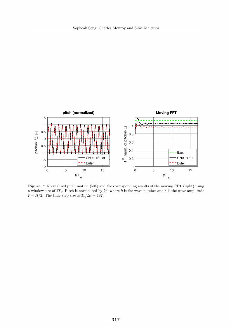
When using the Euler scheme the seakeeping simulations run stable for more than 17Te.The 2D wave propagation tests show clearly that the Euler scheme is not appropriated sincewaves are decaying significantly from FP to AP. The 3D seakeeping mesh has the similar meshconfiguration as in 2D and all relevant numerical schemes as well as the time step are kept thesame between 2D and 3D simulations. Hence it is expected that the resulting incident waveswhen using the Euler scheme in 3D have the same decay rate as seen on the 2D mesh. Wheninspecting the resulting heave and pitch motions, however, it is not clear how the conditionwhere waves at FP and AP may have different amplitudes affects the heave and pitch motions.Figures 6 and 7 show results of a moving FFT on heave and pitch motions. Since the simulatedincident waves are decaying and therefore have some loss of amplitude the resulting heave andpitch motions are reduced accordingly. The resulting ship motions are expected to be improvedwhen using the CrankNicolson scheme.

With CrankNicolson 0.9 the 2D wave simulation on the 2D mesh is stable. However, the3D seakeeping mesh has small irregular cells which are produced in the process of cutting andfitting the mesh to the ship hull. These irregular cells are expected to have a negative influenceon the overall numerical stability. Furthermore the presence of the ship hull and its motioninduces a larger local flow in the vicinity of the hull which causes the local Courant number to

10

914


Figure 5: Cells next to the ship hull at a distance of less than 0.0245 m (shaded area) are selected foruse with co = 0 (i.e. the same as the Euler scheme). All other cells not included in this selection areintegrated using co = 0.9. Close-up view at stern (left), at bow (right).

increase. It is our discovery that the 3D seakeeping simulation at co = 0.9 becomes unstablevery quickly. Once again the stability can be restored by reducing the value of co further toward0 (i.e. the Euler scheme) and at same time decrease the time step (see Fig. 4) considerablyto maintain an acceptable accuracy of wave simulations. In the current 3D seakeeping casewe are exploring a more efficient solution by reducing co not globally but in locally selectedcells where the local Courant numbers either are considered too large or have poor geometricalproperties. The selection is done based on authors own intuition and convenience rather thanon a rigorous optimization. Figure 5 illustrates these local cells (shaded region). The selectionis done manually prior to each run using cell selection tools available in OpenFOAM. Here adistance based cell selection tool has been used to selected all cells within a normal distance of0.0245 m to the ship hull. This short distance covers a few layers of cells which, in some regions,can be very small. The simulation is performed using CrankNicolson 0.9 in all cells exceptthose selected for used with CrankNicolson 0 (i.e. equivalent to the implicit backward Euler

scheme, see also Eq. (7)). With this selection the off-centering coefficient co changes abruptlyfrom 0.9 to 0. While it is possible to distribute the co values more smoothly no such attempthas been made since the current selection is already very stable. The seakeeping simulationsrun for more than 17Te. The resulting heave and pitch motions are shown in Fig. 6 and 7with label CN0.9+Euler. The time series of heave and pitch motions are processed in to thefrequency domain using a moving FFT with a window size of 1Te. The evolution of the 1st

harmonic confirms that the resulting motions have reached a quasi-steady state in less than17Te. More importantly the predicted amplitude of the 1st harmonics (for both heave andpitch) are significantly closer to the experiments. Some small variations still exist, possibly dueto disturbance produced by a non-perfect wave treatments at the outlet boundaries. Table 3shows a comparison of the amplitudes of the 1st harmonics between the current simulations andother CFD codes reported in [12]. Using the experiments as a reference for the comparison it isevident that the CN0.9+Euler scheme is superior than the Euler scheme. With respect to resultsfrom other CFD codes the percentage errors in the present simulations using CN0.9+Euler areapproximately at the same level as reported by UNIZAG-FSB/swenseFoam and FORCE/StarCCM+.While these results are very encouraging for a further study of the CN0.9+Euler scheme it shallbe stressed that the use of the CN0.9+Euler scheme combination is not strictly unambiguous

11

915


0 5 10 15

-1.5

-1

-0.5

0

0.5

1

t/T e

heav

e/ξ,

[-]

heave (normalized)

CN0.9+EulerEuler

0 5 10 150

0.2

0.4

0.6

0.8

1

t/T e

1stha

rm. o

f hea

ve/ξ

Moving FFT

Exp.CN0.9+EulEuler

Figure 6: Normalized heave motion (left) and the corresponding results of the moving FFT (right)using a window size of 1Te. Heave is normalized by wave amplitude ξ = H/2. The time step size isTe/∆t ≈ 187.

due to the uncertainty on how to select properly the distribution of co. Moreover there are othertemporal schemes which may perhaps produce results at least at a similar level of accuracyand performance without introducing ambiguous parameters as with the CN0.9+Euler scheme.The major barrier in OpenFOAM, however, is that MULES which is the dominating solverfor the transport equation of the phase fraction field currently only supports the Euler andCrankNicolson schemes for the reasons that these two schemes can keep the α-field boundedbetween 0 and 1.

5 CONCLUSIONS

The results of the 2D wave propagation tests and the 3D seakeeping tests show that Open-FOAM has the capacity to simulate regular head wave conditions reasonably well. Since the testcondition presented in this paper only covers one wave condition there is a need for more testson a larger variety of wave and test conditions in order to draw a firm conclusion on whetheror not OpenFOAM can be applied satisfactory in a practical engineering application. Alreadythe results presented here reveal some weaknesses and limitations related to the stability ofthe available 2nd-order CrankNicolson scheme and the accuracy of wave probing tools. Themodified CrankNicolson scheme provides a better accuracy at an increasing value of co, Fig.4. When co is too large, however, the simulation may become unstable. Here it is shown thatthe stability can be restored by reducing co value only at local regions where the cell qualityor the flow are considered critical. Without reducing the co value globally waves are allowedto propagate more accurately toward the ship which helps to improve significantly the overallaccuracy of the predicted ship motions.

12

916


0 5 10 15-2

-1.5

-1

-0.5

0

0.5

1

1.5

t/T e

pitch

/(kξ)

, [-]

pitch (normalized)

CN0.9+EulerEuler

0 5 10 150

0.2

0.4

0.6

0.8

1

t/T e

1stha

rm. o

f pitc

h/(k

ξ)

Moving FFT

Exp.CN0.9+EulEuler

Figure 7: Normalized pitch motion (left) and the corresponding results of the moving FFT (right) usinga window size of 1Te. Pitch is normalized by kξ, where k is the wave number and ξ is the wave amplitudeξ = H/2. The time step size is Te/∆t ≈ 187.

13

917


Table 1: The seakeeping case used in this work c.f. [12]. Wave crest is at FP at t = 0 s. Heave motionnormalized by wave amplitude ξ = H/2, pitch angle by kξ, forces by 0.5ρU2S0. Sinkage is positiveupwards. Trim is positive bow up.

Hull data (model scale)KCS Model 2, Case-2.10

Length btw. perpendiculars, Lpp, [m] 6.0702Maximum beam of waterline, B [m] 0.8498Draft, [m] 0.2850Displacement volume, [m3] 0.9571LCB, [%Lpp, fwd+] -1.4800Vert. CoG, [m, from keel] 0.3780Moment of Inertia, [Kxx/B] 0.4000Moment of Inertia, [Kyy/Lpp, Kzz/Lpp] 0.2520

Test condition(Towed in regular head wave)

Degree-of-freedom, heave & pitchTowing speed, [m/s] 2.0170Wave length, λ [m] 11.840Wave height, H [m] 0.1960Froude number, Fr 0.2610Reynolds number, Re 1.074 · 107Water depth, d [m] 5.5

Derived wave propertiesbased on [5]

Period, T [s] 2.7581Wave frequency, ω [rad/s] 2.2781Encounter frequency, ωe [rad/s] 3.3484Wave number, k [1/m] 0.5307kd [-] 2.9186H/λ [-] 0.0165Phase velocity, c [m/s] 4.2929

Experimental results c.f. [12]ampl. (0th, 1st, 2nd, 3rd, 4th)phase (1st, 2nd, 3rd, 4th)

Wave, ampl. [/Lpp] 1st-harm. 0.01611Thrust Coeff., CT, ampl. [103], phase [rad]ampl. (10.842, 25.101, 0.655, 0.581, 0.595)phase (-0.3585, 0.0890, 1.5306, -0.8437)Heave, ampl. [/ξ], phase [rad]ampl. (-0.2005, 0.9312, 0.0206, 0.0013, 0.0002)phase (-1.7205, 1.3007, 1.6636, 0.5488)Pitch, ampl. [/(kξ)], phase [rad]ampl. (-0.0562, 1.1185, 0.0379, 0.0017, 0.0003)phase (-0.5811, 2.1387, 0.8706, -0.3979)

14

918


Table 2: The description of the FVM schemes used in this work

FVM SchemeDescription

(name in OpenFOAM)

Euler 1st-order implicit backward Euler schemeCrankNicolson co Modified Crank-Nicolson with off-center coefficient cobackward 2nd-order three-time-steps backward differencing schemevanLeer01 2nd-order scheme with van Leer’s limiter bounded between [0, 1]interfaceCompression High-resolution scheme for the artificial compression termlinear 2nd-order central differencing scheme (linear interpolation)linear correct Linear interpolation with explicit non-orthogonal correctionlinearUpwind 2nd-order upwind scheme

Spatial/interpolation schemes used in all simulations

Divergence operator ∇ · (αu) vanLeer01

∇ · [α(1− α)ur] interfaceCompression

∇ · (ρu)uT linearUpwind

Laplacian operator linear corrected

Gradient operator linear

Cell-to-face interpolation linear

Table 3: Amplitudes of the 1st harmonic of normalized heave (z/ξ) and pitch (θ/(kξ)) motions c.f. [12].The experimental data (EFD) is from the towing tests performed at FORCE Technology. The errorsin percent are computed as 100(S − EFD)/EFD, where S are the simulated results and EFD are theexperiments.

KCS CASE 2.10-C5 heave, z/ξ Err. [%] pitch, θ/(kξ) Err. [%]

EFD 0.9312 - 1.1185 -

Present Simulations/CN0.9+Euler 0.866 -7.00 1.050 -6.12Present Simulations/Euler 0.808 -13.23 0.962 -13.99FORCE/StarCCM+ 0.874 -6.14 1.084 -3.08HSVA/FreSCO+ 0.899 -3.46 1.087 -2.81IIHR/CFDShip-Iowa v.4.5 0.917 -1.52 1.090 -2.55KRISO/WAVIS 0.741 -20.43 0.886 -20.79MARIC/FINEMarine313 0.944 1.37 1.163 3.98NMRI/NAGISA 0.925 -0.67 1.047 -6.39NUMECA/ISISCFD 0.898 -3.57 1.080 -3.44UM/OF23x 0.901 -3.24 1.078 -3.62UNIZAG-FSB/swenseFoam, Grid#1 0.876 -5.93 1.038 -7.20

15

919


REFERENCES

[1] The OpenFOAM Foundation Ltd, www.openfoam.org

[2] Weller, H.G.; Tabor, G.; Jasak, H. and Fureby, C.: A Tensorial Approach to ComputationalContinuum Mechanics using Object Orientated Techniques. J. Comput. Phys. 12, 6 (Nov.1998) 620–631. (doi:10.1063/1.168744)

[3] Jacobsen, N. G.; Fuhrman, D. R. and Fredse, J.: A wave generation toolbox for theopen-source CFD library: OpenFoam. Int. J. Numer. Meth. Fluids (2012), 70:1073–1088.doi:10.1002/fld.2726

[4] Monroy, C.; Seng, S. and Malenica, S.: Developpements et validation de l’outil CFD Open-FOAM pour le calcul de tenue a la mer. 15 emes Journees de l’Hydrodynamique, (22-24Nov. 2016), Brest.

[5] Fenton, J. D.: The numerical solution of steady water wave problems. Computers &Geosciences 14, 3 (1988), 357–368, ISSN 0098–3004, http://dx.doi.org/10.1016/0098-3004(88)90066-0.

[6] Hirt, C.W and Nichols, B.D.: Volume of fluid (VOF) method for the dynamics of freeboundaries. J. Comput. Phys. 39, 1 (Jan. 1981), 201–225.

[7] Issa, R. I.: Solution of the implicitly discretised fluid flow equations by operator-splitting. J. Comput. Phys. 62, 1 (Jan. 1986), 40-65. DOI=10.1016/0021-9991(86)90099-9http://dx.doi.org/10.1016/0021-9991(86)90099-9

[8] Damian, S. M.: An Extended Mixture Model for the Simultaneous Treatment of Short andLong Scale Interfaces. PhD thesis, Universidad Nacional del Litoral, Santa Fe, Argentina,(2013)

[9] Deshpande, S. S; Anumolu, L. and Trujillo, M. F .: Evaluating the performance of thetwo-phase flow solver interFoam. Comput. Sci. Disc. (2012) 5 014016

[10] Seng, S.; Pedersen, P. T. (Supervisor) and Jensen, J. J. (Supervisor).: Slamming And Whip-ping Analysis Of Ships. PhD thesis, Technical University of Denmark, Lyngby, Denmark,(2012)

[11] Simonsen, C.; Otzen, J. and Stern, F.: EFD and CFD for KCS heaving and pitching inregular head waves. In Proc. 27th Symp. Naval Hydrodynamics, Seoul, Korea, 2008.

[12] Tokyo 2015: A Workshop on CFD in Ship Hydrodynamics, Dec. 2-4, 2015,www.t2015.nmri.go.jp

16

920

on the use of euler and crank-nicolson time-stepping

Documents