a crank--nicolson adi spectral method for a two ...eprints.qut.edu.au/82655/8/82655_pubver.pdf ·...

Copyright © by SIAM. Unauthorized reproduction of this article is prohibited.

SIAM J. NUMER. ANAL. c© 2014 Society for Industrial and Applied MathematicsVol. 52, No. 6, pp. 2599–2622

A CRANK–NICOLSON ADI SPECTRAL METHOD FOR ATWO-DIMENSIONAL RIESZ SPACE FRACTIONAL NONLINEAR

REACTION-DIFFUSION EQUATION∗

FANHAI ZENG† , FAWANG LIU‡ , CHANGPIN LI§ , KEVIN BURRAGE¶, IAN TURNER‡ ,AND V. ANH‡

Abstract. In this paper, a new alternating direction implicit Galerkin–Legendre spectral methodfor the two-dimensional Riesz space fractional nonlinear reaction-diffusion equation is developed. Thetemporal component is discretized by the Crank–Nicolson method. The detailed implementation ofthe method is presented. The stability and convergence analysis is strictly proven, which shows thatthe derived method is stable and convergent of order 2 in time. An optimal error estimate in spaceis also obtained by introducing a new orthogonal projector. The present method is extended to solvethe fractional FitzHugh–Nagumo model. Numerical results are provided to verify the theoreticalanalysis.

Key words. alternating direction implicit method, Legendre spectral method, Riesz spacefractional reaction-diffusion equation, fractional FitzHugh–Nagumo model, stability and convergence

AMS subject classifications. 26A33, 65M06, 65M12, 65M15, 35R11

DOI. 10.1137/130934192

1. Introduction. In the past decades, fractional calculus has been used to modelparticle transport in porous media. Recently, there has been increasing interest in thestudy of fractional calculus for its wide application in many fields of science andengineering, such as the physical and chemical processes, materials, control theory,biology, finance, and so on (see [3, 9, 25, 23, 33, 35]). In physics, fractional derivativesare used to model anomalous diffusion, where particles spread differently than theclassical Brownian motion model [23]. Kinetic equations of the diffusion, diffusion-advection, and Fokker–Planck equations with partial fractional derivatives were rec-ognized as a useful approach for the description of transport dynamics in complexsystems. Reaction-diffusion models have been used for numerous applications in pat-ten formation in biology, chemistry, physics, and engineering. These systems showthat diffusion can produce the spontaneous formation of spatial-temporal patterns.The idea is to use a fractional-order density gradient to recover, at least at a phe-nomenological level, the nonhomogeneities of the porous media. Given the structural

∗Received by the editors August 23, 2013; accepted for publication (in revised form) June 5,2014; published electronically November 4, 2014. This work was supported by the National NaturalScience Foundation of China (grant 11372170), a grant of “The First-class Discipline of Universityin Shanghai,” the Key Program of Shanghai Municipal Education Commission (grant 12ZZ084), andthe Australian Research Council (grant DP120103770). This work was also supported by the ChinaScholarship Council (CSC).

http://www.siam.org/journals/sinum/52-6/93419.html†Department of Mathematics, Shanghai University, Shanghai 200444, People’s Republic of China,

and Department of Mathematics, Tongji University, Shanghai 200092, People’s Republic of China([email protected]).

‡School of Mathematical Sciences, Queensland University of Technology, GPO Box 2434, Bris-bane, Queensland 4001, Australia ([email protected], [email protected], [email protected]).

§Department of Mathematics, Shanghai University, Shanghai 200444, People’s Republic of China([email protected]).

¶School of Mathematical Sciences, Queensland University of Technology, GPO Box 2434, Bris-bane, Queensland 4001, Australia, and Department of Computer Science, OCISB, University ofOxford, OXI 3QD, UK ([email protected]).

2599

Dow

nloa

ded

03/2

2/15

to 1

31.1

81.2

51.1

30. R

edis

trib

utio

n su

bjec

t to

SIA

M li

cens

e or

cop

yrig

ht; s

ee h

ttp://

ww

w.s

iam

.org

/jour

nals

/ojs

a.ph

p

http://www.siam.org/journals/sinum/52-6/93419.html

mailto:[email protected]







2600 ZENG, LIU, LI, BURRAGE, TURNER, AND ANH

analogy between Newton’s law of viscosity and Fick’s law of particles transport, theusage of a fractional Newton’s law for descripting momentum transport in nonho-mogeneous porous media could be considered. By using spatial averaging meth-ods, Ochoa-Tapia, Valdes-Parada, and Alvarez-Ramirez [32] derived a Darcy-typelaw from a fractional Newton’s law of viscosity, which is intended to describe shearstress phenomena in nonhomogeneous porous media. Valdes-Parada, Ochoa-Tapia,and Alvarez-Ramirez [39] studied reaction-diffusion phenomena in disordered porousmedia with non-Fickian diffusion effects. They obtained an effective medium equationof the concentration dynamics, which has a fractional Fick’s law for the particles flux.They showed that the macroscale diffusion parameter is affected by the scaling frommesoscale to macroscale, and by the disordered structure of the porous medium.

In this paper, we consider the following two-dimensional Riesz space fractionalnonlinear reaction-diffusion equation [3, 19]:(1.1)⎧⎪⎪⎪⎨⎪⎪⎪⎩

∂tu = Kx∂2α1u

∂|x|2α1+Ky

∂2α2u

∂|y|2α2+ F (u) + f(x, y, t), (x, y, t)∈Ω×(0, T ], T > 0,

u(x, y, 0) = φ0(x, y), (x, y)∈Ω,

u = 0, (x, y, t)∈ ∂Ω× (0, T ],

in which 12 < α1, α2 < 1, Kx,Ky > 0, Ω = (a, b) × (c, d), ∂t =

∂∂t . F (u) is nonlinear,

which satisfies the requirement that |∂uF (u)| is bounded when u is bounded or F (u)

satisfies the local Lipschitz condition, and ∂2α1

∂|x|2α1and ∂2α2

∂|y|2α2are the Riesz fractional

operators [9, 33, 36] defined by

∂2α1u

∂|x|2α1= −c1(RLD

2α1a,x u+RL D2α1

x,b u),

∂2α2u

∂|y|2α2= −c2(RLD

2α2c,y u+ RLD

2α2

y,d u),

where c1 = 12 cos(α1π)

, c2 = 12 cos(α2π)

. For n− 1 < β < n, n∈N, the operators RLDβa,x,

RLDβx,b, RLD

βc,y, and RLD

βy,d are defined as

RLDβa,xu =

∂n

∂xn

[D−(n−β)

a,x u]=

1

Γ(n− β)

∂n

∂xn

∫ x

a

(x− s)n−β−1u(s, y, t) ds,

RLDβx,bu = (−1)n

∂n

∂xn

[D

−(n−β)x,b u

]=

(−1)n

Γ(n− β)

∂n

∂xn

∫ b

x

(s− x)n−β−1u(s, y, t) ds,

RLDβc,yu =

∂n

∂yn

[D−(n−β)

c,y u]=

1

Γ(n− β)

∂n

∂yn

∫ y

c

(y − s)n−β−1u(x, s, t) ds,

RLDβy,du = (−1)n

∂n

∂yn

[D

−(n−β)y,d u

]=

(−1)n

Γ(n− β)

∂n

∂yn

∫ d

y

(s− y)n−β−1u(x, s, t) ds,

where D−μa,x and D−μ

x,b are the left and right Riemann–Liouville integral operatorsdefined by

D−μa,xu = RLD

−μa,xu =

1

Γ(μ)

∫ x

a

(x − s)μ−1u(s, y, t) ds, μ > 0,

D−μx,bu = RLD

−μa,xu =

1

Γ(μ)

∫ b

x

(s− x)μ−1u(s, y, t) ds, μ > 0.

Dow

nloa

ded

03/2

2/15

to 1

31.1

81.2

51.1

30. R

edis

trib

utio

n su

bjec

t to

SIA

M li

cens

e or

cop

yrig

ht; s

ee h

ttp://

ww

w.s

iam

.org

/jour

nals

/ojs

a.ph

p


CNADIGLS FOR TWO-DIMENSIONAL RSFDE 2601

The left and right Riemann–Liouville integral operators D−μc,y and D−μ

y,d can be definedsimilarly.

There are several analytical techniques to solve fractional differential equations(FDEs), such as the Fourier transform method, the Laplace transform method, theMellin transform method, and the Green function method [23, 33]. Anh and Leo-nenko [1] presented a spectral representation of the mean-square solution of the frac-tional kinetic equation with random initial condition. The explicit strong solutionsfor fractional Pearson diffusions are developed by using spectral methods involvingthe Mittag–Leffler function in [10]. In most situations, analytical methods do notwork well on most FDEs, so the reasonable option is to resort to numerical methods.Up to now, there has been some work on numerical methods for FDEs, such as finitedifference methods [12, 20, 26, 47], finite element methods [5, 6, 11, 14, 42], spectralmethods [13, 15, 16], and so on [28, 29, 30]. Numerical methods for FDEs mainlyfocus on the linear equations; relatively few works have been developed for the non-linear FDEs. Until now, there have existed limited studies for nonlinear FDEs; see,for instance, [3, 6, 14, 17, 21, 48]. Very recently, Liu et al. [19] proposed an alternatingdirection implicit finite difference method to solve (1.1) with first-order in space.

In this paper, a Crank–Nicolson type alternating direction implicit Galerkin–Legendre spectral (CNADIGLS) method is developed to solve the two-dimensionalRiesz space fractional nonlinear reaction-diffusion equation, in which the temporalcomponent is discretized by the Crank–Nicolson method. The stability and conver-gence are strictly proven, which shows that the CNADIGLS method is conditionallystable and convergent with second-order accuracy in time, and the optimal error es-timate in space is derived by introducing a new orthogonal projector. In the stabilityanalysis, the nonlinear function F (u) satisfies the local Lipschitz condition or |∂uF (u)|is bounded in a suitable domain, which is a weaker condition compared with someexisting work [17, 21, 48]. The CNADIGLS method is extended to solve the frac-tional FitzHugh–Nagumo monodomain model. Numerical experiments are providedto verify the theoretical results, which are in good agreement with the theoreticalanalysis.

The remainder of this paper is organized as follows. Section 2 gives some notationand lemmas. In section 3, the CNADIGLS method is provided, and the implementa-tion of the CNADIGLS method is also presented in detail. The stability and conver-gence analysis is proven in section 4. In section 5, the derived method is extended tosolve the two-dimensional fractional FitzHugh–Nagumo model. The numerical resultsare presented in section 6, and the conclusion is given in the last section.

2. Preliminaries. In this section, we introduce some notation and lemmas thatare needed in the following sections.

Let Ω be a finite domain satisfying Ω = Ix×Iy = (a, b)×(c, d), and denote by (·, ·)the inner product on the space L2(Ω) with the L2 norm ‖ · ‖L2(Ω) and the maximumnorm ‖ · ‖L∞(Ω). We also define (·, ·) as the inner product on the interval Ix or Iy ifit does not cause confusion. Let μ be a nonnegative real number. We use Hμ(Ω) andHμ

0 (Ω) as the usual Sobolev spaces with the norm ‖ · ‖Hμ(Ω) and seminorm | · |Hμ(Ω)

(see [31, 35]). Denote by PN (Θ) the space of polynomials defined on the domain Θwith the degree no greater than N ∈Z+. The approximation space V 0

N is defined as

V 0N = (PN (Ix)⊗PN (Iy)) ∩H1

0 (Ω).

We introduce the Legendre–Gauss–Lobatto (LGL) interpolation operator IN :

Dow

nloa

ded

03/2

2/15

to 1

31.1

81.2

51.1

30. R

edis

trib

utio

n su

bjec

t to

SIA

M li

cens

e or

cop

yrig

ht; s

ee h

ttp://

ww

w.s

iam

.org

/jour

nals

/ojs

a.ph

p



C(Ω)→VN as

INu(xk, yl) = u(xk, yl), k, l = 0, 1, . . . , N,

where xk and yl are LGL points on the intervals Ix and Iy, respectively.Next, we introduce some spaces that are used in the formulation of the numerical

algorithms. We first introduce the spaces JμL(Ω), J

μR(Ω), and Jμ

S (Ω) in R2 (see [7]).

Definition 2.1. Let μ > 0. Define the seminorm

|u|JμL(Ω) =

(‖RLD

μa,xu(x, y)‖2L2(Ω) + ‖RLD

μc,yu(x, y)‖2L2(Ω)

)1/2and the norm

‖u‖JμL(Ω) =

(‖u‖2L2(Ω) + |u|2Jμ

L(Ω)

)1/2,

and denote JμL(Ω) (or Jμ

L,0(Ω)) as the closure of C∞(Ω) (or C∞0 (Ω)) with respect to

‖ · ‖JμL(Ω), where C∞

0 (Ω) is the space of smooth functions with compact support in Ω.Definition 2.2. Let μ > 0. Define the seminorm

|u|JμR(Ω) =

(‖RLD

μx,bu(x, y)‖2L2(Ω) + ‖RLD

μy,du(x, y)‖2L2(Ω)

)1/2and the norm

‖u‖JμR(Ω) =

(‖u‖2L2(Ω) + |u|2Jμ

R(Ω)

)1/2,

and denote JμR(Ω) (or Jμ

R,0(Ω)) as the closure of C∞(Ω) (or C∞0 (Ω)) with respect to

‖ · ‖JμR(Ω).Definition 2.3. Let μ �=n− 1/2, n∈N. Define the seminorm

|u|JμS (Ω) =

(|(RLD

μa,xu(x, y),RLD

μx,bu(x, y))|+ |(RLD

μc,yu(x, y),RLD

μy,du(x, y))|

)1/2and the norm

‖u‖JμS(Ω) =

(‖u‖2L2(Ω) + |u|Jμ

S (Ω)

)1/2,

and let JμS (Ω) (or Jμ

S,0(Ω)) denote the closure of C∞(Ω) (or C∞0 (Ω)) with respect to

‖ · ‖JμS (Ω).The fractional Sobolev space Hμ(Ω) can be defined via the Fourier transform

approach.Definition 2.4 (see [31, 35]). Let μ > 0. Define the seminorm

|u|Hμ(Ω) = ‖ |ω|μF(u)(ω) ‖L2(R2)

and the norm

‖u‖Hμ(Ω) =(‖u‖2L2(Ω) + |u|2Hμ(Ω)

)1/2,

where F(u)(ω) is the Fourier transformation of function u(x, y). And let Hμ(Ω) (orHμ

0 (Ω)) be the closure of C∞(Ω) (or C∞0 (Ω)) with respect to ‖ · ‖Hμ(Ω).

Lemma 2.5 (see [35]). Let μ > 0, Ω = (a, b)× (c, d), u∈JμL,0(Ω)∩Jμ

R,0(Ω). Then

(RLDμa,xu,RLD

μx,bu) = cos(μπ)‖RLD

μ−∞,xu‖2L2(R2) = cos(μπ)‖RLD

μx,∞u‖2L2(R2),

(RLDμc,yu,RLD

μy,du) = cos(μπ)‖RLD

μ−∞,yu‖2L2(R2) = cos(μπ)‖RLD

μy,∞u‖2L2(R2),

Dow

nloa

ded

03/2

2/15

to 1

31.1

81.2

51.1

30. R

edis

trib

utio

n su

bjec

t to

SIA

M li

cens

e or

cop

yrig

ht; s

ee h

ttp://

ww

w.s

iam

.org

/jour

nals

/ojs

a.ph

p



where u is the extension of u by zero outside Ω. Furthermore, if μ �=n−1/2, n∈N, andu∈Jμ

L,0(Ω), then there exists a positive constant C independent of u such that

|u|JμL(R2) ≤C|u|Jμ

L(Ω).

Lemma 2.6. Let μ1, μ2 > 0, Ω = (a, b)×(c, d), u∈Jmax{μ1,μ2}L,0 (Ω)∩Jmax{μ1,μ2}

R,0 (Ω).Then

(RLDμ1a,xRLD

μ2c,yu,RLD

μ1

x,bRLDμ2

y,du) = cos(μ1π) cos(μ2π)‖RLDμ1

−∞,xRLDμ2

−∞,yu‖2L2(R2),

(RLDμ1a,xRLD

μ2

y,du,RLDμ1

x,bRLDμ2c,yu) = cos(μ1π) cos(μ2π)‖RLD

μ1

−∞,xRLDμ2

−∞,yu‖2L2(R2),

where u is the extension of u by zero outside Ω.Proof. The proof is similar to Lemma 3.1.4 in [35], we omit the details here. The

proof is completed.Lemma 2.7 (see [7]). Let Ω = (a, b)×(c, d), μ �=n− 1

2 , n∈N, and u∈JμL,0(Ω)∩Jμ

R,0(Ω)

∩Hμ0 (Ω). Then there exist positive constants C1 and C2 independent of u such that

C1|u|Hμ(Ω) ≤ max{|u|Jμ

L(Ω), |u|JμR(Ω)

}≤C2|u|Hμ(Ω).(2.1)

Remark 2.1. In fact, the spaces JμL,0(Ω), J

μR,0(Ω), J

μS,0(Ω), and Hμ

0 (Ω) are equiv-alent, with equivalent seminorms and norms if μ �=n − 1/2, n∈N; see [7] for moredetails.

Lemma 2.8 (see [7]). Let 1 < β < 2. Then for any u∈Hβ0 (Ω) and v ∈H

β/20 (Ω),

we have

(RLDβa,xu, v) = (RLD

β/2a,x u,RLD

β/2x,b v), (RLD

βx,bu, v) = (RLD

β/2x,b u,RLD

β/2a,x v).

3. The scheme and implementation. In this section, we first present theCrank–Nicolson type ADI Legendre spectral method for (1.1). Then, we give thedetailed implementation of the proposed method.

Let τ be the time step size and nT be a positive integer with τ = T/nT andtn = nτ for n = 0, 1, . . . , nT . Denote tn+1/2 = (tn + tn+1)/2 for n = 0, 1, . . . , nT − 1.For the function u(x, y, t)∈C(Ω× [0, T ]), denote un = un(·) = u(·, tn). For simplicity,we introduce the following notation:

δtun+1/2 =

un+1 − un

τ, un+1/2 =

un+1 + un

2.

3.1. The fully discrete scheme. In this subsection, we present the fully dis-crete scheme for (1.1). We first give a simple description of the time discretization of

(1.1). Let Lxu = Kx∂2α1u∂|x|2α1

and Lyu = Ky∂2α2u∂|y|2α2

. Then (1.1) can be rewritten as

(3.1) ∂tu = (Lx + Ly)u+ F (u) + f(x, y, t).

Suppose that u(x, y, t) is sufficiently smooth with respect to time. At each time leveln, the temporal derivative of (3.1) is discretized by the Crank–Nicolson method, i.e.,∂tu(tn+1/2) = δtu

n+1/2 +O(τ2) and (Lx + Ly)u(tn+1/2) = (Lx + Ly)un+1/2 +O(τ2),

which yields

(3.2) δtun+1/2 = (Lx + Ly)u

n+1/2 +1

2(F (un+1) + F (un)) + f(tn+1/2) +O(τ2).

Dow

nloa

ded

03/2

2/15

to 1

31.1

81.2

51.1

30. R

edis

trib

utio

n su

bjec

t to

SIA

M li

cens

e or

cop

yrig

ht; s

ee h

ttp://

ww

w.s

iam

.org

/jour

nals

/ojs

a.ph

p



Adding the perturbation term τ2

4 LxLyδtun+1/2 = O(τ2) to the left side of (3.2) gives

(3.3)δtu

n+1/2 +τ2

4LxLyδtu

n+1/2 = (Lx + Ly)un+1/2

+1

2(F (un+1) + F (un)) + f(tn+1/2) +O(τ2).

One can also rewrite (3.3) into the following equivalent form:

(3.4)

(1− τ

2Lx

)(1− τ

2Ly

)un+1 =

(1 +

τ

2Lx

)(1 +

τ

2Ly

)un−1

+τ

2(F (un+1) + F (un)) + τf(tn+1/2) +O(τ3).

From (3.4), we can obtain the fully discrete CNADIGLS method for (1.1) asfollows: Find un+1

N ∈V 0N for n = 0, 1, . . . , nT − 1 such that

(3.5)

⎧⎪⎪⎪⎨⎪⎪⎪⎩

((1− τ

2Lx

)(1− τ

2Ly

)un+1N , v

)=((

1 +τ

2Lx

)(1 +

τ

2Ly

)unN , v

)+

τ

2(INF (un+1

N ) + INF (unN), v) + τ(INf(tn+1/2), v) ∀v ∈V 0

N ,

u0N = Π1,0

N φ0,

where Π1,0N is an appropriate projection operator; see also Lemma 4.3 in section 4.

3.2. Implementation of the CNADIGLS method. In this subsection, wegive a detailed description of the implementation of the CNADIGLS method (3.5).As in [38], the function spaces V x,0

N and V y,0N can be expressed as

V x,0N = span {φl(x) : l = 0, 1, . . . , N − 2} ,

V y,0N = span {ϕl(y) : l = 0, 1, . . . , N − 2} ,

in which φl(x) and ϕl(y) are defined as in [38]:

(3.6)φl(x) = Ll(x)− Ll+2(x), x∈ [−1, 1], x =

(b− a)x+ a+ b

2∈ [a, b],

ϕl(y) = Ll(y)− Ll+2(y), y ∈ [−1, 1], y =(d− c)y + c+ d

2∈ [c, d],

where Ll(z) (z ∈ [−1, 1], l ∈ Z+) is the Legendre polynomial defined by the followingrecurrence relation [37]:

(3.7) L0(z) = 1, L1(z) = z, Ll+1(z) =2l+ 1

l + 1zLl(z)− l

l + 1Ll−1(z), l ≥ 1.

The Jacobi polynomials P a,bl (z) (a, b > −1, z ∈ [−1, 1], l ∈ Z+) are orthogonal

with respect to the weight function ωa,b(z) = (1− z)a(1 + z)b; these polynomials areused in the numerical computation. The explicit formula of the Jacobi polynomial isstated as follows [37]:

(3.8) P a,bl (z) = 2−l

l∑j=0

(l+ a

j

)(l + b

l− j

)(z − 1)l−j(z + 1)j .

Dow

nloa

ded

03/2

2/15

to 1

31.1

81.2

51.1

30. R

edis

trib

utio

n su

bjec

t to

SIA

M li

cens

e or

cop

yrig

ht; s

ee h

ttp://

ww

w.s

iam

.org

/jour

nals

/ojs

a.ph

p



The Jacobi polynomials can also be generated by the three-term recurrence formula;see [4, 37] for more details.

Therefore, the function space V 0N = V x,0

N ⊗ V y,0N can be given by

V 0N = span

{φk(x)ϕl(y), k, l = 0, 1, . . . , N − 2

}.

Next, we give the matrix representation of the CNADIGLS method (3.5). Theunknown function un+1

N ∈ V 0N has the following form:

(3.9) un+1N =

N−2∑k=0

N−2∑l=0

cn+1k,l φk(x)ϕl(y).

Set the matrices Mx,My, Sx, Sy ∈R(N−1)×(N−1) that satisfy

(Mx)k,l = (φk, φl), (Sx)k,l = (RLDα1

x,bφk,RLDα1a,xφl),

(My)k,l = (ϕk, ϕl), (Sy)k,l = (RLDα2

y,dϕk,RLDα2c,yϕl).

Inserting un+1N into the CNADIGLS method (3.5) and letting v = φkϕl (k, l = 0, 1, . . . ,

N − 2), we obtain the matrix representation of the CNADIGLS method as follows:

(3.10)(Mx − τ

2c1Kx(Sx + ST

x ))Cn+1

(My − τ

2c2Ky(Sy + ST

y ))T

= RHSn +Nn+1,

where Cn+1, RHSn, Nn+1 ∈R(N−1)×(N−1), satisfying

(Cn+1)k,l = cn+1k,l , k, l = 0, 1, . . . , N − 2,

RHSn =(Mx +

τ

2c1Kx(Sx + ST

x ))Cn(My +

τ

2c2Ky(Sy + ST

y ))T

+ τGn,

(Gn)k,l = (INfn+1/2, φkϕl) +1

2(INF (un

N), φkϕl), k, l = 0, 1, . . . , N − 2,

Gn ∈R(N−1)×(N−1),

(Nn+1)k,l =τ

2(INF (un+1

N ), φkϕl), k, l = 0, 1, . . . , N − 2.

Let M1 = Mx − τ2 c1Kx(Sx + ST

x ), M2 = My +τ2 c2Ky(Sy + ST

y ). Then (3.10) canbe rewritten into the following form:

(3.11) M1Cn+1MT

2 = RHSn +Nn+1.

Noticing that Nn+1 = Nn+1(un+1N ), we can solve system (3.11) by the following

Dow

nloa

ded

03/2

2/15

to 1

31.1

81.2

51.1

30. R

edis

trib

utio

n su

bjec

t to

SIA

M li

cens

e or

cop

yrig

ht; s

ee h

ttp://

ww

w.s

iam

.org

/jour

nals

/ojs

a.ph

p



iteration algorithm:

Set Cn+1,0 = Cn, un+1,0N =

N−2∑k=0

N−2∑l=0

cn+1,0k,l φk(x)ϕl(y);

for m = 0 : K − 1

Solve M1C∗ = RHSn +Nn+1(un+1,m

N ) to obtain C∗;

Solve M2(Cn+1,m+1)T = (C∗)T to obtain Cn+1,m+1;

Compute un+1,m+1N =

N−2∑k=0

N−2∑l=0

cn+1,m+1k,l φk(x)ϕl(y);

If ‖un+1,m+1N − un+1,m

N ‖L∞(Ω) ≤ ε

break;

end if

end for

Set Cn+1 = Cn+1,m+1.

Here K is a suitable positive integer and ε is a suitably small positive constant.Obviously, we just need to solve an array of the algebraic systems of the form

Ax = b (A = M1,M2) to get the numerical solutions, which can be done in parallel.The coefficient matrices (i.e., M1 and M2) of the algebraic system derived from theCNADIGLS method have the same size as those of the coefficient matrix derived fromthe corresponding one-dimensional FPDE [19].

Computation of the matrices Sx and Sy. We give an illustration of cal-culating the matrices Sx and Sy. We mainly focus on the computation of Sx; thecomputation of Sy is almost the same as that of Sx. The matrices Mx and My canbe easily derived from the orthogonality of the Legendre polynomials [37], so we omitthe details.

Lemma 3.1 (see [37]). Suppose that

Pα,βn (x) =

n∑k=0

cnkPa,bk (x), a, b, α, β > −1,

where Pα,βn (x) is a Jacobi polynomial. Then

cnk =cnk (α, β) =Γ(n+ α+ 1)

Γ(n+ α+ β + 1)

(2k + a+ b+ 1)Γ(k + a+ b+ 1)

Γ(k + a+ 1)

×n−k∑m=0

(−1)mΓ(n+ k +m+ α+ β + 1)Γ(m+ k + a+ 1)

(n− k −m)!m!Γ(k +m+ α+ 1)Γ(m+ 2k + a+ b+ 1).

Lemma 3.2 (see [8]). For μ > 0, then

RLDμ−1,xLn(x) =

Γ(n+ 1)

Γ(n− μ+ 1)(1 + x)−μPμ,−μ

n (x), x ∈ [−1, 1],

RLDμx,1Ln(x) =

Γ(n+ 1)

Γ(n− μ+ 1)(1− x)−μP−μ,μ

n (x), x ∈ [−1, 1],

where Ln(x) is a Legendre polynomial and Pα,βn (x)(α, β > −1) is a Jacobi polynomial.

Dow

nloa

ded

03/2

2/15

to 1

31.1

81.2

51.1

30. R

edis

trib

utio

n su

bjec

t to

SIA

M li

cens

e or

cop

yrig

ht; s

ee h

ttp://

ww

w.s

iam

.org

/jour

nals

/ojs

a.ph

p



Since (RLDα1

x,bφk,RLDα1a,xφl) = (RLD

α1

x,b(Lk(x)−Lk+2(x)),RLDα1a,x(Ll(x)−Ll+2(x))),

we just need to calculate (RLDα1

x,bLk(x),RLDα1a,xLl(x)). It is easy to obtain

RLDα1a,xLk(x) =

1

Γ(1− α1)

d

dx

∫ x

a

(x− s)−α1Lk(s) ds =

(b− a

2

)−α1

RLDα1

−1,xLk(x),

RLDα1

x,bLk(x) =

(b − a

2

)−α1

RLDα1

x,1Lk(x),

where we have used the transforms x = (b−a)x+a+b2 ∈ [a, b] and s = (b−a)s+a+b

2 ∈ [a, b].

Hence, using Lemma 3.1 and the transform x = (b−a)x+a+b2 ∈ [a, b] once more, we have

(RLDα1a,xLk(x),RLD

α1

x,bLl(x)) =

∫ b

aRLD

α1a,xLk(x)RLD

α1

x,bLl(x) dx

=

(b− a

2

)1−2α1∫ 1

−1RLD

α1

−1,xLk(x)RLDα1

x,1Ll(x) dx

=

(b− a

2

)1−2α1 Γ(k + 1)

Γ(k − α1 + 1)

Γ(l + 1)

Γ(l − α1 + 1)

×∫ 1

−1

(1 + x)−α1(1 − x)−α1Pα1,−α1

k (x)P−α1,α1

l (x) dx.

We calculate the integral

I(k, l, α1) =

∫ 1

−1

(1 + x)−α1(1− x)−α1Pα1,−α1

k (x)P−α1,α1

l (x) dx

in two ways. We first give the exact expression of the above integral I(k, l, α1). ByLemma 3.1,

P−α1,α1n (x) =

n∑k=0

cnk (−α1, α1, )P−α1,−α1

k (x),

Pα1,−α1n (x) =

n∑k=0

cnk (α1,−α1, )P−α1,−α1

k (x).

By the orthogonality of Jacobi polynomials, one has

I(k, l, α1) =

min{l,k}∑r=0

clr(−α1, α1)ckr (α1,−α1)γ

−α1,−α1r ,

where

γ−α1,−α1r =

21−2α1(Γ(r − α1 + 1))2

(2r − 2α1 + 1)r!Γ(r − 2α1 + 1).

Next, we use the Gauss quadrature to calculate the integral I(k, l, α1), which readsas

(3.12) I(k, l, α1) ≈M∑j=0

ωjP−α1,α1

l (xj)Pα1,−α1

k (xj),

Dow

nloa

ded

03/2

2/15

to 1

31.1

81.2

51.1

30. R

edis

trib

utio

n su

bjec

t to

SIA

M li

cens

e or

cop

yrig

ht; s

ee h

ttp://

ww

w.s

iam

.org

/jour

nals

/ojs

a.ph

p



where {xj} are the Jacobi–Gauss–Lobatto points with respect to the weight functionω−α1,−α1(x) = (1+ x)−α1(1− x)−α1 . If M > N , then the numerical integration (3.12)is exact for all 0≤ k, l≤N . Of course, we can also choose Jacobi–Gauss or Jacobi–Guass–Radau quadrature to approximate the integral I(k, l, α1); see [37] for moredetails. In the numerical experiments, we use Jacobi–Gauss–Lobatto quadrature tocalculate the integral I(k, l, α1) for convenience.

4. Stability and convergence. In this section, we study the stability and con-vergence of the CNADIGLS scheme (3.5). We first introduce some notation andlemmas.

Denote

α = (α1, α2), αmax = max{α1, α2}, αmin = min{α1, α2},and

(4.1)A(u, v) =Kxc1

[(RLD

α1a,xu,RLD

α1

x,bv) + (RLDα1

x,bu,RLDα1a,xv)

]+Kyc2

[(RLD

α2c,yu,RLD

α2

y,dv) + (RLDα2

y,du,RLDα2c,yv)

].

Then the orthogonal projection operator Πα,0N : Hα1

0 ∩Hα20 (Ω) → V 0

N is defined as

(4.2) A(u −Πα,0N u, v) = 0, u ∈ Hα1

0 ∩Hα20 (Ω) ∀v ∈V 0

N .

For simplicity, we denote ‖ · ‖0 = ‖ · ‖ = ‖ · ‖L2(Ω) and ‖ · ‖∞ = ‖ · ‖L∞(Ω). Forα = (α1, α2), we define a new seminorm | · |α and norm ‖ · ‖α as

|u|α =(Kx‖RLD

α1a,xu‖2 +Ky‖RLD

α2c,yu)‖2

)1/2, ‖u‖α =

(‖u‖2 + |u|2α)1/2

.

From (4.1), we can easily obtain |u|α ≤C√

A(u, u).The seminorm |·|α and norm ‖·‖α are equivalent if u∈Hα1

0 ∩Hα20 (0 < α1, α2 ≤ 1),

which is given in the following lemma.Lemma 4.1. For u∈Hμ

0 (Ω) and 0 < s < μ, we have

(4.3) ‖u‖≤C1‖RLDsa,xu‖≤C2‖RLD

μa,xu‖, ‖u‖≤C3‖RLD

sc,yu‖≤C4‖RLD

μy,du‖,

where C1, C2, C3, and C4 are positive constants independent of u.Proof. See Theorem 3.1.9 and Corollary 3.1.10 in [35]. The proof is completed.Lemma 4.2. Suppose that Ω = (a, b)×(c, d), u∈Hα1

0 (Ω)∩Hα20 (Ω), 0 < α1, α2 ≤ 1.

Then there exists positive constants C1 < 1 and C2 independent of u, such that

(4.4) C1‖u‖α≤ |u|α≤‖u‖α≤C2|u|Hαmax (Ω).

Proof. The inequality |u|α ≤‖u‖α is obvious. By the definitions of | · |α and ‖ · ‖α,we need only prove that the inequality ‖u‖2≤ ( 1

C21− 1)|u|2α holds. From Lemma 4.1,

we have

|u|2α = Kx‖RLDα1a,xu‖2 +Ky‖RLD

α2c,yu‖2 ≤C(‖RLD

αmaxa,x u‖2 + ‖RLD

ααmaxc,y u‖2)

= C|u|2JmaxL (Ω).

Using the above inequality, Lemma 2.7, and the inequality ‖u‖α≤ 1C1

|u|α yields

‖u‖α≤ 1

C1|u|α≤

√C(C1)

−1|u|JαmaxL (Ω) ≤C2|u|Hαmax (Ω).

Dow

nloa

ded

03/2

2/15

to 1

31.1

81.2

51.1

30. R

edis

trib

utio

n su

bjec

t to

SIA

M li

cens

e or

cop

yrig

ht; s

ee h

ttp://

ww

w.s

iam

.org

/jour

nals

/ojs

a.ph

p



The proof is thus completed.Next, we introduce the properties of the projectors Π1,0

N and Πα,0N .

Lemma 4.3 (see [2]). Let s and r be real numbers satisfying 0≤ s≤ r. Then thereexist a projector Π1,0

N and a positive constant C depending only on r such that, forany function u∈Hs

0 (Ω)∩Hr(Ω), the following estimate holds:

‖u−Π1,0N u‖Hs(Ω) ≤CNs−r‖u‖Hr(Ω).

Lemma 4.4. Let αi, i = 1, 2 and r be arbitrary real numbers satisfying 0 < αi <1, αi < r, αi �= 1/2. Then there exists a positive constant C independent of N suchthat, for any function u ∈ Hr(Ω) ∩Hα1

0 (Ω) ∩Hα20 (Ω), the following estimate holds:

|u−Πα,0N u|α ≤CNαmax−r‖u‖Hr(Ω).

Proof. One can easily derive that A(u, v) defined by (4.1) has the followingproperty:

A(u, v)≤C|u|α|v|α.

By the definition of the projector Πα,0N ,

A(u−Πα,0N u, v) = 0 ∀v ∈V 0

N .

Therefore, for uN ∈V 0N ,

|u−Πα,0N u|2α = A(u−Πα,0

N u, u−Πα,0N u) = A(u −Πα,0

N u, u− uN )

≤ C|u−Πα,0N u|α|u− uN |α.

Letting uN = Π1,0N u and using Lemmas 4.2 and 4.3 leads to

|u−Πα,0N u|α ≤C|u− Π1,0

N u|α ≤C|u−Π1,0N u|Hαmax (Ω) ≤CNαmax−r‖u‖Hr(Ω).

The proof is completed.Lemma 4.5 (see [4]). For any φ∈PN (Ω), the following inverse inequality holds:

‖φ‖∞≤CN‖φ‖,

where C is a positive constant independent of N and φ.Lemma 4.6 (see [34]). Assume that kn is a nonnegative sequence, g0 > 0, and

the nonnegative sequence {φn} satisfies

φn ≤ g0 +

n−1∑j=0

kjφj , n≥ 1.

Then

φn ≤ g0 exp

⎛⎝n−1∑

j=0

kj

⎞⎠ , n≥ 1.

Dow

nloa

ded

03/2

2/15

to 1

31.1

81.2

51.1

30. R

edis

trib

utio

n su

bjec

t to

SIA

M li

cens

e or

cop

yrig

ht; s

ee h

ttp://

ww

w.s

iam

.org

/jour

nals

/ojs

a.ph

p



Next, we consider the stability and convergence for the CNADIGLS scheme (3.5).Let us first consider the stability. Rewrite the scheme (3.5) into the following equiv-alent form:

(4.5)(δtu

n+1/2N , v)− ((Lx + Ly)u

n+1/2N , v) +

τ2

4(LxLyδtu

n+1/2N , v)

=1

2(INF (un+1

N ) + INF (unN ), v) + (INf(tn+1/2), v).

Suppose that ukN and f(tn+1/2) have perturbations u

kN ∈ V 0

N and fk+1/2, respectively.Then, we obtain the perturbation equation of (4.5) as follows:

(4.6)(δtu

n+1/2N , v)− ((Lx + Ly)u

n+1/2N , v)

= −τ2

4(LxLyδtu

n+1/2N , v) + (IN Fn+1/2, v) + (IN fn+1/2, v),

where Fn = F (unN + un

N )− F (unN ) and v ∈ V 0

N .

Let C0 be a suitable positive constant and Θ be an appropriate domain. Wesuppose that F ′(z) is bounded in the suitable domain Θ. Let

(4.7) uN max = max0≤n≤nT

‖unN‖∞, FN max = max

z∈Θ|F ′(z)|.

Suppose

‖unN‖∞ ≤C0, 0≤n≤ k≤m, k,m∈Z+.(4.8)

We also suppose that

(4.9) ‖un+1N ‖∞ ≤C1 if ‖un

N‖∞ ≤C0,

where C1 > 0 is independent of τ,N , and n. We will find that ‖un+1N ‖∞ ≤C0 under

the condition (4.8) and some other assumptions.

In the following, C denotes a generic positive constant independent of τ,N , andn, and the constant C will not be the same in the different equations or inequalities.

Letting v = δtun+1/2N in (4.6) yields

(4.10)

(δtun+1/2N , δtu

n+1/2N )− ((Lx + Ly)u

n+1/2N , δtu

n+1/2N )

=− τ2

4(LxLyδtu

n+1/2N , δtu

n+1/2N ) + (IN Fn+1/2, δtu

n+1/2N ) + (IN fn+1/2, δtu

n+1/2N ).

Using the Cauchy–Schwartz inequality, we find

(4.11)−((Lx + Ly)u

n+1/2N , δtu

n+1/2N ) ≤ −τ2

4(LxLyδtu

n+1/2N , δtu

n+1/2N )

+1

2(‖IN Fn+1/2‖2 + ‖IN fn+1/2‖2).

Dow

nloa

ded

03/2

2/15

to 1

31.1

81.2

51.1

30. R

edis

trib

utio

n su

bjec

t to

SIA

M li

cens

e or

cop

yrig

ht; s

ee h

ttp://

ww

w.s

iam

.org

/jour

nals

/ojs

a.ph

p



Using Lemma 2.5 and the property c1 cos(πα1) = 1/2 yields(4.12)

−(Lxun+1/2N , δtu

n+1/2N ) =

c1Kx

2τ

[(RLD

α1a,x(u

n+1N + un),RLD

α1

x,b(un+1N − un))

+ (RLDα1

x,b(un+1N + un

N ),RLDα1a,x(u

n+1N − un

N))]

=c1Kx

τ

[(RLD

α1a,xu

n+1N ,RLD

α1

x,bun+1N )− (RLD

α1a,xu

nN ,RLD

α1

x,bunN )]

=c1Kx

τ

(cos(πα1)‖RLD

α1−∞,xûn+1N ‖2L2(R2)

− cos(πα1)‖RLDα1−∞,x

ûnN‖2L2(R2)

)=

Kx

2τ

(‖RLD

α1−∞,xûn+1N ‖2L2(R2) − ‖RLD

α1−∞,xûnN‖2L2(R2)

),

where ûnN is the extension of un

N by zero outside Ω. We can similarly obtain(4.13)

− (Lyun+1/2N , δtu

n+1/2N ) =

Ky

2τ

(‖RLD

α2−∞,yûn+1N ‖2L2(R2) − ‖RLD

α2−∞,yûnN‖2L2(R2)

).

For v ∈V 0N , we have

(LxLyv, v) = KxKyc1c2

((RLD

2α1a,x +RL D2α1

x,b )(RLD2α2c,y + RLD

2α2

y,d )v, v)

= 2KxKyc1c2

[(RLD

α1a,xRLD

α2

y,dv,RLDα1

x,bRLDα2c,yv)

+(RLDα1a,xRLD

α2c,yv,RLD

α1

x,bRLDα2

y,dv)]

= KxKy‖RLDα1−∞,xRLD

α2−∞,y v‖L2(R2) ≥ 0,

where we have used Lemma 2.6, and v is the extension of v by zero outside Ω. Hence,

(4.14) (LxLyδtun+1/2N , δtu

n+1/2N )≥ 0.

Summing n in (4.11) from 0 to k and using (4.12)–(4.14) give

(4.15)

|uk+1N |2α ≤Kx‖RLD

α1−∞,xûk+1N ‖2L2(R2) +Ky‖RLD

α2−∞,yûk+1N ‖2L2(R2)

≤C|u0N |2α + Cτ

k+1∑n=0

|unN |2α + Cτ

k∑n=0

‖fn+1/2‖2,

where we have used the properties KxKyc1c2 > 0, ‖unN‖≤C|un

N |α (it can be obtainedfrom Lemma 4.1), and

(4.16)‖IN F j‖≤C‖F j‖ = C‖F (uj

N + ujN )− F (uj

N)‖ = C‖F ′(ujN + θuj

N )ujN‖

≤C‖ujN‖, 0 < θ < 1, j = n, n+ 1,

with (4.7) and (4.8) used.For sufficiently small τ , it follows from (4.15) and (4.16) that

(4.17) |uk+1N |2α ≤C|u0

N |2α + Cτ

k∑n=0

|unN |2α + Cτ

k∑n=0

‖fn+1/2‖2 = ρk + Cτ

k∑n=1

|unN |2α,

Dow

nloa

ded

03/2

2/15

to 1

31.1

81.2

51.1

30. R

edis

trib

utio

n su

bjec

t to

SIA

M li

cens

e or

cop

yrig

ht; s

ee h

ttp://

ww

w.s

iam

.org

/jour

nals

/ojs

a.ph

p



in which

ρk = ρk(u0N , f) = C|u0

N |2α + Cτ

k∑n=0

‖fn+1/2‖2.

Next, we give the stability analysis for the CNADIGLS method (3.5).

Theorem 4.7. Suppose that uk+1N (k = 0, 1, 2, . . . , nT − 1) are solutions of the

CNADIGLS scheme (3.5), F (z)∈C1(Θ) or F (z) satisfies the local Lipschitz condi-tion, and C,C0, C1, and C∗ are suitable positive constants independent of k, τ , and N .Assume ‖un+1

N ‖∞ ≤C1 under the condition ‖unN‖∞ ≤C0 (0≤n≤ k). If ρk ≤ ( C0

C∗N )2

exp(−CT ), then

(4.18) |uk+1N |2α ≤ ρk exp(C(k + 1)τ).

Proof. We adopt the mathematical induction method as in [22] to prove theinequality (4.18). We consider only the case that F (z)∈C1(Θ); it is almost thesame when F (z) satisfies the local Lipschitz condition. One can easily verify that theinequality (4.18) holds for k = 0. Next, we prove that the inequality (4.18) holds forany 0≤ k≤nT − 1.

Assume that ‖unN‖∞≤C0 (0≤n≤m). From (4.7)–(4.17), we have

(4.19) |uk+1N |2α ≤ ρk + Cτ

k∑n=0

|unN |2α, 0≤ k≤m.

Using Gronwall’s inequality (see Lemma 4.6) yields

(4.20) |uk+1N |2α ≤ ρk exp(C(k + 1)τ), 0≤ k≤m.

Next, we prove that (4.20) holds for k = m+ 1. By Lemma 4.5, we have

(4.21) ‖um+1N ‖∞≤CN‖um+1

N ‖≤C∗N |um+1N |α.

Using the assumption (4.20) and inequality (4.21), we have

(4.22)

‖um+1N ‖2∞≤ (C∗N)2|um+1

N |2α ≤ (C∗N)2ρm exp(C(m+ 1)τ)

≤ (C∗N)2(

C0

C∗N

)2

exp(−CT ) exp(C(m+ 1)τ)

≤ (C0)2 exp (−C(T − (m+ 1)τ)) ≤ (C0)

2.

Hence, one obtains ‖unN‖∞ ≤C0 for 0≤n≤m+ 1. Repeating (4.7)–(4.17) yields

(4.23)

|um+2N |2α ≤ ρm+1 + Cτ

m+1∑n=0

|unN |2α ≤ ρm+1 + Cτ

m+1∑n=0

ρn−1 exp(Cnτ)

≤ ρm+1

(1 + Cτ

m+1∑n=1

exp(Cnτ)

)≤ ρm+1 exp(C(m+ 2)τ).

Hence, the inequality (4.18) holds for k = m+ 1. The proof is completed.

Dow

nloa

ded

03/2

2/15

to 1

31.1

81.2

51.1

30. R

edis

trib

utio

n su

bjec

t to

SIA

M li

cens

e or

cop

yrig

ht; s

ee h

ttp://

ww

w.s

iam

.org

/jour

nals

/ojs

a.ph

p



Next, we consider the convergence analysis of the CNADIGLS scheme (3.5). De-note u∗ = Πα,0

N u, e = u∗ − uN , and η = u − u∗. Using the property of the projector

Πα,0N defined by (4.2), we can obtain the error equation

(4.24)

(δten+1/2, v)− ((Lx + Ly)e

n+1/2, v) +τ2

4(LxLyδte

n+1/2, v)

=1

2(IN (F (un+1

N )− F (un+1∗ )), v) +

1

2(IN (F (un

N )− F (un∗ )), v) + (Rn, v) ∀v ∈V 0

N ,

where(4.25)

Rn =− δtηn+1/2 + ∂tu(tn+1/2)− δtu

n+1/2 − τ2

4LxLyδtu

n+1/2∗

+1

2

(INF (un+1

∗ )− F (un+1) + INF (un∗ )− F (un)

)+ INf(tn+1/2)− f(tn+1/2).

Next, we give the following convergence theorem.Theorem 4.8. Suppose that m≥ 2, u, and un+1

N (0≤n≤nT −1) are the solutionsof (1.1) and the CNADIGLS method (3.5), respectively. If m≤N+1, u∈C3(0, T ;Hm

(Ω)), F ∈L2(0, T ;Hm(Ω)), F (z)∈C1(Θ), or F (z) satisfies the local Lipschitz condi-tion, f ∈C(0, T ;Hm(Ω)) and φ0 ∈Hm(Ω), then there exists a positive constant Cindependent of n, τ , and N such that

(4.26) |un+1N − u(tn+1)|α ≤C(τ2 +Nαmax−m).

Proof. According to Theorem 4.7, we need only estimate

|e0|2α + ‖Rn‖2, n = 1, 2, . . . , nT

to get the error bound for the scheme (3.5). By (4.24) and Lemma 4.4, we can directlyderive the following error bounds:

‖INf(tn+1/2)− f(tn+1/2)‖≤CN−m, ‖ηnt ‖≤C|ηnt |α ≤CNαmax−m,

‖∂tu(tn+1/2)− unt ‖≤Cτ2, ‖τ2LxLy(u∗)

nt ‖≤ τ2(‖LxLyη

nt ‖+ ‖LxLyu

nt ‖)≤Cτ2.

For INF (uk∗)− F (uk), k = n, n+ 1, we have

‖INF (uk∗)− F (uk)‖≤ ‖IN (F (uk

∗)− F (uk))‖+ ‖INF (uk)− F (uk)‖≤C‖ηk‖+ ‖INF (uk)− F (uk)‖≤CNαmax−m.

Therefore, ‖Rn‖≤C(τ2 +Nαmax−m). For the initial error e0, we have

‖e0‖α = ‖Πα,0N φ0 −Π1,0

N φ0‖α≤‖Πα,0N φ0 − φ0‖α + ‖φ0 −Π1,0

N φ0‖α≤CNαmax−m.

Hence, we find

(4.27) |en+1|α ≤C(τ2 +Nαmax−m).

By using Lemma 4.4 again, we have

|un+1N − u(tn+1)|α = |un+1

N −Πα,0N un+1 +Πα,0

N u(tn+1)− u(tn+1)|α≤ |en+1|α + ‖Πα,0

N u(tn+1)− u(tn+1)‖Hαmax (Ω)

≤C(τ2 +Nαmax−m).

Dow

nloa

ded

03/2

2/15

to 1

31.1

81.2

51.1

30. R

edis

trib

utio

n su

bjec

t to

SIA

M li

cens

e or

cop

yrig

ht; s

ee h

ttp://

ww

w.s

iam

.org

/jour

nals

/ojs

a.ph

p



The proof is completed.Remark 4.1. If u∈C3(0, T ;Hm(Ω)), m > 1 + r/2, 0≤ r≤ 1, and the operator

Π1,0N in (3.5) is replaced by the interpolation projector IN , then we still have the error

estimate (4.26) because of the following estimate [2]:

‖INu− u‖Hr(Ω) ≤CN r−m‖u‖Hm(Ω).

In the numerical simulation, we use IN to replace Π1,0N for convenience.

5. Application to fractional FitzHugh–Nagumo model. Mathematicalmodels of electrical activity in cardiac tissue are becoming increasingly powerful toolsin the study of cardiac arrhythmias. In this context, the fractional model presentedhere represents a new approach to dealing with the propagation of the electricalpotential in heterogeneous cardiac tissue. Bueno-Orovio, Kay, and Burrage [3] pro-posed a fundamental rethinking of the homogenization approach via the use of a frac-tional Fick’s law (see [24, 27]) and, in particular, we introduce a fractional FitzHugh–Nagumo monodomain model in which we capture the spatial heterogeneities and spa-tial connectivities in the extracellular domain through the use of fractional derivatives.The fractional FitzHugh–Nagumo monodomain model consists of a coupled fractionalRiesz space nonlinear reaction-diffusion model and a system of ordinary differentialequations, describing the ionic fluxes as a function of the membrane potential.

The two-dimensional fractional FitzHugh–Nagumo model is given as [3, 19]

(5.1)

⎧⎪⎨⎪⎩

∂tu = Kx∂2α1u

∂|x|2α1+Ky

∂2α2u

∂|y|2α2− Iion(u,w), (x, y, t)∈Ω×(0, T ],

∂tw = ε(u− C3w − urest), (x, y, t)∈Ω×(0, T ]

with zero Dirichlet boundary conditions and initial conditions

u(x, y, 0) = u0(x, y), w(x, y, 0) = w0(x, y),

where u is a normalized transmembrane potential and w is a dimensionless time-dependent recovery variable; Kx and Ky are the diffusion coefficients; and Iion(u,w)is the ionic current with a cubic nonlinear reaction term. It is known that this modelhas traveling wave solutions with an appropriate choice of parameters and stimulus.In order to develop our numerical method for the coupled differential equations (5.1),it is solved by operator splitting whereby we first solve a two-dimensional fractionalRiesz space nonlinear reaction-diffusion model for given w for u, then solve the ODEwith new u for w at each time step.

The two equations of (5.1) are discretized as the CNADIGLS method (3.5); thefully numerical approximation for (5.1) is given as follows: Find un+1

N , wn+1N ∈V 0

N forn = 1, 2, . . . , nT − 1 such that((

1− τ

2Lx

)(1− τ

2Ly

)un+1N , v

)=((

1 +τ

2Lx

)(1 +

τ

2Ly

)unN , v

)+

τ

2(IN (Iion(u

nN , wn

N )), v) +τ

2(IN (Iion(u

n+1N , wn+1

N )), v) ∀v ∈V 0N ,(5.2)

(wn+1N , v) +

εC3τ

2(wn+1

N , v) = (wnN , v)− εC3τ

2(wn

N , v)

+ετ

2(un+1

N + unN − 2urest, v) ∀v ∈ V 0

N ,(5.3)

u0N = INu0, w0

N = INw0.(5.4)

Dow

nloa

ded

03/2

2/15

to 1

31.1

81.2

51.1

30. R

edis

trib

utio

n su

bjec

t to

SIA

M li

cens

e or

cop

yrig

ht; s

ee h

ttp://

ww

w.s

iam

.org

/jour

nals

/ojs

a.ph

p



6. Numerical examples. In this section, we present numerical examples toverify our theoretical analysis. We also use the scheme (5.2)–(5.4) to simulate thefractional FitzHugh–Nagumo model [3].

Example 6.1. Consider the following two-dimensional fractional diffusion equa-tion:

(6.1)

⎧⎪⎪⎪⎨⎪⎪⎪⎩

∂tu = K∂2α1u

∂|x|2α1+K

∂2α2u

∂|y|2α2− F (u) + f(x, y, t), (x, y, t)∈Ω×(0, 1],

u(x, y, 0) = x2(1 − x)2y2(1− y)2, (x, y)∈Ω,

u(x, y, t) = 0, (x, y, t)∈ ∂Ω× (0, 1],

where Ω = (0, 1)× (0, 1), F (u) = u2, and

f(x, y, t) =− exp (−t)x2(1− x)2y2(1− y)2 + exp (−2t)x4(1− x)4y4(1− y)4

+Kc1 exp(−t)y2(1 − y)2[

2

Γ(3− 2α1)(x2−2α1 + (1− x)2−2α1 )

− 12

Γ(4− 2α1)(x3−2α1 + (1− x)3−2α1) +

24

Γ(5− 2α1)(x4−2α1 + (1− x)4−2α1 )

]

+Kc2 exp(−t)x2(1− x)2[

2

Γ(3− 2α2)(y2−2α2 + (1− y)2−2α1)

− 12

Γ(4− 2α2)(y3−2α2 + (1 − y)3−2α2) +

24

Γ(5− 2α2)(y4−2α2 + (1− y)4−2α2)

].

The exact solution of (6.1) is

u(x, y, t) = exp (−t)x2(1− x)2y2(1 − y)2.

We use the CNADIGLS method to solve the equation (6.1). The convergenceorders in time and space in the L2-norm sense are defined as

(6.2) order =

⎧⎪⎪⎨⎪⎪⎩

log(‖e(τ1, N, tn)‖/‖e(τ2, N, tn)‖)log(τ1/τ2)

in time,

log(‖e(τ,N1, tn)‖/‖e(τ,N2, tn)‖)log(N1/N2)

in space,

where e(τ,N, tn) = u(x, y, tn) − unN is the error equation, τ1 �= τ2, and N1 �=N2. The

convergence orders in the L∞-norm and Lα-norm can be defined similarly, where theLα-norm is defined as (‖RLD

α1a,xu‖2 + ‖RLD

α2c,yu)‖2

)1/2.

We choose K = 1/2; Tables 1–3 display the maximum errors at the Legendre–Gauss–Lobatto points, the L2 errors and Lα errors at t = 1 for different values ofα1, α2 (α1 = α2 = 0.75 in Table 1, α1 = α2 = 0.9 in Table 2, and α1 = 0.6, α2 = 0.8in Table 3). One can find that the second-order accuracy in time is observed, and thespectral accuracy in space is also shown. The numerical results are well in line withthe theoretical analysis.

For convenience, we set F (u) = u, choose the suitable right-hand side functionf(x, y, t), and give the initial condition and the boundary conditions such that (6.1)has the exact solution u(x, y, t) = exp (−t)x2(1 − x)2y2(1 − y)2. We compare the

Dow

nloa

ded

03/2

2/15

to 1

31.1

81.2

51.1

30. R

edis

trib

utio

n su

bjec

t to

SIA

M li

cens

e or

cop

yrig

ht; s

ee h

ttp://

ww

w.s

iam

.org

/jour

nals

/ojs

a.ph

p



Table 1

The L∞ errors on the LGL points, L2 errors, and Lα errors for Example 6.1, t = 1, α1 = α2 =0.75.

τ N L∞-error Order L2-error Order Lα-error Order

1e− 4 16 1.0518e-07 3.6524e-08 6.7232e-071e− 4 32 6.7761e-09 N−3.9562 1.5809e-09 N−4.5300 5.9458e-08 N−3.4992

1e− 4 64 4.3243e-10 N−3.9699 6.6281e-11 N−4.5760 5.3002e-09 N−3.4877

1e− 4 128 2.7403e-11 N−3.9801 5.2077e-12 N−3.6699 4.7253e-10 N−3.4876

1e− 1 512 1.6400e-05 5.6880e-06 3.0634e-051e− 2 512 1.6080e-07 τ2.0085 5.5723e-08 τ2.0089 2.9441e-07 τ2.0172

1e− 3 512 1.6077e-09 τ2.0001 5.5712e-10 τ2.0001 2.9430e-09 τ2.0002

1e− 4 512 1.6078e-11 τ2.0000 5.5701e-12 τ2.0001 2.9671e-11 τ1.9965

Table 2

The L∞ errors on the LGL points, L2 errors, and Lα errors for Example 6.1, t = 1, α1 = α2 =0.9.


1e− 4 16 5.3959e-08 2.2974e-08 7.9744e-071e− 4 32 3.5203e-09 N−3.9381 1.2153e-09 N−4.2407 8.7989e-08 N−3.1800

1e− 4 64 2.2588e-10 N−3.9621 6.0616e-11 N−4.3254 9.7123e-09 N−3.1794

1e− 4 128 2.5935e-11 N−3.1226 8.3732e-12 N−2.8559 1.0695e-09 N−3.1829

1e− 1 512 2.8691e-05 1.0063e-05 8.2009e-051e− 2 512 2.7827e-07 τ2.0133 9.7559e-08 τ2.0135 7.5975e-07 τ2.0332

1e− 3 512 2.7819e-09 τ2.0001 9.7530e-10 τ2.0001 7.5917e-09 τ2.0003

1e− 4 512 2.7814e-11 τ2.0001 9.7486e-12 τ2.0002 7.6914e-11 τ1.9943

present method (3.5) with the finite difference method in [19]; the results are shownin Table 4. Obviously, the present method (3.5) gives better numerical solutions inthis example.

Example 6.2. Consider the fractional FitzHugh–Nagumo model [3]

(6.3)

⎧⎪⎪⎪⎨⎪⎪⎪⎩

∂tu = Kx∂2α1u

∂|x|2α1+Ky

∂2α2u

∂|y|2α2+ u(1− u)(u− μ)− w,

(x, y, t)∈ (0, 2.5)× (0, 2.5)×(0, T ],

∂tw = ε(βu − γw − δ), (x, y, t)∈ (0, 2.5)× (0, 2.5)×(0, T ],

where μ = 0.1, ε = 0.01, β = 0.5, γ = 1, δ = 0, which is known to generate stablepatterns in the system in the form of spiral waves. The initial conditions are taken as

u(x, y, 0) =

{1, (x, y)∈ (0, 1.25]× (0, 1.25),

0 elsewhere,

w(x, y, 0) =

{0, (x, y)∈ (0, 2.5)× (0, 1.25),

0.1, (x, y)∈ (0, 2.5)× [1.25, 2.5),

with homogenous Dirichlet boundary conditions being used in the simulation.The trivial state (u,w) = (0, 0) was perturbed by setting the lower-left quarter

of the domain to u = 1 and the upper half part to w = 0.1, which allows the initialcondition to curve and rotate clockwise, generating the spiral pattern. The modelparameters have been taken from [3].

In the simulation, we choose parameters τ = 0.1, N = 200. The domain is takenas (0, 2.5)× (0, 2.5) and the final time T is set to be T = 1000.

Dow

nloa

ded

03/2

2/15

to 1

31.1

81.2

51.1

30. R

edis

trib

utio

n su

bjec

t to

SIA

M li

cens

e or

cop

yrig

ht; s

ee h

ttp://

ww

w.s

iam

.org

/jour

nals

/ojs

a.ph

p



Table 3

The L∞ errors on the LGL points, L2 errors, and Lα errors for Example 6.1, t = 1, α1 =0.6, α2 = 0.8.


1e− 4 16 1.1572e-07 3.5293e-08 5.9085e-071e− 4 32 7.4243e-09 N−3.9622 1.4846e-09 N−4.5712 5.4947e-08 N−3.4267

1e− 4 64 4.7221e-10 N−3.9748 6.1695e-11 N−4.5888 5.1960e-09 N−3.4026

1e− 4 128 2.9956e-11 N−3.9785 4.1339e-12 N−3.8996 4.9294e-10 N−3.3979

1e− 1 512 1.2869e-05 4.4792e-06 2.0659e-051e− 2 512 1.2660e-07 τ2.0071 4.4002e-08 τ2.0077 2.0024e-07 τ2.0136

1e− 3 512 1.2659e-09 τ2.0001 4.3995e-10 τ2.0001 2.0018e-09 τ2.0001

1e− 4 512 1.2658e-11 τ2.0000 4.3980e-12 τ2.0001 2.0491e-11 τ1.9899

Table 4

Comparison of the L∞ errors of the present method (3.5) and the finite difference method in[19] for Example 6.1 with F (u) = u, t = 1, α1 = α2 = 0.75.

1/τ N L∞-error L∞-error [19]40 40 8.6778e-07 5.6949e-0580 80 2.1647e-07 2.9406e-05160 160 5.4080e-08 1.4925e-05320 320 1.3516e-08 7.5139e-06

The spiral wave of the stable rotating solutions of the FitzHugh–Nagumo model(6.3) (i.e., α1 = α2 = 1) with Kx = Ky = 1e − 4 and Kx = Ky = 1e − 5 areshown in Figures 1 and 2, respectively. Figures 3 and 4 display the behaviors for thefractional FitzHugh–Nagumo model (6.3) with α1 = α2 = 0.75 and α1 = α2 = 0.85,respectively, with Kx = Ky = 1e−4. We find that as expected, the wave travels moreslowly as fractional orders α1 and α2 decrease. The width of the excitation wavefrontis markedly reduced when decreasing the fractional power (i.e., 2α1 and 2α2), as is thewavelength, with the domain being able to accommodate a large number of wavefrontsfor smaller fractional powers.

It is important to emphasize that the role of reducing the fractional power is notequivalent to the influence of a decreased diffusion coefficient in the pure diffusioncase. This can be observed by comparing Figures 3 and 4 with Figure 2.

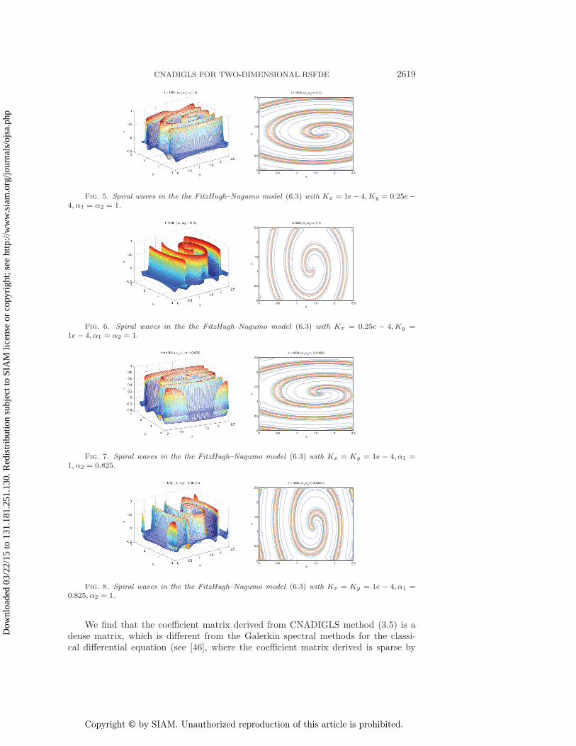
For anisotropic diffusion ratiosKx = 1e−4,Ky

Kx= 0.25 < 1 and Ky = 1e−4, Kx

Ky=

0.25 < 1, wave propagation at t = 1000 is shown in Figures 5 and 6. It is found thatthe spiral wave proceeds to follow an elliptical pattern. For anisotropic fractionalratios α1 = 1, α2

α1= 0.825 < 1 and α2 = 1, α1

α2= 0.825 < 1 with Kx = Ky = 1e − 4,

a contrasting effect on the curvature of the solutions is shown in Figures 7 and 8,reflecting a distinct superdiffusion scale in each of spatial dimensions of the system.These results were first reported in [3].

7. Conclusions. In this paper, a new Crank–Nicolson alternating direction im-plicit Galerkin–Legendre spectral method to solve two-dimensional Riesz space frac-tional nonlinear reaction-diffusion equations was described and demonstrated. We dis-cussed the stability and convergence of the method, which shows that the CNADIGLSmethod is stable and convergent of order 2 in time, and the optimal error estimatein space is also derived by introducing a new orthogonal projector. The CNADIGLSmethod is also extended to solve the fractional FitzHugh–Nagumo model. We presentnumerical experiments to verify the theoretical analysis, which is in good agreementwith the theoretical analysis. These methods and supporting theoretical results can

Dow

nloa

ded

03/2

2/15

to 1

31.1

81.2

51.1

30. R

edis

trib

utio

n su

bjec

t to

SIA

M li

cens

e or

cop

yrig

ht; s

ee h

ttp://

ww

w.s

iam

.org

/jour

nals

/ojs

a.ph

p



x

y

t = 1000, (α1,α

2) = (1,1)

0 0.5 1 1.5 2 2.50

0.5

1

1.5

2

2.5

Fig. 1. Spiral waves in the the FitzHugh–Nagumo model (6.3) with Kx = Ky = 1e − 4, α1 =α2 = 1.

x

y

t = 1000, (α1,α

2) = (1,1)

0 0.5 1 1.5 2 2.50

0.5

1

1.5

2

2.5

Fig. 2. Spiral waves in the the FitzHugh–Nagumo model (6.3) with Kx = Ky = 1e − 5, α1 =α2 = 1.

x

y

t = 1000, (α1,α

2) = (0.75,0.75)

0 0.5 1 1.5 2 2.50

0.5

1

1.5

2

2.5

Fig. 3. Spiral waves in the the FitzHugh–Nagumo model (6.3) with Kx = Ky = 1e − 4, α1 =α2 = 0.75.

x

y

t = 1000, (α1,α

2) = (0.85,0.85)

0 0.5 1 1.5 2 2.50

0.5

1

1.5

2

2.5

Fig. 4. Spiral waves in the the FitzHugh–Nagumo model (6.3) with Kx = Ky = 1e − 4, α1 =α2 = 0.85.

be applied to solve other fractional nonlinear partial differential equations and higher-dimensional problems.

Dow

nloa

ded

03/2

2/15

to 1

31.1

81.2

51.1

30. R

edis

trib

utio

n su

bjec

t to

SIA

M li

cens

e or

cop

yrig

ht; s

ee h

ttp://

ww

w.s

iam

.org

/jour

nals

/ojs

a.ph

p



x

y

t = 1000, (α1,α

2) = (1,1)

0 0.5 1 1.5 2 2.50

0.5

1

1.5

2

2.5

Fig. 5. Spiral waves in the the FitzHugh–Nagumo model (6.3) with Kx = 1e− 4, Ky = 0.25e−4, α1 = α2 = 1.

x

y

t=1000, (α1,α

2) = (1,1)

0 0.5 1 1.5 2 2.50

0.5

1

1.5

2

2.5

Fig. 6. Spiral waves in the the FitzHugh–Nagumo model (6.3) with Kx = 0.25e − 4,Ky =1e− 4, α1 = α2 = 1.

x

y

t = 1000, (α1,α

2) = (1,0.825)

0 0.5 1 1.5 2 2.50

0.5

1

1.5

2

2.5

Fig. 7. Spiral waves in the the FitzHugh–Nagumo model (6.3) with Kx = Ky = 1e − 4, α1 =1, α2 = 0.825.

x

y

t = 1000, (α1,α

2) = (0.825,1)

0 0.5 1 1.5 2 2.50

0.5

1

1.5

2

2.5

Fig. 8. Spiral waves in the the FitzHugh–Nagumo model (6.3) with Kx = Ky = 1e − 4, α1 =0.825, α2 = 1.

We find that the coefficient matrix derived from CNADIGLS method (3.5) is adense matrix, which is different from the Galerkin spectral methods for the classi-cal differential equation (see [46], where the coefficient matrix derived is sparse by

Dow

nloa

ded

03/2

2/15

to 1

31.1

81.2

51.1

30. R

edis

trib

utio

n su

bjec

t to

SIA

M li

cens

e or

cop

yrig

ht; s

ee h

ttp://

ww

w.s

iam

.org

/jour

nals

/ojs

a.ph

p



choosing suitable base functions). Some fast solution techniques were developed in[43, 44, 45, 40, 41] to solve the space fractional differential equations, in which thefractional derivative operators are discretized by the finite difference methods thatyield a coefficient matrix with special structures. For the present method, the ma-trices (see Sx and Sy below (3.9)) derived from the scheme (3.5) do not have specialstructures as do those in [43, 44, 45, 40, 41]. Fast solution techniques for Galerkinspectral methods of the fractional differential equations are still under investigation.Recently, Wang and Yang [42] pointed out that fast solution techniques developed in[43, 44, 45, 40, 41] cannot be applied to the nonconventional Petrov–Galerkin finiteelement method. Fortunately, the present method can be implemented in parallel;therefore, the computational cost can be reduced.

The present method can be extended to solve the three-dimensional problem;all the theoretical results still hold true. However, the Galerkin spectral methodin the present paper cannot be extended to the fractional diffusion equations withvariable diffusivity coefficients, since the Galerkin weak formulation loses coercivity;see Lemma 3.2 in [42]. Maybe the Petrov–Galerkin spectral method can be developedto solve the fractional diffusion equations with variable coefficients (see [42], where thePetrov–Galerkin finite element method was proved to be well posed). If we drop the

term τ2

4 (LxLy(un+1−un), v) in (3.5), we obtain the non-ADI method; the theoretical

results still hold true for such a case. They also hold true for one-dimensional andthree-dimensional fractional diffusion equations.

Acknowledgments. The first author thanks the School of Mathematical Sci-ences at QUT for supporting this research. The authors wish to thank the refereesfor their constructive comments and suggestions which improved the present paper.

REFERENCES

[1] V. V. Anh and N. N. Leonenko, Spectral analysis of fractional kinetic equations with randomdata, J. Statist. Phys., 104 (2001), pp. 1349–1387.

[2] C. Bernardi and Y. Maday, Spectral methods, Handb. Numer. Anal. Vol. V, North-Holland,Amsterdam, 1997, pp. 209–485.

[3] A. Bueno-Orovio, D. Kay, and K. Burrage, Fourier spectral methods for fractional-in-space reaction-diffusion equations, BIT, to appear 2014. Available online athttp://eprints.maths.ox.ac.uk/1551/.

[4] C. Canuto, M. Y. Hussaini, A. Quarteroni, and T. A. Zang, Spectral Methods, Fundamen-tals in Single domains, Springer-Verlag, Berlin, 2006.

[5] W. H. Deng, Finite element method for the space and time fractional Fokker–Planck equation,SIAM J. Numer. Anal., 47 (2008), pp. 204–226.

[6] V. J. Ervin, N. Heuer, and J. P. Roop, Numerical approximation of a time dependent,nonlinear, space-fractional diffusion equation, SIAM J. Numer. Anal., 45 (2007) , pp. 572–591.

[7] V. J. Ervin and J. P. Roop, Variational solution of fractional advection dispersion equationson bounded domains in Rd, Numer. Methods Partial Differential Equations, 23 (2007), pp.256–281.

[8] J. F. Huang, N. N. Nie, and Y. F. Tang, A second order finite difference-spectral methodfor space fractional diffusion equation, SCIENCE CHINA Mathematics, 136 (2013), pp.521–537.

[9] A. A. Kilbas, H. M. Srivastava, and J. J. Trujillo, Theory and Applications of FractionalDifferential Equations, Elsevier, Netherlands, 2006.

[10] N. N. Leonenko, M. M. Meerschaert, and A. Sikorskii, Fractional Pearson diffusions, J.Math. Anal. Appl., 403 (2013), pp. 532–546.

[11] J. C. Li, Y. Q. Huang, and Y. P. Lin, Developing finite element methods for Maxwell’sequations in a Cole–Cole dispersive medium, SIAM J. Sci. Comput., 33 (2011), pp. 3153–3174.

Dow

nloa

ded

03/2

2/15

to 1

31.1

81.2

51.1

30. R

edis

trib

utio

n su

bjec

t to

SIA

M li

cens

e or

cop

yrig

ht; s

ee h

ttp://

ww

w.s

iam

.org

/jour

nals

/ojs

a.ph

p

http://eprints.maths.ox.ac.uk/1551/



[12] C. P. Li and F. H. Zeng, Finite difference methods for fractional differential equations, In-ternat. J. Bifur. Chaos Appl. Sci. Engrg., 22 (2012), 1230014.

[13] C. P. Li, F. H. Zeng, and F. Liu, Spectral approximations to the fractional integral andderivative, Fract. Calc. Appl. Anal., 15 (2012), pp. 383–406.

[14] C. P. Li, Z. G. Zhao, and Y. Q. Chen, Numerical approximation of nonlinear fractional dif-ferential equations with subdiffusion and superdiffusion, Comput. Math. Appl., 62 (2011),pp. 855–875.

[15] X. J. Li and C. J. Xu, A space-time spectral method for the time fractional diffusion equation,SIAM J. Numer. Anal., 47 (2009), pp. 2108–2131.

[16] Y. M. Lin and C. J. Xu, Finite difference/spectral approximations for the time-fractionaldiffusion equation, J. Comput. Phys., 225 (2007), pp. 1533–1552.

[17] R. Lin, F. Liu, V. Anh, and I. Turner, Stability and convergence of a new explicit finite-difference approximation for the variable-order nonlinear fractional diffusion equation,Appl. Math. Comput., 212 (2009), pp. 435–445.

[18] F. Liu, V. Anh, and I. Turner, Numerical solution of the space fractional Fokker–Planckequation, J. Comput. Appl. Math., 166 (2004), pp. 209–219.

[19] F. Liu, S. Chen, I. Turner, K. Burrage, and V. Anh Numerical simulation for two-dimensional Riesz space fractional diffusion equations with a nonlinear reaction term,Cent. Eur. J. Phys., 11 (2013), pp. 1221–1232.

[20] F. Liu, P. Zhuang, V. Anh, I. Turner, and K. Burrage, Stability and convergence ofthe difference methods for the space-time fractional advection-diffusion equation, J. Appl.Math. Comput., 91 (2007), pp. 12–20.

[21] F. Liu, C. Yang, and K. Burrage, Numerical method and analytical technique of the modifiedanomalous subdiffusion equation with a nonlinear source term, J. Comput. Appl. Math.,231 (2009), pp. 160–176.

[22] H. P. Ma and W. W. Sun, Optimal error estimates of the Legendre–Petrov–Galerkin methodfor the Korteweg-de Vries equation, SIAM J. Numer. Anal., 39 (2001), pp. 1380–1394.

[23] R. Metzler and J. Klafter, The random walk’s guide to anomalous diffusion: A fractionaldynamics approach, Phys. Rep., 339 (2000), pp. 1–77.

[24] R. Magin, O. Abdullah, D. Baleanu, and X. Zhou, Anomalous diffusion expressed throughfractional order differential operators in the Bloch-Torrey equation, J. Magn. Reson., 190(2008), pp. 255–270.

[25] M. M. Meerschaert and A. Sikorskii, Stochastic Models for Fractional Calculus, De GruyterStud. Math. 43, Walter de Gruyter, Berlin, 2012.

[26] M. M. Meerschaert and C. Tadjeran, Finite difference approximations for fractionaladvection-dispersion, J. Comput. Appl. Math., 172 (2004), pp. 65–77.

[27] M. M. Meerschaert, J. Mortensenb, and S. W. Wheatcraft, Fractional vector calculusfor fractional advection-dispersion, Phys. A, 367 (2006), pp. 181–190.

[28] K. Mustapha and W. McLean, Piecewise-linear, discontinuous Galerkin method for a frac-tional diffusion equation, Numer. Algorithms, 56 (2011), pp. 159–184.

[29] K. Mustapha and W. McLean, Uniform convergence for a discontinuous Galerkin, timestepping method applied to a fractional diffusion equation, IMA J. Numer. Anal., 32 (2012),pp. 906–925.

[30] K. Mustapha and W. McLean, Superconvergence of a discontinuous Galerkin method forfractional diffusion and wave equations, SIAM J. Numer. Anal., 51 (2013), pp. 491–515.

[31] E. D. Nezza, G. Palatucci, and E. Valdinoci, Hitchhiker’s guide to the fractional Sobolevspaces, Bull. Sci. Math., 136 (2012), pp. 521–573.

[32] J. A. Ochoa-Tapia, F. J. Valdes-Parada, and J. Alvarez-Ramirez, A fractional-orderDarcy’s law, Phys. A, 374 (2007), pp. 1–14.

[33] I. Podlubny, Fractional Differential Equations, Acdemic Press, San Diego, 1999.[34] A. Quarteroni and A. Valli, Numerical Approximation of Partial Differential Equations,

Springer Ser. Comput. Math., 23, Springer-Verlag, Berlin, 1994.[35] J. P. Roop, Variational Solution of the Fractional Advection Dispersion Equation, Ph.D.

thesis, Clemson University, Clemson, SC, 2004.[36] S. G. Samko, A. A. Kilbas, and O. I. Marichev, Fractional Integrals and Derivatives: Theory

and Applications, Gordon and Breach Science Publishers, Yverdon-les-Bains, Switzerland,1993.

[37] J. Shen, T. Tang, and L. L. Wang, Spectral Methods: Algorithms, Analysis and Applications,Springer Ser. Comput. Math. 41, Springer, Heidelberg, 2011.

[38] J. Shen, Efficient spectral-Galerkin method I. Direct solvers for second- and fourth-order equa-tions using Legendre polynomials, SIAM J. Sci. Comput., 15 (1994), pp. 1489–1505.

[39] F. J. Valdes-Parada, J. A. Ochoa-Tapia, and J. Alvarez-Ramirez, Effective medium equa-

Dow

nloa

ded

03/2

2/15

to 1

31.1

81.2

51.1

30. R

edis

trib

utio

n su

bjec

t to

SIA

M li

cens

e or

cop

yrig

ht; s

ee h

ttp://

ww

w.s

iam

.org

/jour

nals

/ojs

a.ph

p



tions for fractional Fick’s law in porous media, Phys. A, 373 (2007), pp. 339–353.[40] H. Wang and N. Du, A fast finite difference method for three-dimensional time-dependent

space-fractional diffusion equations and its efficient implementation, J. Comput. Phys.,253 (2013), pp. 50–63.

[41] H. Wang and N. Du, Fast alternating-direction finite difference methods for three-dimensionalspace-fractional diffusion equations, J. Comput. Phys., 258 (2014), pp. 305–318.

[42] H. Wang. and D. P. Yang Wellposedness of variable-coefficient conservative fractional ellipticdifferential equations, SIAM J. Numer. Anal., 51 (2013), pp. 1088–1107.

[43] H. Wang, K. X. Wang, and T. Sircar, A direct O(N log2 N) finite difference method forfractional diffusion equations, J. Comput. Phys., 229 (2010), pp. 8095–8104.

[44] H. Wang and K. X. Wang, An O(N log2 N) alternating-direction finite difference method fortwo-dimensional fractional diffusion equations, J. Comput. Phys., 230 (2011), pp. 7830–7839.

[45] H. Wang and T. S. Basu, A fast finite difference method for two-dimensional space-fractionaldiffusion equations, SIAM J. Sci. Comput., 34 (2012), pp. A2444–A2458.

[46] H. Wu, H. P. Ma, and H. Y. Li, Optimal error estimates of the Chebyshev–Legendre spectralmethod for solving the generalized Burgers equation, SIAM J. Numer. Anal., 41 (2003),pp. 659–672.

[47] F. Zeng, C. Li, F. Liu, and I. Turner The use of finite difference/element approaches forsolving the time-fractional subdiffusion equation, SIAM J. Sci. Comput., 35 (2013), pp.A2976–A3000.

[48] P. Zhuang, F. Liu, V. Anh, and I. Turner, Numerical methods for the variable-order frac-tional advection-diffusion equation with a nonlinear source term, SIAM J. Numer. Anal.,47 (2009), pp. 1760–1781.

Dow

nloa

ded

03/2

2/15

to 1

31.1

81.2

51.1

30. R

edis

trib

utio

n su

bjec

t to

SIA

M li

cens

e or

cop

yrig

ht; s

ee h

ttp://

ww

w.s

iam

.org

/jour

nals

/ojs

a.ph

p

a crank--nicolson adi spectral method for a two ...eprints.qut.edu.au/82655/8/82655_pubver.pdf ·...

Documents