ON THE UNCERTAINTY MODELING AND VALIDATIONFOR EXTERNAL STORES AERODYNAMICS

Sebastian Heinze1, Ulf Ringertz2 and Dan Borglund3

Department of Aeronautical and Vehicle EngineeringRoyal Institute of Technology (KTH)

Teknikringen 8, SE - 100 44, Stockholm, Swedene-mail: 1sepp@kth.se, 2rzu@kth.se and 3dodde@kth.se

Key words: Aeroelasticity, aerodynamic uncertainty, modeling and validation, robustflutter analysis, wind tunnel experiments

Abstract. A wind tunnel model representing a generic delta wing configuration withexternal stores is considered for flutter investigations. Complex eigenvalues are esti-mated for the wind tunnel model for airspeeds up to the flutter limit, and compared toeigenvalues predicted by a numerical model. The impact of external stores mountedto the wing tip is investigated both experimentally and numerically, and besides theimpact of the stores as such, the capability of the numerical model to account for in-creasing model complexity is investigated. An uncertainty approach based on robustflutter analysis is demonstrated to account for modeling imperfections. Uncertaintymodeling issues and the reliability of uncertainty models are discussed. Provided thatthe present uncertainty mechanism can be determined, it is found that available uncer-tainty tools may be used to efficiently compute robust flutter boundaries.

1 INTRODUCTION

Flutter testing is rarely performed on full scale aircraft due to the high risk for struc-tural damage and failure. Instead, flutter boundaries are computed based on a nu-merical model of the aircraft, and flight testing under less critical conditions can beperformed to collect data for validation of the numerical model. Clearly, problemsarise when the flight test data shows deviation from the numerically predicted data.Deviations are likely to occur for any aircraft configuration, since model imperfectionsand simplifications always lead to some uncertainty in the numerical model, and thequestion arises what impact these uncertainties have on the predicted flutter bound-aries.

In most cases, some parts of the numerical model, such as the mass properties of dif-ferent components, are well known, whereas other elements, like the aerodynamicloads in some region of a wing with complex geometry, are known to be subject touncertainty. Earlier studies1,2,3,4 have shown how aerodynamic uncertainties can beintroduced in the numerical model based on physical reasoning and known modelingdifficulties. This study aims at demonstrating how uncertainties can be introduced

1

in the numerical model, and how data points collected at subcritical conditions maybe used to establish an uncertainty model that is capable of producing reliable flutterboundaries.

In the present study, a wind tunnel model was designed to demonstrate and evaluateuncertainty modeling approaches. A fairly simple wing geometry and structure arechosen to minimize the errors introduced by modeling simplifications. The modelcomplexity is then increased gradually, and analyses and experiments are performedfor each configuration to detect modeling difficulties. An external store in the form ofa wing tip missile is used for this purpose, and the impact on the flutter behavior isinvestigated, as well as the capability of flutter analysis tools to provide correct resultsfor increasing model complexity. In cases where the numerical predictions deviatefrom the experimental results, robust analysis is applied and uncertainty modelingapproaches are evaluated.

2 EXPERIMENTAL SETUP

The considered model is a generic delta wing configuration as shown in Figure 1 witha semi-span of 0.88 m. The wing is mounted vertically on the floor in the low-speed

Figure 1: Delta wing mounted in the low-speed wind tunnel L2000 at KTH.

wind tunnel L2000 at the Royal Institute of Technology (KTH). Due to the high riskinvolved in flutter testing, it was found convenient to design a low-cost wind tunnel

2

model with a low level of complexity. The wing consists of a glass fiber plate withcarbon fiber stiffeners to obtain the desired structural properties. The wing can easilybe equipped with external stores, such as an underwing missile and a wing tip missile.In the present study, the impact of a wing tip store will be investigated.

2.1 STRUCTURAL DESIGN

The wind tunnel model is meant to represent a generic delta wing configuration of afighter aircraft. Due to the length and velocity scales imposed by the wind tunnel envi-ronment, some properties such as the Mach number of the model will not represent thefull scale model. The model was however scaled in terms of the structural propertieswith respect to the aeroelastic behavior. The objective was to obtain eigenfrequenciesf such that the reduced frequencies k = 2πf ·L/V are the same for both model and fullscale aircraft, where L is a reference length, and the velocity V is chosen at a typicalflight condition.

In the present case, it was found that both the length scaling and the velocity scalingfactors between model and full-scale aircraft are in the order of 10, making the fre-quency scaling factor equal to one. Therefore, structural eigenfrequencies of the modelwere chosen to be equal to the eigenfrequencies of a representative full-scale structure.Since flutter behavior typically is governed by the lower eigenfrequencies of a struc-ture, the first bending and the first torsional eigenfrequencies were emphasized.

To obtain specific eigenfrequencies as determined by the aeroelastic scaling, a few de-sign parameters were defined in the structural design. In general, both eigenfrequen-cies and eigenmode shapes can be controlled by the mass and stiffness distribution.In the present study, a fixed wing geometry was assumed, and a glass fiber compos-ite plate was considered as a baseline structure. Carbon fiber composite spars wereattached to the composite plate to control the structural properties of the wing. Twospars were mounted on both the upper and lower side of the wing, and the spar di-mensions and positions were chosen to obtain the desired eigenfrequencies. The modeshapes were not designed specifically.

2.2 EXTERNAL STORE

The main focus of the study is to investigate the aerodynamic impact of an externalstore on the flutter behavior. A realistic wing tip missile was therefore manufacturedand mounted to the wing tip as shown in Figure 2. The missile is mounted to a launcherbeam that is assumed to be rigidly connected to the wing tip. Different configurationswere considered to identify the aerodynamic impact of different missile componentson the flutter behavior of the wing. Figure 3 shows the five considered configurations.In order to reduce the effects on the flutter speed due to structural differences betweenthe different configurations, mass balancing was used to compensate for different com-ponents once removed from the wind tunnel model. The mass balancing for the finswas located within the missile body, whereas the mass balancing for the missile was

3

Figure 2: Wing tip external store.

located within the launcher beam to maintain the aerodynamic shape of the wing tipregion.

3 NUMERICAL MODEL

Numerical models of the delta wing were generated in both Nastran5 and ZAERO6.The model is composed of shell elements for the wing, mass elements for the missile,and aerodynamic panels for both wing and missile. The missile assembly was assumedto be rigid.

3.1 STRUCTURAL MODELING

The geometry of the structural elements of the wing plate was defined such that thelocation of the carbon fiber spars coincides with the location of structural grid pointsin order to allow for accurate modeling of the different material properties. NastranCQUADR elements were selected for connecting the structural grid points of the wingplate. Figure 4 shows the discretization of the structural elements of the wing plate.Note that the location of the carbon fiber stiffeners is indicated in the Figure. Theirregular discretization in the wing tip region is chosen to allow for accurate modelingof the launcher beam attachment.

Material properties were derived in several steps, starting by the glass fiber plate with-

4

Config. 3:Rear fins only

Config. 4:No fins

Config 5:No missileCanard fins only

Config. 2:

Configuration 1: Full missile

Figure 3: Uncertain patches in wing tip region.

Structural elements Aerodynamic panels

Figure 4: Discretization of the numerical model.

out the carbon fiber spars. Vibration testing of the plate was performed to obtain mate-rial data by matching the measured eigenfrequencies to the eigenfrequencies predictedby the numerical model. The wing was freely supported to exclude effects due to im-perfections of the boundary conditions once mounted to the wind tunnel floor.

Material data from the manufacturer were used to determine material properties ofthe carbon fiber spars. Once attached to the glass fiber wing, another vibration testwas performed to validate the material data. After that, the wing was mounted into

5

the wind tunnel, and yet another vibration test was performed. The measured eigen-frequencies appeared to be somewhat lower than expected for a rigidly clamped wing,and it was found that introducing some flexibility in the numerical model of the clamp-ing improved the frequency matching. The flexibility was chosen such that the firstand second eigenfrequencies predicted by the numerical model were within 0.1 Hzfrom the measured eigenfrequencies from the vibration testing.

The missile was assumed to be rigid, and only the mass properties of the missile weremodeled. A grid point representing the degrees of freedom of the missile assembly wasdefined and attached to the wing tip. In the experimental setup, the missile launcher isrigidly connected to the wing tip along the entire tip chord, thus eliminating chordwisebending deformations of the wing tip region. Masses for the various components ofthe missile were then rigidly attached to that grid point.

The structural damping was neglected in the structural model, and it was assumedthat this simplification results in slightly conservative flutter predictions without anysignificant impact on the general flutter behavior. The numerical approaches presentedin the following sections are based on a model without structural damping, but couldeasily be modified to include damping.

3.2 AERODYNAMIC PANELS

The aerodynamic modeling was performed in both Nastran and ZAERO. NastranCAERO1 elements were used to model aerodynamic panels for computation of doublet-lattice7 aerodynamic loads. The wing surface was covered by 12 spanwise times 14chordwise lifting surfaces equally distributed on the wing area. The launcher beamand missile body were modeled as flat panels parallel to the wing surface, since it wasassumed that in-plane airloads generated by panels perpendicular to the wing sur-face can be neglected in the flutter analysis. Depending on the configuration, between200 (Config. 5) and 402 (Config. 1) aerodynamic panels were defined. In Figure 4, theNastran aerodynamic panels for the full missile configuration are shown.

The ZAERO aerodynamic model using CAERO7 elements utilizes the same discretiza-tion as the Nastran model for the wing, the missile launcher beam, and the missile fins.The missile body, however, was modeled using BODY7 elements.

To connect the structure and the aerodynamic panels, a surface spline was defined forthe wing plate using a SPLINE1 in both Nastran and ZAERO, and a beam spline wasdefined for connecting the missile panels to the grid point defining the missile motion,using SPLINE5 in Nastran and ATTACH in ZAERO.

4 FLUTTER RESULTS

In most applications, flutter testing of real aircraft is restricted to subcritical airspeedsdue to the high risk involved in operating the aircraft in flutter conditions. As the air-speed approaches the flutter stability limit, the aeroelastic damping of the structure

6

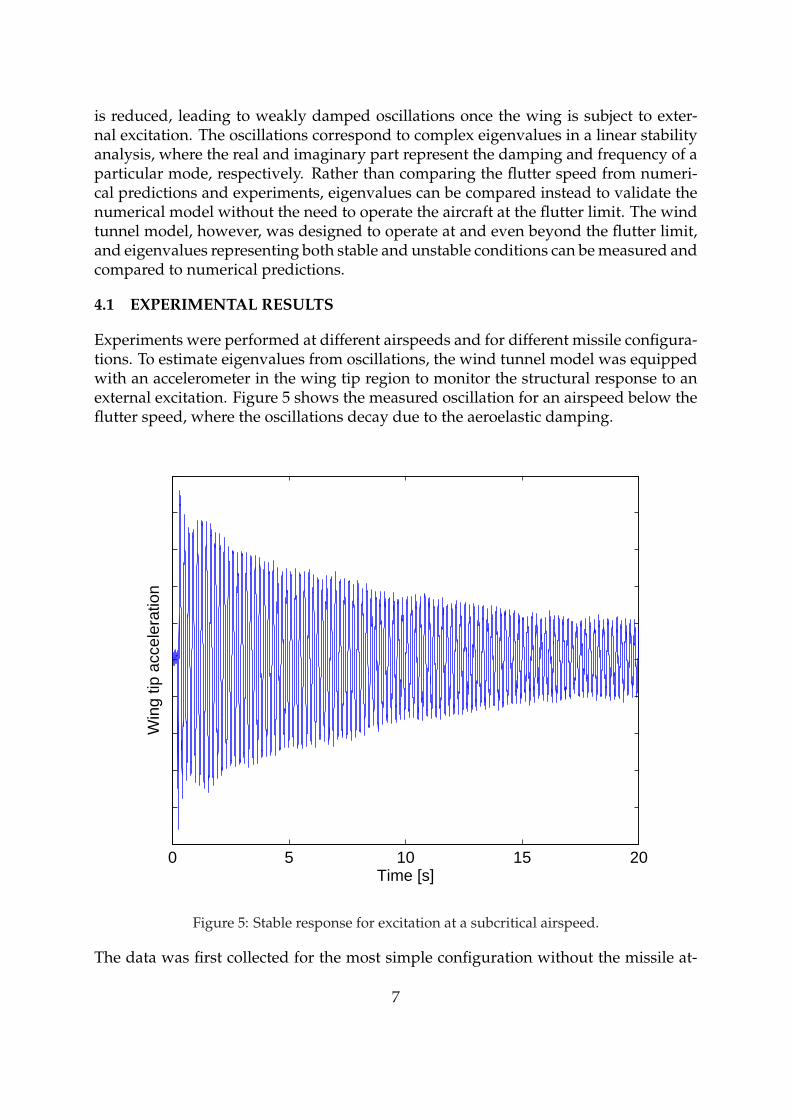
is reduced, leading to weakly damped oscillations once the wing is subject to exter-nal excitation. The oscillations correspond to complex eigenvalues in a linear stabilityanalysis, where the real and imaginary part represent the damping and frequency of aparticular mode, respectively. Rather than comparing the flutter speed from numeri-cal predictions and experiments, eigenvalues can be compared instead to validate thenumerical model without the need to operate the aircraft at the flutter limit. The windtunnel model, however, was designed to operate at and even beyond the flutter limit,and eigenvalues representing both stable and unstable conditions can be measured andcompared to numerical predictions.

4.1 EXPERIMENTAL RESULTS

Experiments were performed at different airspeeds and for different missile configura-tions. To estimate eigenvalues from oscillations, the wind tunnel model was equippedwith an accelerometer in the wing tip region to monitor the structural response to anexternal excitation. Figure 5 shows the measured oscillation for an airspeed below theflutter speed, where the oscillations decay due to the aeroelastic damping.

0 5 10 15 20Time [s]

Win

g tip

acc

eler

atio

n

Figure 5: Stable response for excitation at a subcritical airspeed.

The data was first collected for the most simple configuration without the missile at-

7

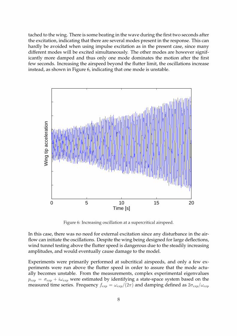
tached to the wing. There is some beating in the wave during the first two seconds afterthe excitation, indicating that there are several modes present in the response. This canhardly be avoided when using impulse excitation as in the present case, since manydifferent modes will be excited simultaneously. The other modes are however signif-icantly more damped and thus only one mode dominates the motion after the firstfew seconds. Increasing the airspeed beyond the flutter limit, the oscillations increaseinstead, as shown in Figure 6, indicating that one mode is unstable.

0 5 10 15 20Time [s]

Win

g tip

acc

eler

atio

n

Figure 6: Increasing oscillation at a supercritical airspeed.

In this case, there was no need for external excitation since any disturbance in the air-flow can initiate the oscillations. Despite the wing being designed for large deflections,wind tunnel testing above the flutter speed is dangerous due to the steadily increasingamplitudes, and would eventually cause damage to the model.

Experiments were primarily performed at subcritical airspeeds, and only a few ex-periments were run above the flutter speed in order to assure that the mode actu-ally becomes unstable. From the measurements, complex experimental eigenvaluespexp = σexp + iωexp were estimated by identifying a state-space system based on themeasured time series. Frequency fexp = ωexp/(2π) and damping defined as 2σexp/ωexp

8

are then extracted from the eigenvalues. Figure 7 shows the resulting damping andfrequency versus airspeed. The flutter speed lies between 25 and 26 m/s, where thedamping crosses zero, corresponding to a purely imaginary eigenvalue. Similar exper-iments were performed for all configurations. Note that numerical predictions, thatwere obtained as described in the next Section, are included in the Figure.

4.2 NOMINAL FLUTTER ANALYSIS

The nominal analysis is performed by solving the flutter equation

F 0(p,M)η =

[M 0p

2 +

(L

V

)2

K0 − ρL2

2Q0(p,M)

]η = 0 (1)

where M 0, K0, and Q0(p,M) are the nominal mass, stiffness, and aerodynamic ma-trices that define the nominal flutter matrix F 0. The airspeed, air density and Machnumber are denoted V , ρ, and M , respectively, and L is the reference length used tomake the equation nondimensional. The flutter equation is a nonlinear eigenvalueproblem with complex eigenvalues p = g + ik and vectors of modal coordinates η.The flutter stability limit is found as the real part of the eigenvalue becomes zero. Theimaginary part of the eigenvalue is the reduced frequency k = ω · L/V , and the realpart g = σ · L/V is a measure of the damping of the system. As for the eigenvaluesestimated by the experimental time series, the damping is then defined as 2g/k. Notethat ω and σ used in the analysis correspond to ωexp and σexp from the experiment,respectively.

In Figure 7, the numerical results are shown along with the measurements. The com-parison shows that the flutter speed is predicted accurately by the numerical model.Note that the experimental data is more noisy for lower velocities. This is due to thehigher aeroelastic damping, making the oscillations decay faster, which leads to shortersampling times and therefore less accurate values for frequency and damping. In gen-eral, however, the analysis predicts both frequency and damping very well.

There is also a slight offset in the frequency, which may be due to an inaccurate struc-tural model. It was for example found that the frequency drops by 0.1 Hz if the tem-perature in the tunnel increases by 3 degrees Celsius. Therefore, it is expected thatthe measured frequencies are slightly lower as the closed-loop wind tunnel is underoperation and increases the air temperature.

4.3 INFLUENCE OF EXTERNAL STORES

When attaching the missile to the wing, the flutter behavior is expected to change bothin the analysis and in the experiment. Since mass balancing was used to account for themissile components, however, all configurations should have similar structural prop-erties, and the main differences are expected to be due to different aerodynamic loads.The missile was attached to the wing in several steps, beginning with the missile body

9

18 20 22 24 26 28 30

4.8

5

5.2

5.4

5.6F

requ

ency

[Hz]

18 20 22 24 26 28 30−0.03

−0.02

−0.01

0

0.01

0.02

Velocity [m/s]

Dam

ping

NastranZAEROExperiment

Figure 7: Comparison of numerical and experimental results for the configuration without themissile.

(Config. 4). Flutter results from this configuration are shown in Figure 8. The Fig-ure shows that the quality of the damping data is somewhat lower than in the casebefore. Nevertheless, the damping obtained in the experiments agrees with the pre-diction fairly well. Again, there is a constant offset in the frequency, but the frequencytrend is captured well. Nastran and ZAERO produce very similar results for this con-figuration.

In the next step, the canard fins were attached to the model. The frequency and damp-ing curves for this configuration are shown in Figure 9. Compared to the case withoutcanard fins, the flutter speed was reduced by 1.5 m/s in the analysis. There is somescatter in the measured damping, but it seems that the mean value fits reasonably wellto the numerical results. The predicted frequency follows the measured values nicely,although the slope of the predicted curve is slightly less than in the experiments.

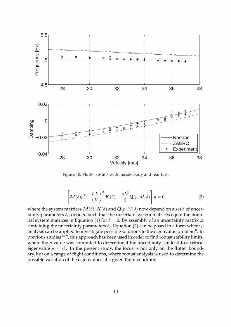
Next, the canard fins were removed again and the rear fins attached to the missile. Re-sults from these investigations are shown in Figure 10. The rear fins increase the flutterspeed significantly, which is predicted both in the analysis and found in the experimen-

10

22 24 26 28 30 32 344.5

5

5.5F

requ

ency

[Hz]

22 24 26 28 30 32 34−0.03

−0.02

−0.01

0

0.01

0.02

Velocity [m/s]

Dam

ping

NastranZAEROExperiment

Figure 8: Flutter results with missile body attached.

tal investigations. The Nastran and ZAERO damping predictions deviate slightly fromeach other, with the experimental values being located between these curves. Nastranis slightly conservative, whereas ZAERO overpredicts the flutter speed. The frequencytrend is predicted well, but again there is an offset between analysis and experiment.

Finally, the complete configuration was considered by attaching the canard wings, withresults as shown in Figure 11. As before, the canard wings lead to a destabilization ofthe wing. In the analysis, this can be seen by a reduction of the predicted flutter speedfrom 34 to 32 m/s for the Nastran model and from 36 to 34 m/s for ZAERO. The ex-periment is again in between the predictions by Nastran and ZAERO, with Nastranbeing slightly conservative. There is also a more pronounced scatter in the experimen-tal damping data. The frequency is again predicted well with a slight constant offset.

The investigations of the different configurations show that the numerical model isfairly accurate. As the rear fins are included, the predictions by Nastran and ZAEROdeviate from each other, with the experimental data lying in between these predic-tions. In the following Section, a robust approach will be presented where uncertainty

11

20 22 24 26 28 304.6

4.8

5

5.2

5.4

Fre

quen

cy [H

z]

20 22 24 26 28 30−0.03

−0.02

−0.01

0

0.01

0.02

Velocity [m/s]

Dam

ping

NastranZAEROExperiment

Figure 9: Flutter results with missile body and canard fins.

modeling will be used to account for modeling imperfections in order to derive robustflutter bounds that capture the experimental data entirely. Due to the similar behaviorof the Nastran and the ZAERO models, the robust approach is based on the Nastranmodel only. It is assumed that a robust approach based on the ZAERO model wouldproduce similar results.

5 ROBUST APPROACH

Comparison between the experimental and predicted eigenvalues indicates that thenumerical model captures the flutter behavior fairly well. As the missile is attached tothe wing, however, the analysis is not as accurate, in particular as the rear fins are in-cluded. It is therefore assumed that the error is due to modeling imperfections that canbe accounted for by introducing uncertainties in the numerical model. Instead of com-puting nominal eigenvalues from Equation (1), the objective is to compute eigenvaluebounds by considering an uncertain flutter equation according to

12

28 30 32 34 36 384.5

5

5.5F

requ

ency

[Hz]

28 30 32 34 36 38−0.04

−0.02

0

0.02

Velocity [m/s]

Dam

ping

NastranZAEROExperiment

Figure 10: Flutter results with missile body and rear fins.

[M (δ)p2 +

(L

V

)2

K(δ)− ρL2

2Q(p,M, δ)

]η = 0 (2)

where the system matrices M(δ), K(δ) and Q(p,M, δ) now depend on a set δ of uncer-tainty parameters δi, defined such that the uncertain system matrices equal the nomi-nal system matrices in Equation (1) for δ = 0. By assembly of an uncertainty matrix ∆containing the uncertainty parameters δi, Equation (2) can be posed in a form where µanalysis can be applied to investigate possible solutions to the eigenvalue problem8. Inprevious studies1,2,9, this approach has been used in order to find robust stability limits,where the µ value was computed to determine if the uncertainty can lead to a criticaleigenvalue p = ik. In the present study, the focus is not only on the flutter bound-ary, but on a range of flight conditions, where robust analysis is used to determine thepossible variation of the eigenvalues at a given flight condition.

13

24 26 28 30 32 34 364.5

5

5.5F

requ

ency

[Hz]

24 26 28 30 32 34 36−0.04

−0.02

0

0.02

Velocity [m/s]

Dam

ping

NastranZAEROExperiment

Figure 11: Flutter results with complete missile.

5.1 UNCERTAINTY MODELING

Uncertainty modeling based on uncertain system matrices as discussed above is conve-nient for introducing uncertainties based on physical reasoning. In many cases, someparts of the nominal model are known to contain uncertainty due to modeling difficul-ties, whereas other parts may be known to be accurately modeled. In the present case,the structural model has been tuned to fit experimental data from vibration testingexperiments, and is considered accurate.

Uncertainty is only introduced in the aerodynamic matrix, where a modeling approachas presented in Refs.1,2 is used to allow for uncertainties in selected aerodynamic pan-els only. The aerodynamic matrix Q0 is therefore partitioned into left and right par-titions Q0(k, M) = L · R(k,M), where R(k, M) computes the pressure coefficients ineach aerodynamic panel as a function of the modal coordinates, and L computes modalforces from the pressure coefficients.

Aerodynamic uncertainty is introduced such that the pressure coefficients for a subset

14

of aerodynamic panels i is allowed to vary according to cpi = cpi0(1+wiδi), where cpi0 isthe nominal pressure coefficient, and wi is a real valued uncertainty bound that is cho-sen such that the uncertainty parameters |δi| ≤ 1. As shown in Ref.2, the aerodynamicmatrix can then be written

Q = Q0 + QL∆QR (3)

where ∆ is a block diagonal matrix containing the uncertainty parameters δi, and QL

and QR are scaling matrices based on R, L and wi. Due to the bounds on δi and thestructure of ∆, the uncertainty matrix fulfills ∆ ∈ S∆ with

S∆ = {∆ : ∆ ∈ ∆ and σ̄(∆) ≤ 1} (4)

where ∆ denotes the block structure of the uncertainty matrix, and σ̄(·) denotes themaximum singular value.

5.2 µ-p ANALYSIS

This uncertainty description is then inserted in the uncertain flutter equation (2) andthe flutter equation can be written

{I +

ρL2

2QRF−1

0 QL︸ ︷︷ ︸−F

∆

}QRη︸︷︷︸

w

= 0. (5)

With the uncertain flutter equation in the form (I−F (p)∆)w = 0, so-called µ-analysis10

can be applied to Equation (5). For a given system matrix F (p), the structured singularvalue

µ(p) = µ[F (p)] =1

min∆{σ̄(∆) : ∆ ∈ ∆, det(I − F (p)∆) = 0} (6)

is defined based on the smallest norm σ̄(∆) that makes p an eigenvalue to the uncertainflutter equation for a given flight condition. Note that there are no tools for computingthe µ value exactly for any structured uncertainty ∆. Instead, upper and lower boundsof the µ value can be computed, for example using the µ Toolbox in Matlab11. In orderto obtain a robust flutter boundary, the upper bound of the µ value will be consideredin the following analysis.

Figure 12 shows an example of the variation of the upper-bound µ value in the complexplane for a region around the first two eigenvalues of the nominal flutter equation. TheFigure shows that there are peaks at the locations of the nominal eigenvalues. For fixedvalues of µ, elliptic areas can be identified around these eigenvalues, where the Figureindicates the areas corresponding to µ = 1. From Equation (6) and the bounds on ∆

15

Figure 12: µ value in the complex plane.

stated in Equation (4), the following criteria hold:

µ(p) ≥ 1 ⇔ p is an eigenvalue of (2) for some ∆ ∈ S∆ (7)µ(p) < 1 ⇔ p is not an eigenvalue of (2) for any ∆ ∈ S∆ (8)

As described in Ref8, the criterion (7-8) can be used to compute robust eigenvalueswith minimum or maximum damping, from which damping bounds for a particularmode can be extracted and compared to experimental data. As described in the nextSection, the µ-p formulation also allows for straightforward model validation based onexperimental estimates of flutter eigenvalues.

5.3 UNCERTAINTY VALIDATION

As uncertainty is introduced into the nominal system, not only the structure of theuncertainty, but also the bounds wi have to be specified. Naturally, the bounds havesignificant impact on the robust flutter results. A too small magnitude may lead toresults not capable of capturing the behavior of the system, whereas a too large bound

16

leads to flutter results being too conservative. In the present study, uncertainty valida-tion will be used to estimate the uncertainty bound8. For a given uncertainty structure,the minimum bound that is required to include the experimental results into the rangeof the robust predictions is selected. Note that in this study, only the most criticalmode was considered with the eigenvalue measured at different velocities. Figure 13demonstrates different approaches for the uncertainty validation based on a measuredeigenvalue. The Figure shows the regions that bound the uncertain eigenvalue for

0-0.01-0.02-0.03

p-validation

0.76

0.75

0.74g-validation

k-validation

Computed pMeasured p

Im(p)

Re(p)

Figure 13: Different validation approaches for a representative case.

µ = 1 for different uncertainty norms. In the present study, it was found that the aero-dynamic uncertainty allows for a circular variation of the eigenvalue. Validation basedon eigenvalues (p-validation) results in a bound that assures that measured eigenvalueis a solution to the uncertain flutter Equation (2). According to Equations (7) and (8),the least possible uncertainty bound for a set of measured eigenvalues pexp is foundwhen µ(pexp) ≥ 1 for all considered pexp, and when µ(p̂exp) = 1 for at least one measuredeigenvalue p̂exp, which in this case would be the decisive eigenvalue for the bound.

In the present study, comparison between the measured and nominal eigenvaluesshows that the imaginary part corresponding to the frequency differs more than thereal part corresponding to the damping. Due to the larger magnitude of the frequency,however, the relative error of the frequency is much less than the relative error of thedamping and may possibly be neglected. It was considered inconvenient to performp-validation, that aims on matching both the real and the imaginary part of the eigen-value and therefore leads to unrealistically high uncertainty levels in order to capturethe slight frequency offset observed in the nominal results. Since the damping is morecritical than the frequency in flutter analysis, focus will be on possible deviations inthe real part of the eigenvalues due to the uncertainty. In Figure 13, this approach isdenoted g-validation. Another approach, k-validation, may for example be used forthe validation of structural uncertainties based on data from ground vibration testing,where the structural damping (corresponding to g) may have minor importance, and

17

where uncertainties in the mass- and stiffness distribution have a more significant im-pact on the frequency.

In this study, validation with respect to the damping was performed (g-validation),aiming at finding the bound that allows an eigenvalue of the uncertain flutter equa-tion to capture the measured damping. Using this validation technique, the measuredfrequency of the critical mode is allowed to differ from the robust predictions.

The goal of uncertainty validation is to establish a reliable uncertainty model by con-sidering measured data points at airspeeds well below the flutter speed, and to use thismodel to predict the robust flutter boundary. This is particularly convenient in caseswhere flutter testing cannot be performed at the flutter speed, and where only test datafrom airspeeds below the flutter speed is available.

5.4 UNCERTAIN PANELS

The uncertainty modeling allows for specification of different aerodynamic panels tobe subject to uncertainty, and it was found convenient to select panels in the regionwhere the model is most likely to contain uncertainty that has an impact on the flutterresults. As the nominal and experimental results have shown, the missile assemblyhas significant impact on the flutter behavior. The entire wing tip region was thereforeconsidered for the uncertainty modeling. Patches containing aerodynamic panels weredefined as shown in Figure 14. Twenty patches were defined for the configuration

4 32 1

56

7

8

910

1112 1314

1516

1718

20

19

Figure 14: Uncertain patches in the wing tip region.

with the full missile attached to the wing. Fewer patches were defined for the other

18

configurations accordingly.

In general, increasing the number of uncertain panels will increase the computationaleffort required for computation of the µ value. It is therefore desirable to only con-sider those panels having significant impact on the flutter behavior. One approach forfinding these panels is to perform uncertainty validation considering one uncertainpatch at a time, and to compute the bound required to validate a set of measured datapoints. Performing the validation for the full missile configuration with respect to themeasured damping of data points in Figure 11 yields the results shown in Figure 15.The decisive velocity was found to be the minimum airspeed of 25 m/s, where the

1 2 3 4 5 6 7 8 9 10 11 12 13 14 15 16 17 18 19 20

2

4

6

8

10

12

14

Wing tip Launcher Missile body Canard fins Rear fins

Patch number

Nor

m

Figure 15: Required uncertainty norm for validation of experimental data using individualpatches for the full missile configuration.

measured damping deviates the most. The Figure shows that the first patch, located atthe leading edge of the wing tip, would require an uncertainty bound of approximately0.3, meaning that a variation of the pressure coefficients in this patch by 30% would beneeded to explain the difference between the nominal analysis and the experimentaldata. It was found that selecting the most significant patches may establish an efficientand realistic uncertainty model. The Figure indicates the choice of the 7 most sensitivepatches to obtain an uncertainty description of reasonable size. Note that the number

19

of considered patches is somewhat arbitrary, and the impact of this number on therobust flutter bounds is discussed below.

5.5 ROBUST RESULTS

The five presented configurations can be divided into two groups with significantlydifferent behavior. Configurations 2, 4 and 5, where no rear fins are attached, showalmost perfect agreement of the predicted and measured flutter speed, whereas con-figurations 1 and 3, where the rear fins are attached, show a slight deviation betweenanalysis and experiment. Robust results are therefore presented for two configurationswith different behavior. Note that the robust analysis was performed based on thenominal model generated in Nastran.

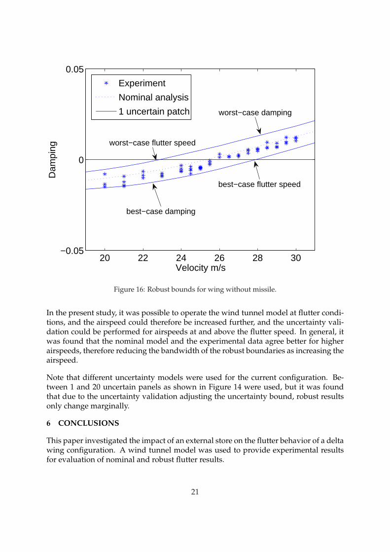
First, considering the most simple configuration without the missile (Config. 5), thevalidation was performed for one patch at a time, and it was found that the leadingedge wing tip patch introduced the most significant uncertainty. Using this patch only,an uncertainty level of 24% was required to validate the uncertain model with respectto the measured damping, which was considered to be realistic. Figure 16 shows themeasured and nominally predicted damping as a function of the velocity, as well as therobust boundaries based on the validated model. In this case, the decisive test case forthe validation bound was found to be 21 m/s, where the measured damping touchesthe robust boundary. All other experimental points are within the robust boundaries.Due to the conservative nature of the nominal model, the worst-case prediction is evenmore conservative. The validation would have produced similar results even if nodata points would have been available at and above the flutter speed. In this case, thevalidation procedure would thus be particularly useful in cases where no flutter datapoints can be collected, since the bounds established at lower airspeeds can be usedfor robust analysis at higher speeds.

Another approach is be to increase the airspeed stepwise, performing an uncertaintyvalidation and predicting updated flutter bounds at every test point. Figure 17 showsresults for the configuration with the full missile, where the airspeed was increasedfrom 25 m/s up to 35 m/s. Robust boundaries were computed based on uncertaintybounds obtained from g-validation performed at each test point. Note that the nom-inally predicted flutter speed is 32 m/s and independent of any uncertainty in themodel.

Starting at 25 m/s, the uncertainty validation gives an uncertainty bound that results ina robust flutter speed between 28.6 and 35.6 m/s. In a flight test scenario where flutterconditions should be avoided, the airspeed could thus be increased to 28.6 m/s basedon the current validation. Increasing the airspeed to 26 m/s and performing anothervalidation gives new bounds for the robust flutter speed, allowing for airspeeds up to28.9 m/s. Increasing the airspeed stepwise, the lower-bound flutter speed is reachedat about 30 m/s, where both the actual testing speed and the lower-bound predictioncoincide.

20

20 22 24 26 28 30−0.05

0

0.05

Velocity m/s

Dam

ping

Experiment

Nominal analysis

1 uncertain patch

worst−case flutter speed

worst−case damping

best−case flutter speed

best−case damping

Figure 16: Robust bounds for wing without missile.

In the present study, it was possible to operate the wind tunnel model at flutter condi-tions, and the airspeed could therefore be increased further, and the uncertainty vali-dation could be performed for airspeeds at and above the flutter speed. In general, itwas found that the nominal model and the experimental data agree better for higherairspeeds, therefore reducing the bandwidth of the robust boundaries as increasing theairspeed.

Note that different uncertainty models were used for the current configuration. Be-tween 1 and 20 uncertain panels as shown in Figure 14 were used, but it was foundthat due to the uncertainty validation adjusting the uncertainty bound, robust resultsonly change marginally.

6 CONCLUSIONS

This paper investigated the impact of an external store on the flutter behavior of a deltawing configuration. A wind tunnel model was used to provide experimental resultsfor evaluation of nominal and robust flutter results.

21

24 26 28 30 32 34 36

28

29

30

31

32

33

34

35

36

Validation test speed

Flu

tter

spee

d

ExperimentNominal predictionRobust prediction

Figure 17: Robust bounds for wing with full missile.

In order to identify modeling uncertainties, it was found convenient to model the mis-sile in several steps, and to investigate how the flutter behavior changed gradually,both in the experiment and the analysis. It was found that the flutter behavior de-pends strongly on rather small missile details. This is mainly due to the location of themissile at the wing tip, where even small loads can have significant impact. Not onlythe flutter behavior as such, but also the performance and reliability of the numericalanalysis may depend on rather small details, such as the missile rear fins.

In many cases, when differences between analysis and testing are detected, finding themodeling error is rather difficult. In this study, the aerodynamic loads were assumedto be the most significant source of uncertainty, and uncertainty in the pressure coeffi-cients was introduced to account for the model imperfections. The uncertainty modelschosen in this study do not guarantee that the correct numerical model is covered bythe uncertainty description. Instead, the uncertain patches were defined by engineer-ing judgment, and the most sensitive patches selected. This selection was found toincrease the computational efficiency without compromizing the quality of the robustflutter prediction.

22

It is clear that in cases with modeling errors in the structural data, a robust approachbased on aerodynamic uncertainty may be very inefficient, since unreasonably largeuncertainty bounds may be required in order to cover these errors. For this reason, itwas here found unnecessary to adjust the uncertainty bound in order to capture thefrequency error that most likely is due to errors in the structural model.

In the present case, it was found that aerodynamic uncertainty can be used to efficientlyestablish robust flutter boundaries. Using subcritical experimental data for model val-idation, the estimated robust boundaries were found to be valid even at supercritical(unstable) conditions.

7 REFERENCES

[1] D. Borglund. The µ-k Method for Robust Flutter Solutions. AIAA Journal of Air-craft, 41(5):1209–1216, 2004.

[2] D. Borglund and U. Ringertz. Efficient Computation of Robust Flutter BoundariesUsing the µ-k Method. AIAA Journal of Aircraft, 43(6):1763–1769, 2006.

[3] S. Heinze and D. Borglund. Robust Flutter Analysis Considering Modeshape Vari-ations. Technical Report TRITA-AVE 2007:27, Department of Aeronautical andVehicle Engineering, KTH, 2007. Submitted for publication.

[4] B. Moulin. Modeling of Aeroservoelastic Systems with Structural and Aerody-namic Variations. AIAA Journal, 43(12):2503–2513, 2005.

[5] MSC Software Corporation, Santa Ana, California. Nastran Reference Manual, 2004.

[6] Zona Technology, Scottsdale, Arizona. ZAERO Applications Manual, Version 7.1,2004.

[7] E. Albano and W. P. Rodden. A Doublet-Lattice Method for Calculating Lift Dis-tributions on Oscillating Surfaces in Subsonic Flows. AIAA Journal, 7(2):279–285,1969.

[8] D. Borglund. Robust Aeroelastic Analysis in the Laplace Domain: The µ-pMethod. In CEAS/AIAA/KTH International Forum on Aeroelasticity and StructuralDynamics, Stockholm, Sweden, June 2007.

[9] D. Borglund. Upper Bound Flutter Speed Estimation Using the µ-k Method. AIAAJournal of Aircraft, 42(2):555–557, 2005.

[10] K. Zhou and J. C. Doyle. Essentials of Robust Control. Prentice-Hall, Upper SaddleRiver, NJ, 1998.

[11] G. J. Balas, J. C. Doyle, K. Glover, A. Packard, and R. Smith. µ-Analysis and Syn-thesis TOOLBOX for Use with MATLAB. The MathWorks, Inc., Natick, MA, 1995.

23