on the road to prosperity?
TRANSCRIPT
Policy Research Working Paper 5479
On the Road to Prosperity?
The Economic Geography of China’s National Expressway Network
Mark RobertsUwe DeichmannBernard Fingleton
Tuo Shi
The World BankDevelopment Research GroupEnvironment and Energy TeamNovember 2010
WPS5479P
ublic
Dis
clos
ure
Aut
horiz
edP
ublic
Dis
clos
ure
Aut
horiz
edP
ublic
Dis
clos
ure
Aut
horiz
edP
ublic
Dis
clos
ure
Aut
horiz
edP
ublic
Dis
clos
ure
Aut
horiz
edP
ublic
Dis
clos
ure
Aut
horiz
edP
ublic
Dis
clos
ure
Aut
horiz
edP
ublic
Dis
clos
ure
Aut
horiz
ed

Produced by the Research Support Team
Abstract
The Policy Research Working Paper Series disseminates the findings of work in progress to encourage the exchange of ideas about development issues. An objective of the series is to get the findings out quickly, even if the presentations are less than fully polished. The papers carry the names of the authors and should be cited accordingly. The findings, interpretations, and conclusions expressed in this paper are entirely those of the authors. They do not necessarily represent the views of the International Bank for Reconstruction and Development/World Bank and its affiliated organizations, or those of the Executive Directors of the World Bank or the governments they represent.
Policy Research Working Paper 5479
Over the past two decades, China has embarked on an ambitious program of expressway network expansion. By facilitating market integration, this program aims both to promote efficiency at the national level and to contribute to the catch-up of lagging inland regions with prosperous Eastern ones. This paper evaluates the aggregate and spatial economic impacts of China’s newly constructed National Expressway Network, focussing, in particular, on its short-run impacts. To achieve this aim, the authors adopt a counterfactual approach based on the estimation and simulation of a structural “new economic geography”
This paper—a product of the Environment and Energy Team, Development Research Group—is part of a larger effort in the department to better understand the benefits of infrastructure investments for development. Policy Research Working Papers are also posted on the Web at http://econ.worldbank.org. The authors may be contacted at [email protected], [email protected], [email protected] and [email protected].
model. Overall, they find that aggregate Chinese real income was approximately 6 percent higher than it would have been in 2007 had the expressway network not been built. Although there is considerable heterogeneity in the results, the authors do not find evidence of a significant reduction in disparities across prefectural level regions or of a reduction in urban-rural disparities. If anything, the expressway network appears to have reinforced existing patterns of spatial inequality, although, over time, these will likely be reduced by enhanced migration.
On the road to prosperity? The economic geography of
China's national expressway network
Mark Roberts1, Uwe Deichmann2, Bernard Fingleton3 and Tuo Shi1
1 Department of Land Economy, University of Cambridge 2 Development Research Group, World Bank
3 Department of Economics, University of Strathclyde
* The research presented in this paper has been supported by the Research Support Budget of the World Bank. The authors would like to thank Harry Garretsen and Andreas Kopp for useful discussions during the research undertaken for this paper, as well as Ede Jorge Ijjasz-Vasquez, Louis Kuijs, John Scales and other members of the World Bank's China Transport Team for useful feedback on an earlier draft. The findings, interpretations, and conclusions expressed in this paper are entirely those of the authors. They do not necessarily represent the views of the International Bank for Reconstruction and Development/World Bank and its affiliated organizations, or those of the Executive Directors of the World Bank or the governments they represent.
2
1. Introduction
Between 1990 and 2005, China invested approximately US$600 billion, or US$40 billion per
annum, to upgrade its road system. The centerpiece of this massive infrastructure program
was the building of a 41,000 km National Expressway Network (NEN; World Bank 2007).1
This highway network, which is second in length only to the US Interstate Highway System2,
is designed to eventually connect all cities of more than 200,000 people and its construction
has formed an important part of China's national development strategy. Along with trade
facilitation, one of its goals, therefore, has been to promote the faster development of China's
poorer inland regions, thereby assisting in their catch-up with more prosperous coastal areas.3
This aim has come to be seen as increasingly pressing in Chinese policy discourse in light of
wide, and growing, regional disparities. In 2007, the GDP per capita of China's richest
prefectural-level region (Dongying City) exceeded that of its poorest (Hotan Prefecuture) by
a factor of more than 24:1. To put this into perspective, this is roughly equal to the ratio of
the United States' GDP per capita to that of Cameroon's.
In this paper, we present a short-run analysis of both the national and spatial economic
impacts of China's NEN. We assess not only how this massive investment program has
affected regional disparities, but also disparities between urban and rural areas, which are
also a prominent concern in Chinese policy debates (Meng et al. 2005; Ravallion and Chen
2007; Hering and Poncet 2010a). The rationale behind large-scale transport investments
between leading and lagging regions is usually to encourage the de-concentration of
economic activity. Improved infrastructure lowers transport costs and thereby promotes
integration of the national market. This enables producers and consumers in remote areas to
gain better access to prosperous urban markets and lower prices for inputs and goods.
However, producers in leading areas also benefit from falling transport costs. As their market
reach increases, they achieve even greater scale economies, lowering costs and increasing
competitiveness. So, a priori it is not entirely clear where the gains from infrastructure
1 Expansion of the network has since continued, with its current length standing at around 65,000 km (according to the National Bureau of Statistics, China). 2 For comparison, the total network length of the US Interstate Highway System is 75,000 km (http://www.fhwa.dot.gov/interstate/faq.htm#question3). 3 "In the light of the national development strategy, planning and building a national expressway network will facilitate the establishment of a unified market in the country, thus promoting commodities and various other resources to flow and compete freely around the country, which is of great importance in narrowing down the development gaps between different regions, increasing job opportunities and pushing the development of related industries. Based on a summary of the experiences of economic and social development in the developed countries, the national expressway network plan is an urgent need for the building of an all-round well-off society and for the realization of modernization…" (http://www.crcc.cn/536-1712-4102.aspx).
3
investments will be greatest. This is particularly so for labor in the short-run, before
migration has had the opportunity to arbitrage away spatial real wage differentials associated
with geographical asymmetries in market access. A better understanding of these dynamics
would help policy makers anticipate geographically differentiated impacts from road
investments. For instance, if better connectivity widens disparities in the short-run, the
additional induced migration to leading urban areas that might be expected to occur in the
long-run will accelerate demand for housing and public services in those areas.
The New Economic Geography (NEG) framework pioneered by Krugman and various co-
authors (Krugman, 1991a, 1991b; Fujita et al., 1999) provides a suitable starting point to
address these questions. Unlike earlier theoretical paradigms, these models enable explicit
microeconomic assumptions to coexist alongside increasing returns to scale within a general
equilibrium framework (Ottaviano and Thisse, 2004). This seamless theoretical integration
has enhanced the attractiveness of NEG models among the wider economics profession, and
provides us with a theoretically and empirically coherent way to explore research questions
relating to the spatial impacts of major interregional transport projects. The key idea that is
central to the NEG is the notion that transport costs affect economic outcomes. This is not a
new idea of course (see, for example, Ottaviano and Thisse, 2004, on this point), but the NEG
provides a rigorous framework for empirical modeling and enforces internal consistency. As
explained in detail below, we measure transport cost changes (as reflected in reduced travel
times) due to China's investment in the NEN using Geographic Information Systems (GIS)
methods. This produces changes in economic outcomes under the theoretical and empirical
model. We focus on the short-run equilibrium outcomes of the NEG model, rather than long-
run outcomes. The latter would require an analysis of migration in response to real wage
disparities, which, although undoubtedly important to a complete assessment of the NEN's
eventual impacts, is beyond the scope of the current paper.4
The theoretical relationship between wages and "market access" – the so-called NEG wage
equation – lies at the core of our analysis. This builds on the now well-established literature
which estimates the wage equation (see, inter alia, Hanson, 1997, 2005; Redding and
Venables, 2004; Brakman et al, 2006; Fingleton, 2005a, 2006, 2008; Fischer and Fingleton,
4 It may also be argued that, from a spatial perspective, the short-run impacts are the more interesting. In the long-run, it is obvious that labor mobility will help to erode any short-run changes in regional and/or urban-rural disparities induced by a change in transport costs. By contrast, the short-run impacts on spatial and urban-rural inequalities are theoretically ambiguous as to their direction. Furthermore, modelling the short-run impacts is a prerequisite for modelling the long-run impacts. Finally, the short-run may last many years or even decades.

4
2009), but it has a number of innovative aspects. First, unlike most NEG applications,
including applications to China (see, for example, Au and Henderson, 2006; Moreno-Monroy,
2008; Bosker et al, 2010; Hering and Poncet, 2010a, 2010b), it allows sectoral
disaggregation; in our case, we disaggregate the regions of analysis into urban and rural
sectors. Second, this paper is one of the first to use the full set of structural equations from an
NEG model for the explicit purpose of applied policy evaluation (for a similar application to
the reform of China’s Hukou system see Bosker et al, 2010). Third, while most empirical
NEG applications use a simplified measure of transport costs – such as straight line distance
– we utilize detailed GIS-derived data on a country's road network to derive travel time
estimates that can be shown to relate closely with transport costs (see Combes and
Lafourcade, 2005; Bröcker, 2002). Our travel time estimates are taken from a detailed digital
representation of China's road network with and without the NEN.5
Building on earlier work by Fujita et al. (1999, chp. 7) and Fingleton (2005b, 2007), we
develop a two-sector, multi-region, NEG model of the Chinese economy based on 331
prefectural level regions (prefectures for brevity) spread over the entire territory of China.6
Prefectures are typically large and varied, so that each contains both an urban and a rural
economy. The urban-rural distinction in China is fundamental to understanding the Chinese
economy and this distinction is reflected in our impact measures, which are aggregate real
income together with real urban wages and real rural wages. As noted above, an important
variable in the set of equations leading to the short-run equilibrium of the NEG model is the
concept of "market access" or "market potential." A prefecture with strong market access
will, typically, possess pecuniary externalities which will tend to enhance wage levels.
Fundamentally, market access is shaped by transport costs. We compute the changes in
estimated travel times between each pair of prefectures as the basis for calculating transport
cost, and, therefore, market access, changes.
NEN impact evaluation is constrained by necessary trade-offs between geographic specificity
and data availability. Since consistent time series data for our impact measures and other
relevant variables are not available for a geographically comprehensive sample of prefectures,
and because the NEN can be expected to have had substantial spatial general equilibrium
effects which might otherwise be difficult to capture, we adopt a counterfactual approach.
5 The data set and the construction of our GIS road networks data are discussed in more detail in Appendix A. 6 Our analysis focuses only on mainland China. The only province not included is Tibet. This is because of data constraints.
5
First, we estimate the key parameters of our NEG model using detailed data for 2007 and
market access based on the road network that includes the NEN. The equilibrium solution of
this model provides an accurate empirical description of the observed spatial distribution of
income and wage levels. We then use this model to simulate the (real) income and wage
levels which would have existed in 2007 had the NEN not been constructed – that is, the
spatial distribution of our outcome measures if market access had not been significantly
improved. By comparing these income levels with those under our original equilibrium
solution we arrive at estimates of the short-run impacts of the NEN up to 2007.7
Given an explicit NEG general equilibrium framework, we are able to fully capture the
impacts of the NEN road network expansion, the totality of which would be missed by other
impact evaluation approaches. Under the model, improving a link in a road network not only
benefits the immediate vicinity, but also areas further away whose trade and travel passes
through that link. Better transport infrastructure thus changes the relative strength of
agglomeration and dispersion forces in the entire country. This shapes the geography of
market access and consequently the spatial distribution of wage and income levels. Moreover,
our NEG model incorporates the full set of price changes resulting from transport cost
reductions, so that we can measure both nominal and real quantities, for instance real urban
wages. However, we enhance the theoretical NEG model, in which wages are determined
solely by market access via the wage equation, by also allowing for (empirically estimated)
variations in the efficiency of labor both across prefectures and between the urban and rural
sectors.
Our results suggest that Chinese real income in 2007 was approximately 6 percent higher
than it would have been, had the NEN not been built. As already indicated, this is a short-run
estimate that does not take into account possible additional effects associated with the long-
run mobility of labor. It is also a one-off level effect, as opposed to a permanent growth rate
effect, as a result of a boost to productivity levels. The estimated impacts of China's NEN
investments vary both across prefectures and between urban and rural areas. In all but one
prefecture, overall estimated real income has increased.8 The largest real income gains,
however, have been concentrated in the East of China, so that, contrary to its objectives, the
NEN has, thus far, done little to alleviate disparities between the coastal and interior 7 Our estimates of impact exclude those (temporary) impacts associated with the actual construction of the NEN itself (e.g., employment of construction workers). 8 The exception is Changji Hui Autonomous Prefecture, located in north-eastern Xinjiang. But the decline in real income is only 0.53 percent.
6
prefectures. Across sectors, the picture is more differentiated. In about one-third of
prefectures, either the rural or urban sector has experienced a decline in real wages. Typically,
real wage increases attributable to the NEN have been negatively correlated across the urban
and rural sectors, which is consistent with a pattern of increased specialization. Finally, the
NEN has had little impact on reducing the level and dispersion of urban-rural income
disparities across prefectures – for example, the mean urban-rural wage ratio across
prefectures in 2007 is virtually identical to what it would have been in the absence of the
NEN.
The structure of the remainder of the paper is as follows. Section 2 provides a short review
of alternative approaches to the impact evaluation of large-scale interregional transport
projects. Section 3 outlines both our theoretical model and our methodology for obtaining
estimates of impacts using this model. Section 4 discusses in greater detail the estimation of
the wage equations for the urban and rural sectors of the Chinese economy, which provides
an important intermediate step in our methodology, and reports associated results. Section 5
reports our final results for the aggregate and spatial economic impacts of the NEN. Finally,
section 6 concludes.
2. Approaches to Impact Assessment of Transport Sector Investments
There are two commonly used approaches for assessing the impacts of large-scale inter-
regional transport infrastructure projects – operational cost benefit analysis (CBA) and
macro-level empirical analysis. Standard CBA focuses exclusively on the transport market. It
estimates project benefits through anticipated reductions in travel time, vehicle operating
costs and transport related accidents. In the absence of externalities or market imperfections,
transport economics shows that such benefits accurately capture total project benefits
(Wheaton, 1977; see also Vickerman, 2000; Laird et al., 2005). Other benefits, such as rising
land values, are considered reflections of the transport benefits in other markets rather than
distinct (World Bank, 2006, pp 2-3). CBA is a tried and tested approach and relatively easy
to apply. Consequently, at a policy level, it constitutes the standard approach towards ex ante
assessment of benefits, especially at the level of individual projects. However, this approach
does not capture additional indirect benefits of travel time reductions induced by a project,
which may include economic gains outside the actual project area.

7
The macro level empirical literature seeks to establish social rates of return to infrastructure
investment, for example, by estimating aggregate production functions in which
infrastructure is a factor. This approach can capture additional positive externalities,
including those associated with NEG-style forces. Ever since Aschauer (1989) reported
extremely large estimated elasticities of output with respect to public capital, this literature
has been viewed critically, in part because of endogeneity and measurement problems. The
recent review and meta-analysis by Straub (2008) highlights the considerable empirical
uncertainty of the productivity and growth effects of infrastructure across studies using a
wide range of samples, time periods and methods. This is illustrated by research on the
impacts of the U.S. interstate highway system, constructed between 1956 and about 1973,
which, in many ways, resembles China’s NEN. Most studies look at impacts in specific
sectors or regions. Keeler and Ying (1988) use a cost function approach and estimate benefits
for the road freight transport industry that alone justify between one-third and one-half of the
cost of the system. But they also find that after the early 1970s, the marginal benefits of
additional highway investments were close to zero. Fernald (1999) confirms this finding in a
study of the system's effect on total factor productivity (TFP). He estimates sector specific
production functions that suggest the interstate system contributed about one additional
percentage point to TFP growth before 1973. After completion of the program, the system did
not contribute significantly to further productivity growth.
Chandra and Thompson (2000) focus on non-metropolitan counties where they estimate a
cumulative growth premium of 6-8 percent in counties traversed by a highway, but a
reduction in adjacent counties of 1-3 percent. This suggests that some of the rural benefits
come from relocated, as opposed to newly created, economic activity. Michaels (2008)
assumes that highways increased trade related activities in rural counties, which raised
demand for skilled manufacturing workers in skill-abundant counties and reduced it in others.
This increased trucking income and retail sales by about 7-10 percent per capita in rural
counties crossed by highways relative to other counties. Finally, Shirley and Winston (2004)
focus on another specific mechanism by which highways affect economic growth: reductions
in inventories and thus logistics costs. They find significant annual rates of return that
reached more than 17 percent in the 1970s, but then fell to less than 5 percent in the 1980s
and about 1 percent in the 1990s.
8
Impact evaluation approaches based on the new economic geography (NEG) provide an
alternative framework for infrastructure impact evaluation. The NEG aims to model the
interplay between the agglomeration and dispersion forces that shape the spatial distribution
of economic outcomes. Building on a long tradition in economic geography, the NEG has
developed models that integrate location dynamics within a general equilibrium framework
explicitly accounting for transport costs (Ottaviano and Thisse, 2004). Within NEG theory,
declining transport costs change the relative strength of forces leading to concentration or
dispersal of economic activity. In many NEG models, a reduction in transport costs at first
promotes widening regional disparities and an increased agglomeration of activity before
eventually inducing convergence and a dispersion of activity when congestion costs outweigh
transport cost savings (see Puga, 2002, for a discussion – particularly pp 387-390).9 For a
given level of agricultural transport costs, this is also the predicted relationship between
manufacturing transport costs and the spatial distribution of activity in the two region version
of the model in Fujita et al. (1999, ch. 7) that we modify and generalize in our application to
China.
Like other approaches, NEG models reflect compromises in representing the real economy
(e.g., Martin, 1999; Neary, 2001). But the NEG approach has three main advantages in the
evaluation of transport investment impacts. First, as already stated, it captures spatial general
equilibrium effects associated with the changing strength of agglomeration and dispersion
forces. Second, because it is founded on an explicit spatial general equilibrium framework, it
links the potential impacts of projects to key structural characteristics of an economy, such as
the existing level of transport costs in different sectors, the relative importance of sectors
characterized by increasing returns to scale, and the degree of factor mobility – and, therefore,
the size and extent of policy and institutional barriers on labor mobility, such as those
associated with the permanent household registration, i.e. Hukou, system in China. An NEG-
based approach captures heterogeneous impacts of projects across geographic areas and time,
which can help explain the seemingly contradictory results in the macro level empirical
literature. Finally, an NEG-based approach can, potentially, capture both the short- and long-
run aggregate and spatial economic impacts of a project. We may associate short-run impacts
with a fixed spatial and sectoral distribution of employment and long-run impacts with
additional effects emanating from labor mobility and migration. This helps identify a variable
9 This bell-shaped relationship between transport costs and the level of agglomeration is to be contrasted with the simpler "tomahawk" relationship predicted by the original Krugman (1991a, 1991b) model.

9
time-profile of impacts on, for example, inequalities between leading and lagging regions.
Investments could initially increase inequality in real wages between regions, but labor
mobility will then eventually arbitrage away such (cost-of-living adjusted) differences.
Simulating the long-run equilibrium does, however, introduce an extra layer of complexity,
not least because of the crudeness of the modeling of migration decisions in NEG theory to
date. It is for this reason, as stated before, that we focus only on short-run impacts in our
application to China.
Initial transport impact assessments built on elements of NEG theory took the form of Spatial
Computable General Equilibrium (SCGE) models. For instance, the EU's CGEurope model
has been developed to assess the impacts of proposed Trans-European Transport Network
(TEN-T) projects to better connect lagging European regions with leading ones.10 Further
examples include the RAEM model for the Netherlands for ex ante assessment of proposed
magnetic levitation rail projects (Oosterhaven and Elhorst, 2008). Our approach instead
builds more directly on the academic empirical NEG literature which estimates the so-called
NEG wage equation – the predicted relationship between nominal wages and a measure of a
region's market access (Au and Henderson, 2006; Bosker et al., 2010; Brakman et al, 2006;
Hering and Poncet, 2010a, 2010b). Other closely related work uses a full structural NEG
model to simulate the short-run spatial economic impacts of a generalized reduction in
transport costs. This reduction is modeled as a change in a scalar parameter which enters into
a transport cost function based on straight-line distance (Brakman et al., 2006; Fingleton,
2005b, 2007).
3. Theory and Strategy for Estimating Impacts
3.1. The Model11
The theoretical model which underpins our approach is a development of the basic two sector
NEG model (Krugman, 1991a, 1991b) that accommodates explicitly defined transport costs
and the extension of Dixit-Stiglitz "love of variety" preferences (and, therefore, product
differentiation) to both sectors, as set out by Fujita et al. (1999, chp. 7) and Fingleton (2005b,
10 These include its IASON (Integrated Appraisal of Spatial Effects of Transport Investments and Policies) project, its EPSON (European Spatial Planning Observation Network) Territorial Impact of EU Transport and TEN Policies project, and its ASSESS report. For an overview of the theory underlying this model see Bröcker (2002). 11 Given that the basic structure of NEG models is now very well-known (see, for example, the detailed textbook overviews provided by Fujita et al., 1999, and Brakman et al., 2009), we do not provide a detailed technical overview of our model in this section.
10
2007). In addition, in the interest of greater realism, the model is written in terms of labor
efficiency units rather than the labor units which typify the early versions of NEG theory. We
allow labor efficiency to vary both across regions and sectors, building on Fujita et. al., (1999,
chp. 15) and Südekum (2005). The urban sector is assumed to comprise production units
characterized by internal economies of scale with a market structure typified by monopolistic
competition. In contrast, the rural sector has production units with constant returns to scale
under perfect competition. This urban-rural differentiation is adopted in place of the
manufacturing-agricultural dichotomy common to NEG models because it is more
appropriate to the Chinese situation, where we are more likely to see increasing returns in the
urban economy, and it provides more amenable data. Relative to Krugman (1991a, b), the
extension of transport costs and "love of variety" preferences to the rural sector introduces an
additional dispersion force, which offsets the well-known agglomeration bias of the original
Krugman model (Fujita et al., 1999, chp. 7). Meanwhile, allowing labor efficiency to vary
both across regions and sectors permits for the incorporation of non-NEG forces.
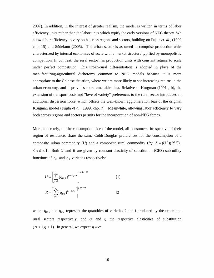
More concretely, on the consumption side of the model, all consumers, irrespective of their
region of residence, share the same Cobb-Douglas preferences for the consumption of a
composite urban commodity (U) and a composite rural commodity (R): ))(( 1 RUZ ,
10 . Both U and R are given by constant elasticity of substitution (CES) sub-utility
functions of Un and Rn varieties respectively:
)1/(
1
/)1(, )(
Un
kkUqU [1]
)1/(
/)1(
1, )(
Rn
llRqR [2]
where kUq , and lRq , represent the quantities of varieties k and l produced by the urban and
rural sectors respectively, and and the respective elasticities of substitution
( 1,1 ). In general, we expect .
11
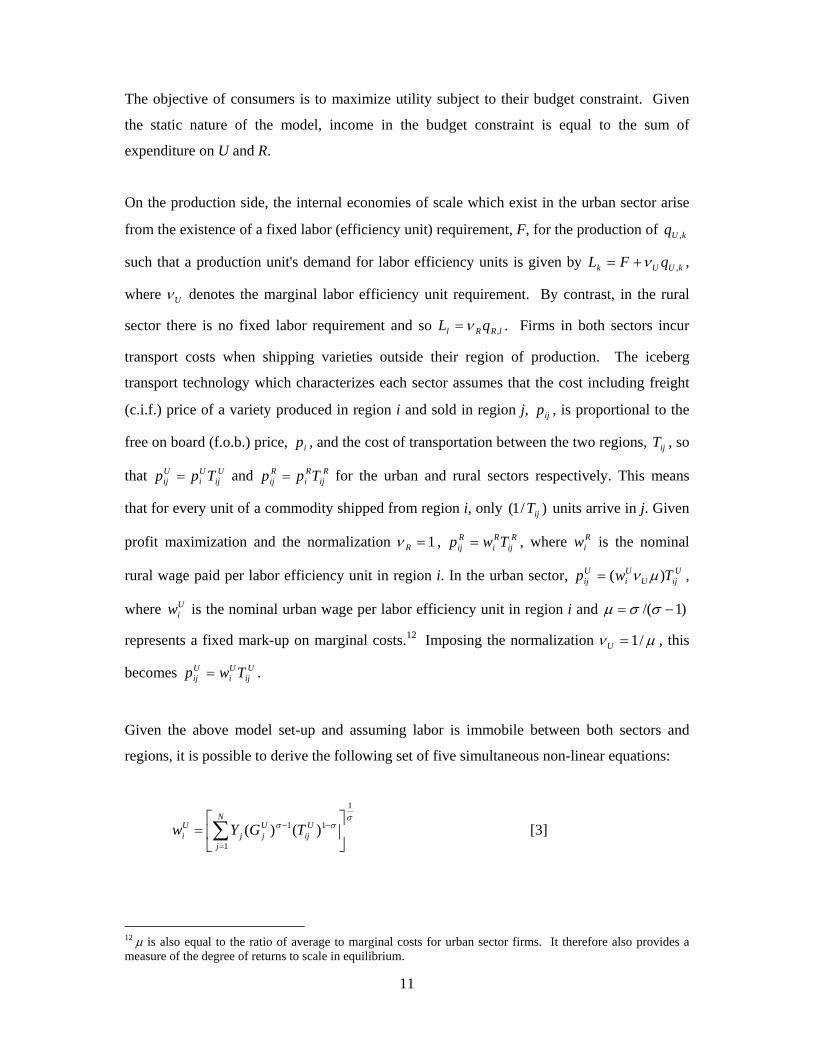
The objective of consumers is to maximize utility subject to their budget constraint. Given
the static nature of the model, income in the budget constraint is equal to the sum of
expenditure on U and R.
On the production side, the internal economies of scale which exist in the urban sector arise
from the existence of a fixed labor (efficiency unit) requirement, F, for the production of kUq ,
such that a production unit's demand for labor efficiency units is given by kUUk qFL , ,
where U denotes the marginal labor efficiency unit requirement. By contrast, in the rural
sector there is no fixed labor requirement and so lRRl qL , . Firms in both sectors incur
transport costs when shipping varieties outside their region of production. The iceberg
transport technology which characterizes each sector assumes that the cost including freight
(c.i.f.) price of a variety produced in region i and sold in region j, ijp , is proportional to the
free on board (f.o.b.) price, ip , and the cost of transportation between the two regions, ijT , so
that Uij
Ui
Uij Tpp and R
ijRi
Rij Tpp for the urban and rural sectors respectively. This means
that for every unit of a commodity shipped from region i, only )/1( ijT units arrive in j. Given
profit maximization and the normalization 1R , Rij
Ri
Rij Twp , where R
iw is the nominal
rural wage paid per labor efficiency unit in region i. In the urban sector, UijU
Ui
Uij Twp )( ,
where Uiw is the nominal urban wage per labor efficiency unit in region i and )1/(
represents a fixed mark-up on marginal costs.12 Imposing the normalization /1U , this
becomes Uij
Ui
Uij Twp .
Given the above model set-up and assuming labor is immobile between both sectors and
regions, it is possible to derive the following set of five simultaneous non-linear equations:
1
1 1
1
( ) ( )N
U U Ui j j ij
j
w Y G T
[3]
12 is also equal to the ratio of average to marginal costs for urban sector firms. It therefore also provides a measure of the degree of returns to scale in equilibrium.

12
1
11
1
)()(
R
ijRj
N
jj
Ri TGYw [4]
1
1
1
1)(N
j
Uij
Ujj
Uj
Ui TwG [5]
1
1
1
1)(N
j
Rij
Rjj
Rj
Ri TwG [6]
Rii
Ri
Uii
Uii wwY )1( [7]
In these equations, iUi is the number of urban labor efficiency units in region i, equal to the
product of labor efficiency Uj and labor units i . Likewise, i
Ri is the number of rural
labor efficiency units in region i, equal to the product of rural labor efficiency Ri and rural
labor units i . Also, Uiw is the urban wage rate per efficiency unit of labor and R
iw is the
rural wage rate per efficiency unit of labor, UiG and R
iG are the respective price indices, and
iY is the income level, which is equal to the weighted sum of the number of efficiency units
iUi times the efficiency unit wage rate U
iw for the urban economy, and rural efficiency
units iRi times rural efficiency unit wages R
iw . The weights and 1 are approximated
by the respective urban and rural shares of total employment in the Chinese economy.
Taken together, these equations describe the short-run equilibrium solution for a given region
1,..., .i N In equations [3] and [4], we have the wage equations as they apply to the urban
and rural sectors, and expressed in terms of wages per labor efficiency unit. The terms in the
square brackets on the right hand side of equations [3] and [4] are the real "market access"
(RMA) levels for region i; they are real because of the presence of the price indices UiG and
RiG . From an impact evaluation viewpoint however, we are more interested in wages per
worker, which we denote by *Uiw and *R
iw respectively. We, therefore, convert to (nominal)
wages by scaling by efficiency levels. For any given number of labor efficiency units, the
wage per unit of labor will be higher for a small number of efficient workers than if the
number of labor efficiency units comprises a large number of inefficient workers. Therefore,
the wage per worker is the wage per efficiency unit times the efficiency level. For example,
13
if wages are US$100 per labor efficiency unit, and we have 100 labor efficiency units
because we have two workers and an efficiency level of 50, then the wage per worker is
US$5000. With 100 workers at efficiency level 1, the wage per worker is US$100. Equations
[3] and [4] may thus be re-written as * 1/( )U U U U Ui i i i iw w RMA and * 1/( )R R R
i i iw RMA
respectively, where UiRMA denotes region i's level of RMA in the urban sector and R
iRMA its
level of RMA in the rural sector. UiRMA is basically equal to the weighted sum of real
aggregate income levels across all regions, including region i, where the weights are
determined by the cost of transporting urban goods from i to each region. Ceteris paribus,
UiRMA can therefore be expected to increase if real incomes in surrounding regions increase
or if costs of transportation fall. Regions with high levels of nominal urban wages will be
those which are well-connected to other regions which have high levels of real income. A
similar interpretation applies to RiRMA except that it is the cost of transporting rural goods
from i to each region which is now important.
Efficiency levels are defined relative to the minimum observed level of labor efficiency in the
urban sector. Hence, for the urban sector, UUi
Ui AA min/ , whilst, for the rural sector,
URi
Ri AA min/ , where iA denotes a region's absolute level of labor efficiency and U
iA the
minimum observed level of labor efficiency in the urban sector. The presence of these
parameters in equations [3] and [4] imply that non-NEG, as well as NEG, forces will be
important in determining the geography of both urban and rural wages.
3.2. Methodology for Estimating Impacts
Our methodology consists of five stages, involving the two key wage equations – equations
[3] and [4] – and an assessment of the fit of the model's short-run equilibrium solution to
Chinese data for 2007. In the first stage, we use GIS techniques to construct two NN
travel time matrices, AfterTIME and BeforeTIME . The i-j th element of the matrix AfterTIME ,
Afterijt , measures the optimal travel time by road between regions i and j based on a digital
representation of the 2007 Chinese road network, which includes the NEN. Likewise
BeforeTIME measures optimal travel times excluding the NEN, thus providing the basis for our
counterfactual scenario. For both networks, travel time is invariant to the direction of travel,
i.e. xij
xji tt where },{ AfterBeforex . For simplicity, we also assume that 0x
iit for i . In
14
other words, that the time taken to transport goods between locations within a region is zero.
A detailed explanation of the GIS methodology used to construct both AfterTIME and
BeforeTIME is provided in Appendix A.
The second stage involves estimating the urban and rural wage equations – equations [3] and
[4] – using measures of urban and rural transport costs, UT and RT , constructed using
AfterTIME . This provides estimates of RU and ,, . In the third stage, these estimates are
used in conjunction with the actual 2007 observed values of and , to obtain a numerical
solution to equations [3] – [7], again based on AfterTIME . This solution is found through a
search procedure, which starts by assuming a set of initial values ),,,,( 00000 YGGww RURU for
Ui
Ri
Ui Gww ,, , R
iG and iY before iterating through equations [3] – [7] until convergence
between the values of these variables in successive iterations is achieved. In particular, if the
subscript m is used to denote the number of iterations, convergence is judged to have
occurred if cww mUjm
Uj 2
1 ])()[( and this is also true for UR Gw , , RG and Y, where c
is a constant which defines the tolerance condition for convergence.
The solution which results from this search procedure (which we may refer to as the "after"
solution) yields, for each region, a vector of equilibrium values ),,,( AfterAfterRAfter
UAfter Yww ,
where After = RAfter
UAfter ww / is the ratio of urban to rural wage levels. Comparing the
distributions of these values against their observed 2007 distributions provides an indication
of the "fit" of the model's equilibrium solution. The solution also yields, again, for each
region, equilibrium values for the two price indices, UAfterG and R
AfterG . These may be
combined to give a region-specific cost-of-living index, 1)()( RAfter
UAfterAfter GGP , which can
be used to derive real wage and income levels – After
RAfterR
AfterAfter
UAfterU
After P
w
P
w **
** , and
* AfterAfter
After
YY
P .
The fourth stage of the methodology is identical to the third stage, except, this time, a
numerical solution to equations [3] - [7] is obtained on the basis of measures of urban and

15
rural transport costs constructed using BeforeTIME rather than using AfterTIME . This is the
counterfactual solution. In the fifth stage, the counterfactual equilibrium values
( , , , )U RBefore Before Before Beforew w Y are deflated using the cost-of-living index,
1)()( RBefore
UBeforeBefore GGP to give the corresponding real values. These are then compared
with the corresponding "after" values to obtain estimates of impacts. To estimate the overall
impact of the NEN on aggregate Chinese nominal and real income, the results are aggregated
across regions.
3.3. Measuring Transport Costs
One crucial issue which emerges in the implementation of stages 2 – 4 is the specification of
suitable functional forms for the mapping of the travel time estimates in AfterTIME and
BeforeTIME to our measures of urban and rural transport costs, UijT and R
ijT . We assume that:
Uij
Uij tT )(10 [8]
Rij
Rij tT )(10 [9]
where 10 U and 10 R , 0 , 1 , 0 and 1 are coefficients and ijt denotes either
Afterijt or Before
ijt . Given the strong correlation which exists across prefectures between ijt and
ijd , where ijd is the straight-line distance separating the centers of regions i and j, the
concavity of transport costs implied by equations [8] and [9] is consistent with evidence from
the transport economics literature suggesting the presence of economies of distance for goods
haulage (McCann, 2005; Fingleton and McCann, 2007). A number of previous empirical
NEG studies have used the same functional form to model transport costs, including those of
Au and Henderson (2006) and Bosker et al. (2010) for China. Crucially, however, these
studies have relied on measures of Euclidean (straight-line) or great circle distance rather
than network distance or estimated travel times. But it is travel time that is most affected by
the stock and quality of transport infrastructure. Evidence of the importance of travel times
for Chinese transport costs is to be found in literature on the country's transportation and
logistics industries (see, for example, Hong et al., 2004). Meanwhile, Roberts (2010) has
demonstrated that, under reasonable conditions, travel times provide a suitable proxy for
generalized transport costs (GTCs), which capture both vehicle operating costs and the

16
opportunity cost of time. Combes and Lafourcade (2005) have also documented the
existence of a strong relationship between GTCs and estimates of optimal travel time derived
using GIS techniques for France.
4. Estimation of the Wage Equations
In this section, we discuss in detail the second stage of our methodology, the estimation of the
NEG wage equations [3] and [4]. A literature has developed following the seminal work of
Hanson (1997, 2005) and Redding and Venables (2004) which consistently finds a strong
positive relationship between RMA and nominal wages, and this has been used to provide
supporting evidence for NEG models. This includes previous work for China by, inter alia,
Au and Henderson (2006), Bosker et al. (2010), Hering and Poncet (2010a, 2010b), and
Moreno-Monroy (2008), although they typically confine themselves to the use of prefectural-
city data, whereas our sample also includes other types of prefectural-level regions (see
Appendix A). Overall, with a sample size of 331 prefectures, this makes for a more
comprehensive geographic coverage of China's territory, which is central to our purposes.
Furthermore, previous NEG wage equation studies for China have focused on the estimation
of wage equations using either aggregate data (Bosker et al., 2010; Moreno-Monroy, 2008) or
data for the urban sector only (Au and Henderson, 2006; Hering and Poncet, 2010a).
However, our theoretical model predicts that there should be a positive relationship between
RMA and nominal wages not only in the urban sector, but also in the rural sector. The
estimation of equation [4], therefore, is important for establishing the adequacy of our
underlying theoretical framework, and provides an important contribution in its own right.13
To transform equations [3] and [4] into forms that are suitable for estimation we first assume
that (relative) labor efficiency levels in both the urban and rural sectors of a region have two
components – a deterministic component and an unobservable stochastic component – so that,
for region i, iU Ui iA e and iR R
i iA e , where UA and RA denote the deterministic
components for the urban and rural sectors respectively, and and are random variates
which capture the stochastic components. Commencing with equations [3] and [4] and given
*U U Ui i iw w and *R R R
i i iw w , taking (natural) logarithms gives:
13 Without explicitly deriving it from a formal NEG model, Emran and Hou (2008) estimate a relationship between rural household consumption and measures of access to both domestic and international markets for China.
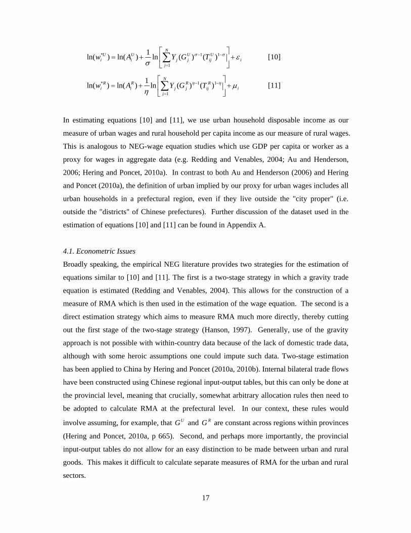
17
* 1 1
1
1ln( ) ln( ) ln ( ) ( )
NU U U U
i i j j ij ij
w A Y G T
[10]
* 1 1
1
1ln( ) ln( ) ln ( ) ( )
NR R R R
i i j j ij ij
w A Y G T
[11]
In estimating equations [10] and [11], we use urban household disposable income as our
measure of urban wages and rural household per capita income as our measure of rural wages.
This is analogous to NEG-wage equation studies which use GDP per capita or worker as a
proxy for wages in aggregate data (e.g. Redding and Venables, 2004; Au and Henderson,
2006; Hering and Poncet, 2010a). In contrast to both Au and Henderson (2006) and Hering
and Poncet (2010a), the definition of urban implied by our proxy for urban wages includes all
urban households in a prefectural region, even if they live outside the "city proper" (i.e.
outside the "districts" of Chinese prefectures). Further discussion of the dataset used in the
estimation of equations [10] and [11] can be found in Appendix A.
4.1. Econometric Issues
Broadly speaking, the empirical NEG literature provides two strategies for the estimation of
equations similar to [10] and [11]. The first is a two-stage strategy in which a gravity trade
equation is estimated (Redding and Venables, 2004). This allows for the construction of a
measure of RMA which is then used in the estimation of the wage equation. The second is a
direct estimation strategy which aims to measure RMA much more directly, thereby cutting
out the first stage of the two-stage strategy (Hanson, 1997). Generally, use of the gravity
approach is not possible with within-country data because of the lack of domestic trade data,
although with some heroic assumptions one could impute such data. Two-stage estimation
has been applied to China by Hering and Poncet (2010a, 2010b). Internal bilateral trade flows
have been constructed using Chinese regional input-output tables, but this can only be done at
the provincial level, meaning that crucially, somewhat arbitrary allocation rules then need to
be adopted to calculate RMA at the prefectural level. In our context, these rules would
involve assuming, for example, that UG and RG are constant across regions within provinces
(Hering and Poncet, 2010a, p 665). Second, and perhaps more importantly, the provincial
input-output tables do not allow for an easy distinction to be made between urban and rural
goods. This makes it difficult to calculate separate measures of RMA for the urban and rural
sectors.

18
Direct estimation of equations [10] and [11], following, inter alia, Au and Henderson (2006),
is itself problematic.14 One reason is that proxies for URMA and RRMA cannot include the
true unobserved price indices, UG and RG , and therefore previous literature has resorted to
using nominal market access (e.g. Au and Henderson, 2006), which amounts to setting
1 Ri
Ui GG for i in equations [11] and [12]; or has constructed a proxy price index
(Brakman et al., 2006; Bosker et al., 2010). The advantage of our approach is that our
structural equations [3] – [7] provide explicit expressions for UG and RG , which can be used
in their measurement. However, this still faces the difficulty that the price indices UG and
RG depend on U and R respectively, which are amongst the parameters we are seeking to
estimate as part of our wider methodology. We, therefore, assume 1U Ri i for i. We
view this as being weaker than the assumption 1 Ri
Ui GG , and crucially we control for the
measurement error thus introduced in the construction of our proxies for URMA and RRMA
through adopting an instrumental variable (IV) approach to estimation.
A second difficulty is that, as is evident from equations [3] - [7], the variables URMA , RRMA ,
together with UG and RG , embody and , which are precisely the reciprocals of the
elasticities on URMA and RRMA , parameters that we seek to estimate. One approach to this
problem following Mion (2004), Brakman et al. (2006) and Bosker et al. (2010) is the
estimation of equations [10] and [11] using non-linear least squares or non-linear 2SLS, thus
allowing the embodied and to be jointly estimated alongside the elasticities. We prefer,
however, the simpler approach of Fingleton (2005a, 2006) and, notably in a Chinese context,
Au and Henderson (2006). Our method is to assign values to and in the construction of
URMA and RRMA on the basis of past literature, and to accept these values as being
reasonable if they fall within their estimated 95 percent confidence intervals. In particular,
we assume = 3 and = 5. Albeit with a different definition of the urban sector, Au and
Henderson (2006) assume = 2 for their equivalent wage equation (p 559), and estimate =
1.5 (p. 570). These values were, however, felt to be a little on the low side in light of results
14 Some of these difficulties would also arise even if we were in a position to be able to use the two-stage strategy. In the specification of the gravity equation in the first stage of this strategy, we would still need to make assumptions about the parameters of the transport cost functions. Likewise, estimation of both the gravity equation and the final wage equations would involve dealing with problems of both simultaneity and also, potentially, spatial autocorrelation.

19
from other studies using Chinese prefectural-level data (Moreno-Monroy, 2008; Bosker et al.,
2010; Hering and Poncet, 2010a). Hence, our assumption = 3. Studies which have
estimated a prefectural-level regional wage equation for China using aggregate wage data
have obtained estimates of the elasticity of substitution in the range 5 – 8 (Moreno-Monroy,
2008, p 26; Bosker et al., 2010). Therefore, it was felt reasonable to assume = 5, on the
grounds that, a priori, we might expect there to exist more substitutability between rural
varieties than between urban varieties. Again, the possible consequence of these assumptions
is to introduce error into the measurement of URMA and RRMA , thereby further justifying
our IV approach to estimation.
Related to the above problem is the need to also specify values for the parameters 0, 1, 0,
1, U and R in the transport cost functions [8] and [9]. Again, this is necessary for the
construction of both URMA and RRMA , as well as our measures of UG and RG . Following
Fingleton (2005b, 2007), we assume 11010 so that the urban and rural
transport cost functions reduce to Uij
Uij tT )(1 and R
ijR
ij tT )(1 respectively. This still
leaves U and R as free parameters whose values need specifying. We, therefore, calibrate
these parameters, selecting values which satisfy two criteria: (a) a good fit between our
"after" model solution and actual 2007 data, and (b) satisfactory regression diagnostics,
especially relating to the validity of our instruments, for our NEG wage equations. The
values 45.0U and 75.0R satisfy (a) and (b), and imply stronger economies of
distance for urban goods transportation than for rural produced varieties.15
Our estimation of equations [10] and [11] also takes account of simultaneity and spatial
autocorrelation. Regarding simultaneity, its presence is clear from the system of structural
equations [3] – [7]. The feedback involving wages and RMA calls for an IV approach to
avoid simultaneity bias as well as solving the measurement error problem discussed above.16
15 These values seem in line with those estimated or assumed in other empirical NEG studies on China which have used a similar functional form for transport costs. Bosker et al. (2010), for example, estimate = 0.63 in assuming the functional form Tij = (dij)
, where dij measures the distance between prefectural city i and the capital of province j in their study and Tij the associated transport cost. It will be recalled that Bosker et al. estimate an aggregate wage equation and, therefore, do not distinguish between transport costs in the urban and rural sectors. 16 An IV-based approach also helps to deal with the issue of the endogenous placement of transport infrastructure. To the extent that the NEN has specifically targeted the improved connectivity of lagging (and more rural) Western regions, such endogeneity can be expected to have biased downwards the estimated co-

20
Specifically, we adopt a two-stage least squares (2SLS) approach to the estimation of both
wage equations, selecting variables which meet the requirements of valid instruments,
essentially a high level of correlation with the instrumented regressor and orthogonality with
regard to the model disturbances, for this approach.17 Failing to control for (positive) residual
spatial autocorrelation would not bias our regression estimates, but would bias inference by
downwardly biasing standard errors. We control for this by allowing for interdependencies
across regions in the determinants of labor efficiency and via the adoption of a feasible
generalized spatial two-stage least squares (FGS2SLS) estimator for both equations. This
estimator is based on the spatial General Method of Moments (GMM) estimator of Kelejian
and Prucha (1998) and is described in more detail in Fingleton and LeGallo (2008).
As specified in equations [10] and [11], our wage equations assume that China is a closed
economy. Whilst this might be acceptable for the rural sector of the Chinese economy –
agricultural and processed agricultural products, for example, accounted for only 1.4 % of
China’s exports in 200418 – it is not a reasonable assumption for the urban sector. RMA in
the urban sector of the Chinese economy is likely to have an important international
component. To deal with this, we introduce )1ln( uiportt as an additional explanatory variable
in the determination of *ln( )Uw in equation [10], where iportt denotes the optimal travel time
from region i to the nearest major international port.19 We also incorporate this variable into
our underlying theoretical model, as given by equations [3] to [7], so that, in our estimates of
impact, we are able to take account of enhancements to the international component of
URMA that have resulted from the building of the NEN. Incorporating international market
access into the theoretical model also has the effect of making the rural wage in region i
indirectly dependent on travel time to the nearest international port through our system of
structural equations.
4.2. Results
efficient of RMA in equations [10] and, in particular, [11] downwards. This is consistent with the results presented in Table 1 below for the rural wage equation, if not the urban wage equation. 17 An alternative approach, sometimes adopted in the literature, to mitigating simultaneity bias is to exclude a region's income from the calculation of its level of market access (see, for example, Mayer, 2008). 18 www.allcountries.org/china_statistics/appendix_1_16_composition_of_exports_and.html. 19 The ports which we consider in our analysis are: Shanghai, Ningbo, Tianjin, Guangzhou, Qingdao City, Dalian City, Qinhuangdao City and Shenzhen City. These correspond to the eight Chinese ports which had the largest throughput (measured in million tonnes of traffic) in ISL (2006). The first seven of these ports alone handled around 70 percent of China’s total cargo with the rest of the world in 1995 (Emran and Hou, 2008, p 16).
21
The results from the estimation of equations [10] and [11] are presented in Table 1. We have
included a number of determinants of )ln( UA and )ln( RA – namely, measures of investment
per worker (ln(I pw)) and human capital (ln(human)), as well as their "spatial lags"
(W*ln(human) and W*ln(I pw) respectively) together with Provincial level effects captured
by Provincial dummies. The spatial lag of a variable is essentially the weighted average of
that variable across neighboring prefectures. 20 Including spatial lags allows for spatial
interdependencies across regions in the determinants of levels of labor efficiency.21 However,
from a pure-NEG perspective, our main interest lies in the real market access variables –
ln(RMAdom) which captures the domestic component of RMA and )1ln( 45.0iportt which captures
the international component, which is only of direct relevance to the urban sector. Our
preferred estimates are those associated with our application of the FGS2SLS estimator. This
estimator controls both for the endogeneity of RMA and for residual spatial autocorrelation
which remains despite the inclusion of W*ln(human) and W*ln(I pw). The instruments that
we use in this estimation approach, as well as in 2SLS estimation, are the second-order
spatial lags of ln(I pw) (both wage equations) and ln(human) (only the rural wage equation),
i.e. W*W* ln(I pw) and W*W*ln(human) respectively. For the urban wage equation, we
also use a composite variable based on the Euclidean distance discounted sum of the inverse
land areas of all other prefectures as an instrument. Meanwhile, for the rural wage equation,
)1ln( 45.0iportd is used as an additional instrument, where, for a prefecture i, diport measures the
Euclidean distance to the nearest major international port. As evidenced by the first stage F-
test and Sargan test results in table 1, these variables meet the criteria for valid instruments.22
For the rural sector, our preferred FGS2SLS estimates show that the domestic component of
RMA has an important influence on nominal rural wage levels – a 10 % increase in RMAdom
increases rural wages by about 2%. This implies 887.4ˆ , which is very close to our
assumed value of 5 . Interestingly, the impact of the domestic component of RMA is
weaker for the urban sector. For this sector, a 10 % in RMAdom increases nominal urban
20 More details on all variables included in the estimation of equations [10] and [11] can be found in Appendix A. 21 They may also help us control for the possibility, identified by Emran and Hou (2008, pp 8-9), that market centers emerge in regions surrounded by areas of exceptional potential, where that potential arises from non-NEG factors. 22 Although we do not instrument the international component of market access, i.e. ln(1 + tport
0.45), in the urban wage equation in the results reported in Table 1, replacing this variable with ln(1 + dport
0.45) makes virtually no difference to the estimates obtained.
22
wages by 1.56 %. Although economically still quite strong, this estimated effect is
statistically insignificant. The implied estimate of sigma, 424.6ˆ , is greater than our
assumed value of 3 . Nevertheless, 3 is in our 95 percent confidence interval
estimate for . For the urban sector, the international component of RMA has a more potent
effect on nominal wages than the domestic component. 23 The estimated coefficient on
)1ln( 45.0iportt is strongly statistically significant, and its point estimate of -0.226 indicates, for
example, that nominal urban wages will, ceteris paribus, be 15.67 % higher in Shanghai or
Tianjin than in a region which is a one-hour drive away from an international port.
Compared to a region which is an eight-hour drive, they will be 28.63 % higher. This is
because of the favorable access to international markets which a coastal location offers.
23 These components are strongly correlated with each other - the Pearson product moment correlation coefficient is -0.7620 and the null hypothesis of no correlation can be decisively rejected.

23
Table 1: Estimation of the NEG wages equations for the urban and rural sectors, 2007
Urban Rural
Variable OLS 2SLS FGS2SLS OLS 2SLS FGS2SLS
Constant 3.042*** (3.533)
5.032*** (4.219)
3.911*** (3.892)
3.471*** (11.618)
3.564*** (11.332)
3.091*** (11.091)
ln(human) 0.565*** (7.744)
0.602*** (7.985)
0.597*** (8.135)
0.608*** (5.854)
0.431** (2.379)
0.407** (2.192)
ln(I pw) 0.107*** (5.637)
0.142*** (4.149)
0.112*** (5.876)
0.0936*** (7.877)
0.093*** (7.614)
0.090*** (7.488)
W*ln(human) -0.335*** (-2.602)
-0.281** (-2.125)
-0.279** -2.113
0.566*** (3.437)
0.530*** (3.105)
0.515*** (3.005)
W*ln(I pw) 0.148*** (4.400)
0.142*** (4.149)
0.142*** (4.102)
0.0946*** (4.662)
0.086*** (3.899)
0.077*** (3.440)
ln(RMAdom) 0.357*** (4.406)
0.136 (1.119)
0.156 (1.211)
0.139*** (8.274)
0.199*** (3.814)
0.205*** (3.770)
ln(1 + 45.0portt ) -0.190***
(-3.664) -0.251*** (-4.316)
-0.226*** (-3.820)
- - -
/ - - 0.195*** (6.890)
- - 0.164*** (7.416)
/ 2.801 7.332 6.424 7.170 5.031 4.887
2
2
R
R
2 / 2
0.766
0.739
0.017
0.760
0.732
0.017
0.771
0.744
0.015
0.859
0.842
0.026
0.853
0.836
0.028
0.856
0.839
0.024
F1st stage
Sargan, )1(2 Spatial, z-ratio
- -
6.368*** (p =0.000)
121.567*** (p = 0.000)
0.077
(p = 0.781)
3.329*** (p = 0.001)
121.567*** (p = 0.000)
0.005
(p = 0.946) -
- -
5.444*** (p =0.000)
18.038*** (p = 0.00)
0.208
(p = 0.649)
2.626*** (p = 0.009)
18.038*** (p = 0.000)
0.341
(p = 0.560) -
Notes: ***: significant at the 1 % level; **: at the 5 % level Numbers in parenthesis under parameter estimates are t-ratios F1st stage is a F-test for the joint significance of the instruments in the 1st-stage 2SLS regression. For urban, this test has (2, 294) degrees of freedom; for rural, it has (2, 295) degrees of freedom Instruments: urban – ln[j{1/[areaj(1+dij)]}], W*W*ln(I pw); rural - W*W*ln(I pw), W*W*ln(human), ln(1+diport
0.45) Sargan- statistic for Sargan's test for validity of instruments Spatial- statistic for Moran I's test for spatially autocorrelated errors (OLS) or Anselin-Kelejian (1997) test for spatially autocorrelated errors in the presence of endogenous regressors (2SLS) The 29 Provincial dummy coefficients are of limited interest and have been omitted to save space.
24
5. The Aggregate and Spatial Impacts of the NEN
5.1. Fit of "After" Equilibrium Solution
As outlined in Section 3.2, the regressions just described provide input into our full model.
Thus, we obtain our estimates of labor efficiency Uj and R
j via the regressions [10] and [11]
(Table 1), which are then a component part of our iterative solutions of equations [3] to [7].
Before we progress to discuss the estimated aggregate and spatial economic impacts from our
full model, we briefly note how well the "after" equilibrium solution to [3] – [7] describes the
distributions of key variables in 2007.24 In particular, from Appendix B, the Pearson product
moment correlation coefficients between our simulated and actual measures of (nominal)
urban and rural wages, aggregate output, and aggregate output per worker and per capita all
exceed 0.76. The strongest correlation is between our actual and simulated measures of rural
wages (r = + 0.9295), closely followed by that between our actual and simulated measures of
aggregate output (r = + 0.9212). The "after" equilibrium solution also provides a good
description of urban-rural wage ratios across prefectures. The simulated mean urban-rural
wage ratio associated with this solution is 2.961. This compares favorably with the actual
observed ratio of 2.972. The simulated standard deviation is 1.204, whilst the observed
standard deviation is 0.876. Finally, the Pearson correlation co-efficient between the
simulated and observed urban-rural wage ratios is + 0.827.
5.2. Aggregate and Spatial Impacts
At the aggregate level, the overall estimated impact of the NEN on Chinese nominal income
is 3.10 percent.25 This estimate is calculated as the percentage by which aggregate nominal
income in the "after" solution exceeds that in the "before" solution – i.e.
100]/)[(% Beforei
Beforei
Afteri
CHN YYYY , where we are summing across
prefectures. After accounting for changes in the cost-of-living across prefectures, which are
induced by the direct and indirect impacts of declining transport costs on the prices of urban
and rural varieties, our estimate of the overall impacts increases to 5.98 percent. Because we
are focussing on the short run equilibrium of the NEG model under two transport cost
24 In searching for both the "before" and "after" equilibrium solutions, we set c = 0.0001 as the tolerance condition for convergence. We also take w0
U = w0R = G0
U = G0R = Y0 = 1 as our starting values for the numerical
search procedure. 25 Given that we hold the distributions of employment fixed between the "before" and "after" scenarios, the impacts on both income per worker and per capita are identical to those for income.
25
assumptions, these estimated impacts do not take into account possible multiple equilibria
associated with the long-run dynamics resulting from the possible migration effects of the
changed geography of market access. Almost no applied work has yet been carried out on the
dynamics leading to long run equilibria, which is a topic for future research. In our model, the
response to this changed geography is assumed to manifest itself solely in prices. Our
aggregate estimates of impact also do not take into account the wage and income effects of
the expenditures on the actual construction of the NEN itself.
Despite methodological differences, our results appear to be consistent with estimates
obtained for other countries, such as the impacts of the U.S. interstate highway network. But
it should be noted that China has continued to expand the NEN since the end of 2007. It is
now almost 50 percent larger and the overall benefits due to falling transport costs and
induced effects have likely increased as well. On the other hand, studies of the U.S. network
have shown that productivity and other effects decreased significantly after the main network
had been constructed: “the interstate system was highly productive, but a second one would
not be. Road-building thus explains much of the productivity slowdown [after the 1970s]
through a one-time, unrepeatable productivity boost in the 1950s and 1960s" (Fernald, 1999,
p 619). This raises the question whether NEN benefits might reach a peak once a saturation
point in terms of highway coverage has been reached. Whether China – the world’s 3rd
largest country with the largest population – has reached this point is an interesting question
for further research.
We have shown a sizeable overall impact due to the NEN. Looking at the picture across
prefectures, the mean increase in real income is 3.95 percent compared to a median increase
of 3.13 percent, indicating that the distribution of gains has been positively skewed. This
reflects the fact that the largest real income gains have been concentrated in the east of China
(Figure 1). This is consistent with the statistically significant positive relationship between a
region's level of real income per worker in the "before" scenario and the percentage change in
real income per worker attributed to the NEN (Figure 1).26 This suggests that the building of
the NEN may have at least initially increased divergence between regions rather than
promoted the intended convergence. The standard deviation of the log of real income per
worker also shows barely any change between the "before" and "after" scenarios (0.397
26 The estimated slope coefficient for the OLS regression line shown in Figure 2 is 2.749 and the associated t-statistic is 10.327. R2 = 0.245. The classification of prefectures into macro-regions in Figure 2 is the same as that used in the ANOVA exercise in Appendix C.
26
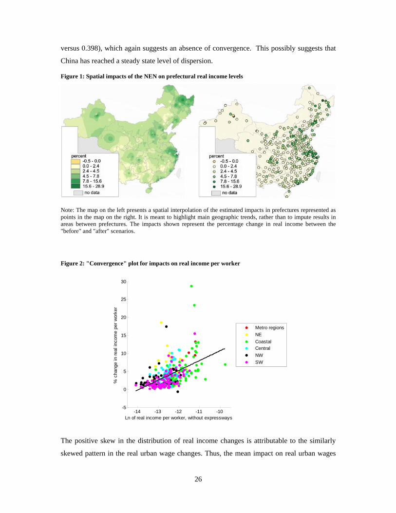
versus 0.398), which again suggests an absence of convergence. This possibly suggests that
China has reached a steady state level of dispersion.
Figure 1: Spatial impacts of the NEN on prefectural real income levels
Note: The map on the left presents a spatial interpolation of the estimated impacts in prefectures represented as points in the map on the right. It is meant to highlight main geographic trends, rather than to impute results in areas between prefectures. The impacts shown represent the percentage change in real income between the "before" and "after" scenarios.
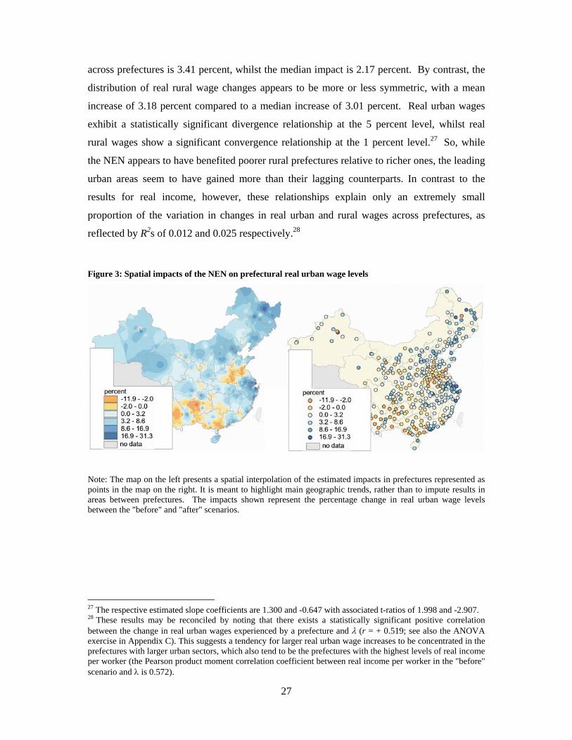
Figure 2: "Convergence" plot for impacts on real income per worker
-14 -13 -12 -11 -10-5
0
5
10
15
20
25
30
% c
hang
e in
rea
l inc
ome
per
wor
ker
Ln of real income per worker, without expressways
Metro regions
NE
CoastalCentral
NW
SW
The positive skew in the distribution of real income changes is attributable to the similarly
skewed pattern in the real urban wage changes. Thus, the mean impact on real urban wages
27
across prefectures is 3.41 percent, whilst the median impact is 2.17 percent. By contrast, the
distribution of real rural wage changes appears to be more or less symmetric, with a mean
increase of 3.18 percent compared to a median increase of 3.01 percent. Real urban wages
exhibit a statistically significant divergence relationship at the 5 percent level, whilst real
rural wages show a significant convergence relationship at the 1 percent level.27 So, while
the NEN appears to have benefited poorer rural prefectures relative to richer ones, the leading
urban areas seem to have gained more than their lagging counterparts. In contrast to the
results for real income, however, these relationships explain only an extremely small
proportion of the variation in changes in real urban and rural wages across prefectures, as
reflected by R2s of 0.012 and 0.025 respectively.28
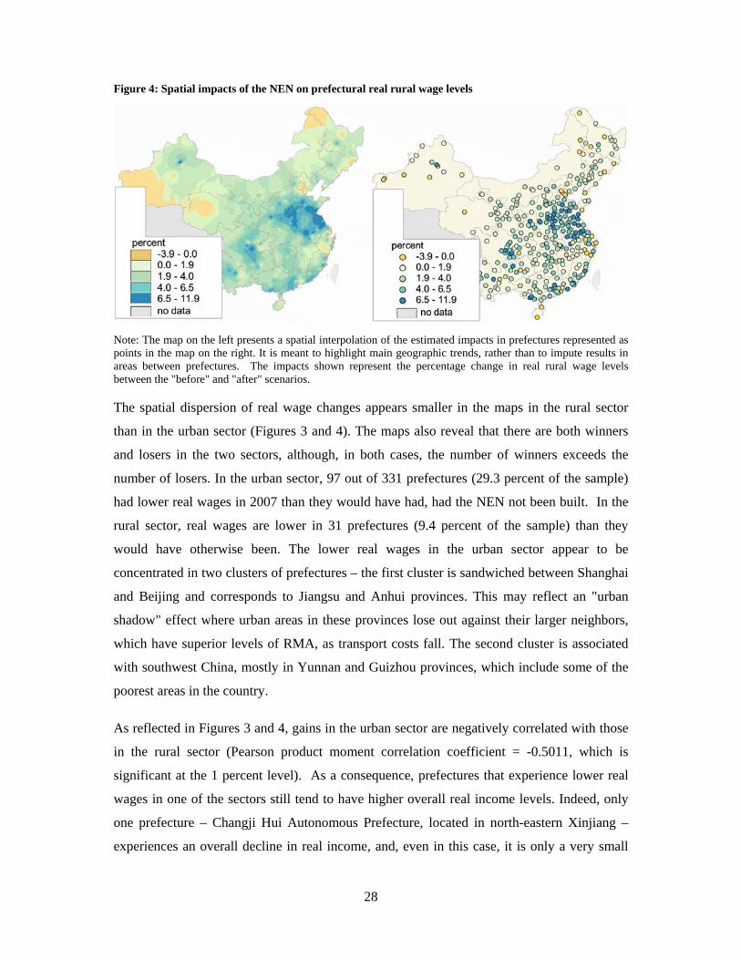
Figure 3: Spatial impacts of the NEN on prefectural real urban wage levels
Note: The map on the left presents a spatial interpolation of the estimated impacts in prefectures represented as points in the map on the right. It is meant to highlight main geographic trends, rather than to impute results in areas between prefectures. The impacts shown represent the percentage change in real urban wage levels between the "before" and "after" scenarios.
27 The respective estimated slope coefficients are 1.300 and -0.647 with associated t-ratios of 1.998 and -2.907. 28 These results may be reconciled by noting that there exists a statistically significant positive correlation between the change in real urban wages experienced by a prefecture and (r = + 0.519; see also the ANOVA exercise in Appendix C). This suggests a tendency for larger real urban wage increases to be concentrated in the prefectures with larger urban sectors, which also tend to be the prefectures with the highest levels of real income per worker (the Pearson product moment correlation coefficient between real income per worker in the "before" scenario and is 0.572).
28
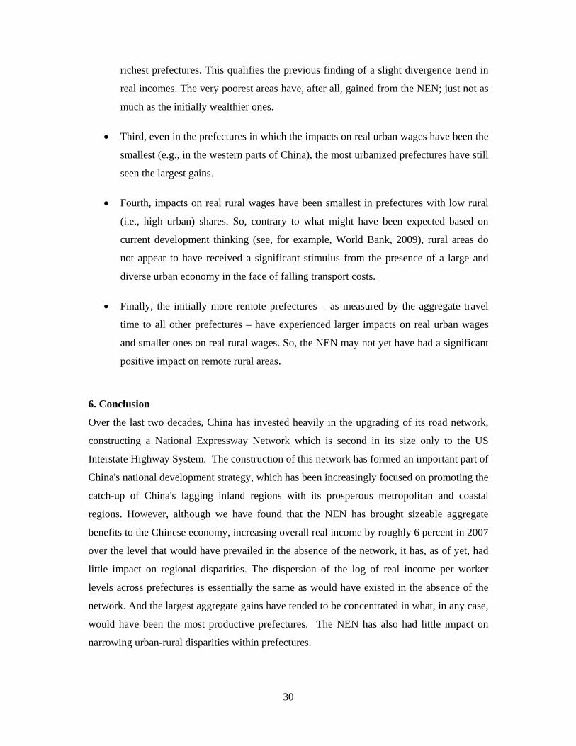
Figure 4: Spatial impacts of the NEN on prefectural real rural wage levels
Note: The map on the left presents a spatial interpolation of the estimated impacts in prefectures represented as points in the map on the right. It is meant to highlight main geographic trends, rather than to impute results in areas between prefectures. The impacts shown represent the percentage change in real rural wage levels between the "before" and "after" scenarios.
The spatial dispersion of real wage changes appears smaller in the maps in the rural sector
than in the urban sector (Figures 3 and 4). The maps also reveal that there are both winners
and losers in the two sectors, although, in both cases, the number of winners exceeds the
number of losers. In the urban sector, 97 out of 331 prefectures (29.3 percent of the sample)
had lower real wages in 2007 than they would have had, had the NEN not been built. In the
rural sector, real wages are lower in 31 prefectures (9.4 percent of the sample) than they
would have otherwise been. The lower real wages in the urban sector appear to be
concentrated in two clusters of prefectures – the first cluster is sandwiched between Shanghai
and Beijing and corresponds to Jiangsu and Anhui provinces. This may reflect an "urban
shadow" effect where urban areas in these provinces lose out against their larger neighbors,
which have superior levels of RMA, as transport costs fall. The second cluster is associated
with southwest China, mostly in Yunnan and Guizhou provinces, which include some of the
poorest areas in the country.
As reflected in Figures 3 and 4, gains in the urban sector are negatively correlated with those
in the rural sector (Pearson product moment correlation coefficient = -0.5011, which is
significant at the 1 percent level). As a consequence, prefectures that experience lower real
wages in one of the sectors still tend to have higher overall real income levels. Indeed, only
one prefecture – Changji Hui Autonomous Prefecture, located in north-eastern Xinjiang –
experiences an overall decline in real income, and, even in this case, it is only a very small

29
one. In particular, Changji Hui's real income falls by 0.53 percent compared to the "before"
scenario.
Although the NEN does not appear to have narrowed regional disparities, we do find that
urban-rural wage ratios within prefectures are very marginally lower than otherwise. In the
"before" scenario, the mean urban-rural wage ratio is 3.01 compared to 2.96 in the "after"
scenario. Also, there is an indication that rural wages have slightly caught-up with urban
wages in those prefectures where they were relatively low, but the evidence from Figure 5 is
that this is a very weak phenomenon.
Figure 5: Impact of the NEN on urban-rural wage ratios within prefectures
0 1 2 3 4 5 6 7 8 90
10
20
30
40
50
60
70
80
90
100Histogram of predicted urban-rural wage ratios
Ratio
Fre
quen
cy
With
Without
0 1 2 3 4 5 6 7 80
1
2
3
4
5
6
7
Predicted urban-rural wage ratio (without)
Pre
dict
ed u
rban
-rur
al w
age
ratio
(w
ith)
Further analysis of variance (ANOVA) of the patterns of estimated changes in real income
and wages reveals a number of insights. We only summarize the main results here, while
Appendix C presents the detailed results.
First, the analysis confirms that as one moves away from the metro and coastal areas,
real urban wage growth diminishes. So in areas that are already fairly urbanized, and
that benefit from the diversity associated with large agglomerations, the NEN appears
to have induced the largest urban wage growth. In contrast, in rural areas, there does
not appear to be a clear trend, although real wages have, on average, fallen in the
three Metro regions – Beijing, Shanghai and Tianjin – and increased by only a
relatively small amount in the north-eastern prefectures.
Second, urban wage growth attributable to the NEN does not seem to be associated
with efficiency adjusted real urban wage levels in the "before" scenario. The largest
impacts on real urban wages have been in the initially poorest and in the initially
30
richest prefectures. This qualifies the previous finding of a slight divergence trend in
real incomes. The very poorest areas have, after all, gained from the NEN; just not as
much as the initially wealthier ones.
Third, even in the prefectures in which the impacts on real urban wages have been the
smallest (e.g., in the western parts of China), the most urbanized prefectures have still
seen the largest gains.
Fourth, impacts on real rural wages have been smallest in prefectures with low rural
(i.e., high urban) shares. So, contrary to what might have been expected based on
current development thinking (see, for example, World Bank, 2009), rural areas do
not appear to have received a significant stimulus from the presence of a large and
diverse urban economy in the face of falling transport costs.
Finally, the initially more remote prefectures – as measured by the aggregate travel
time to all other prefectures – have experienced larger impacts on real urban wages
and smaller ones on real rural wages. So, the NEN may not yet have had a significant
positive impact on remote rural areas.
6. Conclusion
Over the last two decades, China has invested heavily in the upgrading of its road network,
constructing a National Expressway Network which is second in its size only to the US
Interstate Highway System. The construction of this network has formed an important part of
China's national development strategy, which has been increasingly focused on promoting the
catch-up of China's lagging inland regions with its prosperous metropolitan and coastal
regions. However, although we have found that the NEN has brought sizeable aggregate
benefits to the Chinese economy, increasing overall real income by roughly 6 percent in 2007
over the level that would have prevailed in the absence of the network, it has, as of yet, had
little impact on regional disparities. The dispersion of the log of real income per worker
levels across prefectures is essentially the same as would have existed in the absence of the
network. And the largest aggregate gains have tended to be concentrated in what, in any case,
would have been the most productive prefectures. The NEN has also had little impact on
narrowing urban-rural disparities within prefectures.
31
The lack of overall catch-up thus far generated by the NEN is largely attributable to its effect
on the urban sector of the Chinese economy, where the gains across prefectures have, on
average, been larger than in the rural sector. Thus, the impact of the NEN on real urban
wages diminishes as we move inland from the metro and coastal regions. The gradient,
however, is far from smooth – even in the Western parts of China, the more urbanized
prefectures have experienced relatively strong increases in real urban wages. Furthermore,
for almost a third of prefectures, the impact of the NEN on real urban wages has been
negative, so that there have been substantial numbers of losers as well as winners. However,
the prefectures that have lost out in the urban sector have tended to be compensated by
stronger performance in the rural sector. Indeed, more generally, increases in real rural wages
attributable to the NEN have been smaller – negative even – in prefectures located in the
metropolitan and north-eastern regions of China than in other regions.
These findings may run counter to often stated policy preferences for a spatial equalization of
economic growth. But they need to be seen in the context of long-term evidence of
geographic growth patterns within countries (as reviewed in World Bank 2009a).
Concentration of economic activity increases aggregate income and unbalanced economic
growth has been a feature of the development experience in all of today's rich countries. In
the long term, growth is likely to spread out again as firms take advantage of lower transport
costs to escape congestion and higher factor prices. In the short to medium term, public
policies should aim to invest a sufficient share of the gains from agglomeration to ensure
geographically equal access to basic services like education, health, water and electricity.
This will allow citizens to take advantage of economic opportunity locally or after migrating
to a growth area.
The above results are based on an innovative NEG-based methodology in which data
interacts with theory to generate estimated impacts. This methodology, therefore, has the
advantage of combining theoretical coherence and logical rigor with consistency with
available data. As such, it is able to capture the totality of impacts, which work through the
shaping of a country's economic geography, which might otherwise be missed by a more
conventional, purely econometric, impact evaluation approach. However, despite its
advantages, it must be emphasized that the estimates of impact are short-run estimates that do
not take into account possible additional effects associated with the induced migration of
factors of production, particularly labor, that can be expected to occur in response to the

32
reshaping of a country's geography of market potential. It is also possible that falling
transport costs associated with the NEN may have reduced the costs of migration, particularly
of unofficial migration, in China over the time period of its construction. The extension of
our framework to incorporate migration dynamics is an important area of future research
which will be essential to a complete understanding of the eventual full impact of the NEN.
33
Appendix A: Data Appendix
A.1. Economic Data Sources
Data sources The main sources for our prefectural level data are the Regional Economic Statistical Yearbook 2008 and the China Statistical Yearbook 2008, both of which are published by the National Bureau of Statistics of China. We also draw upon the statistical yearbooks of various provinces, most notably, the Chongqing Statistical Yearbook 2008, which are published by the provincial statistics bureaus. Our final dataset consists of 331 prefectural level regions (prefectures for brevity), which account for 86.2 % of China's total land area, 96.2 % of aggregate Chinese population, 93 % of aggregate employment and 99 % of aggregate GDP.29 Unless otherwise stated, all data is for 2007. Prefectural level regions in China Within China, there are four tiers of administrative region. These correspond to: (a) the provincial level, (b) the prefectural level, (c) the county level, and (d) the township level. Restricting our attention to mainland China, the provincial level consists of the 22 provinces, the five autonomous regions (Inner Mongolia, Guangxi, Tibet, Ningxia and Xinjiang), and the four municipalities (Beijing, Chongqing, Tianjin and Shanghai). The municipalities are "cities" under the direct control of central government. Included at the prefectural level are prefectural cities, prefectures, ethnic minority autonomous prefectures, leagues and districts under municipalities. In 2007, there were 333 prefectural level regions30; of which 283 were prefectural cities.31 Given that a prefectural city typically has a significant rural component, the word "city" differs in its meaning from Western usage. A prefectural city more closely resembles a Christaller-style central place system, which comprises a size distribution of settlements. At the county level, a typical prefectural city consists of three types of territorial unit: (i) districts, (ii) counties, and (iii) county-level cities. A prefectural city's districts are contiguous areas which, collectively, represent its "city proper" (Shiqu in Chinese). Although, in many cases, still possessing some agricultural and rural population, they constitute the urban core of a prefectural city. A prefectural city's counties, by contrast, account for the bulk of its rural area. Nevertheless, many counties have their own urban centers. Finally, county-level cities are counties which have been officially renamed as "cities" on account of their urbanization levels. On average, in 2007, 65.4 % of a prefectural city's population was registered as being agricultural. For counties and county-level cities under prefectural cities, the corresponding percentage was around 80 %. 15.5 % of a prefectural city's GDP is, on average, derived from the primary sector, while, for counties and county-level cities under prefectural cities, the percentage is 23.2 %.32
29 All of these figures relate to mainland China. 30 The 4 municipalities and their sub-regions are not counted. 31 Among these 283 prefectural cities, there are 15 sub-provincial cities, which have greater independence in the administration of economy and law than other ordinary prefectural cities. These cities are: Wuhan, Chengdu, Xi’an, Harbin, Changchun, Shenyang, Dalian, Jina, Qingdao, Nanjing, Hangzhou, Ningbo, Xiamen, Guangzhou and Shenzhen. 32 13 prefectural cities do not have any counties or county-level cities. The averages reported therefore exclude these cities.
34
Prefectures, ethnic minority autonomous prefectures and leagues are all less urbanized than prefectural cities. Ethnic minority autonomous prefectures and leagues are also dominated by ethnic minority populations. Districts under municipalities are at the prefectural level administratively, even though districts under prefectural cities are at the county level. To maximise sample size and geographic coverage, our dataset includes 280 of China's 283 prefectural cities, 11 of its 17 prefectures, all 30 of its ethnic minority autonomous prefectures, and all three of its leagues. The three prefectural cities which are excluded are Tianshui City (Gansu Province), Karamay City (Xinjiang), Lhasa City (Tibet). Meanwhile, the excluded prefectures are Ngari, Nagqu, Qamdo, Xigazê, Shannan and Nyingchi (all Tibet). With the exception of Karamay City, which is located in China's remote western region and whose economic structure is heavily biased by dominance of the oil production and refining industry, all of these exclusions are attributable to a lack of data availability. Also included as "prefectures" in our dataset are three of the four municipalities – Beijing, Shanghai and Tianjin – which operate at the provincial level, whilst we divide the fourth municipality – Chongqing – into three regions ("One-Hour Economic Circle", "Northeast wing" and "Southeast wing"). In terms of population and land area, Beijing, Shanghai and Tianjin more closely resemble the larger prefectural cities than they do the 22 provinces. Chongqing Municipality looks more like a small province, hence our division of it into three regions. These three regions correspond to those identified in Chongqing Municipal Government's Master Plan for Experimental Reform (World Bank, 2009).33 Shihezi City, a county-level city under the direct jurisdiction of Xinjiang Province, also enters our dataset.34 Our sample size of 331 regions exceeds that of previous studies in the empirical NEG literature which have made use of prefectural level data (Au and Henderson, 2006; Hering and Poncet, 2010a; and Bosker et al., 2010). This is because these studies have, by and large, restricted themselves to prefectural level cities. Variables used in the estimation of the urban and rural wage equations Urban wage rate (wU): proxied by average disposable income per capita for urban households. Urban household disposable income is the actual income at the disposal of members of a household which can be used for final consumption, other non-compulsory expenditure and savings. It is equal to the total income of an urban household minus payments to cover income tax and personal contributions to social security, and the income subsidy received by a sample household for keeping a diary. Source: Regional Economic Statistical Yearbook 2008.
Data is missing for 14 prefectures on this variable. These missing values have been filled-in using the predicted values generated from OLS estimation of the regression equation:
33 Prior to 1997, Chongqing was a sub-provincial city in Sichuan province. The area that was added to Chongqing as part of its upgrading to a municipality in 1997 mainly consists of the two wings, i.e. the Northeast and Southeast wings. 34 There are 4 county-level cities in Xinjiang that are under the direct jurisdiction of Xinjiang Province. These cities are also called "sub-prefecture-level cities" or "vice-prefecture-level cities" (http://en.wikipedia.org/wiki/ Sub-prefecture-level_city). Shihezi City is included in our sample because, after Urumqi, it is the second largest city in terms of population in Xinjiang (http://en.wikipedia.org/wiki/Shihezi). It is also the only sub-prefecture-level city in Xinjiang for which adequate data was available.

35
iiiiiiiiUU
i LATLONGLATLONGLATLONGPWGDPcw )()()(_ 22 [A1]
for the 317 non-missing observations, where GDP_PWi denotes the GDP per worker of prefecture i, LONGi its longitude and LATi its latitude. The longitude and latitude for a prefecture both refer to its geographic center. The estimated regression has R2 = 0.70. Rural wage rate (wR): proxied by average net income per capita for rural households. The net income of a rural household is its total income from all sources minus all corresponding expenses. Expenses in this context consist of household operation expenses, taxes and fees, an allowance for depreciation of fixed assets used in rural production, and gifts made to non-rural residents. The income subsidy received for survey participation is also subtracted. Source: Regional Economic Statistical Yearbook 2008. Data is missing for one prefecture on this variable. The value of the missing observation has been filled-in using the predicted value generated from OLS estimation of an equation analogous to equation [A1] for wR for the 330 non-missing observations (R2 = 0.73). Income (Y): in constructing the measures of real market access for the urban and rural sectors (RMAU and RMAR respectively), a measure of income is required. The measure used is GDP. Data source: Regional Economic Statistical Yearbook 2008, Investment per worker (I pw): measured separately for the urban and rural sectors as fixed investment per worker. Data source: Regional Economic Statistical Yearbook 2008. Human capital (human): for both the urban and rural sectors, proxied by the average number of years of education held by a prefecture's population in 2000. Data source: China 2000 Population Census Data Assembly. The spatial lags of ln(I pw) and ln(human), i.e. W*ln(I pw) and W*ln(human), which also enter into the estimation of the urban and rural wage equations as control variables, are constructed through pre-multiplying the column vectors of observations on ln(I pw) and ln(human) by the spatial weights matrix, W. The i-jth element of this matrix, wij, equals 1 if regions i and j share a contiguity relationship; otherwise, wij = 0. Contiguity is inferred from the geographic co-ordinates of the centers of the prefectures using a Delaunay trianglarization scheme. To implement this scheme, we use the xy2cont MatLab function from James LeSage's spatial econometrics toolbox (downloadable from www.spatial-econometrics.com). The W matrix is row-standardized so that the elements on the ith row sum to unity. Instrumental variables In estimating the urban and rural wage equations, equations [10] and [11], using 2SLS and the FGS2SLS estimator, the following instruments are used for, the (natural) logarithms of, domestic urban and rural real market access: Urban:
jijj darea )]}]1(/[1{ln[ , W*W* ln(I pw)
Rural: W*W*ln(I pw), W*W*ln(human), )1ln( 45.0iportd
36
where dij is the Euclidean distance between the geographic centers of prefectures i and j, diport
is the Euclidean distance between the center of region i and that of the nearest prefecture which has a major international port, and area is a prefecture's land area (in km2). The data on land areas is taken from Regional Economic Statistical Yearbook 2008. Eight major international ports are considered: Shanghai, Ningbo, Tianjin, Guangzhou, Qingdao City, Dalian City, Qinhuangdao City and Shenzhen City. These correspond to the eight Chinese ports which had the largest throughput (measured in million tonnes of traffic) in ISL (2006). Pre-multiplication of a variable by W*W represents the second-order spatial lag of that variable. Additional parameters used in the numerical solution of the theoretical model: As outlined in section 3.2, to obtain a numerical solution for the system of equations [3] – [7], which describe the short-run equilibrium of our theoretical model, we also require measures for the parameters , , . For 2007, the measures for and , which correspond to the regional shares of the national urban and rural workforces respectively, are constructed using data on "urban employed persons" and "total employed persons" from the Regional Economic Statistical Yearbook 2008. For , rural employment is calculated as total employed persons minus urban employed persons 35 According to the China Statistical Yearbook 2008, employed persons refer to "people aged 16 and over who are engaged in gainful employment and thus receive remuneration payment or earn business income". , the national share of urban workers in total employment, is measured using the same data. The data on "total employed persons" is also used in the calculation of GDP per worker for 2007, which is used to help assess the fit of the "after" equilibrium solution. GDP per capita for 2007, which is also used in assessing the fit, is measured using population data from Regional Economic Statistical Yearbook 2008. Table A1 provides summary statistics for both the variables used in the estimation of the wage equations and the additional parameters used in obtaining the "before" and "after" numerical solutions to our model.
35 In the various provincial statistical yearbooks, the numbers of urban and rural employed persons exactly sum to the number of total employed persons at the provincial level.
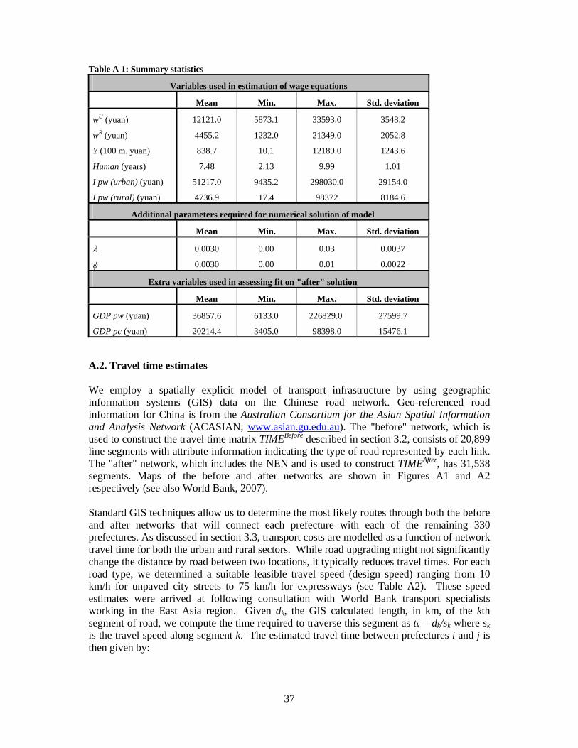
37
Table A 1: Summary statistics
Variables used in estimation of wage equations
Mean Min. Max. Std. deviation
wU (yuan)
wR (yuan)
Y (100 m. yuan)
Human (years)
I pw (urban) (yuan)
I pw (rural) (yuan)
12121.0
4455.2
838.7
7.48
51217.0
4736.9
5873.1
1232.0
10.1
2.13
9435.2
17.4
33593.0
21349.0
12189.0
9.99
298030.0
98372
3548.2
2052.8
1243.6
1.01
29154.0
8184.6
Additional parameters required for numerical solution of model
Mean Min. Max. Std. deviation
0.0030
0.0030
0.00
0.00
0.03
0.01
0.0037
0.0022
Extra variables used in assessing fit on "after" solution
Mean Min. Max. Std. deviation
GDP pw (yuan)
GDP pc (yuan)
36857.6
20214.4
6133.0
3405.0
226829.0
98398.0
27599.7
15476.1
A.2. Travel time estimates We employ a spatially explicit model of transport infrastructure by using geographic information systems (GIS) data on the Chinese road network. Geo-referenced road information for China is from the Australian Consortium for the Asian Spatial Information and Analysis Network (ACASIAN; www.asian.gu.edu.au). The "before" network, which is used to construct the travel time matrix TIMEBefore described in section 3.2, consists of 20,899 line segments with attribute information indicating the type of road represented by each link. The "after" network, which includes the NEN and is used to construct TIMEAfter, has 31,538 segments. Maps of the before and after networks are shown in Figures A1 and A2 respectively (see also World Bank, 2007). Standard GIS techniques allow us to determine the most likely routes through both the before and after networks that will connect each prefecture with each of the remaining 330 prefectures. As discussed in section 3.3, transport costs are modelled as a function of network travel time for both the urban and rural sectors. While road upgrading might not significantly change the distance by road between two locations, it typically reduces travel times. For each road type, we determined a suitable feasible travel speed (design speed) ranging from 10 km/h for unpaved city streets to 75 km/h for expressways (see Table A2). These speed estimates were arrived at following consultation with World Bank transport specialists working in the East Asia region. Given dk, the GIS calculated length, in km, of the kth segment of road, we compute the time required to traverse this segment as tk = dk/sk where sk is the travel speed along segment k. The estimated travel time between prefectures i and j is then given by:
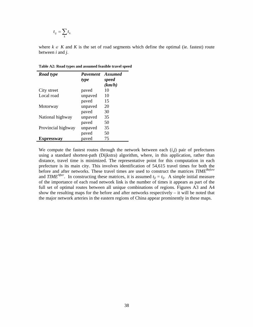
38
k
kij tt
where k K and K is the set of road segments which define the optimal (ie. fastest) route between i and j.
Table A2: Road types and assumed feasible travel speed
Road type Pavement type
Assumed speed (km/h)
City street paved 10 Local road unpaved 10 paved 15 Motorway unpaved 20 paved 30 National highway unpaved 35 paved 50 Provincial highway unpaved 35 paved 50 Expressway paved 75 We compute the fastest routes through the network between each (i,j) pair of prefectures using a standard shortest-path (Dijkstra) algorithm, where, in this application, rather than distance, travel time is minimized. The representative point for this computation in each prefecture is its main city. This involves identification of 54,615 travel times for both the before and after networks. These travel times are used to construct the matrices TIMEBefore and TIMEAfter. In constructing these matrices, it is assumed tji = tij. A simple initial measure of the importance of each road network link is the number of times it appears as part of the full set of optimal routes between all unique combinations of regions. Figures A3 and A4 show the resulting maps for the before and after networks respectively – it will be noted that the major network arteries in the eastern regions of China appear prominently in these maps.
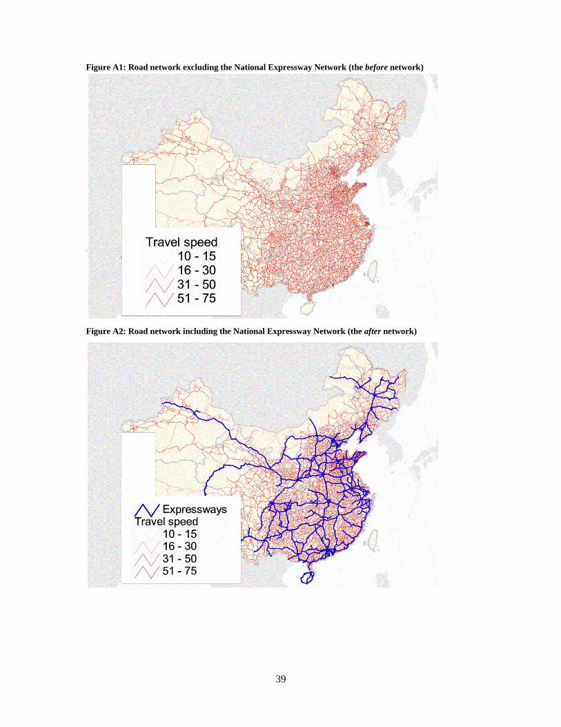
39
Figure A1: Road network excluding the National Expressway Network (the before network)
Figure A2: Road network including the National Expressway Network (the after network)
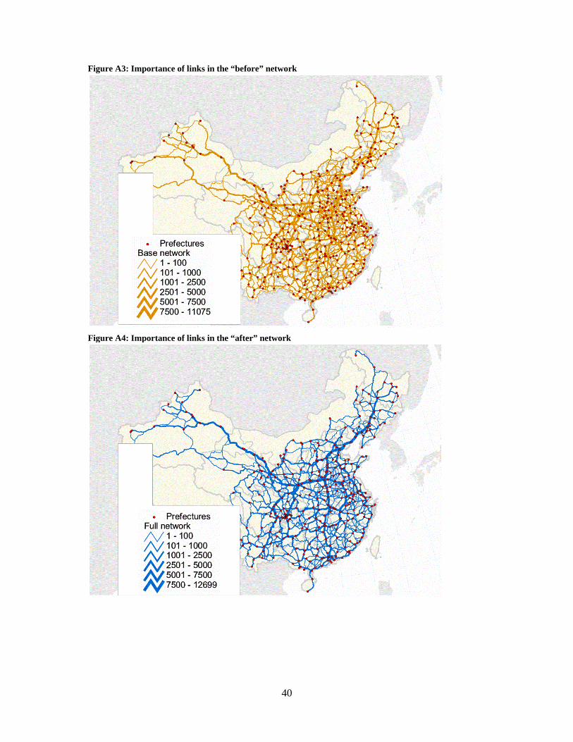
40
Figure A3: Importance of links in the “before” network
Figure A4: Importance of links in the “after” network
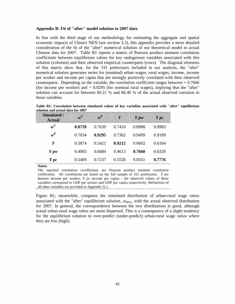
41
Appendix B: Fit of "after" model solution to 2007 data In line with the third stage of our methodology for estimating the aggregate and spatial economic impacts of China's NEN (see section 3.2), this appendix provides a more detailed consideration of the fit of the "after" numerical solution of our theoretical model to actual Chinese data for 2007. Table B1 reports a matrix of Pearson product moment correlation coefficients between equilibrium values for key endogenous variables associated with this solution (columns) and their observed empirical counterparts (rows). The diagonal elements of this matrix show that, for the 331 prefectures included in our analysis, the "after" numerical solution generates series for (nominal) urban wages, rural wages, income, income per worker and income per capita that are strongly positively correlated with their observed counterparts. Depending on the variable, the correlation coefficient ranges between + 0.7660 (for income per worker) and + 0.9295 (for nominal rural wages), implying that the "after" solution can account for between 60.21 % and 86.40 % of the actual observed variation in these variables. Table B1: Correlation between simulated values of key variables associated with "after" equilibrium solution and actual data for 2007
Simulated / Actual
wU wR Y Y pw Y pc
wU 0.8739 0.7639 0.7410 0.8988 0.8983
wR 0.7034 0.9295 0.7362 0.9499 0.9189
Y 0.5874 0.5421 0.9212 0.6602 0.6164
Y pw 0.4083 0.6684 0.4613 0.7660 0.6320
Y pc 0.5409 0.7237 0.5558 0.8351 0.7776
Notes: The reported correlation co-efficients are Pearson product moment correlation coefficients. All correlations are based on the full sample of 331 prefectures. Y pw denotes income per worker; Y pc income per capita - the observed values of these variables correspond to GDP per worker and GDP per capita respectively. Definitions of all other variables are provided in Appendix A.1. Figure B1, meanwhile, compares the simulated distribution of urban-rural wage ratios associated with the "after" equilibrium solution, After, with the actual observed distribution for 2007. In general, the correspondence between the two distributions is good, although actual urban-rural wage ratios are more dispersed. This is a consequence of a slight tendency for the equilibrium solution to over-predict (under-predict) urban-rural wage ratios where they are low (high).
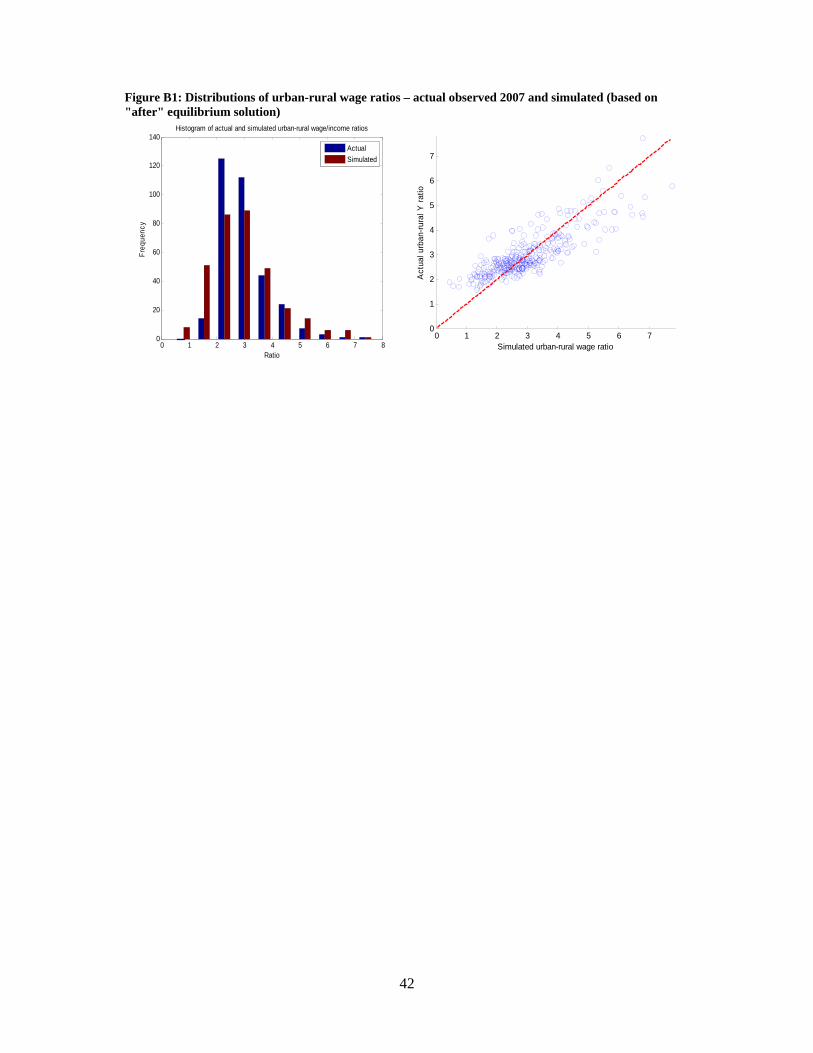
42
0 1 2 3 4 5 6 7 80
20
40
60
80
100
120
140Histogram of actual and simulated urban-rural wage/income ratios
Ratio
Fre
quen
cy
Actual
Simulated
Figure B1: Distributions of urban-rural wage ratios – actual observed 2007 and simulated (based on "after" equilibrium solution)
0 1 2 3 4 5 6 70
1
2
3
4
5
6
7
Simulated urban-rural wage ratio
Act
ual u
rban
-rur
al Y
rat
io
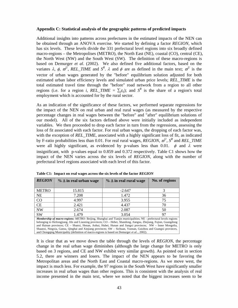
43
Appendix C: Statistical analysis of the geographic patterns of predicted impacts
Additional insights into patterns across prefectures in the estimated impacts of the NEN can be obtained through an ANOVA exercise. We started by defining a factor REGION, which has six levels. These levels divide the 331 prefectural level regions into six broadly defined macro-regions – the Metropolises (METRO), the North East (NE), coastal (CO), central (CE), the North West (NW) and the South West (SW). The definition of these macro-regions is based on Demurger et al. (2002). We also defined five additional factors, based on the variates , , U, REL_TIME and SR. and are as defined in the main text; U is the vector of urban wages generated by the "before" equilibrium solution adjusted for both estimated urban labor efficiency levels and simulated urban price levels; REL_TIME is the total estimated travel time through the "before" road network from a region to all other regions (i.e. for a region i, REL_TIME = jtij); and SR is the share of a region's total employment which is accounted for by the rural sector.
As an indication of the significance of these factors, we performed separate regressions for the impact of the NEN on real urban and real rural wages (as measured by the respective percentage changes in real wages between the "before" and "after" equilibrium solutions of our model). All of the six factors defined above were initially included as independent variables. We then proceeded to drop each factor in turn from the regressions, assessing the loss of fit associated with each factor. For real urban wages, the dropping of each factor was, with the exception of REL_TIME, associated with a highly significant loss of fit, as indicated by F-ratio probabilities less than 0.01. For real rural wages, REGION, U, SR and REL_TIME were all highly significant, as evidenced by p-values less than 0.01. and were insignificant, with p-values equal to 0.859 and 0.372 respectively. Table C1 shows how the impact of the NEN varies across the six levels of REGION, along with the number of prefectural level regions associated with each level of this factor.
Table C1: Impact on real wages across the six levels of the factor REGION
REGION % in real urban wage % in real rural wage
No. of regions
METRO 15.815 -2.647 3NE 7.208 1.472 36CO 4.997 3.955 75CE 2.421 4.437 70NW 2.674 2.087 50SW 1.479 3.054 97Membership of macro-regions: METRO- Beijing, Shanghai and Tianjin municipalities; NE - prefectural levels regions belonging to Heilongjiang, Jiln and Liaoning provinces; CO – Hebei, Shandong, Jiangsu, Zhejiang, Fujian, Guangdong and Hainan provinces; CE – Shanxi, Henan, Anhui, Hubei, Hunan and Jiangxi provinces; NW – Inner Mongolia, Shaanxi, Ningxia, Gansu, Qinghai and Xinjiang provinces; SW – Sichuan, Yunnan, Guizhou and Guangxi provinces, and Chongqing Municipality (definition of macro-regions is based on Demurger et al.., 2002).
It is clear that as we move down the table through the levels of REGION, the percentage change in the real urban wage diminishes (although the large change for METRO is only based on 3 regions, and CE and NW exhibit very similar growth). As pointed out in section 5.2, there are winners and losers. The impact of the NEN appears to be favoring the Metropolitan areas and the North East and Coastal macro-regions. As we move west, the impact is much less. For example, the 97 regions in the South West have significantly smaller increases in real urban wages than other regions. This is consistent with the analysis of real income presented in the main text, where we noted that the biggest increases seem to be
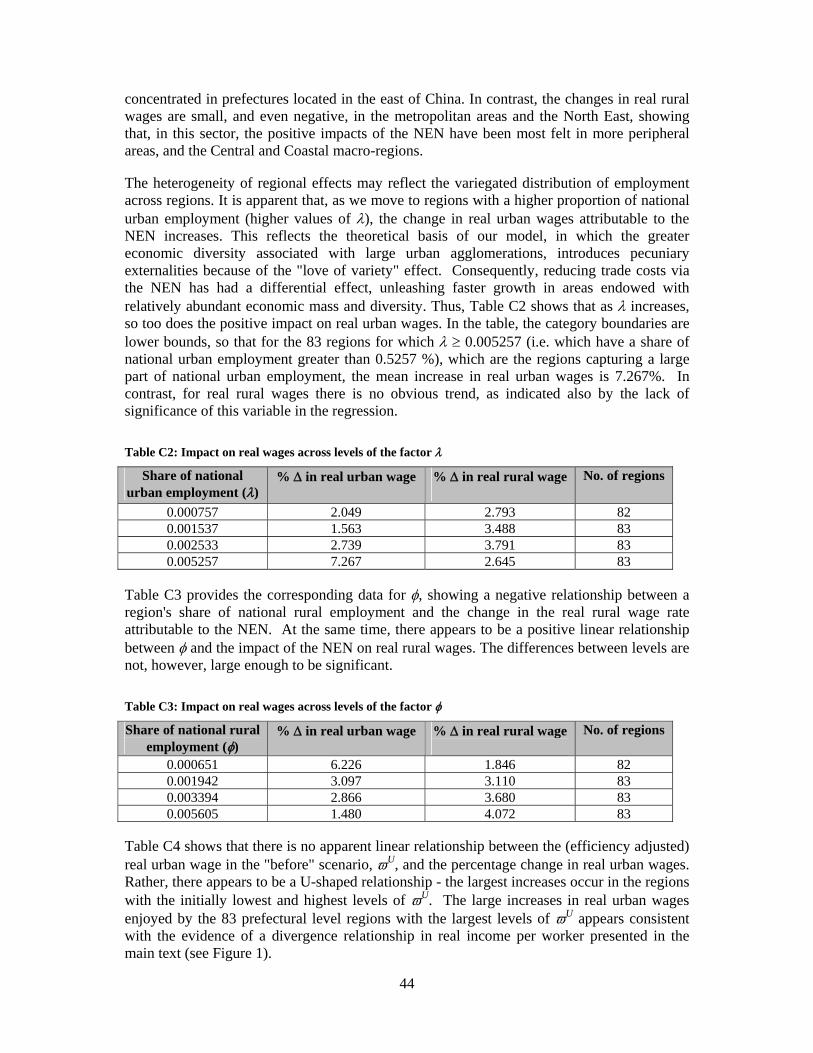
44
concentrated in prefectures located in the east of China. In contrast, the changes in real rural wages are small, and even negative, in the metropolitan areas and the North East, showing that, in this sector, the positive impacts of the NEN have been most felt in more peripheral areas, and the Central and Coastal macro-regions.
The heterogeneity of regional effects may reflect the variegated distribution of employment across regions. It is apparent that, as we move to regions with a higher proportion of national urban employment (higher values of ), the change in real urban wages attributable to the NEN increases. This reflects the theoretical basis of our model, in which the greater economic diversity associated with large urban agglomerations, introduces pecuniary externalities because of the "love of variety" effect. Consequently, reducing trade costs via the NEN has had a differential effect, unleashing faster growth in areas endowed with relatively abundant economic mass and diversity. Thus, Table C2 shows that as increases, so too does the positive impact on real urban wages. In the table, the category boundaries are lower bounds, so that for the 83 regions for which 0.005257 (i.e. which have a share of national urban employment greater than 0.5257 %), which are the regions capturing a large part of national urban employment, the mean increase in real urban wages is 7.267%. In contrast, for real rural wages there is no obvious trend, as indicated also by the lack of significance of this variable in the regression.
Table C2: Impact on real wages across levels of the factor
Share of national urban employment ()
% in real urban wage % in real rural wage
No. of regions
0.000757 2.049 2.793 82 0.001537 1.563 3.488 83 0.002533 2.739 3.791 83 0.005257 7.267 2.645 83
Table C3 provides the corresponding data for , showing a negative relationship between a region's share of national rural employment and the change in the real rural wage rate attributable to the NEN. At the same time, there appears to be a positive linear relationship between and the impact of the NEN on real rural wages. The differences between levels are not, however, large enough to be significant.
Table C3: Impact on real wages across levels of the factor
Share of national rural employment ()
% in real urban wage % in real rural wage
No. of regions
0.000651 6.226 1.846 82 0.001942 3.097 3.110 83 0.003394 2.866 3.680 83 0.005605 1.480 4.072 83
Table C4 shows that there is no apparent linear relationship between the (efficiency adjusted) real urban wage in the "before" scenario, U, and the percentage change in real urban wages. Rather, there appears to be a U-shaped relationship - the largest increases occur in the regions with the initially lowest and highest levels of U. The large increases in real urban wages enjoyed by the 83 prefectural level regions with the largest levels of U appears consistent with the evidence of a divergence relationship in real income per worker presented in the main text (see Figure 1).
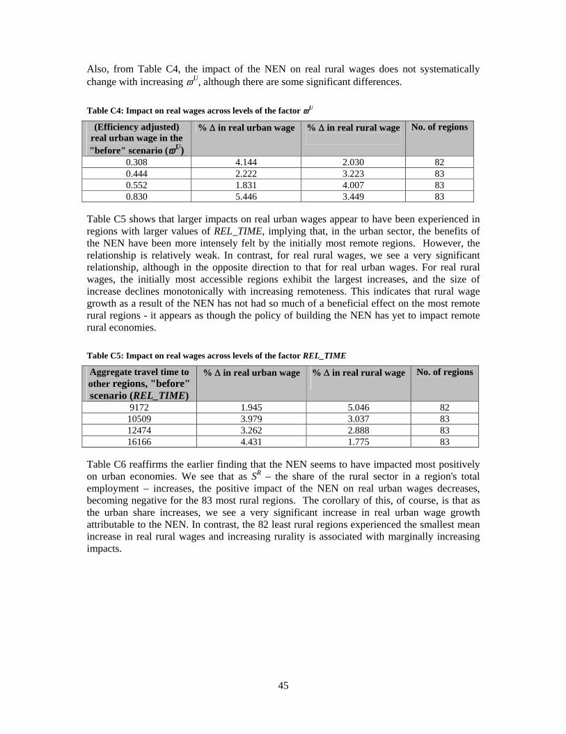
45
Also, from Table C4, the impact of the NEN on real rural wages does not systematically change with increasing U, although there are some significant differences.
Table C4: Impact on real wages across levels of the factor U
(Efficiency adjusted) real urban wage in the "before" scenario (U)
% in real urban wage % in real rural wage
No. of regions
0.308 4.144 2.030 82 0.444 2.222 3.223 83 0.552 1.831 4.007 83 0.830 5.446 3.449 83
Table C5 shows that larger impacts on real urban wages appear to have been experienced in regions with larger values of REL_TIME, implying that, in the urban sector, the benefits of the NEN have been more intensely felt by the initially most remote regions. However, the relationship is relatively weak. In contrast, for real rural wages, we see a very significant relationship, although in the opposite direction to that for real urban wages. For real rural wages, the initially most accessible regions exhibit the largest increases, and the size of increase declines monotonically with increasing remoteness. This indicates that rural wage growth as a result of the NEN has not had so much of a beneficial effect on the most remote rural regions - it appears as though the policy of building the NEN has yet to impact remote rural economies.
Table C5: Impact on real wages across levels of the factor REL_TIME
Aggregate travel time to other regions, "before" scenario (REL_TIME)
% in real urban wage % in real rural wage
No. of regions
9172 1.945 5.046 82 10509 3.979 3.037 83 12474 3.262 2.888 83 16166 4.431 1.775 83
Table C6 reaffirms the earlier finding that the NEN seems to have impacted most positively on urban economies. We see that as SR – the share of the rural sector in a region's total employment – increases, the positive impact of the NEN on real urban wages decreases, becoming negative for the 83 most rural regions. The corollary of this, of course, is that as the urban share increases, we see a very significant increase in real urban wage growth attributable to the NEN. In contrast, the 82 least rural regions experienced the smallest mean increase in real rural wages and increasing rurality is associated with marginally increasing impacts.

46
Table C6: Impact on real wages across levels of the factor SR
Rural sector share of total employment (SR)
% in real urban wage % in real rural wage
No. of regions
0.472 9.819 0.923 82 0.676 4.080 3.401 83 0.786 1.028 4.007 83 0.858 -1.216 4.365 83
To explore interaction effects between the levels of REGION and the levels of the other factors, we fit additional regressions for the impacts on real urban and real rural wages which include interaction terms. Hence, as well as the main effects for each factor considered above, the model includes the interaction terms REGION*, REGION*, REGION*U, REGION*REL_TIME and REGION*SR. Dropping each interaction term from the full model indicates that REGION* (for real urban wages) and REGION*SR (for real rural wages) are the only two significant interactions, with p-values of 0.004 and < 0.001 respectively.
Table C7 and C8 show the impacts of the NEN on real urban wages for the REGION* interaction. The lack of orthogonality between the two factors is apparent from the empty cells. For instance, the three METRO prefectural level regions are obviously in the highest category in terms of share of national urban employment. The table clearly identifies the fact that while the impact on real urban wages diminishes as we move inland, away from the METRO, north-eastern and coastal regions, there are some exceptions. In particular, consistent with previous results, a prefectural level region which is characterized by a large urban-oriented economy experiences major benefits from the NEN - this is reflected by the large estimated impacts on real urban wages for prefectures in the highest category of , more or less regardless of the level of REGION. Hence, even in the South West, which, in general, experiences little positive impact from the NEN, the 15 prefectural level regions at the highest level of urban share enjoy much larger positive impacts on real urban wages than other South West regions.
Table C7: Impact on real urban wages by macro-region (REGION) and share of national urban employment ()
Share of national urban employment ()
0.000757 0.001537 0.002533 0.005257
REGION Macro-region METRO Metropolitan areas * * * 15.815
NE North East 8.537 4.433 7.817 11.040 CO Coastal 6.276 0.281 2.403 7.356 CE Central 5.178 3.108 0.977 2.530 NW North West 1.950 1.112 4.395 15.262 SW South West 0.145 -0.226 1.900 7.549
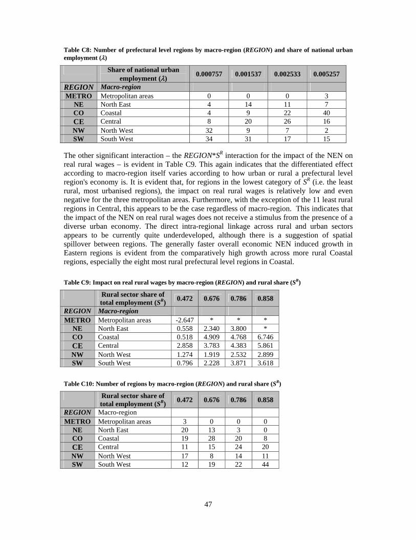
47
Table C8: Number of prefectural level regions by macro-region (REGION) and share of national urban employment ()
Share of national urban employment ()
0.000757 0.001537 0.002533 0.005257
REGION Macro-region METRO Metropolitan areas 0 0 0 3
NE North East 4 14 11 7 CO Coastal 4 9 22 40 CE Central 8 20 26 16 NW North West 32 9 7 2 SW South West 34 31 17 15
The other significant interaction – the REGION*SR interaction for the impact of the NEN on real rural wages – is evident in Table C9. This again indicates that the differentiated effect according to macro-region itself varies according to how urban or rural a prefectural level region's economy is. It is evident that, for regions in the lowest category of SR (i.e. the least rural, most urbanised regions), the impact on real rural wages is relatively low and even negative for the three metropolitan areas. Furthermore, with the exception of the 11 least rural regions in Central, this appears to be the case regardless of macro-region. This indicates that the impact of the NEN on real rural wages does not receive a stimulus from the presence of a diverse urban economy. The direct intra-regional linkage across rural and urban sectors appears to be currently quite underdeveloped, although there is a suggestion of spatial spillover between regions. The generally faster overall economic NEN induced growth in Eastern regions is evident from the comparatively high growth across more rural Coastal regions, especially the eight most rural prefectural level regions in Coastal.
Table C9: Impact on real rural wages by macro-region (REGION) and rural share (SR)
Rural sector share of total employment (SR) 0.472 0.676 0.786 0.858
REGION Macro-region METRO Metropolitan areas -2.647 * * *
NE North East 0.558 2.340 3.800 *CO Coastal 0.518 4.909 4.768 6.746CE Central 2.858 3.783 4.383 5.861NW North West 1.274 1.919 2.532 2.899SW South West 0.796 2.228 3.871 3.618
Table C10: Number of regions by macro-region (REGION) and rural share (SR)
Rural sector share of total employment (SR) 0.472 0.676 0.786 0.858
REGION Macro-region METRO Metropolitan areas 3 0 0 0
NE North East 20 13 3 0CO Coastal 19 28 20 8CE Central 11 15 24 20NW North West 17 8 14 11SW South West 12 19 22 44

48
References Anselin, Luc and Harry H. Kelejian, 1997, "Testing for spatial error autocorrelation in the
presence of endogenous regressors", International Regional Science Review, 20(1-2), 153-182.
Aschauer, David A., 1989, "Is Public Expenditure Productive?", Journal of Monetary Economics, 23(2), 177-200.
Au, Chun-Chung and J.Vernon Henderson, 2006, "Are Chinese Cities too Small?", Review of Economic Studies, 73(3), 549-576.
Bosker, Maarten, Steven Brakman, Harry Garretsen and Marc Schramm, 2010, " The New Economic Geography of Prefecture Cities in China: The Relevance of Market Access and Labor Mobility for Agglomeration", mimeo.
Brakman, Steven, Harry Garretsen and Marc Schramm, 2006, "Putting New Economic Geography to the Test", Regional Science and Urban Economics, 36(5), 613-635.
Brakman, Steven, Harry Garretsen and Charles van Marrewijk, 2009, The New Introduction to Geographical Economics, 2nd edition, Cambridge: Cambridge University Press.
Bröcker, Johannes (2002), "Spatial Effects of European Transport Policy: a CGE Approach", in Geoffery J.D. Hewings, M. Sonis and D. Boyce (eds.), Trade, Network and Hierarchies: Modeling Regional and Interegional Economies, Advances in Spatial Science, Berlin: Springer.
Chandra, Amitabh and Eric Thompson, 2000, "Does Public Infrastructure Affect Economic Activity? Evidence From The Rural Interstate Highway System", Regional Science and Urban Economics, 30(4), 457-490.
Combes, Pierre-Philippe and Miren Lafourcade, 2005, "Transport costs: measures, determinants, and regional policy implications for France", Journal of Economic Geography, 5(3), 319-349.
Démurger, Sylvie, Jeffrey D. Sachs, Wing Thye Woo, Shuming Bao, Gene Chang and Andrew Mellinger, 2002, "Geography, Economic Policy, and Regional Development in China", Asian Economic Papers, 1(1), 146-197.
Emran, M. Shahe and Zhaoyang Hou, 2008, "Access to Markets and Household Consumption: Evidence from Rural China", Department of Economics, George Washington University, mimeo.
Fernald, John G., 1999, "Roads to Prosperity? Assessing the Link between Public Capital and Productivity", American Economic Review, 89(3), 619-638.
Fingleton, Bernard, 2005a, "Beyond neoclassical orthodoxy: A view based on the new economic geography and UK regional wage data", Papers in Regional Science, 84(3), 351-375.
Fingleton, Bernard, 2005b, "Towards Applied Geographical Economics: Modelling Relative Wage Rates, Incomes and Prices for the Regions of Great Britain", Applied Economics, 37(21), 2417-2428.
Fingleton, Bernard, 2006, "The New Economic Geography Versus Urban Economics: an Evaluation Using Local Wage Rates in Great Britain", Oxford Economic Papers, 58(3), 501-530.
49
Fingleton, Bernard, 2007, "New Economic Geography: Some Preliminaries", in Bernard Fingleton (ed.), New Directions in Economic Geography, Cheltenham: Edward Elgar.
Fingleton, Bernard, 2008, "Competing Models of Global Dynamics: Evidence from Panel Models with Spatially Correlated Error Components", Economic Modelling, 25(3), 542-558.
Fingleton, Bernard and Manfred M. Fischer, 2009, "Neoclassical Theory versus New Economic Geography: Competing Explanations of Cross-Regional Variation in Economic Development", Annals of Regional Science, 44(3), 467-491.
Fingleton, Bernard and Julie LeGallo, 2008, "Estimating Spatial Models with Endogenous Variables, a Spatial Lag and Spatially Dependent Distrurbances: Finite Sample Properties", Papers in Regional Science, 87(3), 319-339.
Fingleton, Bernard and Philip McCann, 2007, "Sinking the Iceberg? On the Treatment of Transport Costs in New Economic Geography", in Bernard Fingleton (ed.), New Directions in Economic Geography, Cheltenham: Edward Elgar.
Fujita, Masahisa, Anthony J. Venables and Paul R. Krugman, 1999, The Spatial Economy: Cities, Regions and International Trade, Cambridge. Mass: MIT Press.
Hanson, Gordon H., 1997, "Increasing Returns, Trade and the Regional Structure of Wages", Economic Journal, 107(440), 113-33.
Hanson, Gordon H., 2005, "Market Potential, Increasing Returns and Geographic Concentration", Journal of International Economics, 67(1), 1-24.
Hering, Laura and Sandra Poncet, 2010a, "Income per Capita Inequality in China: the Role of Economic Geography and Spatial Interactions", The World Economy, 33(5), 655-797.
Hering, Laura and Sandra Poncet (2010b), "Market Access and Individual Wages: Evidence from China", Review of Economics and Statistics, 92(1), 145-59.
Hong, Junjie, Anthony T.H. Chin and Binglian Liu, 2004, "Logistics Outsourcing by Manufacturers in China: A Survey of the Industry," Transportation Journal, 43(1), 17-25.
ISL, 2006, "Shipping Statistical Yearbook 2006", Bremen: Institute of Shipping Economics and Logistics.
Keeler, Theodore E. and John S. Ying (1988), "Measuring the Benefits of Large Public Investment. The Case of the U.S. Federal-Aid Highway System", Journal of Public Economics, 36(1), 69-85.
Kelejian, Harry H. and Ingmar R. Prucha, 1998, "A Generalized Spatial Two Stage Least Squares Procedure for Estimating a Spatial Autoregressive Model with Autoregressive Disturbances", with H.H. Kelejian, Journal of Real Estate Finance and Economics, 17(1), 99-121.
Krugman, Paul R., 1991a, Geography and Trade, Cambridge, Mass.: MIT Press.
Krugman, Paul R., 1991b, "Increasing Returns and Economic Geography", Journal of Political Economy, 99(?), 483-499.
Laird, James J., John Nellthorp and Peter J. Mackie, 2005, "Network Effects and Total Economic Impact in Transport Appraisal", Transport Policy, 12(?), 537-544.
McCann, Philip, 2005, "Transport Costs and New Economic Geography", Journal of Economic Geography, 5(3), 305-318.
50
Meng, Xin, Robert Gregory and Youjuan Wang, 2005, "Poverty, Inequality and Growth in Urban China, 1986–2000", Journal of Comparative Economics, 33(4), 710–29.
Martin, Ronald L., 1999, "The New 'Geographical Turn' in Economics: Some Critical Reflections", Cambridge Journal of Economics, 23(1), 63-91.
Mayer, Thierry, 2008, "Market Potential and Development", Centre for Economic Policy Research Discussion Paper No. 6798.
Michaels, Guy, 2008, "The Effect of Trade on the Demand for Skill: Evidence from the Interstate Highway System", Review of Economics and Statistics, 90(4), 683-701.
Mion, Giordano, 2004, "Spatial Externalities and Empirical Analysis: the Case of Italy", Journal of Urban Economics, 56(1), 97-118.
Moreno-Monroy, Ana I., 2008, "The Dynamics of Spatial Agglomeration in China: And Empirical Assessment, Economics Program Working Paper Series EPWP#08-06, The Conference Board.
Neary, Peter J., 2001, "Of Hype and Hyperbolas: Introducing the New Economic Geography", Journal of Economic Literature, 39(2), 536-561.
Oosterhaven, Jan and J. Paul Elhorst, 2008, "Modelling the Economy, Transport and Environment Triangle, with an Application to Dutch Maglev Projects", in C. Jensen-Butler et al. (eds.), Road Pricing, the Economy and the Environment, Advances in Spatial Science, Berlin: Springer.
Ottaviano, Gianmarco and Jacques-Francois Thisse, 2004, "Agglomeration and Economic Geography", in J. Vernon Henderson and Jacques-Francois Thisse (eds.), Handbook of Regional and Urban Economics, Amsterdam: Elsevier B.V.
Puga, Diego, 1999, "European Regional Policies in Light of Recent Location Theories", Journal of Economic Geography, 2(4), 373-406.
Ravallion, Martin and Shaohua Chen, 2007, "China's (Uneven) Progress against Poverty", Journal of Development Economics, 82(1), 1-42.
Redding, Stephen and Anthony J. Venables, 2004, "Economic geography and international inequality", Journal of International Economics, 62(1), 53-82.
Roberts, Mark, 2010, "Some Reflections on the Modelling of Transport Costs in the New Economic Geography", Dept. of Land Economy, University of Cambridge, mimeo.
Shirley, Chad and Clifford Winston, 2004, "Firm Inventory Behaviour and the Returns from Highway Infrastructure Investments", Journal of Urban Economics, 55(2), 398-415.
Straub, Stephane, 2008, "Infrastructure and Development: A Critical Appraisal of the Macro Level Literature", World Bank Policy Research Working Paper No. 4590, Washington, DC: The World Bank.
Suedekum, Jens, 2005, "Increasing Returns and Spatial Unemployment Disparities", Papers in Regional Science, 84(2), 159-181.
Vickerman, Roger, 2000, "Evaluation Methodologies for Transport Projects in the United Kingdom", Transport Policy, 7(1), 7-16.
Wheaton, William C., 1977, "Residential Decentralization, Land Rents, and the Benefits of Urban Transportation Investment", American Economic Review, 67(2), 138-143.

51
World Bank, 2006, "Conducting Impact Evaluations in Urban Transport", Doing Impact Evaluation Series No. 5, Thematic Group on Poverty Analysis, Monitoring and Impact Evaluation, Washington, DC: The World Bank.
World Bank, 2007, "Domestic Trade Impacts of the Expansion of the National Expressway Network in China", EASTR Working Paper No. 8, Transport Sector Unit, Infrastructure Development East Asia and Pacific Region, Washington, DC: The World Bank.
World Bank, 2009a, World Development Report 2009: Reshaping Economic Geography, Washington, DC: The World Bank.
World Bank, 2009b, Chongqing Urban-Rural Linkages Study, Washington, DC: The World Bank.