on the intermittency of gravity wave momentum flux in the

HAL Id: hal-01113617https://hal.archives-ouvertes.fr/hal-01113617

Submitted on 7 Feb 2015

HAL is a multi-disciplinary open accessarchive for the deposit and dissemination of sci-entific research documents, whether they are pub-lished or not. The documents may come fromteaching and research institutions in France orabroad, or from public or private research centers.

L’archive ouverte pluridisciplinaire HAL, estdestinée au dépôt et à la diffusion de documentsscientifiques de niveau recherche, publiés ou non,émanant des établissements d’enseignement et derecherche français ou étrangers, des laboratoirespublics ou privés.

On the intermittency of gravity wave momentum flux inthe stratosphere

Albert Hertzog, J.M. Alexander, Riwal Plougonven

To cite this version:Albert Hertzog, J.M. Alexander, Riwal Plougonven. On the intermittency of gravity wave momentumflux in the stratosphere. Journal of the Atmospheric Sciences, American Meteorological Society, 2012,69 (11), pp.3433-3448. �10.1175/JAS-D-12-09.1�. �hal-01113617�

https://hal.archives-ouvertes.fr/hal-01113617

https://hal.archives-ouvertes.fr

On the Intermittency of Gravity Wave Momentum Flux in the Stratosphere

ALBERT HERTZOG

Laboratoire de Meteorologie Dynamique, Ecole Polytechnique, IPSL, Palaiseau, France

M. JOAN ALEXANDER

NorthWest Research Associates, CoRA Office, Boulder, Colorado

RIWAL PLOUGONVEN

Laboratoire de Meteorologie Dynamique, Ecole Normale Superieure, IPSL, Paris, France

(Manuscript received 6 January 2012, in final form 12 June 2012)

ABSTRACT

In this article, long-duration balloon and spaceborne observations, and mesoscale numerical simulations

are used to study the intermittency of gravity waves in the lower stratosphere above Antarctica and the

SouthernOcean; namely, the characteristics of the gravity wavemomentum-flux probability density functions

(pdfs) obtainedwith these three datasets are described. The pdfs consistently exhibit long tails associatedwith

the occurrence of rare and large-amplitude events. The pdf tails are even longer above mountains than above

oceanic areas, which is in agreement with previous studies of gravity wave intermittency in this region. It is

moreover found that these rare, large-amplitude events represent the main contribution to the total mo-

mentum flux during the winter regime of the stratospheric circulation. In contrast, the wave intermittency

significantly decreases when stratospheric easterlies develop in late spring and summer. It is also shown that,

except above mountainous areas in winter, the momentum-flux pdfs tend to behave like lognormal distri-

butions. Monte Carlo simulations are undertaken to examine the role played by critical levels in influencing

the shape of momentum-flux pdfs. In particular, the study finds that the lognormal shape may result from the

propagation of a wave spectrum into a varying background wind field that generates the occurrence of fre-

quent critical levels.

1. Introduction

Mesoscale gravity waves transport energy and mo-

mentum from the lower layers of the atmosphere to the

stratosphere and mesosphere (e.g., Holton et al. 1995).

As a result of the atmospheric decrease of density with

altitude, the conservation of energy and momentum im-

plies an increase of gravity wave amplitudes as the waves

propagate upward. Gravity waves eventually break when

their associated disturbances become too large and trig-

ger instabilities. Such instabilities can also be generated

when the background wind refracts the waves toward

high vertical wavenumbers (or, equivalently, to intrinsic

frequencies close to the inertial frequency), a process

known as critical-level filtering. At those levels, the wave

momentum is transferred to the mean flow and acts as a

forcing to the general circulation. Through these pro-

cesses, the extratropical gravity waves significantly con-

tribute to the generation of the meridional, global-scale

Brewer–Dobson circulation, which is responsible for

driving the middle atmosphere out of radiative equilib-

rium (e.g., Holton 1983; Andrews et al. 1987). To incor-

porate these effects and to simulate a realistic stratosphere

and mesosphere, most atmospheric general circulation

models (GCMs) have to use dedicated gravity wave drag

(GWD) parameterizations, as the model resolutions are

still currently too coarse to explicitly resolve the whole

spectrum of gravity waves (e.g., Morgenstern et al. 2010).

A wide body of studies has described the atmospheric

gravity wave field in terms of ‘‘universal spectra’’ (e.g.,

VanZandt 1982; Smith et al. 1987; Fritts et al. 1988; Sidi

et al. 1988; Fritts and Lu 1993). Various theories have

been proposed to explain the observed spectral slopes,

Corresponding author address: Albert Hertzog, Laboratoire de

Meteorologie Dynamique, Ecole Polytechnique, 91128 Palaiseau

CEDEX, France.

E-mail: [email protected]

NOVEMBER 2012 HERTZOG ET AL . 3433

DOI: 10.1175/JAS-D-12-09.1

� 2012 American Meteorological Society

in particular (but not only), the m23 scaling of the

gravity wave energy spectrum with vertical wave-

numbers (Dewan and Good 1986; VanZandt and Fritts

1989; Weinstock 1990; Hines 1991; Medvedev and

Klaassen 1995; Dewan 1997; Souprayen et al. 2001); and

nonorographic gravity wave drag parameterizations

have been developed by implementing those spectral

approaches (Hines 1997a,b; Warner and McIntyre 2001;

Scinocca 2003).

In contrast, many observational studies have high-

lighted that gravity waves are generally observed as wave

packets rather than as a spectral continuum (e.g., Pfister

et al. 1993; Alexander and Pfister 1995; Eckermann and

Preusse 1999; Plougonven et al. 2008). Instantaneous

snapshots of high-resolution numerical simulations also

tend to exhibit wave signatures that can be associated

with wave packets (Watanabe et al. 2008). In this spirit,

Lindzen (1981) and Alexander and Dunkerton (1999)

have developed gravity wave drag schemes that compute

the momentum deposition induced by a collection of in-

dividual wave packets. This packet-like description im-

plicitly stresses that gravity wave activity in the atmosphere

is (at least to some extent) intermittent; that is, significant

variations in the amplitude of wave-induced disturbances

can occur over time scales comparable to those of thewave

packets.

The wave intermittency essentially results from two

factors: 1) The processes leading to gravity wave gener-

ation can themselves be intermittent. For a given moun-

tain shape, for instance, the amplitude of the generated

orographic waves strongly depends on the wind speed

and direction near the mountain top (e.g., Smith 1979,

and reference therein). 2) The wave propagation in the

atmosphere, and in particular the refraction (e.g., the fo-

cusing in the jet core) and filtering imposed by the back-

ground wind, can furthermore modulate the wave

activity. Buhler (2003) has shown that taking into ac-

count the source intermittency in gravity wave drag

parameterizations can produce significantly different

results than those induced by (generally assumed) sta-

tionary sources. In particular, the altitude level where

the waves break is arguably one of the parameterization

outputs that is the most sensitive to wave amplitudes.

In this study, the gravity wave intermittency is ana-

lyzed by using momentum fluxes provided by strato-

spheric long-duration balloons (Hertzog et al. 2008), by

the spaceborne infrared High Resolution Dynamics

Limb Sounder (HIRDLS) instrument (Alexander et al.

2008), as well as by high-resolution numerical simula-

tions performed with the nonhydrostatic Weather Re-

search and Forecasting Model (WRF) (Plougonven

et al. 2010). The analysis will be focused on the Vorcore

balloon campaign, which took place overAntarctica and

the surrounding ocean between September 2005 and

February 2006 (Hertzog et al. 2007). A brief overview of

the different datasets will be given in the next section.

The intermittency of gravity wave activity will then

be described by directly looking at the shape of the

momentum-flux probability density functions (pdfs).

Recent studies have shown that pdfs of gravity wave

potential energy (Baumgaertner and McDonald 2007)

and momentum flux (Alexander et al. 2010) in the lower

stratosphere exhibit broad tails that are associated with

the occurrence of rare but intense gravity wave events.

The aimof this article is to further analyze themomentum-

fluxpdfs overAntarctica and the surrounding ocean, and

in particular to describe its variations with geographical

location, height, and season. Section 3 will be devoted to

these observational and numerical results. In section 4,

we will show that the wave filtering by the background

wind can be responsible for producing some character-

istics of the pdf shapes that are commonly observed in

the atmosphere. The last section of the article will pro-

vide some concluding remarks.

2. Datasets

a. Long-duration balloons

The balloon dataset used in this study has been

gathered during the flights of 27 superpressure balloons

performed in the frame of the Vorcore campaign in

Antarctica (Hertzog et al. 2007). During the campaign,

8.5- and 10-m diameter balloons that typically drift

around 17 km (75 hPa) and 19 km (55 hPa), respectively,

were used. Such balloons can fly for several months on

constant-density (isopycnal) surfaces in the atmosphere.

They are advected by the wind and therefore behave as

quasi-Lagrangian tracers in the stratosphere. The balloon

flights took place between early September 2005 and

early February 2006, with a maximum of balloons flying

simultaneously in October and November. The Vorcore

dataset is thus primarily representative of the lower polar

stratosphere during austral spring. In particular, all bal-

loonswere launched inside the stratospheric polar vortex,

and most of them drifted in the stratospheric jet, close to

the vortex edge until the vortex broke in mid-December.

During the campaign, each balloon was equipped with

a meteorological instrument monitoring the air tem-

perature and pressure every 15 min along the flight, as

well as with a GPS receiver providing the balloon posi-

tion at the same sampling rate. The zonal andmeridional

components of the wind were deduced from the hori-

zontal GPS positions by finite differences, assuming that

the balloons perfectly follow the horizontal wind (e.g.,

Vial et al. 2001). Further details on the instruments, on

3434 JOURNAL OF THE ATMOSPHER IC SC IENCES VOLUME 69

the balloon flights, and on the Vorcore campaign in

general can be found in Hertzog et al. (2007).

The vertical fluxes of zonal, meridional, and total

horizontal gravity wave momentum are estimated from

the observations by computing the correlation between

horizontal and vertical velocity disturbances induced by

gravity waves (Hertzog and Vial 2001; Boccara et al.

2008). While the horizontal velocity disturbances are

directly measured, the vertical ones are deduced from

the vertical displacement of the isopycnal surface on

which the balloons are flying. Separating the gravity

wave component from the planetary wave component

in the observed disturbances is an easy task in long-

duration balloon observations, at least at high latitudes,

because these measurements are done in the intrinsic

frame of reference (moving with the background wind)

in which there exists a clear spectral gap between both

kind of motions (e.g., Hertzog et al. 2002b).

The same momentum-flux dataset as the one used in

Vincent et al. (2007) and Hertzog et al. (2008) is used in

this study: in particular, as a result of the sampling fre-

quency of Vorcore observations, only waves with in-

trinsic periods longer than 1 h are considered. For each

flight, a value of gravity wave momentum flux is ob-

tained every 15 min. This is achieved by doing a wavelet

analysis of the observed time series, and thus decom-

posing the disturbances in the time–intrinsic frequency

(t, v) space. The correlations between velocities are

computed in this space, which allows us to estimate the

direction of propagation of individual wave packets, and

the associated amplitudes in zonal, meridional, and

vertical velocities u9, y9, andw9, respectively, as well as inthe velocity along the wave direction of propagation uk9.At each observation time, the momentum fluxes are

then summed in the v direction over the wave packets,

so that time series of total, zonal, and meridional mo-

mentum fluxes are obtained, that is,

ruk9w9(t)[ r

ffiffiffiffiffiffiffiffiffiffiffiffiffiffiffiffiffiffiffiffiffiffiffiffiffiffiffiffiffiffiffiffiffiffiffiffiffiffiffiu9w9

2(t)1 y9w9

2(t)

q, ru9w9(t), and

ry9w9(t) , (1)

respectively, where r is the atmospheric density at the

balloon flight level and the overbar denotes the average

over wave packets. These time series are then used to

compute the pdfs discussed in the section 3.

b. HIRDLS

HIRDLS is an infrared limb-scanning instrument on

the Aura satellite. The satellite flies in a high inclination

orbit in the A-Train satellite constellation. HIRDLS

views the limb at a fixed 478 angle from the orbit track,

which gives a north/south asymmetry in themeasurement

track [see Gille et al. (2008) for further description of the

instrument, measurements, and noise characteristics].

Each vertical scan is completed in about 8 s, giving an

approximately constant horizontal spacing between ver-

tical profiles of about 100 km. The minimum southern

latitude covered is approximately 63.58S, and at this ex-

treme latitude, the HIRDLS measurement track is lon-

gitudinal (see Fig. 1), while in the equatorial region it is

almost latitudinal. For this study we use only HIRDLS

measurements south of 508S.To estimate the momentum flux from HIRDLS tem-

perature measurements, the procedure described in

Alexander et al. (2008) is applied. Briefly, each pair of

adjacent profiles is analyzed with the S transform in the

vertical, and a height-dependent vertical wavenumberm

covariance spectrum is computed. The maximum in the

covariance spectrum at each altitude determines the

dominant vertical wavenumber signal present in both

profiles, and the difference in phase in this dominant

signal gives an estimate of the horizontal wavenumber k.

The momentum flux is proportional to the temperature

covariance times the ratio m/k. It is recalled here that k

is the apparent horizontal wavenumber along the line

joining two profiles, and it will generally be smaller than

the true wavenumber along the line perpendicular to

wave phase fronts. Note also that a minimum vertical

wavenumber must be chosen, and here it is set to

(24 km)21.

FIG. 1. Locations of HIRDLS profiles over the South Pole during

one week (black dots) of measurements in October and for a single

day (thick gray dashes). Circles mark latitudes 658 and 508S. Thislatitude band is used for the comparison between HIRDLS and

long-duration balloon momentum fluxes.


Prior to the gravity wave analysis, a ‘‘background’’

temperature is removed from the HIRDLS temperature

profiles. The background temperature is defined by

a zonal wavenumber (wn) 0–5 signal derived from

S-transform analysis of the data as a function of longi-

tude collected in 2.58 latitude bins. Tests were run with

maximum wavenumbers 3–6, and a value of 5 was found

to give the best description of sharp gradients in distorted

vortex cases without introducing artificial oscillations

surrounding poorly resolved features near wn 5 6. Note

that the use of the S transform with wn 5 125 gives

a better description of the longitudinal variations than

a traditional Fourier analysis with the same wavenumber

range because it allows for the localization of the signals

in longitude as with a wavelet analysis.

c. WRF simulations

The numerical mesoscale simulations were carried

out with WRF (Skamarock et al. 2008), following a con-

figuration determined by a preliminary sensitivity study

(Plougonven et al. 2010). The resulting gravity wave field

in the lower stratosphere is analyzed in Plougonven et al.

(2012). The domain is 10 000 km 3 10 000 km, with a

horizontal resolution of 20 km, and uses a Lambert

conformal projection. The grid has 120 levels in the ver-

tical and extends to about 5 hPa, that is, about 36 km. The

level spacing in the vertical is kept close to constant at

300 m. Parameterization of microphysics uses the WRF

Single-Moment 5-Class Microphysics Scheme, and the

Noah land surface model is used for land surface, as re-

centmodifications have been added for processes over ice

and snow in the recent WRF version 3.

To cover 2 months of the Vorcore campaign, a suc-

cession of 29 short runs were carried out. Each run

lasted 3 days, the first day being for spinup and the last

2 days for analysis. There is an overlap of 1 day between

successive runs. The first day started at 0000 universal

time (UT) 20 October 2005 and the last day ended at

0000 UT 18 December 2005. Stitched together, these

runs provide 58 simulated days for analysis, from

21 October to 18 December. In this study, we will only

use the November runs to analyze the momentum-

flux distribution.

For each simulation, the initial condition and the

boundary conditions are prepared from the analyses

provided by the European Centre for Medium-Range

Weather Forecasts (ECMWF) operational Integrated

Forecast System. The short length of each run and the

predictability of the flow at these latitudes guarantees

that the simulations stay relatively close to the analyses,

without having to use data assimilation or nudging,

which could have contaminated our analysis with spu-

rious gravity waves.

As described in Plougonven et al. (2012), the zonal

and meridional momentum fluxes were calculated in the

following way: in the three components of the wind field

(along x, y, and z in the model grid), the small-scale

components (ux9, yy9, and w9) were identified using a mov-

ing filter with a Hamming window of width 1000 km.

The horizontal wind fluctuations were converted to zonal

and meridional components u9 and y9. Total, zonal, andmeridional momentum fluxes were then obtained as

rffiffiffiffiffiffiffiffiffiffiffiffiffiffiffiffiffiffiffiffiffiffiffiffiffiffiffiffiffiffiffiffiffiffiffiffiffiffi(u9w9)2 1 (y9w9)2

q, ru9w9, and ry9w9, respectively. The

resulting field was smoothed using a moving window of

radius 100 km, so as to be comparable with the resolution

of satellite data. It was checked that the results were not

very sensitive to this final filtering.

3. Probability density functions

a. Overall pdfs

Figure 2 displays the pdf of absolute zonal momentum

fluxes rju9w9j obtained with balloon observations, to-

gether with the absolute momentum-flux pdf obtained

withHIRDLS at 20 km. The pdfs have been constructed

with all the (balloon and HIRDLS) measurements

performed in October 2005 in the 508–658S latitude

band, where both datasets overlap. As illustrated in

Fig. 1, these latitudes primarily correspond to the ocean

surrounding Antarctica. In contrast, orographic areas,

such as the northern extremity of theAntarctic Peninsula,

the southern tip of SouthAmerica, as well as a number of

FIG. 2. Pdf (histogram style) of absolute zonal momentum fluxes

obtained with balloon (black) and HIRDLS (gray) observations at

20 km between 508 and 658S in October 2005. The continuous gray

line shows the pdf of a lognormal distribution with the same geo-

metric mean and standard deviation as the HIRDLS distribution.

For each distribution, the (arithmetic) mean, and 90th and 99th

percentiles are displayed (all values in mPa). The percentage of

total flux associated with fluxes larger than the percentiles are

furthermore indicated: for instance, in the balloon dataset, fluxes

larger than 3.5 mPa occur 10% of the time (90th percentile) but

correspond to 60% of the total absolute zonal momentum flux.


islands (South Georgia, Heard, Kerguelen, etc.) that are

expected to generate significant gravity wave activity

(e.g., Eckermann and Preusse 1999; Wu 2004; Alexander

and Teitelbaum 2007; Plougonven et al. 2008; Alexander

et al. 2009), only represent a marginal fraction of this

whole surface.

The Vorcore balloon and HIRDLS observations

produce gravity wave momentum-flux distributions that

agree fairly well. The relatively small differences be-

tween the balloon and HIRDLS pdfs likely result from

the very different sampling of the atmosphere by both

techniques (in particular, the greater number ofHIRDLS

observations explains its better representation of the

most unlikely momentum-flux events), the details in

whichmomentumfluxes are computed in both datasets, as

well as from the small vertical distance between the bal-

loon and HIRDLS observations (between 1 and 3 km).

Most importantly, both balloon andHIRDLS pdfs are

positively skewed. Waves with small fluxes are thus by

and large the most likely events: the probability of ob-

serving fluxes less than a fewmillipascals is, for instance,

equal or greater than 90% in both datasets (see per-

centiles in Fig. 2). In contrast, both pdfs exhibit a broad

tail of rare events, which extends toward large momen-

tum fluxes. Following Lorenz (1905), such property can

be further assessed by looking at the percentage of the

total flux corresponding to fluxes larger than a given

quantile as follows:

�f i.f

q

f i

�N

i51

f i3 100, (2)

where N is the total number of observations, f i is the ith

flux observation, and fq, the qth quantile, verifies:

�f i.f

q

i

N5 12 q . (3)

These percentages are displayed in Fig. 2 for the 90th

and 99th quantiles. In both datasets, it is found that

about 60%of the total flux is due to only the 10% largest

wave events, while the 1% largest events still explain

about 25% or more of the total flux. Sporadic wave

packets carrying a few hundreds of millipascals (not

shown in Fig. 2), that is, about 100 times the mean flux,

actually appear in the balloon and HIRDLS observa-

tions, and explain the previous statistics.

In summary, such kinds of pdfs, and in particular the

observed presence of long tails, are readily responsible

for the intermittent character of gravity wave activity

in the stratosphere. These two features were already

reported in Alexander et al. (2010) (cf. their Fig. 6), who

compared the same datasets for the whole Vorcore pe-

riod. The agreement between both distributions is nev-

ertheless better in Fig. 2 because first, the balloon and

HIRDLS sampling are very similar over the Southern

Ocean in October; and second, the balloon absolute

zonal momentum-flux pdf is compared to the HIRDLS

pdf here instead of the total momentum flux in

Alexander et al. (2010). The resemblance of the pdfs

also likely results from the fact that the subrange of the

whole gravity wave field that can be observed by Vor-

core balloons and HIRDLS is very similar, although the

definition of the observational filter differs for each

observing technique (long intrinsic frequency for the

balloons, primarily long horizontal wavelength for

HIRDLS) (Alexander et al. 2010, their Fig. 8). This

agreement finally suggests that the skewed pdfs reported

in Fig. 2 likely constitute a real feature of gravity waves

in the stratosphere.

Figure 2 also displays a theoretical lognormal distri-

bution L(m, s), which has the same geometric mean em

and standard deviation es than those estimated on the

HIRDLS momentum-flux observations (m and s are

also the arithmetic mean and standard deviation of lnL,respectively, which is a normal random variate by defi-

nition). This lognormal pdf nicely fits the HIRDLS dis-

tribution. A lognormal fit of the balloon pdf (not shown

in the figure) produces the same results. Nastrom and

Gage (1985) first reported the lognormal behavior of

disturbance variances at mesoscales in the atmosphere,

and more recently Baumgaertner and McDonald (2007)

succeeded in fitting the occurrence of gravity wave po-

tential energies over Antarctica by a lognormal distri-

bution.We shall come back to the lognormal behavior of

the observed pdfs later in the article.

b. Pdfs over mountains and smooth terrains

As previously mentioned, the 5082658S latitude band

essentially includes oceanic areas. Hertzog et al. (2008)

used a couple of proxies to show that the intermittency

of gravity waves could be significantly larger over

mountains. It is thus worthwhile to look how this dif-

ferent behavior is reflected in the momentum-flux pdf.

Figure 3 displays the balloon pdfs for the whole Vorcore

period over mountainous and nonmountainous areas.

The geographical criterion used to distinguish between

the two areas is the same as the one used by Hertzog

et al. (2008), and the nonmountainous areas typically

correspond to the Southern Ocean and the Antarctic

Plateau. The most obvious difference between the two

pdfs is the presence of a much longer tail in the grav-

ity wave momentum-flux distribution over mountains.

Consequently, larger fluxes do occur more frequently


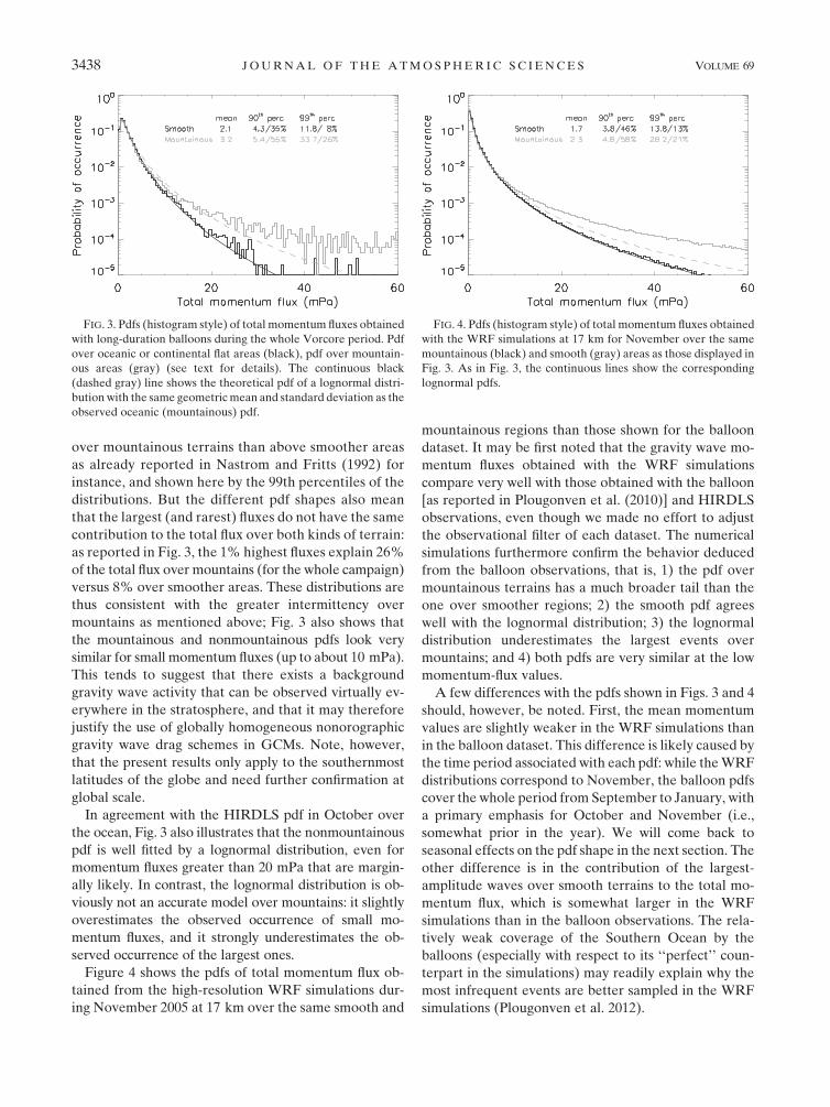
over mountainous terrains than above smoother areas

as already reported in Nastrom and Fritts (1992) for

instance, and shown here by the 99th percentiles of the

distributions. But the different pdf shapes also mean

that the largest (and rarest) fluxes do not have the same

contribution to the total flux over both kinds of terrain:

as reported in Fig. 3, the 1% highest fluxes explain 26%

of the total flux over mountains (for the whole campaign)

versus 8% over smoother areas. These distributions are

thus consistent with the greater intermittency over

mountains as mentioned above; Fig. 3 also shows that

the mountainous and nonmountainous pdfs look very

similar for small momentum fluxes (up to about 10 mPa).

This tends to suggest that there exists a background

gravity wave activity that can be observed virtually ev-

erywhere in the stratosphere, and that it may therefore

justify the use of globally homogeneous nonorographic

gravity wave drag schemes in GCMs. Note, however,

that the present results only apply to the southernmost

latitudes of the globe and need further confirmation at

global scale.

In agreement with the HIRDLS pdf in October over

the ocean, Fig. 3 also illustrates that the nonmountainous

pdf is well fitted by a lognormal distribution, even for

momentum fluxes greater than 20 mPa that are margin-

ally likely. In contrast, the lognormal distribution is ob-

viously not an accurate model over mountains: it slightly

overestimates the observed occurrence of small mo-

mentum fluxes, and it strongly underestimates the ob-

served occurrence of the largest ones.

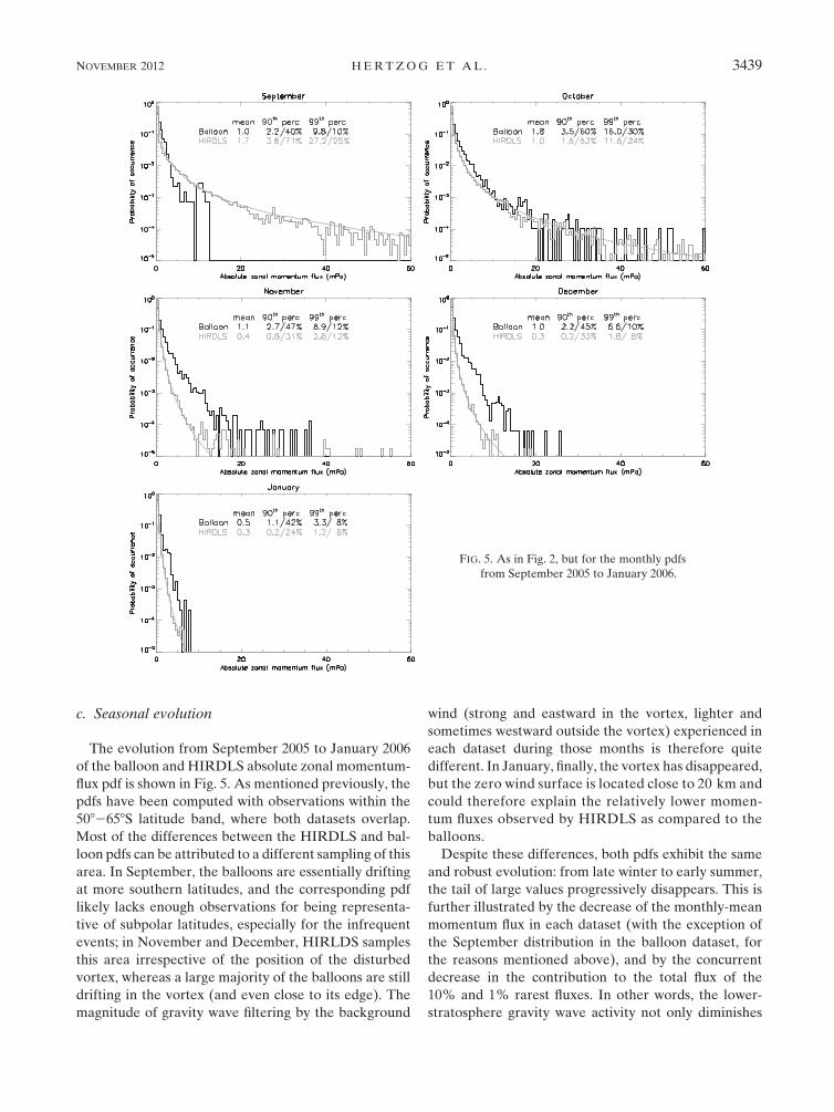
Figure 4 shows the pdfs of total momentum flux ob-

tained from the high-resolution WRF simulations dur-

ing November 2005 at 17 km over the same smooth and

mountainous regions than those shown for the balloon

dataset. It may be first noted that the gravity wave mo-

mentum fluxes obtained with the WRF simulations

compare very well with those obtained with the balloon

[as reported in Plougonven et al. (2010)] and HIRDLS

observations, even though we made no effort to adjust

the observational filter of each dataset. The numerical

simulations furthermore confirm the behavior deduced

from the balloon observations, that is, 1) the pdf over

mountainous terrains has a much broader tail than the

one over smoother regions; 2) the smooth pdf agrees

well with the lognormal distribution; 3) the lognormal

distribution underestimates the largest events over

mountains; and 4) both pdfs are very similar at the low

momentum-flux values.

A few differences with the pdfs shown in Figs. 3 and 4

should, however, be noted. First, the mean momentum

values are slightly weaker in the WRF simulations than

in the balloon dataset. This difference is likely caused by

the time period associated with each pdf: while theWRF

distributions correspond to November, the balloon pdfs

cover the whole period from September to January, with

a primary emphasis for October and November (i.e.,

somewhat prior in the year). We will come back to

seasonal effects on the pdf shape in the next section. The

other difference is in the contribution of the largest-

amplitude waves over smooth terrains to the total mo-

mentum flux, which is somewhat larger in the WRF

simulations than in the balloon observations. The rela-

tively weak coverage of the Southern Ocean by the

balloons (especially with respect to its ‘‘perfect’’ coun-

terpart in the simulations) may readily explain why the

most infrequent events are better sampled in the WRF

simulations (Plougonven et al. 2012).

FIG. 3. Pdfs (histogram style) of total momentum fluxes obtained

with long-duration balloons during the whole Vorcore period. Pdf

over oceanic or continental flat areas (black), pdf over mountain-

ous areas (gray) (see text for details). The continuous black

(dashed gray) line shows the theoretical pdf of a lognormal distri-

butionwith the same geometricmean and standard deviation as the

observed oceanic (mountainous) pdf.

FIG. 4. Pdfs (histogram style) of total momentum fluxes obtained

with the WRF simulations at 17 km for November over the same

mountainous (black) and smooth (gray) areas as those displayed in

Fig. 3. As in Fig. 3, the continuous lines show the corresponding

lognormal pdfs.


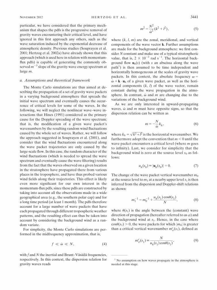
c. Seasonal evolution

The evolution from September 2005 to January 2006

of the balloon and HIRDLS absolute zonal momentum-

flux pdf is shown in Fig. 5. As mentioned previously, the

pdfs have been computed with observations within the

5082658S latitude band, where both datasets overlap.

Most of the differences between the HIRDLS and bal-

loon pdfs can be attributed to a different sampling of this

area. In September, the balloons are essentially drifting

at more southern latitudes, and the corresponding pdf

likely lacks enough observations for being representa-

tive of subpolar latitudes, especially for the infrequent

events; in November and December, HIRLDS samples

this area irrespective of the position of the disturbed

vortex, whereas a large majority of the balloons are still

drifting in the vortex (and even close to its edge). The

magnitude of gravity wave filtering by the background

wind (strong and eastward in the vortex, lighter and

sometimes westward outside the vortex) experienced in

each dataset during those months is therefore quite

different. In January, finally, the vortex has disappeared,

but the zero wind surface is located close to 20 km and

could therefore explain the relatively lower momen-

tum fluxes observed by HIRDLS as compared to the

balloons.

Despite these differences, both pdfs exhibit the same

and robust evolution: from late winter to early summer,

the tail of large values progressively disappears. This is

further illustrated by the decrease of the monthly-mean

momentum flux in each dataset (with the exception of

the September distribution in the balloon dataset, for

the reasons mentioned above), and by the concurrent

decrease in the contribution to the total flux of the

10% and 1% rarest fluxes. In other words, the lower-

stratosphere gravity wave activity not only diminishes

FIG. 5. As in Fig. 2, but for the monthly pdfs

from September 2005 to January 2006.


during this period over the Southern Ocean but also

becomes less and less intermittent. These two aspects

are likely caused by the progressive reversal of the zonal

wind that inhibits the upward propagation of a large

portion of the gravity wave spectrum.

d. Pdf evolution with height

Figure 6 displays the total momentum-flux pdfs in

WRF simulations at various heights over the whole

simulation domain. Although the WRF domain was

centered over the South Pole, it encompasses subpolar

latitudes so that the lowest altitudes shown are likely

partly located in the troposphere. These pdfs may thus

correspond to momentum fluxes that are not only as-

sociated with gravity wave disturbances but also tropo-

spheric processes (e.g., upper-level fronts).

With this reservation, the behavior of momentum-flux

pdfs with height is notably systematic in the WRF sim-

ulations. As one moves away from the tropospheric

gravity wave sources, the momentum fluxes regularly

decrease due to the progressive dissipation of the wave

field. But even more impressively, the pdf evolution

suggests self-similarity: the 90th and 99th percentiles

almost steadily correspond to 2 and 10 times the distri-

bution mean. Similarly, the contribution of the 10% and

1% rarest momentum fluxes amounts to about 50% and

15%–20%, respectively, of the total flux whatever the

altitude. In contrast with the seasonal evolution of the

pdfs, the November WRF simulations tend therefore

to show that the intermittency of the gravity wave mo-

mentum fluxes keeps constant with altitude (at least up

to the middle stratosphere).

Figure 7 displays the absolute momentum-flux pdfs

obtained with HIRDLS measurements at 20, 30, and

40 km. As HIRDLS observations do not cover latitudes

poleward of 658S, we have chosen for a better compar-

ison with the previous figure to show the HIRLDS pdfs

for September and October, which correspond to an

eastward circulation in the stratosphere at these sub-

polar latitudes as in November over the South Pole. The

magnitude and general height evolution of HIRDLS

pdfs compare very well with the WRF ones. Further-

more, as previously noted, the 90th percentile still rep-

resents about twice the mean momentum whatever the

altitude. In contrast, the main difference lies in the

contribution to the total flux of the 1% largest events,

which seems to decrease in the HIRDLS observations in

contrast with what was found in the numerical simula-

tions. Several factors may contribute to this difference.

Once again, the better sampling of the most infrequent

events in the WRF simulations could be one reason.

Besides, HIRDLS hardly resolves waves with hori-

zontal wavelengths smaller than about 400 km, which

are, on the contrary, explicitly resolved in the numer-

ical simulations. Finally, the vertical shear of the

stratospheric zonal wind is larger in September/October

than in November, which may result in an enhanced

wave filtering in the former months, and therefore

a decrease of the wave intermittency with height in the

HIRDLS pdfs.

4. Effect of filtering by the wind

In this section, we study with the help of Monte Carlo

simulations how the gravity wave filtering by the back-

ground flow is continuously modifying the shape of the

momentum-flux pdfs as the waves propagate upward in

the atmosphere. The following paragraphs will detail the

approach that we used, which has been inspired in many

respects by Hines (1993) and Souprayen et al. (2001). In

FIG. 6. Pdfs of total momentum fluxes obtained with the WRF

simulations at various heights for November. The pdfs are repre-

sentative of the whole simulation domain.

FIG. 7. Pdfs of absolute zonal momentum fluxes obtained with

HIRDLS observations at various heights between 508 and 658S in

September and October 2005.


particular, we have considered that the primary mech-

anism that shapes the pdfs is the progressive removal of

gravity waves encountering their critical level, and have

ignored in this first approach any others, such as the

wave saturation induced by the exponential decrease of

atmospheric density. Previous studies (Souprayen et al.

2001; Hertzog et al. 2002a) have already shown that this

approach (which is used here in relationwithmomentum-

flux pdfs) is capable of generating the commonly ob-

servedm23 slope of the gravity wave energy spectrum at

large m.

a. Assumptions and theoretical framework

The Monte Carlo simulations are thus aimed at de-

scribing the propagation of a set of gravity wave packets

in a varying background atmosphere that spreads the

initial wave spectrum and eventually causes the occur-

rence of critical levels for some of the waves. In the

following, we will neglect the nonlinear wave–wave in-

teractions that Hines (1991) considered as the primary

cause for the Doppler spreading of the wave spectrum;

that is, the modification of a given wave packet’s

wavenumbers by the resulting random wind fluctuations

caused by the whole set of waves. Rather, we will follow

the approach suggested in Souprayen et al. (2001), and

consider that the wind fluctuations encountered along

the wave packet trajectories are only caused by the

large-scale flow. In this case, the random character of the

wind fluctuations (which is needed to spread the wave

spectrum and eventually cause the wave filtering) results

from the fact that the waves observed on a given location

in the stratosphere have propagated there from various

places in the troposphere, and have thus probed various

wind fields along their trajectories. This effect is likely

even more significant for our own interest in the

momentum-flux pdfs, since these pdfs are constructed by

taking into account all the observations made in a wide

geographical area (e.g., the southern polar cap) and for

a long time period (at least 1 month). The pdfs therefore

account for a large number of wave packets that have

each propagated through different tropospheric weather

patterns, and the resulting effect can thus be taken into

account by considering the background wind as a ran-

dom variate.

For simplicity, the Monte Carlo simulations are per-

formed in the midfrequency approximation, that is,

f � v � N , (4)

with f andN the inertial and Brunt–Vasaila frequencies,

respectively. In this context, the dispersion relation for

gravity waves reads

m25N2

v2(k21 l2) , (5)

where (k, l, m) are the zonal, meridional, and vertical

components of the wave vector k. Further assumptions

are made for the background atmosphere: we first con-

sider N constant and make use of a typical stratospheric

value, that is, 2 3 1022 rad s21. The horizontal back-

ground flow uh(s) (with s an abscissa along the wave

path1) is then assumed to be time independent and

horizontally homogeneous at the scales of gravity wave

packets. In this context, the absolute frequency v5v1 k � uh of a given wave packet, as well as the hori-

zontal components (k, l) of the wave vector, remain

constant during the wave propagation in the atmo-

sphere. In contrast, v and m are changing due to the

variations of the background wind.

As we are only interested in upward-propagating

waves, v and m must have opposite signs, so that the

dispersion relation can be written as

m52N

vkh , (6)

where kh 5ffiffiffiffiffiffiffiffiffiffiffiffiffik2 + l2

pis the horizontal wavenumber. We

furthermore adopt the convention thatm, 0 until the

wave packet encounters a critical level (where m goes

to infinity). Last, we consider for simplicity that the

background wind is zero at the source level s0 as fol-

lows:

uh(s0)[ juh(s0)j5 0: (7)

The change of the wave packet vertical wavenumberm0

at the source level tom1 at a nearby upper level s1 is then

inferred from the dispersion and Doppler-shift relations

as shown:

m211 5m21

0 1uh(s1) cosu(s1)

N, (8)

where u(s1) is the angle between the (constant) wave

direction of propagation (hereafter referred to as u) andthe background wind at s1. Hence, in the case where

cosu(s1). 0, the wave packets for which jm0j is greaterthan a critical vertical wavenumber mc

u(s1), defined as

mcu(s1)[

N

uh(s1) cosu(s1), (9)

1 No assumption on how waves propagate in the atmosphere is

needed at this stage.


have encountered a critical level between s0 and s1. In

our numerical simulations, we will simply assume that

these wave packets are completely obliterated and that

consequently the totality of their momentum flux is no

longer in the wave field (but has been transferred to the

mean flow).

b. Monte Carlo simulations

Unless otherwise stated, the Monte Carlo simulations

of the momentum-flux pdfs proceed by starting from

a power-law spectral distribution of momentum flux

versus vertical wavenumber at the source level, that is,

uk9w9(m0)dm0 ;mb0dm0. The figures shown in the next

sections have thus been obtained with an initially flat

(b5 0) momentum-flux spectrum, which corresponds to

a kinetic energy spectrum uk92(m0) that scales as m0 at

low wavenumbers, as commonly reported in the atmo-

sphere (e.g., Fritts and VanZandt 1993). Simulations

with other momentum-flux source spectra have never-

theless been performed (with spectral laws varying from

b 5 21 to b 5 1), and provide essentially the same re-

sults. At the source level, this momentum flux is dis-

tributed within a range of vertical wavenumbers (from

jminfj to jmsupj), and the initial total momentum flux is

normalized in each numerical realization as shown:

r(s0)

ð2p0

ðjmsupj

jminfjuk9w9(m0)F(u) dm0 du5 1, (10)

where the function F(u) describes the angular de-

pendence in the horizontal plane of the source flux. This

uniform normalization is intended to represent a wave

source that emits gravity waves with always the same

momentum flux, that is, a perfectly nonintermittent

source. The evolution of the momentum-flux distribu-

tion during the wave propagation is thus entirely due to

the filtering of part of the initial spectrum by the back-

ground wind.

At each propagation step, the critical vertical wave-

number is computed according to Eq. (9), and the mo-

mentum flux associated with that part of the source

spectrum that has been filtered since the previous level is

set to 0. The remaining part is conservatively propagated

to the next level. The remaining flux after i propagation

steps is thus

F(si)5 r(s0)

ð2p0

ðmci,u

jminfjuk9w9(m0)F(u) dm0 du , (11)

where

mci,u [ min

j50...i[mc

u(sj)] (12)

is the minimum critical wavenumber between the source

level and the ith step of propagation for waves propa-

gating with an angle u with the zonal direction. [Equa-

tion (11) is only valid as long as the whole initial

spectrum has not be filtered, that is, as long as

mci,u . jminfj]. Hence, mc

i,u (through its dependence on

the background wind) exclusively carries the random

character of the momentum flux in the simulations.

Two different settings for the background wind have

beenused in theMonteCarlo simulations. Themomentum-

flux pdfs resulting from these two settings are described

in the following sections.

c. Simulation with a random wind field

In the first setting, designed to be as simple as possible,

the background wind is assumed to be unidirectional (e.g.,

zonal) and is generated with a discrete Gaussian white-

noise process: a set of independent and identically distrib-

uted normal randomvariables with zeromean and uniform

variance s2u. This mimics the approach used by Hines

(1993).2 By symmetry, we can then use aDirac distribution

for the angular dependence F(u)5 d(u 5 p); that is, the

waves propagate along only one direction of propagation,

colinear to the wind direction (e.g., westward). We have

used a standard deviation of su 5 7 m s21, and the initial

momentum flux is distributed between jminfj 5 0.1 cycles

per kilometer and jmsupj 5 1 cycles per kilometer, which

corresponds to phase speeds with respect to the ground

(ch 5 N/m) between 3 and 30 m s21. The probability of

filtering the whole wave field (uh . 30 m s21) is thus

marginal, as well as the probability of completely free

propagation (uh , 3 m s21). The following results are

based on 105 realizations of the background wind.

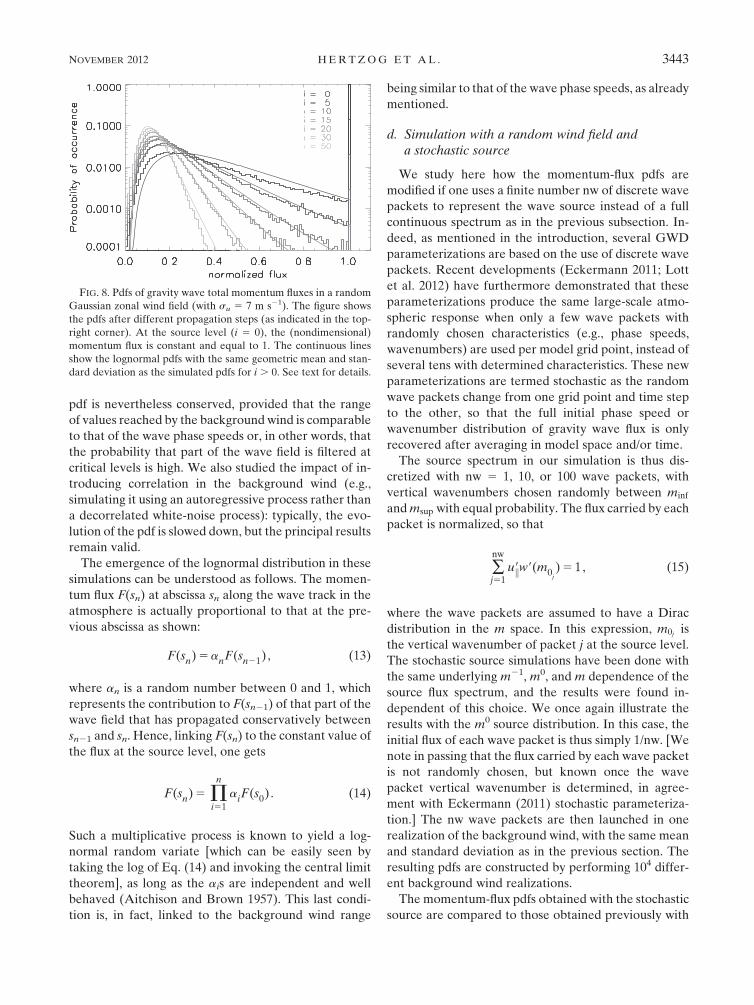
Figure 8 displays the evolution of the gravity wave

momentum-flux pdfs in this random wind field. The

initial single-valuemomentum flux is rapidly eroded due

to the efficient filtering by the background wind, and a

broad distribution quickly emerges. Most interestingly,

the resulting pdfs are consistent with the lognormal

distribution that appears in some observed pdfs after

about 10 propagation steps. Sensitivity tests have been

performed to assess how a change of the background

wind standard deviation modifies these results. As ex-

pected, a larger su produces distributions with smaller

fluxes, while a smaller su produces distributions with

larger fluxes. The general agreement with the lognormal

2 Note, in particular, that as in Hines (1993), the distance be-

tween two subsequent abscissas si and si11, which corresponds to

the ‘‘decorrelation distance’’ of the background wind along the

wave path, is left unspecified here. It would likely depend on the

wave tridimensionnal direction of propagation and on the local

atmospheric properties.


pdf is nevertheless conserved, provided that the range

of values reached by the backgroundwind is comparable

to that of the wave phase speeds or, in other words, that

the probability that part of the wave field is filtered at

critical levels is high. We also studied the impact of in-

troducing correlation in the background wind (e.g.,

simulating it using an autoregressive process rather than

a decorrelated white-noise process): typically, the evo-

lution of the pdf is slowed down, but the principal results

remain valid.

The emergence of the lognormal distribution in these

simulations can be understood as follows. The momen-

tum flux F(sn) at abscissa sn along the wave track in the

atmosphere is actually proportional to that at the pre-

vious abscissa as shown:

F(sn)5anF(sn21) , (13)

where an is a random number between 0 and 1, which

represents the contribution to F(sn21) of that part of the

wave field that has propagated conservatively between

sn21 and sn. Hence, linking F(sn) to the constant value of

the flux at the source level, one gets

F(sn)5Pn

i51

aiF(s0) . (14)

Such a multiplicative process is known to yield a log-

normal random variate [which can be easily seen by

taking the log of Eq. (14) and invoking the central limit

theorem], as long as the ais are independent and well

behaved (Aitchison and Brown 1957). This last condi-

tion is, in fact, linked to the background wind range

being similar to that of the wave phase speeds, as already

mentioned.

d. Simulation with a random wind field anda stochastic source

We study here how the momentum-flux pdfs are

modified if one uses a finite number nw of discrete wave

packets to represent the wave source instead of a full

continuous spectrum as in the previous subsection. In-

deed, as mentioned in the introduction, several GWD

parameterizations are based on the use of discrete wave

packets. Recent developments (Eckermann 2011; Lott

et al. 2012) have furthermore demonstrated that these

parameterizations produce the same large-scale atmo-

spheric response when only a few wave packets with

randomly chosen characteristics (e.g., phase speeds,

wavenumbers) are used per model grid point, instead of

several tens with determined characteristics. These new

parameterizations are termed stochastic as the random

wave packets change from one grid point and time step

to the other, so that the full initial phase speed or

wavenumber distribution of gravity wave flux is only

recovered after averaging in model space and/or time.

The source spectrum in our simulation is thus dis-

cretized with nw 5 1, 10, or 100 wave packets, with

vertical wavenumbers chosen randomly between minf

andmsup with equal probability. The flux carried by each

packet is normalized, so that

�nw

j51

uk9w9(m0j)5 1, (15)

where the wave packets are assumed to have a Dirac

distribution in the m space. In this expression, m0j is

the vertical wavenumber of packet j at the source level.

The stochastic source simulations have been done with

the same underlying m21, m0, and m dependence of the

source flux spectrum, and the results were found in-

dependent of this choice. We once again illustrate the

results with the m0 source distribution. In this case, the

initial flux of each wave packet is thus simply 1/nw. [We

note in passing that the flux carried by each wave packet

is not randomly chosen, but known once the wave

packet vertical wavenumber is determined, in agree-

ment with Eckermann (2011) stochastic parameteriza-

tion.] The nw wave packets are then launched in one

realization of the background wind, with the same mean

and standard deviation as in the previous section. The

resulting pdfs are constructed by performing 104 differ-

ent background wind realizations.

The momentum-flux pdfs obtained with the stochastic

source are compared to those obtained previously with

FIG. 8. Pdfs of gravity wave total momentum fluxes in a random

Gaussian zonal wind field (with su 5 7 m s21). The figure shows

the pdfs after different propagation steps (as indicated in the top-

right corner). At the source level (i 5 0), the (nondimensional)

momentum flux is constant and equal to 1. The continuous lines

show the lognormal pdfs with the same geometric mean and stan-

dard deviation as the simulated pdfs for i . 0. See text for details.


the full launch spectrum in Fig. 9. The resolution of the

latter pdf is, however, degraded with respect to that

shown in Fig. 8. Let us actually consider the case with

a single wave packet per wind realization (nw5 1). The

single wave packet carries the whole momentum flux,

and at propagation step i, the momentum flux can

therefore only take two values: 1 if the wave packet has

succeeded to propagate to this step from the source or

0 if it has been filtered in between. Turning back to the

general case, the momentum-flux pdfs can take nw 1 1

values in the stochastic source simulations. The full

launch spectrumpdfs are accordingly shown in Fig. 9 with

bin widths equal to 1/nw. Not surpringly, the nw 5 1

simulation is unable to reproduce the characteristics of

the momentum-flux distribution obtained with the full

launch spectrum. However, using 100 wave packets pro-

duces an excellent agreement with the spectral source.

One may also argue that the nw5 10 simulation starts to

retain essential features of the momentum-flux pdf (e.g.,

the broad tail), andmight therefore provide a good trade-

off between computational cost and momentum-flux in-

termittency in operational GWD parameterizations.

The ability of the stochastic source to generate

momentum-flux pdfs that more or less agree with those

obtained with the full spectral source tells, however,

nothing on how well the mean momentum flux, aver-

aged over all the random wind realizations, corresponds

to that obtained with the full spectral source. Figure 10

actually shows that, whatever the number nw of wave

packets in the stochastic source, the mean momentum

flux produced by the stochastic source is almost in-

distinguishable from that of the full spectral source. This

result mirrors the findings reported in Eckermann

(2011), who succeeded in obtaining a realistic mean-flow

forcing by running a stochastic GWD parameterization

with a single-wave packet source. In our simulations, this

result likely arises from both the large number of re-

alizations and the properties of the wave-filtering pro-

cess, which is constrained by the background wind

profile that has constant statistical characteristics. In

GCM runs, the large number of model grid points and

the ergodic character of the large-scale circulation may

provide companion agreements.

e. Simulation with a realistic wind field

To assess how the previous approach of the wave pdf

generation may work with more a realistic wind field,

FIG. 9. Pdfs of gravity wave total momentum fluxes in the ran-

dom Gaussian zonal wind field simulation. The panels show the

pdfs after different vertical propagation steps (as indicated in the

top-right corner of each panel). The pdfs produced by the ‘‘sto-

chastic source’’ are displayed with asterisks. The pdfs were ob-

tained by launching either (top) nw 5 1, (middle) nw 5 10, or

(bottom) nw5 100 wave packets per background wind realization.

The pdf obtained with the full launch spectrum (i.e., as in Fig. 8) is

displayed with continuous lines. The resolution of this pdf is

adapted to the number of wave packets used in the stochastic

source simulation (see text for details).

FIG. 10. Mean momentum flux remaining after the number of

propagation steps shown in the abscissa in the random wind sim-

ulation. The flux associated with the full launch spectrum source is

represented with a continuous line. Those corresponding to the

stochastic source are represented with dashed lines, and the gray

scale indicates the number of wave packets used.


another set of simulations has been performed with the

0000 UTC analyzed winds provided by the ECMWF

Integrated Forecast System. In this case, the analyses for

October 2010 south of 508S have been used, so as to

benefit from the highest possible resolution of the

model: 0.1258 3 0.1258 in the horizontal, 44 levels from

about 700 hPa (arbitrarily chosen as the source level) to

40 hPa in the vertical. The resulting pdfs are thus ob-

tained from about 9 3 105 individual simulations.

In the previous simulations with the random wind

field, we made the assumption that the wind values were

those felt by the waves during their propagation. Such an

approach could be reproduced with a realistic wind field

by performing ray-tracing simulations. However, to re-

duce the computation cost and to mimic what is cur-

rently done with GWD parameterizations, we simply

assumed here that the waves propagate vertically in the

atmosphere. In these ECMWF simulations, we fur-

thermore used an isotropic wave momentum flux at the

source, that is, F(u)5 1/2p. This isotropic source is

implemented by picking a single direction of propaga-

tion in a uniform distribution between 0 and 2p at each

ECMWF grid point. We otherwise used the same full

launch spectrum as in the random wind simulations,

except that we extended the range of the source wave-

numbers by using jminfj 5 0.05 cycles per kilometer and

jmsupj5 10 cycles per kilometer, corresponding to phase

speeds between 0.3 and 60 m s21.

The resulting pdfs are displayed in Fig. 11. As in the

random wind simulations, a broad momentum-flux pdf

with a shape that shares many similarities with the ob-

served ones is rapidly produced. Two features are

nonetheless different: first, despite the extended range

of ground-based phase speeds, the whole wave field is

able to propagate freely up to 40 hPa in a significant

number of individual simulations, as highlighted by the

pdf peak at F(si) 5 1. These simulations essentially

correspond to waves propagating toward the west in the

mainly eastward midlatitude October flow of the

Southern Hemisphere. Second, the agreement between

the produced pdfs and the lognormal distribution is only

obtained for the smallest momentum-flux values (up to

0.2–0.4). This last feature is also reminiscent of the ob-

served pdfs above mountainous areas in September/

October.

These two differences are associated with the fact that

the ECMWF wind field is, from the point of view of

wave filtering, less random than the one used in the first

simulation. In particular, themainly eastward flow in the

upper troposphere and the stratosphere implies that

ai 5 1 in Eq. (14) from a certain level onward for the

westward-propagating waves, so that the conditions for

the emergence of the lognormal distribution are no

longer met.

Simulations with a stochastic source (instead of the

full launch spectrum) in the ECMWF winds have been

performed too, and the results were found very similar

to those reported in the previous section: the pdf shape

displayed in Fig. 11 emerges with a relatively low num-

ber of wave packets (i.e., nw 5 10), while the mean

momentum flux does not depend on nw.

5. Summary and concluding remarks

The first part of this article was aimed at studying the

properties of gravity wave momentum-flux pdfs in the

upper troposphere and lower stratosphere over Ant-

arctica and the Southern Ocean. The pdfs have been

obtained independently from in situ balloonborne

measurements, limb-sounding observations of the at-

mosphere, and high-resolution numerical simulations.

In all these data sources, the momentum-flux pdfs ex-

hibit long tails that span over (at least) one or two orders

of magnitude, and therefore highlight the so-called in-

termittency of gravity wave activity in the lower strato-

sphere. It has been, for instance, shown that for the

region considered in this study, about 60% of the total

observed flux is only due to the 10% largest fluxes when

the winter regime of the stratospheric circulation is es-

tablished (and a large fraction of the waves can propa-

gate almost freely to the stratosphere). This figure is

even more pronounced above mountainous areas,

where typically 25% of the total flux is only produced by

1% of the events. We have also found that these char-

acteristics of the atmospheric gravity wave field keep

essentially constant with altitude, as long as the vertical

shear of the horizontal wind remains eastward in the

stratosphere. In contrast, the intermittency of gravity

wave activity decreases significantly during the transi-

tion from winter to summer circulation. While these

FIG. 11. As in Fig. 8, but for the simulations with the ECMWF

wind field.


features are found to be fairly robust whatever the da-

taset used, the characteristics of the momentum-flux

pdfs likely deserve to be further confirmed in other

places and seasons than those studied here. Using the

pdfs to assess the overall contribution of momentum

fluxes beyond certain percentiles as was done here [or to

compute a more synthetic metric, such as the Gini co-

efficient proposed by Plougonven et al. (2012)] actually

provides a useful way to quantify gravity wave in-

termittency.

The second part of this article described the role

played bywave filtering at critical levels inmodifying the

shape of momentum-flux pdfs. Simple Monte Carlo

simulations have been designed to study the propaga-

tion of gravity waves through a varying background

wind field. In the simulations with a random background

wind with values similar to those of the wave phase

speeds, the numerous occurrence of critical levels that

filter out a portion of the initial wave spectrum tends to

modify the single-value pdf used at the source level

(corresponding to a constant, homogeneous source)

toward lognormal pdfs, which are actually observed ei-

ther above oceanic areas during winter or summer. As

first suggested by Hines (1993), such evolution can be

understood as the multiplicative result of discrete fil-

tering events along the wave propagation, each event

corresponding to the deposition of a fraction of the re-

maining flux. In contrast, when the wind field is such that

a large portion of the gravity wave field can propagate

almost freely (as was the case in the simulations with the

November ECMWF-analyzed winds), significant de-

partures from the lognormal distribution are observed.

These departures are typically encountered in the ob-

servations above mountainous areas during winter (in

which case, the sporadic wave emission may also con-

tribute to the observed intermittency in the lower

stratosphere). These results were found to be rather

independent of how the wave source was treated, either

as a full spectrum or as a superposition of *10 in-

dependent wave packets. Finally, the limitations of our

simulations should be stressed: in particular, neither the

wave-induced fluctuations of the background wind nor

the saturation of individual wave packets were taken

into account. Both processes can enhance the deposition

of gravity wave momentum flux and therefore modify

the momentum-flux pdfs.

The sporadic gravity wave activity exemplified in this

article can provide some observational grounds for the

development and use of novel stochastic gravity wave

drag parameterizations in general circulation models

(e.g., Piani et al. 2004; Eckermann 2011; Lott et al. 2012).

But it may also be worthwhile to assess how the ob-

served gravity wave intermittency is simulated by

current deterministic GWD parameterizations. On the

one hand, one could expect that these parameterizations

simulate, at least to some extent, the filtering of the

gravity wave field by the background wind, which, as we

suggested, is an important factor in producing the ob-

served pdfs. On the other hand, most nonorographic

GWD parameterizations use a constant and/or homoge-

neous wave source, and therefore likely underestimate

the real wave intermittency. Such studywill be the subject

of future work.

Acknowledgments. The authors would like to ac-

knowledge CNES for the long-standing development of

stratospheric superpressure balloons and for the successful

Vorcore balloon campaign in 2005. The study benefited

from stimulating discussions at the International Space

Science Institute (ISSI) during the gravity wave group

meetings. We would like in particular to thank Julio

Bacmeister, Adam Scaife, andRobert A. Vincent for their

ideas and suggestions. This work was initiated during Joan

Alexander’s visit at LMD, which was funded by Ecole

Normale Superieure. The European Centre for Medium-

Range Weather Forecasts provided the meteorological

analyses used in this study. The WRF simulations were

performed on HPC resources from GENCI-IDRIS

(Grants 2009 and 2010-012039). Work by MJA was

supported by the NASA Atmospheric Chemistry-Aura

Science Team Program, Contract NNH11CD32C. The

authors would also like to thank two anonymous re-

viewers for their insightful remarks: the stochastic source

experiments were indeed performed according to one

reviewer’s suggestion.

REFERENCES

Aitchison, J., and J. A. C. Brown, 1957: The Lognormal Distribu-

tion, with Special Reference to Its Use in Economics. Cam-

bridge University Press, 176 pp.

Alexander, M. J., and L. Pfister, 1995: Gravity wave momentum

flux in the lower stratosphere over convection. Geophys. Res.

Lett., 22, 2029–2032.

——, and T. J. Dunkerton, 1999: A spectral parameterization of

mean-flow forcing due to breaking gravity waves. J. Atmos.

Sci., 56, 4167–4182.

——, and H. Teitelbaum, 2007: Observation and analysis of a large

amplitude mountain wave event over the Antarctic peninsula.

J. Geophys. Res., 112, D21103, doi:10.1029/2006JD008368.

——, and Coauthors, 2008: Global estimates of gravity wave mo-

mentum flux from High Resolution Dynamics Limb Sounder

observations. J. Geophys. Res., 113, D15S18, doi:10.1029/

2007JD008807.

——, S. D. Eckermann, D. Broutman, and J. Ma, 2009:Momentum

flux estimates for South Georgia Island mountain waves in the

stratosphere observed via satellite. Geophys. Res. Lett., 36,L12816, doi:10.1029/2009GL038587.

——, and Coauthors, 2010: Recent developments in gravity-wave

effects in climate models and the global distribution of


gravity-wave momentum flux from observations and models.

Quart. J. Roy. Meteor. Soc., 136, 1103–1124.

Andrews, D. G., J. R. Holton, and C. B. Leovy, 1987: Middle At-

mosphere Dynamics. Academic Press, 490 pp.

Baumgaertner, A. J. G., and A. J. McDonald, 2007: A gravity wave

climatology for Antarctica compiled from Challenging Min-

isatellite Payload/Global Positioning System (CHAMP/GPS)

radio occultations. J. Geophys. Res., 112,D05103, doi:10.1029/

2006JD007504.

Boccara, G., A. Hertzog, R. A. Vincent, and F. Vial, 2008: Esti-

mation of gravity wavemomentum flux and phase speeds from

quasi-Lagrangian stratospheric balloon flights. Part I: Theory

and simulations. J. Atmos. Sci., 65, 3042–3055.

Buhler, O., 2003: Equatorward propagation of intertia–gravity

waves due to steady and intermittent wave sources. J. Atmos.

Sci., 60, 1410–1419.

Dewan, E. M., 1997: Saturated-cascade similitude theory of gravity

wave spectra. J. Geophys. Res., 102 (D25), 29 799–29 817.

——, and R. E. Good, 1986: Saturation and the ‘‘universal’’ spec-

trum for vertical profiles of horizontal scalar winds in the at-

mosphere. J. Geophys. Res., 91 (D2), 2742–2748.

Eckermann, S. D., 2011: Explicitly stochastic parameterization of

nonorographic gravity wave drag. J. Atmos. Sci., 68, 1749–1765.——, and P. Preusse, 1999: Global measurements of stratospheric

mountain waves from space. Science, 286, 1534–1537.

Fritts, D. C., and W. Lu, 1993: Spectral estimates of gravity wave

energy and momentum fluxes. Part II: Parameterization of

wave forcing and variability. J. Atmos. Sci., 50, 3695–3713.

——, and T. E. VanZandt, 1993: Spectral estimates of gravity wave

energy and momentum fluxes. Part I: Energy dissipation, ac-

celeration, and constraints. J. Atmos. Sci., 50, 3685–3694.

——, T. Tsuda, S. Kato, T. Sato, and S. Fukao, 1988: Observa-

tional evidence of a saturated gravity wave spectrum in the

troposphere and lower stratosphere. J. Atmos. Sci., 45, 1741–

1759.

Gille, J., and Coauthors, 2008: High Resolution Dynamics Limb

Sounder: Experiment overview, recovery, and validation of ini-

tial temperature data. J.Geophys. Res., 113,D16S43, doi:10.1029/

2007JD008824.

Hertzog, A., and F. Vial, 2001: A study of the dynamics of the

equatorial lower stratosphere by use of ultra-long-duration

balloons 2. Gravity waves. J. Geophys. Res., 106 (D19),

22 745–22 761.

——, C. Souprayen, and A. Hauchecorne, 2002a: Eikonal simula-

tions for the formation and the maintenance of atmospheric

gravity wave spectra. J. Geophys. Res., 107, 4145, doi:10.1029/

2001JD000815.

——, F. Vial, C. R. Mechoso, C. Basdevant, and P. Cocquerez,

2002b: Quasi-Lagrangian measurements in the lower strato-

sphere reveal an energy peak associated with near-inertial

waves. Geophys. Res. Lett., 29, 1229, doi:10.1029/

2001GL014083.

——, and Coauthors, 2007: Strateole/Vorcore—Long-duration,

superpressure balloons to study the Antarctic lower strato-

sphere during the 2005 winter. J. Atmos. Oceanic Technol., 24,

2048–2061.

——, G. Boccara, R. A. Vincent, and F. Vial, 2008: Estimation of

gravity wave momentum flux and phase speeds from quasi-

Lagrangian stratospheric balloon flights. Part II:Results from the

Vorcore campaign in Antarctica. J. Atmos. Sci., 65, 3056–3070.Hines, C. O., 1991: The saturation of gravity waves in the middle

atmosphere. Part II: Development of Doppler-spread theory.

J. Atmos. Sci., 48, 1360–1379.

——, 1993: The saturation of gravity waves in the middle atmo-

sphere. Part IV: Cutoff of the incident wave spectrum.

J. Atmos. Sci., 50, 3045–3060.

——, 1997a: Doppler-spread parameterization of gravity-wave

momentumdeposition in themiddle atmosphere. Part 1: Basic

formulation. J. Atmos. Sol.-Terr. Phys., 59, 371–386.

——, 1997b: Doppler-spread parameterization of gravity-wave

momentum deposition in themiddle atmosphere. Part 2: Broad

and quasi monochromatic spectra, and implementation.

J. Atmos. Sol.-Terr. Phys., 59, 387–400.

Holton, J. R., 1983: The influence of gravity wave breaking on the

general circulation of the middle atmosphere. J. Atmos. Sci.,

40, 2497–2507.——, P. H. Haynes, M. E. McIntyre, A. R. Douglass, R. B. Hood,

and L. Pfister, 1995: Stratosphere-troposphere exchange. Rev.

Geophys., 33, 405–439.

Lindzen, R. S., 1981: Turbulence and stress owing to gravity wave

and tidal breakdown. J. Geophys. Res., 86 (C10), 9707–9714.

Lorenz, M. O., 1905: Methods of measuring the concentration of

wealth. Publ. Amer. Stat. Assoc., 9, 209–219.

Lott, F., L. Guez, and P. Maury, 2012: A stochastic parameteriza-

tion of non-orographic gravity waves: Formalism and impact

on the equatorial stratosphere. Geophys. Res. Lett., 39,

L06807, doi:10.1029/2012GL051001.

Medvedev, A. S., and G. P. Klaassen, 1995: Vertical evolution of

gravity wave spectra and the parameterization of associated

wave drag. J. Geophys. Res., 100 (D12), 25 841–25 853.

Morgenstern, O., and Coauthors, 2010: Review of the formulation

of present-generation stratospheric chemistry-climate models

and associated external forcings. J. Geophys. Res., 115,

D00M02, doi:10.1029/2009JD013728.

Nastrom, G.D., and K. S. Gage, 1985: A climatology of atmospheric

wavenumber spectra of wind and temperature observed by

commercial aircraft. J. Atmos. Sci., 42, 950–960.——, andD.C. Fritts, 1992: Sources ofmesoscale variability of gravity

waves. Part I: Topographic excitation. J. Atmos. Sci., 49, 101–110.

Pfister, L., and Coauthors, 1993: Gravity waves generated by

a tropical cyclone during the STEP tropical field program: A

case study. J. Geophys. Res., 98 (D5), 8611–8638.

Piani, C., W. A. Norton, and D. A. Stainforth, 2004: Equatorial

stratospheric response to variations in deterministic and sto-

chastic gravity wave parameterizations. J. Geophys. Res., 109,

D14101, doi:10.1029/2004JD004656.

Plougonven, R., A. Hertzog, and H. Teitelbaum, 2008: Observa-

tions and simulations of a large amplitude mountain wave

breaking over the Antarctic peninsula. J. Geophys. Res., 113,

D16113, doi:10.1029/2007JD009739.

——, A. Arsac, A. Hertzog, L. Guez, and F. Vial, 2010: Sensitivity

study for mesoscale simulations of gravity waves above Antarc-

tica during Vorcore.Quart. J. Roy. Meteor. Soc., 136, 1371–1377.

——,A.Hertzog, and L. Guez, 2012: Gravity wave overAntarctica

and the Southern Ocean: Consistent momentum fluxes in

mesoscale simulations and stratospheric balloon observations.

Quart. J. Roy. Meteor. Soc., doi:10.1002/qj.1965, in press.

Scinocca, J. F., 2003: An accurate spectral nonorographic gravity

wave drag parameterization for general circulation models.

J. Atmos. Sci., 60, 667–682.

Sidi, C., J. Lefrere, F. Dalaudier, and J. Barat, 1988: An improved

atmospheric buoyancy waves spectrum model. J. Geophys.

Res., 93 (D1), 774–790.

Skamarock, W., and Coauthors, 2008: A description of the Ad-

vanced ResearchWRF version 3. NCAR Tech. Note. NCAR/

TN-4751STR, 113 pp.


Smith, R. B., 1979: The influence of mountains on the atmosphere.

Advances in Geophysics, Vol. 21, Academic Press, 87–230.

Smith, S. A., D. C. Fritts, and T. E. VanZandt, 1987: Evidence for

a saturated spectrum of atmospheric gravity waves. J. Atmos.

Sci., 44, 1404–1410.

Souprayen, C., J. Vanneste, A. Hertzog, and A. Hauchecorne,

2001: Atmospheric gravity wave spectra: A stochastic

approach. J. Geophys. Res., 106 (D20), 24 071–24 086.

VanZandt, T. E., 1982: A universal spectrum of buoyancy waves in

the atmosphere. Geophys. Res. Lett., 9, 575–578.

——, andD. C. Fritts, 1989: A theory of enhanced saturation of the

gravity wave spectrum due to increases in atmospheric sta-

bility. Pure Appl. Geophys., 130, 399–420.

Vial, F., A. Hertzog, C. R. Mechoso, C. Basdevant, P. Cocquerez,

V. Dubourg, and F. Nouel, 2001: A study of the dynamics of the

equatorial lower stratospherebyuseofultra-long-durationballoons

1. Planetary scales. J. Geophys. Res., 106 (D19), 22 725–22 743.

Vincent, R. A., A. Hertzog, G. Boccara, and F. Vial, 2007: Quasi-

Lagrangian superpressure balloon measurements of gravity-

wave momentum fluxes in the polar stratosphere of both

hemispheres. Geophys. Res. Lett., 34, L19804, doi:10.1029/2007GL031072.

Warner, C. D., and M. E. McIntyre, 2001: An ultrasimple spectral

parameterization for nonorographic gravity waves. J. Atmos.

Sci., 58, 1837–1857.Watanabe, S.,Y.Kawatani,Y. Tomikawa,K.Miyazaki,M.Takahashi,

and K. Sato, 2008: General aspects of a T213L256 middle at-

mosphere general circulation model. J. Geophys. Res., 113,

D12110, doi:10.1029/2008JD010026.

Weinstock, J., 1990: Saturated andunsaturated spectraof gravitywaves

and scale-dependent diffusion. J. Atmos. Sci., 47, 2211–2225.

Wu, D. L., 2004: Mesoscale gravity wave variances from AMSU-A

radiances. Geophys. Res. Lett., 31, L12114, doi:10.1029/

2004GL019562.


on the intermittency of gravity wave momentum flux in the

Documents