on the control of time delay power … · international journal of innovative ... on the control of...

International Journal of InnovativeComputing, Information and Control ICIC International c©2013 ISSN 1349-4198Volume 9, Number 2, February 2013 pp. 769–792

ON THE CONTROL OF TIME DELAY POWER SYSTEMS

Muthana Taleb Alrifai1, Mohamed Zribi1, Mohamed Rayan1

and Magdi Sadiq Mahmoud2

1Department of Electrical EngineeringKuwait University

P.O. Box 5969, Safat, 13060, [email protected]

2Department of Systems EngineeringKing Fahd University of Petroleum and MineralsP.O. Box 985, Dhahran 31261, Saudi Arabia

Received December 2011; revised May 2012

Abstract. This paper deals with the control of a power system with time delay in thestates. The power system is a seventh order synchronous machine infinite bus system.The linearized model of the system belongs to a class of uncertain linear systems withstates delays. Two control schemes are proposed for the system. The first controlleruses only the instantaneous states for feedback; the second controller combines the effectsof the instantaneous as well as the delayed states. Using Lyapunov theory, it is proventhat both control schemes guarantee the exponential stabilization of the power system.Detailed simulation results clearly indicate that the proposed control schemes work well.Keywords: Power system, Delays in the state, Control

1. Introduction. Time delays are present in many physical systems [1]. These timedelays influence the stability of the systems and might degrade the performance of thesystem; hence they should be properly considered in the controller design [2,3].

Although time delay exists in the power system measurement and control loops, tra-ditional power system controllers were generally designed based on local information andtime delays were usually ignored. With the introduction of Wide-Area Measurement Sys-tem (WAMS) technology, synchronized real-time measurements are provided in the formof phasor measurement unit (PMU) which can be used for stability studies of power sys-tems. This leads to a more efficient controller design. However, time delays are presentsignificantly in these measurements due to transmission channels [3].

Several researchers worked on the control of power systems while considering the timedelay [2-41]. For example, in [4-8] the impact of time delay in the design of power systemstabilizers was discussed. An effective method to eliminate the oscillations introduced bytime-delayed feedback control was proposed in [9,10]. The work in [13] studied the effectsof inclusion of delays on the small signal stability of power systems. The researchers in[14] designed a control scheme using phasor measurements considering delays for smallsignal stability of power systems. The authors in [15] presented a wide-area control systemfor damping generator oscillations. Additional studies on the influence of time delay onpower system stability can be found in [11-41] and the references cited therein.

This paper contributes to the development of feedback controllers for power systemswith states delays. Motivated by the work in [42], two control schemes are proposedfor the system. The first controller uses only the instantaneous states for feedback; thesecond controller combines the effects of the instantaneous as well as the delayed states.

769

770 M. T. ALRIFAI, M. ZRIBI, M. RAYAN AND M. S. MAHMOUD

Using Lyapunov theory, it is proven that both control schemes guarantee the exponentialstabilization of the power system.The paper is organized as follows. The next section presents the dynamic model of

the power system. The control problem is formulated in Section 3. Section 4 presentsa robust feedback controller for uncertain linear systems with time delays in the states.Section 5 proposes a three term robust controller for the system. Detailed simulationresults of the controlled power system are presented and discussed in Section 6. Finally,some concluding remarks are given in Section 7.Notations. We use W t, W−1, λ(W ) to denote respectively, the transpose of, the

inverse of, and the eignvalues of any square matrix W . The vector norm is taken tobe the Euclidean norm and the matrix norm is the corresponding induced one; that is

‖W‖ = λ1/2M (W tW ), where λM(m)(W ) stands for the operation of taking the maximum

(minimum) eignvalue of W . We use W > 0 (W < 0) to denote a positive- (negative-)definite matrix W . We use xt to represent a segment of x(τ) on [t − η(t), t], that isxt : [−η(t), 0] → <n with ‖xt‖∗ = sup ‖x(τ)‖ with t− η∗ ≤ τ ≤ t. Let C−

o denote theproper left-half of the complex plane. Sometimes, the arguments of a function will beomitted in the analysis when no confusion can arise.

2. Dynamic Model of the Power System. A synchronous machine infinite bus powersystem is depicted in Figure 1. The dynamic model of the power system is derived in thissection. The symbols used in the description of the model are listed below.δ: the rotor angle with respect to the infinite bus system voltage,ωo: the synchronous angular speed,∆ω: the deviation of the rotor angular speed from the synchronous angular speed ωo,M : the effective inertia constant,Kd: the equivalent damping factor,E: the infinite bus voltage,Eq: the direct q-axis voltage,E ′

q: the transient q-axis voltage,Efd: the direct excitation voltage,E ′

fd: the transient excitation voltage,id: the d-axis current,T ′do: the equivalent transient rotor time constant,

xd: the d-axis reactance,x′d: the d-axis transient reactance,

xq: the q-axis reactance,xe: the reactance of the transmission lines,PM : the mechanical power,Pe: the electrical power,Vt: the terminal bus voltage,Vref : the reference voltage,∆V : the difference between the reference voltage and the terminal bus voltage,UPSS: the power system stabilizer (PSS) control signal,KA: the amplifier gain constant,TA: the amplifier time constant,y: the state of the governor system,G: the governor control signal.The dynamic model of the generator is described in terms of the following three first

order differential equations:

CONTROL OF TIME DELAY POWER SYSTEMS 771

δ = ωo∆ω (1)

∆ω =1

M(PM +G+Kd∆ω − Pe) (2)

E ′q =

1

T ′do

(Efd − (xd − x′

d)id − E ′q

)(3)

where

id =Eq − E cos δ

xe + xq

(4)

Eq = E ′q + (xd − x′

d)id (5)

Pe =E ′

qE sin δ

xe + x′d

(6)

Combining (4) and (5), one obtains,

id =E ′

q − E cos δ

xe + xq − xd + x′d

(7)

Figure 1. Block diagram of the electric power generation unit system

The following dynamic model for the Automatic Voltage Regulator (AVR) and theexciter is adopted:

Efd =KA

TA

(∆V + UPSS)−Efd

TA

(8)

where

∆V = Vref − Vt. (9)

The following dynamic model is considered for the governor:

y =1

Tg

(b∆ω(t− τ)− y) (10)

G = a∆ω(t− τ) + by. (11)


The dynamic model for the conventional power system stabilizer (PSS) is as follows:

z1 = z2 (12)

z2 = − T2

TQ

(z1 + (T2 + TQ)z2 −∆ω(t− τ)) (13)

and

UPSS = −KJ

KA

(−T1

T2

z1 +(TQ − T1T2 − T1TQ)

T2

z2 +T1

T2

∆ω(t− τ)

). (14)

The overall model of the power system is given by the above equations. From theabove equations, it can be seen that the model of the power system is of order 7 and itis nonlinear with state delays. To be able to analyze and control the power system, themodel is linearized around the operating point (δo, ωo, E

′qo , Efdo , yo, z1o, z2o).

Let ∆δ = δ − δo, ∆ω = ω − ωo, ∆E ′q = E ′

q − E ′qo , ∆Efd = Efd − Efdo , ∆y = y − yo,

∆z1 = z1 − z1o and ∆z2 = z2 − z2o. Therefore, the linearized model of the power systemcan be written as:

∆δ = ωo∆ω

∆ω =1

M(∆PM +∆G+Kd∆ω −∆Pe)

∆E ′q =

1

T ′do

(∆Efd − (∆E ′

q + E sin δo∆δ)xd − x′

d


−∆E ′q

)∆Efd =

KA

TA

(∆V +∆UPSS)−∆Efd

TA

∆y =1

Tg

(b∆ω(t− τ)−∆y)

∆z1 = ∆z2

∆z2 = − 1

T2TQ

(∆z1 + (T2 + TQ)∆z2 −∆ω(t− τ))

(15)

Further manipulations of the above model yield:

∆δ = ωo∆ω

∆ω =1

M

(∆PM + a∆ω(t− τ) + b∆y +Kd∆ω −

E ′qoE sin δo

xe + x′d

∆E ′q

−E ′

qoE cos δo

xe + x′d

∆δ

)∆E ′

q =1

T ′do

(∆Efd −

xe + xq


∆E ′q − E sin δo

xd − x′d


∆δ

)∆Efd =

KA

TA

(∆V +

KJT1

KAT2

∆z1 −KJ(TQ − T1T2 − T1TQ)

KAT2

∆z2

−KJT1

KAT2

∆ω(t− τ)

)− ∆Efd

TA

∆y =1

Tg

(b∆ω(t− τ)−∆y)

∆z1 = ∆z2

∆z2 = − 1

T2TQ

(∆z1 + (T2 + TQ)∆z2 −∆ω(t− τ))

(16)


The outputs of the system are taken to be the deviation of the rotor angle and thedeviation of the rotor angular speed.

Define the states and the inputs of the power system such that:

x =(∆δ ∆ω ∆E ′

q ∆Efd ∆y ∆z1 ∆z2)t

and u = (∆PM ∆V )t

Hence, the linearized model of the power system can be written in a compact form as,

x(t) = Aox(t) +Bou(t) +Dx(t− τ) + ζ(x, t)

z(t) = Eox(t)(17)

where

Ao =

0 ωo 0 0 0 0 0K1 Kd/M K2 0 b/M 0 0K3 0 K4

1T ′do

0 0 0

0 0 0 −1TA

0 K5 K6

0 0 0 0 −1Tg

0 0

0 0 0 0 0 0 10 0 0 0 0 K7 K8

, D =

0 0 0 0 0 0 00 a/M 0 0 0 0 00 0 0 0 0 0 00 K9 0 0 0 0 00 K10 0 0 0 0 00 0 0 0 0 0 00 K11 0 0 0 0 0

Bo =

0 01M

00 00 KA

TA

0 00 00 0

, Eo =

[1 0 0 0 0 0 00 1 0 0 0 0 0

]

and, the parameters K1-K11 are defined such that:

K1 = −E ′

qoE cos δo

M(xe + x′d)

K2 = −E ′

qoE sin δo

M(xe + x′d)

K3 = −E sin δoxd − x′

d

T ′do(xe + xq − xd + x′

d)

K4 = − xe + xq

T ′do(xe + xq − xd + x′

d)

K5 =KJ T1

TA T2

K6 =−KJ(TQ − T1T2 − T1TQ)

TA T2

K7 =−1

T2 TQ

K8 = −T2 + TQ

T2 TQ

K9 = −KJ T1

TA T2


K10 =b

Tg

K11 =1

T2 TQ

Note that the term ζ(x, t) is added in (17) to represent the external disturbances actingon the system. System (17) belongs to the general class of uncertain linear systems withstate delays. The next three sections deal with the formulation and the design of controlschemes for this class of systems.

3. Formulation of the Control Problem. Consider a class of dynamical systems withtime-varying state-delay of the form:

x(t) = Aox(t) +Bou(t) +Dx(t− η(t)) + ζ(x, t) (18)

0 ≤ η(t) ≤ η∗ and η(t) ≤ η+ < 1

x(t) = %d(t) for t ∈ [−η∗, 0]

where t ∈ < is the time, x ∈ <n is the instantaneous state; u ∈ <m is the control input.The variable η(t) represents the delay of the system with bounds η∗ and η+ which areassumed to be known. The matrices Ao ∈ <n×n, Bo ∈ <n×m, represent the nominalsystem. The uncertainties within the system are represented by a delay factor multipliedby the matrix D and a current factor contained in the nonlinear vector ζ(x, t).

Remark 3.1. The assumption that η(t) ≤ η+ < 1 stems from the need to bound the growthvariations in the delay factor as a time-function. This assumption can be considered quiterealistic and holds for a wide class of uncertain dynamical systems. Thus our designresults are applicable for the class of linear time-delay systems with bounded state-delayin the manner of (18).

Definition 3.1. The uncertain state-delay system (18) is said to be robustly stable ifthe solution x(t) = 0 of system (18) with u(t) = 0 is uniformly asymptotically stable forall admissible realizations of the uncertainties D and ζ(., .).

Definition 3.2. The uncertain state-delay system (18) is said to be robustly stabiliz-able with a degree of stability γ > 0 if there exists a feedback control u[x(t)] such thatthe resulting closed-loop system is robustly stable and the solution of the controlled systemsatisfies:

‖x(τa)‖ ≤ ‖x(τb)‖ exp (−γ(τa − τb)) ∀τa ≥ τb ∈ <+. (19)

Assumptions:The following structural and growth constraints on ζ(., .) and D are considered.A1. There exist sufficiently smooth functions h(.) : <n×< → <m and g(.) : <n×< →

<n, such that:ζ(x, t) = Boh(x, t) + g(x, t) ∀(x, t) ∈ <n ×< (20)

A2. There exist positive constants α and β such that:

‖h(x, t)‖ ≤ α‖x(t)‖‖g(x, t)‖ ≤ β‖x(t)‖ (21)

A3. There exist functions G ∈ <m×n and L ∈ <n×n such that:

D = BoG+ L (22)

A4. Suppose that λ(Ao) ∈ C−o . It follows that there exist matrices 0 < P = P t ∈ <n×n

and 0 < Q = Qt ∈ <n×n such that for some κ > 0,

P (Ao + κI) + (Ao + κI)tP = −Q (23)


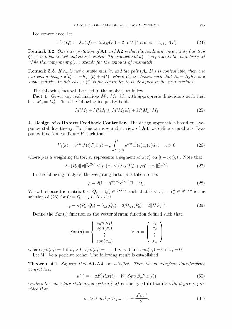
For convenience, let

σ(P,Q) := λm(Q)− 2βλM(P )− 2‖LtP‖2 and ω = λM(GGt) (24)

Remark 3.2. One interpretation of A1 and A2 is that the nonlinear uncertainty functionζ(., .) is mismatched and cone-bounded. The component h(., .) represents the matched partwhile the component g(., .) stands for the amount of mismatch.

Remark 3.3. If Ao is not a stable matrix, and the pair (Ao, Bo) is controllable, then onecan easily design u(t) = −Ksx(t) + v(t), where Ks is chosen such that Ao − BoKs is astable matrix. In this case, v(t) is the controller to be designed in the next sections.

The following fact will be used in the analysis to follow.Fact 1. Given any real matrices M1, M2, M3 with appropriate dimensions such that

0 < M3 = M t3. Then the following inequality holds:

M t1M2 +M t

2M1 ≤ M t1M3M1 +M t

2M−13 M2 (25)

4. Design of a Robust Feedback Controller. The design approach is based on Lya-punov stability theory. For this purpose and in view of A4, we define a quadratic Lya-punov function candidate V1 such that,

V1(x) = e2κtxt(t)Pox(t) + ρ

∫ t

t−η(t)

e2κτxtt(τ)xt(τ)dτ ; κ > 0 (26)

where ρ is a weighting factor; xt represents a segment of x(τ) on [t− η(t), t]. Note that

λm(Po)‖x‖2e2κt ≤ V1(x) ≤ (λM(Po) + ρη∗) ‖xt‖2∗e2κt. (27)

In the following analysis, the weighting factor ρ is taken to be:

ρ = 2(1− η+)−1e2κη∗(1 + ω). (28)

We will choose the matrix 0 < Qo = Qto ∈ <n×n such that 0 < Po = P t

o ∈ <n×n is thesolution of (23) for Q = Qo + ρI. Also let,

σo = σ(Po, Qo) = λm(Qo)− 2βλM(Po)− 2‖LtPo‖2. (29)

Define the Sgn(.) function as the vector signum function defined such that,

Sgn(σ) =

sgn(σ1)sgn(σ2)

...sgn(σm)

∀ σ =

σ1

σ2...σm

where sgn(σi) = 1 if σi > 0, sgn(σi) = −1 if σi < 0 and sgn(σi) = 0 if σi = 0.

Let W1 be a positive scalar. The following result is established.

Theorem 4.1. Suppose that A1-A4 are satisfied. Then the memoryless state-feedbackcontrol law:

u(t) = −µBtoPox(t)−W1Sgn(B

toPox(t)) (30)

renders the uncertain state-delay system (18) robustly stabilizable with degree κ pro-vided that,

σo > 0 and µ > µo = 1 +α2σ−1

o

2. (31)


Proof: The time derivative of the Lyapunov function candidate V1(.) in (26) evaluatedalong the trajectories of (18) is given by,

V1(x) = e2κt [xt(t)Pox(t) + xt(t)Pox(t) + 2κxt(t)Pox(t)+ρxt(t)x(t)− ρe−2κη(1− η)xt(t− η)x(t− η)]

= e2κt [xt(t) (Po(Ao + κI) + (Ao + κI)tPo + ρI) x(t) + 2xt(t)PoBou(t)+2xt(t)Poζ(x, t) + 2xt(t)PoDx(t− η)− ρe−2κη(1− η)xt(t− η)x(t− η)]

(32)

By substituting (20), (22), (23) and (30) into (32), we get

V1(x) = e2κt[−xt(t)Qox(t)− 2µxt(t)PoBoB

toPox(t)− 2W1x

t(t)PoBoSgn(BtoPox(t))

+2xt(t)Poζ(x, t) + 2xt(t)PoDx(t− η)− ρe−2κη(1− η)xt(t− η)x(t− η)]

= e2κt[−xt(t)Qox(t)− 2µxt(t)PoBoB

toPox(t)− 2W1x

t(t)PoBoSgn(BtoPox(t))

+ 2xt(t)Po (Boh+ g) + 2xt(t)Po (BoG+ L)x(t− η)

−ρe−2κη(1− η)xt(t− η)x(t− η)]

(33)

Algebraic manipulation of (33) yields:

V1(x) ≤ e2κt[−λm(Qo)‖x(t)‖2 − 2µ‖Bt

oPox‖2 + 2xt(t)PoBoh+ 2xt(t)Pog

+ 2xt(t)PoBoGx(t− η) + 2xt(t)PoLx(t− η)

−ρe−2κη∗(1− η+)xt(t− η)x(t− η)] (34)

Application of Fact 1 to (34), using (21) and rearranging terms gives:

V1(x) ≤ e2κt[−λm(Qo)‖x(t)‖2 − 2µ‖Bt

oPox‖2 + 2α‖BtoPox‖, ‖x‖+ 2βλM(Po)‖x‖2

+ 2xt(t)PoBoBtoPox(t) + 2xt(t− η)GtGx(t− η) + 2xt(t)PoLL

tPox(t)

+ 2xt(t− η)x(t− η) −ρe−2κη∗(1− η+)xt(t− η)x(t− η)]

≤ e2κt[−λm(Qo)− 2βλM(Po)− 2‖LtPo‖2

‖x‖2 − 2 (µ− 1) ‖Bt

oPox‖2

+ 2 α‖BtoPox‖ ‖x‖+

(2 + 2ω − ρe−2κη∗(1− η+)

)‖x(t− η)‖2

](35)

Using (28), we get from (35) the inequality:

V1(x) ≤ −e2κt(‖x‖ ‖Bt

oPox‖)Ω1

(‖x‖

‖BtoPox‖

)(36)

Ω1 =

[σo −α−α 2(µ− 1)

]It is readily seen that the positive-definiteness of Ω1 is satisfied when:

σo > 0 and 2 (µ− 1)σo > α2. (37)

Simple rearrangement of (37) entails conditions (31). Therefore, we have for all realiza-tions of uncertainties and ∀t ∈ <, x ∈ <n, the Lyapunov stability condition:

V1(x) ≤ −εe2κt ‖x‖2 ≤ 0 for ε > 0. (38)

By (20)-(22), the solution of the controlled uncertain system (18) is given by:

x(t) =(Ao − µBoB

toPo

)x(t) +Bo (h(x, t) +Gx(t− η))

+ g(x, t) + Lx(t− η)−W1BoSgn(BtoPox(t)).

(39)


From the previous analysis, it can be concluded that the solution of (39) satisfies thestate-norm inequality

‖x(τ)‖ ≤

√λM(Po) + ρη∗

λm(Po)‖x(ξ)‖ e−κ(τ−ξ), ∀τ ≥ ξ. (40)

In turn, this implies that,

‖x(τ)‖∗ ≤

√λM(Po) + ρη∗

λm(Po)‖x(ξ)‖∗ e−κ(τ−ξ) , ∀τ ≥ ξ. (41)

Therefore, we conclude that system (18) is robustly stabilizable by controller (30) andhas a degree of stability κ > 0.

Remark 4.1. The term −W1Sgn(BtoPox(t)) is added to the control law in (30) because

it is expected that this term will enhance the robustness of the closed loop system.

Remark 4.2. The case of constant delay where η(t) = η∗ = d and hence η = 0 can beeasily obtained from the previous result. In this case, the dynamic model is given by:

x(t) = Aox(t) +Bou(t) +Dx(t− d) + ζ(x, t) (42)

and we use the proposed controller for robust feedback synthesis based on the Lyapunovfunction (26). In this case, set

ρ∗ = 2e2κd(1 + ω) (43)

and choose a matrix 0 < Q∗ = Qt∗ ∈ <n×n such that 0 < P∗ = P t

∗ ∈ <n×n is the solutionof (23) for Q = Q∗ + ρ∗I. Define

σ∗ = σ(P∗, Q∗) := λm(Q∗)− 2βλM(P∗)− 2‖LtP∗‖2 (44)

Therefore, we obtain the following corollary for W1 > 0.

Corollary 4.1. Suppose that A1-A4 are satisfied. Then the control law:

u(t) = −µBtoP∗x(t)−W1Sgn(B

toP∗x(t))

renders the uncertain system (42) robustly stabilizable with a degree κ provided that

σ∗ > 0, µ > µ∗ = 1 +α2σ−1

∗2

(45)

The proof follows the procedure of Theorem 4.1.

5. Design of a Robust Feedback Controller with a Delay Term. Now, we considerthe case of constant delay where η(t) = η∗ = d and hence η = 0. In this case the dynamicmodel of the system is given by,

x(t) = Aox(t) +Bou(t) +Dx(t− d) + ζ(x, t). (46)

Let W2 be a positive scalar. We now propose the controller,

u(t) = −µBtoP x(t) + Kx(t− d)−W2Sgn(B

toP x(t)) (47)

which combines the effect of the instantaneous as well as the delay states. This controllerprovides three degrees of freedom: one by the proportional term −µBt

oP x(t) and the otherthrough the delay term Kx(t− d) and the third through −W2Sgn(B

toP x(t)) term. Note

that the third term is used to enhance the robustness of the closed loop system.To study the stability behavior in this case, we define a quadratic Lyapunov function

candidate as

V2(x) = e2κtxt(t)P x(t) +

∫ t

t−d

e2κτxtt(τ)xt(τ)dτ ; κ > 0 (48)


Choose a matrix 0 < Q = Qt ∈ <n×n such that 0 < P = P t ∈ <n×n is the solution of (23)for Q+ I. Let

σ = σ(P , Q) := λm(Q)− 2βλM(P )− 2‖LtP‖2 (49)

ζ = 2(µ− 2) and v = −2(1 + ω) + e−2κd (50)

The stability behavior is established by the following theorem.

Theorem 5.1. Suppose that A1-A4 are satisfied. Then the proportional-delay feedbackcontrol (47) renders the uncertain system (46) robustly stabilizable with degree κ > 0provided that

λm(Q) > 2βλM(P ) + 2‖LtP‖2 (51)

µ > µ = 2 +α2σ−1

2, (52)

‖K‖ < k =√v/2. (53)

Proof: The time derivative of the Lyapunov function candidate V2(.) evaluated alongthe solutions of system (46) while using the controller (47) is given by,

V2(x) = e2κt[xt(t)P x(t) + xt(t)P x(t) + 2κxt(t)P x(t) + xt(t)x(t)

−e−2κdxt(t− d)x(t− d)]

= e2κt[xt(t)

(P (Ao + κI) + (Ao + κI)tP + I

)x(t)− 2µxt(t)PBoB

toP x(t)

+2xt(t)PBoKx(t− d)− 2W2xt(t)PBoSgn(B

toP x(t)) + 2xt(t)P ζ(x, t)

+2xt(t)PDx(t− d)− e−2κdxt(t− d)x(t− d)]

(54)

By substituting (20), (22) and (23) into (54), we get,

V2(x) ≤ e2κt[−λm(Q)‖x(t)‖2 − 2µ‖Bt

oP x‖2 + 2xt(t)PBoKx(t− d)

+2xt(t)PBoh+ 2xt(t)P g + 2xt(t)PBoGx(t− d) + 2xt(t)PLx(t− d)

−e−2κdxt(t− d)x(t− d)] (55)

Application of Fact 1 to (55) and rearranging terms gives:

V2(x) ≤ e2κt[−λm(Q)‖x(t)‖2 − 2µ‖Bt

oP x‖2 + 2xt(t)PBoBtoP x(t)

+2xt(t− d)KtKx(t− d) + 2α‖BtoP x‖ ‖x‖+ 2βλM(P )‖x‖2

+2xt(t)PBoBtoP x(t) + 2xt(t− d)GtGx(t− d)

+2xt(t)PLLtP x(t) + 2xt(t− d)x(t− d)− e−2κdxt(t− d)x(t− d)]

≤ e2κt[−λm(Q)− 2βλM(P )− 2‖LtP‖2

‖x‖2 − 2 (µ− 2) ‖Bt

oP x‖2+2α‖Bt

oP x‖ ‖x‖+(2 + 2ω + 2‖K‖2 − e−2κd

)‖x(t− d)‖2

]≤ e2κt

[−σ ‖x‖2 − ζ ‖Bt

oP x‖2 + 2α‖BtoP x‖ ‖x‖

−(υ − 2‖K‖2

)‖x(t− d)‖2

](56)

Upon using (49) we get the inequality:

V2(x) ≤ −e2κt(‖x‖ ‖Bt

oP x‖ ‖x(t− d)‖)Ω2

‖x‖‖Bt

oP x‖‖x(t− d)‖

(57)

where,

Ω2 =

σ −α 0−α ζ 00 0 υ − 2‖K‖2

.


The positive definiteness of Ω2 is satisfied when

σ > 0, σζ − α2 > 0 and υ − 2‖K‖2 > 0 (58)

Algebraic manipulation of (58) in view of (49) and (50) gives immediately conditions(51)-(53). Therefore, we have for all realizations of uncertainties and ∀t ∈ <, ∀x ∈ <n

the Lyapunov stability condition:

V2(x) ≤ −εe2κt‖x‖2 ≤ 0 (59)

is satisfied for some ε > 0. The remaining part is obtained in a similar manner to theproof of Theorem 4.1.

6. Simulation Results. The controllers proposed in the previous two sections are ap-plied to the power system presented in Section 2. The performances of the system aresimulated using the MATLAB software. The numerical parameters of the power systemare given as follows.

The parameters of the synchronous machine are:

ωo = 314.16rad./sec. M = 6.92 Kd = −0.027xd = 1.24p.u. xq = 0.743p.u. x′

d = 0.022p.u.xe = 0.8p.u. PM = 0.437p.u. E = 1.0p.u.T ′d0 = 5.0sec. δo = 20o E ′

qo = 1.05p.u.

The parameters of the AVR and excitation system are:

KA = 250 TA = 0.001sec. Vref = 1.0p.u.

The parameters of the governor system are:

a = −0.001238 b = −0.17 Tg = 0.25sec.

The parameters of the conventional PSS are:

KJ = 12 TQ = 2.5sec. T1 = 0.1sec. T2 = 0.03sec.

The initial condition of the system is taken as, xo = [0.7859 0 1.0291 1.2075 0 0 0].The time delay τ is 0.7. It should be noted that since the delay factor τ occurs in thedynamics of the governor and the PSS, it can be estimated using off-line computation. Thedisturbance used is ζ(t) = [sin (2πft) cos (2πft) sin (2πft) cos (2πft) sin (2πft)cos (2πft) sin (2πft)] with f = 50Hz.

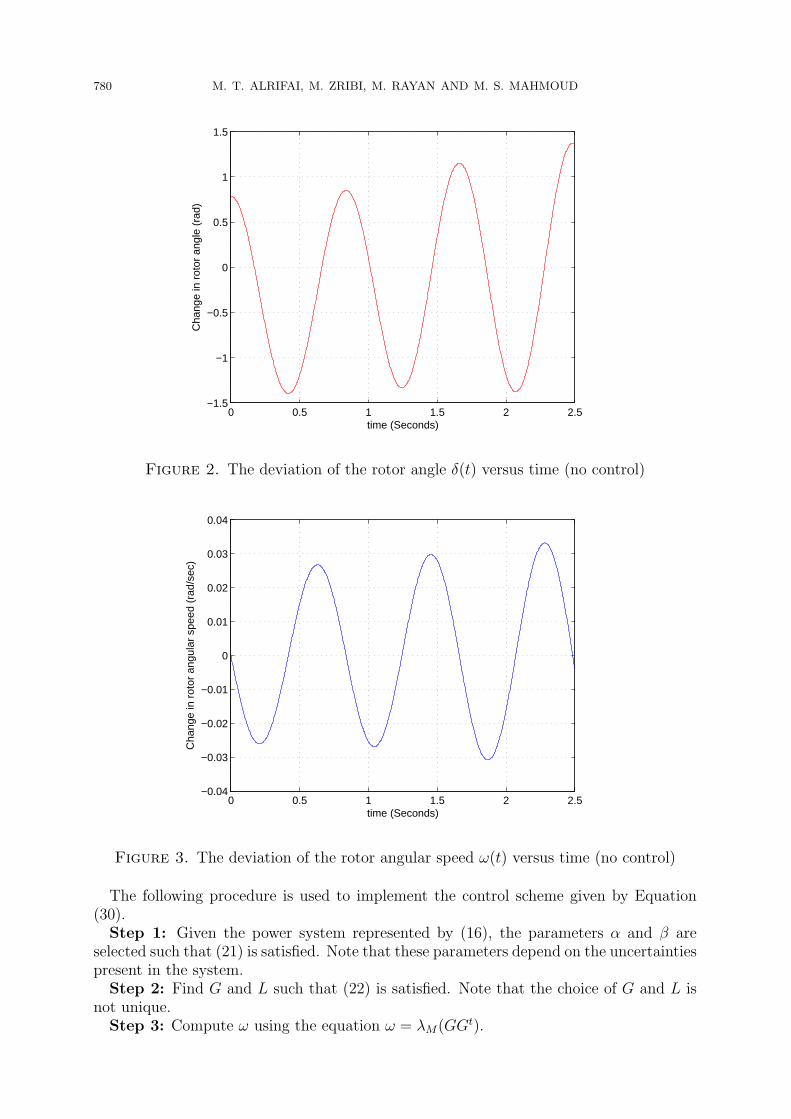
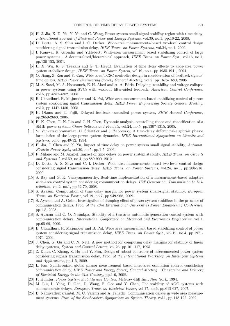
To show the need for controlling the power system with delays in the states, the lin-earized model of the system given by (16) is simulated when the time delay τ = 0.7. Thesimulation results are presented in Figures 2-4. Figure 2 shows the deviation of the rotorangle versus time; Figure 3 depicts the deviation of the rotor angular speed versus time.Figure 4 shows the deviation of the direct q-axis voltage versus time. It is clear from thesefigures that the uncontrolled system is unstable.

6.1. Simulation results of the power system controlled using the first controlscheme. This subsection presents the simulation results of the power system when itis controlled using the control scheme given by Equation (30). The parameters of thecontroller are taken to be µ = 0.08 and W1 = 0.8.

Since the proposed controller assumes that the system matrix Ao is a stable matrix,the MATLAB command eig is used to compute the eigenvalues of Ao. The eigenvalues ofAo are found to be [−0.048+ j7.377,−0.048− j7.377,−0.857,−1000,−33.33,−0.4,−4.0]where j2 = −1. Therefore, the matrix Ao is a stable matrix and the required condition issatisfied.


0 0.5 1 1.5 2 2.5−1.5

−1

−0.5

0

0.5

1

1.5

time (Seconds)

Cha

nge

in r

otor

ang

le (

rad)

Figure 2. The deviation of the rotor angle δ(t) versus time (no control)

0 0.5 1 1.5 2 2.5−0.04

−0.03

−0.02

−0.01

0

0.01

0.02

0.03

0.04

time (Seconds)

Cha

nge

in r

otor

ang

ular

spe

ed (

rad/

sec)

Figure 3. The deviation of the rotor angular speed ω(t) versus time (no control)

The following procedure is used to implement the control scheme given by Equation(30).Step 1: Given the power system represented by (16), the parameters α and β are

selected such that (21) is satisfied. Note that these parameters depend on the uncertaintiespresent in the system.Step 2: Find G and L such that (22) is satisfied. Note that the choice of G and L is

not unique.Step 3: Compute ω using the equation ω = λM(GGt).


0 0.5 1 1.5 2 2.5−0.8

−0.6

−0.4

−0.2

0

0.2

0.4

0.6

0.8

1

1.2

time (Seconds)

Cha

nge

in E

q (p

u V

olta

ge)

Figure 4. The deviation of the direct q-axis voltage Eq(t) versus time (no control)

0 0.5 1 1.5 2 2.5−0.5

0

0.5

1

time (Seconds)

Cha

nge

in r

otor

ang

le (

rad)

Figure 5. The deviation of the rotor angle δ(t) versus time (first controller)

Step 4: Select κ; one should start with a small value of κ and then increase this valueincrementally. Note that κ represents some sort of stability margin.

Step 5: Using the bounds η∗ and η+, compute ρ from Equation (28). For constanttime delay τ , η∗ = η = τ and η+ = 0

Step 6: Choose Qo > 0 such that Po is the solution of (23) with Q = Qo + ρI.Step 7: Compute σo using Equation (29).Step 8: Choose µ such that (31) is satisfied.Step 9: Simulate and analyze the performance of the system when the memoryless

state-feedback controller (30) is used.


At first, the system is simulated assuming that the system has no uncertainties. Thesimulation results are presented in Figures 5-7. Figure 5 shows the deviation of the rotorangle versus time; Figure 6 depicts the deviation of the rotor angular speed versus time.Figure 7 shows the deviation of the direct q-axis voltage versus time. The figures showthat the deviations in the rotor angle and in the rotor angular speed converge to zeroin less than 1.5 seconds. The deviation of the direct q-axis voltage converges to zero inabout 2 seconds. Therefore, it can be concluded that the first control scheme works wellwhen applied to the power system with state delays and without uncertainties.

0 0.5 1 1.5 2 2.5−20

−15

−10

−5

0

5x 10

−3

time (Seconds)

Cha

nge

in r

otor

ang

ular

spe

ed (

rad/

sec)

Figure 6. The deviation of the rotor angular speed ω(t) versus time (first controller)

0 0.5 1 1.5 2 2.5−0.8

−0.6

−0.4

−0.2

0

0.2

0.4

0.6

0.8

1

1.2

time (Seconds)

Cha

nge

in E

q (p

u V

olta

ge)

Figure 7. The deviation of the direct q-axis voltage Eq(t) versus time (first controller)


Next, the performance of the uncertain linearized power system is simulated. Theuncertainties are taken to be ζ(t). For these uncertainties, the parameters α, β, G and Lare taken such that α = 0.002184, β = 0.003783, G and L are such that

G =

[0.02 −0.841 0 0 0 0 00 0 0 0 0 0 0

].

L =

0 0 0 0 0 0 00.00289 0.1214 0 0 0 0 0

0 0 0 0 0 0 00 −0.0004 0 −0.0001 0 0.005 −0.090 −0.68 0 0 0 0 00 0 0 0 0 0 00 0.1333 0 0 0 0 0

.

The simulation results are presented in Figures 8-10. Figure 8 shows the deviation ofthe rotor angle versus time; Figure 9 depicts the deviation of the rotor angular speedversus time. Figure 10 shows the deviation of the direct q-axis voltage versus time. Thefigures show that the deviations in the rotor angle and in the rotor angular speed convergeto zero in less than 2.2 second. The deviation of the direct q-axis voltage converges tozero in about 2.0 seconds.

Therefore, it can be concluded that the proposed first controller is robust with respectto uncertainties in D and ζ(., .) satisfying assumptions A1-A3.

6.2. Simulation results of the power system controlled using the second controlscheme. This subsection presents the simulation results of the power system when itis controlled using the control scheme given by Equation (47). The parameters of thecontrollers are taken to be µ = 0.08, W1 = 0.8 and K :

K =

[0.16 0.0003 0 0 0 0 00.0003 .01 0 0 0 0 0

].

0 0.5 1 1.5 2 2.5−0.5

0

0.5

1

time (Seconds)

Cha

nge

in r

otor

ang

le (

rad)

Figure 8. The deviation of the rotor angle δ(t) versus time (first controller+ uncertainties)


0 0.5 1 1.5 2 2.5−20

−15

−10

−5

0

5x 10

−3

time (Seconds)

Cha

nge

in r

otor

ang

ular

spe

ed (

rad/

sec)

Figure 9. The deviation of the rotor angular speed ω(t) versus time (firstcontroller + uncertainties)

0 0.5 1 1.5 2 2.5−0.8

−0.6

−0.4

−0.2

0

0.2

0.4

0.6

0.8

1

1.2

time (Seconds)

Cha

nge

in E

q (p

u V

olta

ge)

Figure 10. The deviation of the direct q-axis voltage Eq(t) versus time(first controller + uncertainties)

A procedure similar to the procedure presented in the previous subsection is used toimplement the control scheme given by Equation (47).Again, the system is simulated assuming that the system has no uncertainties. The

simulation results are presented in Figures 11-13. Figure 11 shows the deviation of therotor angle versus time; Figure 12 depicts the deviation of the rotor angular speed versustime. Figure 13 shows the deviation of the direct q-axis voltage versus time. The figures


show that the deviations in the rotor angle and in the rotor angular speed converge to zeroin less than 1.7 seconds. The deviation of the direct q-axis voltage converges to zero inabout 2.0 seconds. Therefore, it can be concluded that the second control scheme workswell when applied to the power system with state delays and without uncertainties.

Next, the performance of the uncertain linearized power system is simulated. Thesimulation results are presented in Figures 14-16. Figure 14 shows the deviation of therotor angle versus time; Figure 15 depicts the deviation of the rotor angular speed versus

0 0.5 1 1.5 2 2.5−0.5

0

0.5

1

time (Seconds)

Cha

nge

in r

otor

ang

le (

rad)

Figure 11. The deviation of the rotor angle δ(t) versus time (second controller)

0 0.5 1 1.5 2 2.5−20

−15

−10

−5

0

5x 10

−3

time (Seconds)

Cha

nge

in r

otor

ang

ular

spe

ed (

rad/

sec)

Figure 12. The deviation of the rotor angular speed ω(t) versus time(second controller)


0 0.5 1 1.5 2 2.5−0.8

−0.6

−0.4

−0.2

0

0.2

0.4

0.6

0.8

1

1.2

time (Seconds)

Cha

nge

in E

q (p

u V

olta

ge)

Figure 13. The deviation of the direct q-axis voltage Eq(t) versus time(second controller)

0 0.5 1 1.5 2 2.5−0.5

0

0.5

1

time (Seconds)

Cha

nge

in r

otor

ang

le (

rad)

Figure 14. The deviation of the rotor angle δ(t) versus time (second con-troller + uncertainties)

time. Figure 16 shows the deviation of the direct q-axis voltage versus time. The figuresshow that the deviations in the rotor angle and in the rotor angular speed converge tozero in almost 1.5 seconds. The deviation of the direct q-axis voltage converges to zero inless than 2 seconds.Therefore, it can be concluded that the proposed second controller is robust with respect

to uncertainties in D and ζ(., .) satisfying assumptions A1-A3.


0 0.5 1 1.5 2 2.5−20

−15

−10

−5

0

5x 10

−3

time (Seconds)

Cha

nge

in r

otor

ang

ular

spe

ed (

rad/

sec)

Figure 15. The deviation of the rotor angular speed ω(t) versus time(second controller + uncertainties)

0 0.5 1 1.5 2 2.5−0.8

−0.6

−0.4

−0.2

0

0.2

0.4

0.6

0.8

1

1.2

time (Seconds)

Cha

nge

in E

q (p

u V

olta

ge)

Figure 16. The deviation of the direct q-axis voltage Eq(t) versus time(second controller + uncertainties)

6.3. Comparison of the performances of the proposed control schemes. Forperformance comparison purposes Figures 17-22 were generated. Figures 17-19 show thesimulation results of the two controllers without uncertainties, while Figures 20-22 showthe simulation results of the two controllers with uncertainties applied to the systemparameters.

Figure 17 and Figure 20 show the deviation of the rotor angle versus time; Figure 18and Figure 21 depict the deviation of the rotor angular speed versus time. Figure 19 and


0 0.5 1 1.5 2 2.5−0.5

0

0.5

1

time (Seconds)

Cha

nge

in r

otor

ang

le (

rad)

Control I

Control II

Figure 17. The deviation of the rotor angle δ(t) versus time (two controllers)

0 0.5 1 1.5 2 2.5−20

−15

−10

−5

0

5x 10

−3

time (Seconds)

Cha

nge

in r

otor

ang

ular

spe

ed (

rad/

sec)

Control I

Control II

Figure 18. The deviation of the rotor angular speed ω(t) versus time (two controllers)

Figure 22 show the deviation of the direct q-axis voltage versus time. These figures clearlyindicate that the second controller gave better results than the first controller. This isan expected result as the second controller contains the extra term Kx(t− d); this termfeeds back the delayed state of the system which enhances the performance of the system.

7. Conclusion. The control of a power system with state-delay and mismatched uncer-tainties is investigated in this paper. Two control schemes are proposed to achieve theexponential stability of the system. The first controller uses the instantaneous states for


0 0.5 1 1.5 2 2.5−0.8

−0.6

−0.4

−0.2

0

0.2

0.4

0.6

0.8

1

1.2

time (Seconds)

Cha

nge

in E

q (p

u V

olta

ge)

Control I

Control II

Figure 19. The deviation of the direct q-axis voltage Eq(t) versus time(two controller)

0 0.5 1 1.5 2 2.5−0.4

−0.2

0

0.2

0.4

0.6

0.8

1

time (Seconds)

Cha

nge

in r

otor

ang

le (

rad)

Control I

Control II

Figure 20. The deviation of the rotor angle δ(t) versus time (two con-trollers + uncertainties)

feedback; the second controller combines the effects of the instantaneous as well as thedelayed states. The exponential stability of the closed loop system is shown using Lya-punov theory. The simulation results clearly show that the control schemes work well.Moreover, simulation results show that the proposed controllers are robust to mismatchedand cone-bounded uncertainties.

Future work will address the design of observer based controllers for uncertain powersystems with state delays.


0 0.5 1 1.5 2 2.5−20

−15

−10

−5

0

5x 10

−3

time (Seconds)

Cha

nge

in r

otor

ang

ular

spe

ed (

rad/

sec)

Control II

Control I

Figure 21. The deviation of the rotor angular speed ω(t) versus time (twocontrollers + uncertainties)

0 0.5 1 1.5 2 2.5−0.8

−0.6

−0.4

−0.2

0

0.2

0.4

0.6

0.8

1

1.2

time (Seconds)

Cha

nge

in E

q (p

u V

olta

ge)

Control I

Control II

Figure 22. The deviation of the direct q-axis voltage Eq(t) versus time(two controller + uncertainties)

REFERENCES

[1] M. S. Mahmoud, Robust Control and Filtering for Time-Delay Systems, Marcel Dekker Inc., NewYork, 2000.


[2] H. J. Jia, X. D. Yu, Y. Yu and C. Wang, Power system small-signal stability region with time delay,International Journal of Electrical Power and Energy Systems, vol.30, no.1, pp.16-22, 2008.

[3] D. Dotta, A. S. Silva and I. C. Decker, Wide-area measurements-based two-level control designconsidering signal transmission delay, IEEE Trans. on Power Systems, vol.24, no.1, 2009.

[4] I. Kamwa, R. Grondin and Y.Hebert, Wide-area measurement based stabilizing control of largepower systems – A decentralized/hierarchical approach, IEEE Trans. on Power Syst., vol.16, no.1,pp.136-153, 2001.

[5] H. X. Wu, K. S. Tsakalis and G. T. Heydt, Evaluation of time delay effects to wide-area powersystem stabilizer design, IEEE Trans. on Power System, vol.19, no.4, pp.1935-1941, 2004.

[6] Q. Jiang, Z. Zou and Y. Cao, Wide-area TCSC controller design in consideration of feedback signals’time delays, IEEE Power Engineering Society General Meeting, vol.2, pp.1676-1680, 2005.

[7] M. S. Saad, M. A. Hassouneh, E. H. Abed and A. A. Edris, Delaying instability and voltage collapsein power systems using SVCs with washout filter-aided feedback, American Control Conference,vol.6, pp.4357-4362, 2005.

[8] B. Chaudhuri, R. Majumder and B. Pal, Wide-area measurement based stabilizing control of powersystem considering signal transmission delay, IEEE Power Engineering Society General Meeting,vol.2, pp.1447-1450, 2005.

[9] H. Okuno and T. Fujii, Delayed feedback controlled power system, SICE Annual Conference,pp.2659-2663, 2005.

[10] H. K. Chen, T. N. Lin and J. H. Chen, Dynamic analysis, controlling chaos and chaotification of aSMIB power system, Chaos Solitons and Fractals, vol.24, no.5, pp.1307-1315, 2005.

[11] V. Venkatasubramanian, H. Schattler and J. Zaborszky, A time-delay differencial-algebraic phasorformulation of the large power system dynamics, IEEE International Symposium on Circuits andSystems, vol.6, pp.49-52, 1994.

[12] H. Jia, J. Chen and X. Yu, Impact of time delay on power system small signal stability, Automat.Electric Power Syst., vol.30, no.5, pp.1-5, 2006.

[13] F. Milano and M. Anghel, Impact of time delays on power system stability, IEEE Trans. on Circuitsand Systems I, vol.59, no.4, pp.889-900. 2012.

[14] D. Dotta, A. S. Silva and C. I. Decker, Wide-area measurements-based two-level control designconsidering signal transmission delay, IEEE Trans. on Power Systems, vol.24, no.1, pp.208-216,2009.

[15] S. Ray and G. K. Venayagamoorthy, Real-time implementation of a measurement-based adaptivewide-area control system considering communication delays, IET Generation, Transmission & Dis-tribution, vol.2, no.1, pp.62-70, 2008.

[16] S. Ayasun, Computation of time delay margin for power system small-signal stability, EuropeanTrans. on Electrical Power, vol.19, no.7, pp.949-968, 2009.

[17] S. Ayasun and A. Gelen, Investigation of damping effect of power system stabilizer in the presence ofcommunication delays, Proc. of the 43rd International Universities Power Engineering Conference,pp.1-5, 2008.

[18] S. Ayasun and C. O. Nwankpa, Stability of a two-area automatic generation control system withcommunication delays, International Conference on Electrical and Electronics Engineering, vol.1,pp.65-69, 2009.

[19] B. Chaudhuri, R. Majumder and B. Pal, Wide area measurement based stabilizing control of powersystem considering signal transmission delay, IEEE Trans. on Power Syst., vol.19, no.4, pp.1971-1979, 2004.

[20] J. Chen, G. Gu and C. N. Nett, A new method for computing delay margins for stability of lineardelay systems, System and Control Letters, vol.26, pp.101-117, 1995.

[21] Z. Duan, C. Zhang, Z. Hu and Y. Sun, Design of robust controller of interconnected power systemconsidering signals transmission delay, Proc. of the International Workshop on Intelligent Systemsand Applications, pp.1-5, 2009.

[22] L. Fan, Synchronized global phasor measurement based inter-area oscillation control consideringcommunication delay, IEEE Power and Energy Society General Meeting – Conversion and Deliveryof Electrical Energy in the 21st Century, pp.1-6, 2008.

[23] P. Kundur, Power System Stability and Control, McGraw-Hill Inc., New York, 1994.[24] M. Liu, L. Yang, D. Gan, D. Wang, F. Gao and Y. Chen, The stability of AGC systems with

commensurate delays, European Trans. on Electrical Power, vol.17, no.6, pp.615-627, 2007.[25] B. Naduvathuparambil, M. C. Valenti and A. Feliachi, Communication delays in wide area measure-

ment systems, Proc. of the Southeastern Symposium on System Theory, vol.1, pp.118-122, 2002.


[26] S. Ray and G. K. Venayagamoorthy, Real-time implementation of a measurement-based adaptivewide-area control system considering communication delays, IET Proc. of Generation, Transmissionand Distribution, vol.2, no.1, pp.62-70, 2008.

[27] A. F. Snyder, D. Ivanescu, N. HadjSaid, D. Georges and T. Margotin, Delayed-input wide areastability control with synchronized phasor measurements and linear matrix inequalities, IEEE PowerEngineering Society Summer Meeting, vol.2, pp.1009-1014, 2000.

[28] K. Tomsovic, D. Bakken, V. Venkatasubramanian and A. Bose, Designing the next generation ofreal-time control communication, and computations for large power systems, Proc. of IEEE, vol.93,no.5, pp.965-979, 2005.

[29] H. Wu, N. Hui and G. T. Heydt, The impact of time delay on robust control design in power systems,IEEE Power Engineering Society Winter Meeting, vol.2, pp.1511-1516, 2002.

[30] H. Wu, S. T. Konstantinos and G. T. Heydt, Evaluation of time delay effects to wide-area powersystem stabilizer design, IEEE Trans. on Power Systems, pp.1935-1941, 2004.

[31] H. Wu, H. Ni and G. T. Heydt, The impact of time delay on robust control design in power systems,Proc. of the IEEE Power Engineering Society Winter Meeting, vol.2, pp.1511-1516, 2002.

[32] W. Yao, L. Jiang, J. Y. Wen, S. J. Cheng and Q. H. Wu, An adaptive wide-area damping controllerbased on generalized predictive control and model identification, Proc. of the IEEE Power and EnergySociety General Meeting, pp.1-7, 2009.

[33] G. L. Yu, B. H. Zhang, H. Xie and C. G. Wang, Wide-area measurement-based nonlinear robustcontrol of power system considering signals’ delay and incompleteness, Proc. of the IEEE PowerEngineering Society General Meeting, pp.1-8, 2007.

[34] T. Zabaiou, F. Okou, L. A. Dessaint and O. Akhrif, Time-delay compensation of a wide-areameasurements-based hierarchical voltage and speed regulator, Canadian Journal of Electrical andComputer Engineering, vol.33, no.2, pp.77-85, 2008.

[35] S. Panda, Application of non-dominated sorting genetic algorithm-II technique for optimal FACTS-based controller design, J. the Franklin Institute, vol.347, no.7, pp.1047-1064, 2010.

[36] S. Panda and N. P. Padhy, Optimal location and controller design of STATCOM for power systemstability improvement using PSO, J. the Franklin Institute, vol.345, no.2, pp.166-181, 2008.

[37] J. H. Kim, S. J. Ahn and S. J. Ahn, Guaranteed cost and H∞ filtering for discrete-time polytopicuncertain systems with time delay, J. the Franklin Institute, vol.342, no.4, pp.365-378, 2005.

[38] T. K. Liua, S. H. Chen, J. H. Chou and C. Y. Chen, Regional eigenvalue-clustering robustness oflinear uncertain multivariable output feedback PID control systems, Journal of the Franklin Institute,vol.346, no.3, pp.253-266, 2009.

[39] Z. Mao, B. Jiang and P. Shi, Observer based fault-tolerant control for a class of nonlinear networkedcontrol systems, J. the Franklin Institute, vol.347, no.6, pp.940-956, 2010.

[40] C. X. Yang, Z. H. Guan and J. Huang, Stochastic fault tolerant control of networked control systems,J. the Franklin Institute, vol.346, no.10, pp.1006-1020, 2009.

[41] M. Zribi, M. S. Mahmoud, M. Karkoub and T. J. Li, H∞-controllers for linearized time-delay powersystems, IEE Proc. of Generation, Transmission and Distribution, vol.147, no.6, pp.401-408, 2000.

[42] M. S. Mahmoud, M. Zribi and Y. C. Soh, Exponential stabilization of state-delay systems withmismatched uncertainties, IEE Proc. of Control Theory and Applications, vol.146, no.2, pp.131-136,1999.

on the control of time delay power … · international journal of innovative ... on the control of...

Documents