delay-power-rate-distortion model for wireless video ... · 1 delay-power-rate-distortion model for...

1

Delay-Power-Rate-Distortion Model for Wireless Video

Communication Under Delay and Energy Constraints

Chenglin Li, Student Member, IEEE, Dapeng Wu, Fellow, IEEE, Hongkai Xiong, Senior Member, IEEE

Abstract

Smart mobile phones are capable of performing video coding and streaming over wireless networks,

but are often constrained by the end-to-end delay requirement and energy supply. To achieve optimal

performance under the delay and energy constraints, in this paper, we extend the traditional R-D model

and the previously proposed d-R-D model to a novel delay-power-rate-distortion (d-P-R-D) model by

including another two dimensions (the encoding time and encoder power consumption), which quantifies

the relationship among source encoding delay, rate, distortion and power consumption for IPPPP coding

mode in H.264/AVC. We have verified the accuracy of our proposed d-P-R-D model through experiments.

Based on the proposed d-P-R-D model, we develop a novel rate control algorithm, which minimizes

the encoding distortion under the constraints of rate, delay and power. Experimental results demonstrate

the superiority of the proposed rate control algorithm over the existing scheme. Therefore, the d-P-R-D

model and the model based rate control provide a theoretical basis and a practical guideline for the

cross-layer system design and performance optimization in wireless video communication under delay

and energy constraints.

Index Terms

Delay-power-rate-distortion model, wireless video, H.264/AVC, video coding, rate control.

I. INTRODUCTION

Wireless video communication systems, including both video encoding and streaming over

wireless communication networks, have experienced extensive growth in the last decades and

been utilized for a wide range of applications, such as video surveillance, emergency response,

consumer electronics multimedia systems, and mobile video services [1]. For example, real-time

This work was supported in part by National Science Foundation under grant ECCS-1002214, CNS-1116970, the JointResearch Fund for Overseas Chinese Young Scholars under grant No. 61228101, and the National Natural Science Foundationof China, under grant No. 61221001.

C. Li and H. Xiong are with the Department of Electronic Engineering, Shanghai Jiao Tong University, Shanghai 200240,China (e-mail: [email protected]; [email protected]).

D. Wu is with the Department of Electrical and Computer Engineering, University of Florida, Gainesville, FL 32611 USA(e-mail: [email protected]).

January 2, 2014 DRAFT

2

Video sequence

Input

Video

encoder

Encoder buffer Decoder buffer

Video

decoder

Video sequence

Output

Wireless

Channel

End-to-end delay

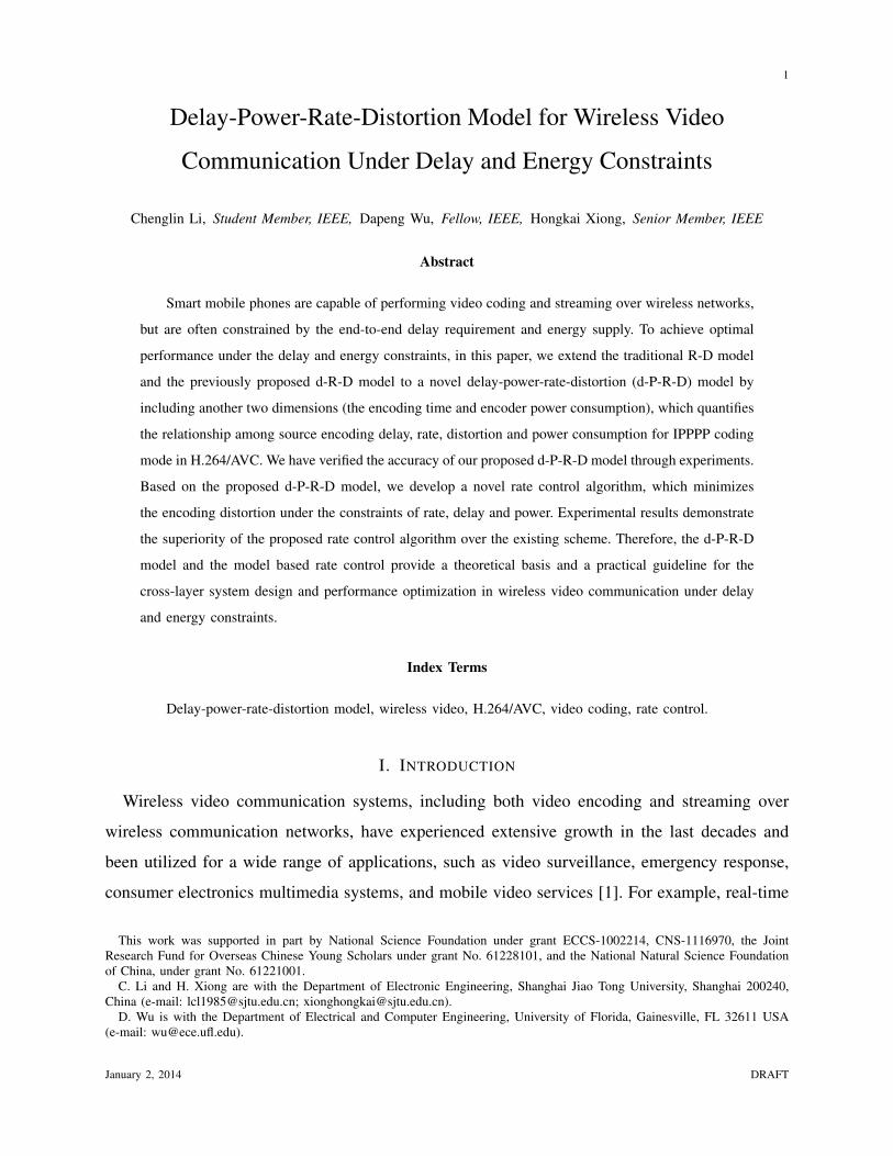
Fig. 1. End-to-end delay components of a video communication system.

entertainment traffic that comprises streaming both video and audio has already been making

up the majority of Internet traffic [2]. According to the Cisco visual networking index, mobile

video communication application will grow at a compound annual growth rate of 75 percent

between 2012 and 2017, the highest growth rate of any mobile application category [3]. Such

predictions lead to a natural but challenging question: how can we guarantee the quality of

service (QoS) metrics, such as end-to-end distortion, and end-to-end delay, for the wireless

video communication systems?

From the perspective of video encoding, if the video encoder is separately investigated without

consideration of its relationship with the subsequent transmission and the whole wireless video

communication system, transitional rate control (RC) plays an important role that affects the

overall R-D performance in the hybrid video codec design [4]. Based on the rate-distortion

optimization (RDO), rate control aims at minimizing the encoding distortion under a given

constraint on the encoding rate, by appropriate selections of several coding parameters, such as

quantization parameter (QP ) and macroblock (MB) mode. In this case, the encoding time and

power consumption are of little concern to the video encoder, since it can be assumed that there

is no limit on the encoding time and power consumption.

For the purpose of achieving the best end-to-end QoS performance, however, the entire

cross-layer wireless video communication system is expected to appropriately assign for the

video encoder both encoding time and encoding power according to the total end-to-end delay

constraint and a given maximum power supply. More specifically, for a practical real-time


3

wireless video communication system, the end-to-end delay can be broken up into several

delay components which, as illustrated in Fig. 1 respectively, are video encoding delay ∆Te,

encoder buffer delay ∆Teb, channel transmission delay ∆Tc, decoder buffer delay ∆Tdb, and

video decoding delay ∆Td [5], [6]. In [5] and [7], the video encoding time ∆Te and decoding

time ∆Td are both assumed to be constant. In fact, the video decoding time can be considered

as a part of the video encoding time, since the encoder has to decode the video sequence as

well. As illustrated in [1], [8], however, the video encoding time (delay) is determined by the

video encoding complexity, while the video encoding complexity would affect the source coding

incurred distortion and bit rate. Consequently, both the distortion and bit rate of the compressed

video that is transmitted over the channel is controlled by the video encoding time. On the

other hand, given an end-to-end delay constraint, if the encoding time is increased to achieve

better compression performance, the allowed queueing and buffering delay at encoding/decoding

buffers and channel delay for transmission will decrease accordingly, which in turn decreases

the delay constrained transmission throughput and thus increases the transmission distortion of

the compressed video. Generally, for a given end-to-end delay constraint, the overall system

performance depends on the allocation of end-to-end delay to different delay components. The

change of delay assignment in one component would cause changes of the delay budget in

other components, which would affect the overall system performance. Likewise, the mobile

video communication system is also power limited and needs to allocate its power supply to the

encoding/decoding modules and transmitting/receiving modules. For a given maximum power

supply, the change of the encoding power consumption would also impact on the power budget in

other modules and the overall system performance as well. Therefore, when the subsequent video

transmission is taken into account, video encoding delay and video encoding power consumption

become two new constraints which, as well, would affect the overall R-D performance of the

video communication systems and need to be considered in the rate control of the video encoder.

From the perspective of the cross-layer design of a wireless video communication system,

the delay and power consumption constraints on the video encoder are two-folded. On the

one hand, efficient video compression results in reduction of the bit rate of the video data,

leading to reduction in transmission power and/or transmission delay at the physical layer, or

reduction in the transmission rate and transmission error rate at data link layer. On the other

hand, efficient video compression often requires high computational complexity, leading to large


4

encoder power consumption and long encoding delay at the application layer. As implied by

these two conflicting aspects, there is a tradeoff among delay d, power consumption P , rate R,

and video distortion D for the design of the video encoder, which could be further applied to

control the QoS performance of the entire cross-layer wireless video communication system [9].

To find the optimal tradeoff solution, we need to develop an analytic framework to model the

delay-power-rate-distortion (d-P-R-D) behavior of the video encoder.

A. Related Work

Many rate control schemes have been proposed in literature to provide good video quality for

the encoded video while keeping its output bit rate within the bandwidth constraint for video

communication. Due to its efficiency, in the state-of-the-art video coding standard H.264/AVC,

JVT-G012 [10] is adopted by simply tuning QP to meet the target bit rate. In [11], the inter-

dependency between rate-distortion optimization and rate control is further improved by QP

estimation and update. Considering the initial QP for the first I-frame would influence the

rate control performance, a rate control scheme with adaptive QP initialization is proposed in

a content-aware manner [12]. In order to achieve a relatively steady visual quality, authors

in [13] develop a bit allocation scheme for both I-frame and P-frame based on the frame

complexity measurement and estimation model. Obviously, these schemes only focus on the

R-D performance of the video encoding system, while the other two dimensions, the encoding

time and power consumption are not taken into account.

In order to formulate the rate-distortion optimization problem, several bit rate and quantization

distortion models have been developed. Most existing work, e.g., [4] [14], derives the bit rate as

a function of video statistics and the quantization step size (or quantization parameter QP , there

is a one-to-one mapping between the quantization step size Q and the quantization parameter

QP [15], with Q increasing by 12.5% for each increment of 1 in QP ). Also, the quantization

distortion is derived as a function of the quantization step size and video statistics for a uniform

quantizer. In the rate-distortion model of [4], both the source rate and the source distortion for

a hybrid video coder with block based coding are derived as functions of the standard deviation

of the transformed residuals under the assumption of Laplacian distribution. By considering the

characteristics of variances of transformed residuals and compensating the mismatch between

the real histogram and the assumed Laplacian distribution, [16] improved both the bit rate


5

and distortion model where the Lagrangian based RDO is solved by the bi-section search. To

achieve the optimal selection of coding parameters, [4] converted the RDO to a Lagrangian

optimization problem and derived an accurate function between the single Lagrange multiplier

and quantization step size. However, none of them considers the analytic model of the encoding

time and power consumption, which makes the RDO not appropriate for the situation when

either encoding time or encoding power is constrained. Moreover, the bi-section search solver

would result in a relatively high computational complexity.

Many works have been done to analyze the rate-distortion-complexity of video encoders [1],

[6], [8], [17], [18], [19]. To derive the power-rate-distortion model for the video encoding system,

He et al. [1] summarized the encoding complexity of H.263 video encoder as three modules: mo-

tion estimation, PRE-coding (transform, quantization, inverse quantization and inverse transform),

and entropy coding. The relationship among the encoding complexity, rate, and distortion was

analyzed, and the power consumption level was adopted to represent the encoding complexity.

Unfortunately, this P-R-D model is dedicated to only H.263 video encoder. The model should

be evolved since H.264/AVC utilizes the tree structured motion compensation with seven inter-

modes, which causes the motion estimation consumes much more encoding complexity than

the other two modules. As a matter of fact, [1] also fails to consider the dimension of the

encoding time which is relevant to the encoding complexity. To tackle these issues, the delay-

rate-distortion (d-R-D) model of H.264/AVC video encoders was proposed and analyzed in [6],

[8] for both IPPPP and IBPBP coding modes. This d-R-D model depends on the quantization step

size and the standard deviation of transformed residuals in motion estimation (ME), which was

further fitted as functions of coding parameters in ME. However, this model did not consider and

analyze the encoding power consumption that is also closely related to the encoding complexity.

In addition, it neglects the critical impact of the quantization step size on both the standard

deviation of transformed residuals and the encoding delay component, which is demonstrated

based on extensive experiments.

B. Proposed Research

To our best knowledge, there has been no analytic framework for the d-P-R-D modeling of

the video encoding system, which is of great importance to analyze the effect of the video

encoding time and power consumption on the R-D performance of the video encoder. In this


6

work, we extend from the traditional R-D model [4], [16] and the d-R-D model previously

proposed in [6], [8], and accordingly develop an analytic framework to model, control and

optimize the delay-power-rate-distortion (d-P-R-D) behavior of the H.264/AVC video encoding

system. More specifically, our contributions in this paper are two-fold. First, four dimensions

(rate, distortion, delay and power) that jointly determine the performance of the H.264/AVC

video encoder are derived as functions of coding parameters (search range and number of

reference frames in motion estimation, and quantization step size), respectively. Here, without

loss of generality, the coding structure of the H.264/AVC encoder is chosen to be IPPPP coding

mode, which is also reasonable since as will be introduced, the motion estimation module

for inter-coded P-frames takes the major part of the entire encoding complexity. The model

accuracy has also been validated and compensated by considering the statistics of both the

current frame and the previous frame. Second, the proposed d-P-R-D model is applied to

formulate the source rate control problem as a d-P-R-D optimization problem with respect to the

search range and quantization step size. Compared with the existing work on source rate control

aiming at minimizing the video encoding distortion, we have introduced two more constraints

corresponding to the encoding time and the encoding power, in addition to the traditional

rate constraint. Furthermore, a practical algorithm based on both Karush-Kuhn-Tucker (KKT)

conditions and sequential quadratic programming (SQP) methods for the d-P-R-D optimization

based rate control problem is developed, which can produce both primal (search range and

quantization step size) and dual (Lagrange multipliers) solutions simultaneously and efficiently

in an iterative way. The proposed d-P-R-D model and model based rate control algorithm

provide a theoretical basis, as well as a practical guideline, for the cross-layer system design and

performance optimization in wireless video communication under delay and energy constraints.

By using the proposed d-P-R-D model, we can optimize the cross-layer performance (e.g.,

end-to-end distortion) by appropriately allocating the delay and power budget to components

within the wireless video communication system. It should be noted that, besides delay and

power limitation, bandwidth fluctuations and higher packet losses are also the challenges to be

addressed in wireless video communication systems. The main scope of this paper is how to

derive the d-P-R-D model and model based rate control problem for video encoders and propose

the model based source rate control algorithm. Therefore, at the encoder side, we only consider

the encoding delay which is a part of end-to-end delay, and encoding power which is a part


7

of the total system power consumption. The bandwidth fluctuations and high packet losses are

more related to the video packet transmission module of the wireless communication system,

and would be taken into account in our sequel paper that investigates the d-P-R-D performance

of the end-to-end wireless video communication systems comprising both video encoder and

video packet transmission part.

C. Paper Organization

The rest of the paper is organized as follows. In Section II, we derive the d-P-R-D source

coding model for H.264/AVC and verify the model accuracy based on experiments. In Section

III, we formulate a d-P-R-D optimization based source rate control problem, and accordingly

develop a practical algorithm based on KKT conditions and SQP methods to determine the

optimal selection of coding parameters. Section IV presents the experimental results, which

demonstrates the accuracy of the d-P-R-D model, the convergence behavior and performance of

the proposed algorithm. The concluding remarks and the future work are given in Section V.

II. D-P-R-D SOURCE CODING MODEL

According to the rate-distortion model proposed by Li [4] and Chen [16], both source rate and

source distortion for a hybrid video coder with block based coding, e.g., H.264/AVC encoder,

are based on the distribution of transformed residuals which is mainly determined by the motion

estimation (ME) accuracy and quantization distortion. More specifically, under the assumption

that the transformed residuals in ME follow Laplacian distribution [4] [20], the source rate and

distortion of an inter-coded P-frame in IPPPP coding mode can be derived as functions of the

standard deviation σ of the transformed residuals and the quantization step size Q (or quantization

parameter QP ). The extension to other distributions (e.g., Generalized Gaussian distribution [21]

and Cauchy distribution [22]) is also straightforward [16], since the transform coefficients are

supposed to be independent and identically distributed (i.i.d.).

To further analyze ME accuracy in H.264/AVC [23], the standard deviation σ of transformed

residuals depends on the following four coding parameters: 1) macroblock (MB) coding mode,

2) ME search range λ, 3) the number of reference frames θ [6], [8], and 4) quantization step

size Q. If the function relationship of σ(λ, θ,Q) can be established for H.264/AVC encoder, the


8

source rate and distortion will become functions of ME parameters λ, θ and quantization step

size Q.

On the other hand, both encoding time and encoding power are monotonously increasing

with encoding complexity. As will be justified in Sec. II-B, ME module is the most complexity

exhausting part within the entire encoding process and thus it is reasonable to approximate the

entire encoding complexity by ME complexity, which is measured by the number of sum of

absolute difference (SAD) operations for each MB partition (or subpartition): #SAD = (2λ +

1)2× θ [6], [8]. Therefore, by translating the specific coding behavior into encoding complexity,

both encoding time and power can be expressed as functions of ME parameters λ and θ. If

the encoding time is equivalently considered as video encoding delay, then the entire d-P-R-D

source coding model can be formulated.

Next, the closed form functions of rate, distortion, delay and power will be derived, respec-

tively.

A. Source Rate and Distortion Model

In order to develop the source rate and distortion model, the closed form function of σ(λ, θ,Q)

would be generated first. Due to the lack of any prior knowledge of the exact function form, a

basic means is to draw the relationship of σ versus λ, θ, and Q which can be fitted by a known

function form. To achieve it, the JM18.2 [24] coding engine is tested with the IPPPP coding mode

where the Bus (QCIF, 176× 144), Foreman (CIF, 352× 288), and Mobile (CIF, 352× 288) video

sequences are used to collect the statistics with a wide range of scene activity pattern, including

camera movement and large object motion (Bus), medium but complex motion (Foreman) and

motion with zooming effects (Mobile). For a fair evaluation, all MBs in the experiments would

select the same coding mode from the eight inter- modes except skip mode in order to exclude

the potential influence of MB coding mode in ME. Accordingly, these inter- modes are indicated

by index 1 to 7 as in JM configuration, (i.e., assigning index 1 to 16× 16 inter- mode, index 2

to 16× 8 inter- mode, etc.)

Since λ, θ and Q are independently tuned parameters in JM 18.2 configurations, we separately

evaluate their impacts on the average standard deviation σ of transformed residuals. For all the

seven inter- modes and the real mode selection where each MB chooses the best inter- mode

based on RDO, respectively, Fig. 2 illustrates the relationship between average standard deviation


9

σ of transformed residuals and search range λ, with fixed θ and Q. It can be seen from Figs.

2(a) and 2(c) that every curve obtained under one of the seven inter- modes or the real mode

selection resembles an exponential function with a constant vertical translation. In other words,

all the curves of seven inter- modes and the real mode selection have the similar functional

forms. In addition, as mode index increases from 1 to 7, the MB partition (or sub-partition)

size used to find the best match becomes smaller, which will lead to smaller predictive residuals

and thus smaller σ under the same search range λ. Accordingly, as presented in Fig. 2, the σ

vs. λ curve would slightly drop along σ direction as mode index increases. The curve of the

real mode selection is located in the middle of these curves, because each MB should select a

specific inter- mode out of the seven inter- modes. Comparing Figs. 2(a) and 2(c), it can also be

observed that more 16 × 16 inter- modes are assigned to Foreman sequence than Bus sequence

under the real mode selection. It can be indicated by the relative distance between the curve of

the real mode selection and the curve of the 16×16 inter- mode. Based on the analysis, similarly

as in [6], [8], we can use an exponential function with a constant vertical translation to fit the

curves in Figs. 2(a) and 2(c),

σ(λ) = a1e−b1λ + c1 (1)

where a1, b1 and c1 are fitting parameters. The corresponding fitting results are shown in Figs.

2(b) and 2(d).

It should be noted that in the training process of the source rate and distortion models, the

fast search algorithm is used in motion estimation to investigate the relationship between σ and

λ, θ, Q, for the sake of saving computational complexity. The peaks for certain λ values in

Figs. 2(a) and 2(c) are mainly because of the fast search algorithm. Specifically, with fast search

algorithm, the optimal motion vector that minimizes the SAD for each macroblock may not be

found, which would cause larger predictive residuals and thus larger σ than the optimal values

achieved by the exhaustive full search algorithm for certain λ values.

Likewise, the impact of number of reference frames θ on the average standard deviation σ

of transformed residuals is investigated in Fig. 3, at fixed λ and Q. The similar analysis and

observations can be drawn for the σ vs. θ curves as shown in Figs. 3(a) and 3(c). Hence, the σ


10

0 5 10 15 20 25 308

10

12

14

16

18

20

22

Search range λ

Ave

rage

σ

Bus

16 × 1616 × 88 × 168 × 88 × 44 × 84 × 4Real mode selection

(a)

0 5 10 15 20 25 30

10

12

14

16

18

20

22

24

Search range λ

Ave

rage

σ

Bus

16 × 16: σ=8.912e −0.5727λ+15.16

16 × 8: σ=8.036e −0.3895λ+14.12

8 × 16: σ=8.579e −0.4234λ+13.65

8 × 8: σ=8.846e −0.3822λ+12.25

8 × 4: σ=8.992e −0.3782λ+11.22

4 × 8: σ=9.44e −0.4321λ+11.26

4 × 4: σ=8.823e −0.3349λ+9.976

Real mode selection: σ=7.838e −0.403λ+12.95

(b)

0 5 10 15 20 25 303.5

4

4.5

5

5.5

6

6.5

Search range λ

Ave

rage

σ

Foreman


(c)

0 5 10 15 20 25 303.5

4

4.5

5

5.5

6

6.5

7

Search range λ

Ave

rage

σ

Foreman

16 × 16: σ=1.998e −0.9076λ+5.081

16 × 8: σ=2.242e −0.675λ+4.621

8 × 16: σ=1.798e −0.5949λ+4.701

8 × 8: σ=1.891e −0.6801λ+4.254

8 × 4: σ=2.353e −0.8394λ+4.047

4 × 8: σ=2.662e −0.718λ+4.091

4 × 4: σ=2.72e −0.7541λ+3.926

Real mode selection: σ=1.456e −0.5885λ+4.771

(d)

Fig. 2. Impact of search range on the average standard deviation of transformed residuals when θ = 4 and Q = 10, (a) Busvideo sequence, (b) the exponential fitting, and (c) Foreman video sequence , (d) the exponential fitting.

vs. θ curves can also be fitted by an exponential function plus a constant,

σ(θ) = a2e−b2θ + c2 (2)

where a2, b2 and c2 are fitting parameters. The corresponding fitting results are shown in Figs.

3(b) and 3(d). In comparison to the fitting results in Figs. 2(b) and 2(d), it can be seen that

since σ vs. θ curves are much more flatter than σ vs. λ curves, the decreasing rate of fitted

exponential functions in Fig. 3 is much smaller than that in Fig. 2. Therefore, search range λ is

a more effective parameter on the change of σ than the number of reference frames θ.

When λ and θ are fixed, the relationship between average standard deviation σ of transformed


11

1 2 3 4 5 6 7 8

10

12

14

16

18

20

22

Number of reference frames θ

Ave

rage

σ

Bus


(a)

1 2 3 4 5 6 7 8

10

12

14

16

18

20

22

24


Ave

rage

σ

Bus

16 × 16: σ=4.933e −1.127θ+14.94

16 × 8: σ=4.26e −0.7765θ+13.71

8 × 16: σ=5.011e −0.9025θ+13.41

8 × 8: σ=7.182e −0.9765θ+11.85

8 × 4: σ=3.974e −0.7742θ+10.79

4 × 8: σ=4.271e −0.7941θ+10.64

4 × 4: σ=3.164e −0.7944θ+9.579

Real mode selection: σ=5.314e −0.8723θ+12.59

(b)

1 2 3 4 5 6 7 83.5

4

4.5

5

5.5

6

6.5


Ave

rage

σ

Foreman


(c)

1 2 3 4 5 6 7 83.5

4

4.5

5

5.5

6

6.5

7


Ave

rage

σ

Foreman

16 × 16: σ=0.6149e −0.4736θ+4.955

16 × 8: σ=0.7497e −0.6115θ+4.524

8 × 16: σ=0.6359e −0.4323θ+4.571

8 × 8: σ=0.6442e −0.5226θ+4.143

8 × 4: σ=0.6055e −0.6059θ+3.947

4 × 8: σ=0.683e −0.5632θ+3.999

4 × 4: σ=0.6096e −0.6183θ+3.853

Real mode selection: σ=0.7543e −0.5008θ+4.647

(d)

Fig. 3. Impact of number of reference frames on the average standard deviation of transformed residuals when λ = 32 andQ = 10, (a) Bus video sequence, (b) the exponential fitting, and (c) Foreman video sequence, (d) the exponential fitting.

residuals and quantization step size Q is illustrated in Fig. 4. The σ vs. Q curves in Figs. 4(a)

and 4(c) indicate that they can be simply fitted by a linear function,

σ(Q) = a3Q+ b3 (3)

where a3 and b3 are fitting parameters. The corresponding linear fitting results are shown in Figs.

4(b) and 4(d). Similarly, quantization step size Q is a more effective parameter on the change

of σ than the number of reference frames θ.

In order to have a better understanding of Eqs. (1) - (3), we will discuss the impact of the

aforementioned four different factors on σ. Generally, an inter- mode with higher mode index


12

0 50 100 150 200 2505

10

15

20

25

30

Quantization step size Q

Ave

rage

σ

Bus

16 × 16

16 × 8

8 × 16

8 × 8

8 × 4

4 × 8

4 × 4Real mode selection

(a)

0 50 100 150 200 2500

5

10

15

20

25

30

35


Ave

rage

σ

Bus

16 × 16: σ=0.03436Q+14.91

16 × 8: σ=0.03907Q+13.76

8 × 16: σ=0.04013Q+13.39

8 × 8: σ=0.05481Q+11.73

8 × 4: σ=0.07107Q+10.63

4 × 8: σ=0.07473Q+10.4

4 × 4: σ=0.1053Q+9.112

Real mode selection: σ=0.06212Q+12.35

(b)

0 50 100 150 200 2502

4

6

8

10

12

14

16

18


Ave

rage

σ

Foreman

16 × 16

16 × 8

8 × 16

8 × 8

8 × 4

4 × 8

4 × 4Real mode selection

(c)

0 50 100 150 200 250

5

10

15

20

25


Ave

rage

σ

Foreman

16 × 16: σ=0.02307Q+4.928

16 × 8: σ=0.02679Q+4.419

8 × 16: σ=0.02581Q+4.622

8 × 8: σ=0.0338Q+3.917

8 × 4: σ=0.04339Q+3.569

4 × 8: σ=0.0429Q+3.664

4 × 4: σ=0.05829Q+3.579

Real mode selection: σ=0.04434Q+4.383

(d)

Fig. 4. Impact of quantization step size on the average standard deviation of transformed residuals when λ = 32 and θ = 4,(a) Bus video sequence,(b) the linear fitting, and (c) Foreman video sequence, (d) the linear fitting.

(i.e., with smaller size of MB partitions) will lead to better prediction, and thus the standard

deviation σ of transformed residuals tends to be smaller. For the real mode selection, since MB

can choose a best mode out of all the seven inter- modes, the value of σ is bounded within

mode 1 and mode 7. On the other hand, either a larger search range λ or a larger number of

reference frames θ will result in a bigger 3-D search cube in ME and thus a better prediction,

which would also lead to a smaller σ. The last factor, quantization step size Q, would affect

the distortion of the reference frames. Generally, the distortion of the reference frames will be

increased by the selection of larger Q, which tends to result in larger σ.

From Figs. 2-4, it can also be seen that θ has little contribution to the change of σ compared


13

5

10

15

50100

150200

10

20

30

40

50

Search range λ

Bus


Ave

rage

σσ=10.99e−0.662λ+14.2+0.07305Qσ vs. λ, Q

(a)

5

10

15

50100

150200

0

5

10

15

20

25

30

Search range λ

Foreman


Ave

rage

σ

σ=3.378e−0.4997λ+4.299+0.05877Qσ vs. λ, Q

(b)

510

15

50100

150200

15

20

25

30

Search range λ

Mobile


Ave

rage

σ

σ=1.22e−0.3809λ+15.22+0.03676Qσ vs. λ, Q

(c)

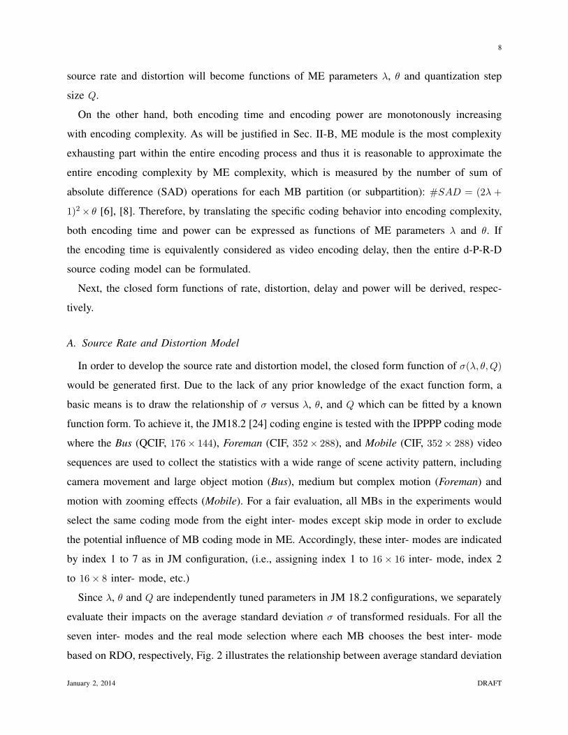
Fig. 5. Two dimensional fitting of the average standard deviation of transformed residuals vs. search range and quantizationstep size, (a) Bus video sequence with θ = 1, R-square=0.965 and RMSE=0.845 (b) Foreman video sequence with θ = 1,R-square=0.936 and RMSE=0.884, (c) Mobile video sequence with θ = 1, R-square=0.884 and RMSE=0.763.

with the other two parameters. For example, for the same mode, the changing rate of σ vs. θ is

much smaller than that of σ vs. λ and σ vs. Q. In the real mode selection, we could investigate

the function σ(λ,Q) for given θ = θ0 which approximates the function σ(λ, θ,Q), for the sake of

simplicity. Another motivation is that by fixing the value of θ, the computational complexity for

fitting the standard deviation function σ(λ, θ,Q) would be decreased. Fig. 5 illustrates the two

dimensional fitting results of function σ(λ,Q) with θ fixed at 1. Considering both the exponential

relationship with λ and linear relationship with Q, the fitted two dimensional function of σ can

be represented in the form of

σ(λ,Q) = ae−bλ + c+ dQ ≈ σ(λ, θ,Q) (4)


14

where a, b, c and d are fitting parameters. Based on the fitting results, we have obtained the

closed form function of σ(λ,Q), which is an approximation of σ(λ, θ,Q). To better assess the

fitting performance, both R-square and RMSE (root mean square error) are used as the metrics

to measure the degree of data variation from the proposed model (4), as shown in Fig. 5. It

should be noted that although the fitting accuracy could be improved by using other high-order

or complex function forms, the computational complexity would also be increased. In accordance

with wireless video communication systems, and for the sake of simplicity, we only apply the

simple function form as expressed by Eq. (4) which could also achieve overall acceptable fitting

performance.

For i.i.d. zero-mean Laplacian source under the uniform quantizer, the closed form functions

of entropy of quantized transform coefficients and quantization distortion have been provided

in [16]. Furthermore, the entropy of quantized transformed residual can approximate the source

rate model when no effect by side information such as macroblock type and motion information

[4]. Hence, the closed form of source rate model is given by:

R(Λ, Q) = H(Λ, Q) = −P0 log2 P0 + (1− P0)

[ΛQ log2 e

1− e−ΛQ− log2(1− e−ΛQ)− ΛQγ log2 e+ 1

](5)

where Λ =√2/σ is the Laplace parameter that is one-to-one mapping of σ; γQ represents

the rounding offset when γ is a parameter between (0, 1), such as 1/6 for H.264/AVC inter-

frame coding [4]; P0 = 1− e−ΛQ(1−γ) is the probability of quantized transform coefficient being

zero. Since the source distortion is only caused by quantization error, the corresponding source

distortion model is expressed as:

D(Λ, Q) =ΛQeγΛQ(2 + ΛQ− 2γΛQ) + 2− 2eΛQ

Λ2(1− eΛQ)(6)

The derivation process and proof of Eqs. (5) and (6) are given in Appendix A. Integrating Eq.

(4) and Λ =√2/σ into Eqs. (5) and (6), both source rate and distortion can be further expressed

as functions of λ and Q, i.e., R(λ,Q) and D(λ,Q).


15

B. Encoding Time and Power Model

As introduced in [1], the encoding complexity comprises of three segments: motion estimation,

PRE-coding (transform, quantization, inverse quantization and inverse transform), and entropy

coding. Theoretically, the entire encoding time is the sum of individual duration of each of

the three segments. In order to achieve higher compression efficiency, H.264/AVC utilizes tree

structured motion compensation with seven inter- modes, which causes ME as the most time

consuming part within all the three segments of the encoder. Likewise, Fig. 6 illustrates the

ratio of motion estimation time to the entire encoding time for the Bus (QCIF) and Foreman

(CIF) sequences, with regard to search range and number of reference frames. Here, for a specific

sequence, the motion estimation time ratio is obtained by dividing the average motion estimation

time by the average entire encoding time for a P-frame. It can be seen from Figs. 6(a) and 6(b)

that ME takes majority of the entire encoding time, e.g. more than 90% when λ greater than

5 and within all the range of θ. Furthermore, the ratio grows and approaches to 1 with the

increment of search range and number of reference frames. Thus, as demonstrated in [6], [8], it

is reasonable to approximate the entire encoding time by the motion estimation time for IPPPP

coding mode. It is worth mentioning that the ME time ratio throughout this paper is attained by

exhaustive full search, which can guarantee achieving the optimal motion vector and minimum

predictive residuals.

Technically, the motion estimation time of an inter-coded P frame can be derived as the total

number of CPU clock cycles consumed by its SAD operation divided by the number of clock

cycles per second. Namely, the encoding time for an inter-coded P frame is approximated by

the motion estimation time as

d(λ, θ) ≈ MET (λ, θ) =N(2λ+ 1)2θ · c0

fCLK(7)

where N is the number of MBs in a frame; (2λ+1)2θ is the total number of SAD operations in

a 3-D search cube for each MB; c0 is the number of clock cycles of one SAD operation over

a given CPU; fCLK is the clock frequency of the CPU. Through the dynamic voltage scaling

model to control power consumption of a microprocessor [25] [26], fCLK can be further related


16

0 5 10 15 20 25 300.4

0.5

0.6

0.7

0.8

0.9

1

Search range λ (θ=4, Q=10)

ME

tim

e ra

tio

Bus

(a)

1 2 3 4 5 6 7 80.9

0.91

0.92

0.93

0.94

0.95

0.96

0.97

0.98

0.99

1

Number of reference frames θ (λ=16, Q=10)

ME

tim

e ra

tio

Bus

(b)

0 5 10 15 20 25 300.2

0.3

0.4

0.5

0.6

0.7

0.8

0.9

1


ME

tim

e ra

tio

Foreman

(c)

1 2 3 4 5 6 7 80.75

0.8

0.85

0.9

0.95

1


ME

tim

e ra

tio

Foreman

(d)

Fig. 6. Impact of search range and number of reference frames on the motion estimation time ratio, (a) search range and (b)number of reference frames of Bus video sequence, and (c) search range and (d) number of reference frames of Foreman videosequence.

to the CPU power consumption:

P = k · f3CLK (8)

where k is a constant in the dynamic voltage scaling model and determined by both the supply

voltage and the effective switched capacitance of the circuits [27].

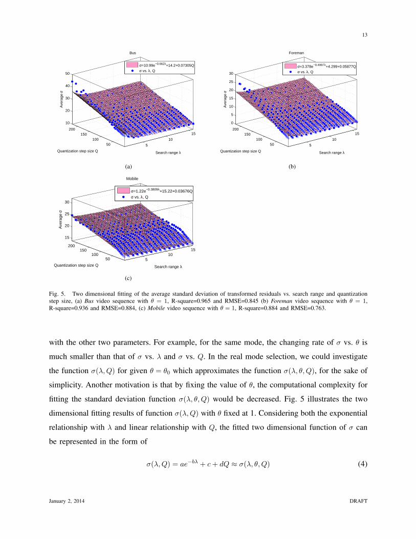
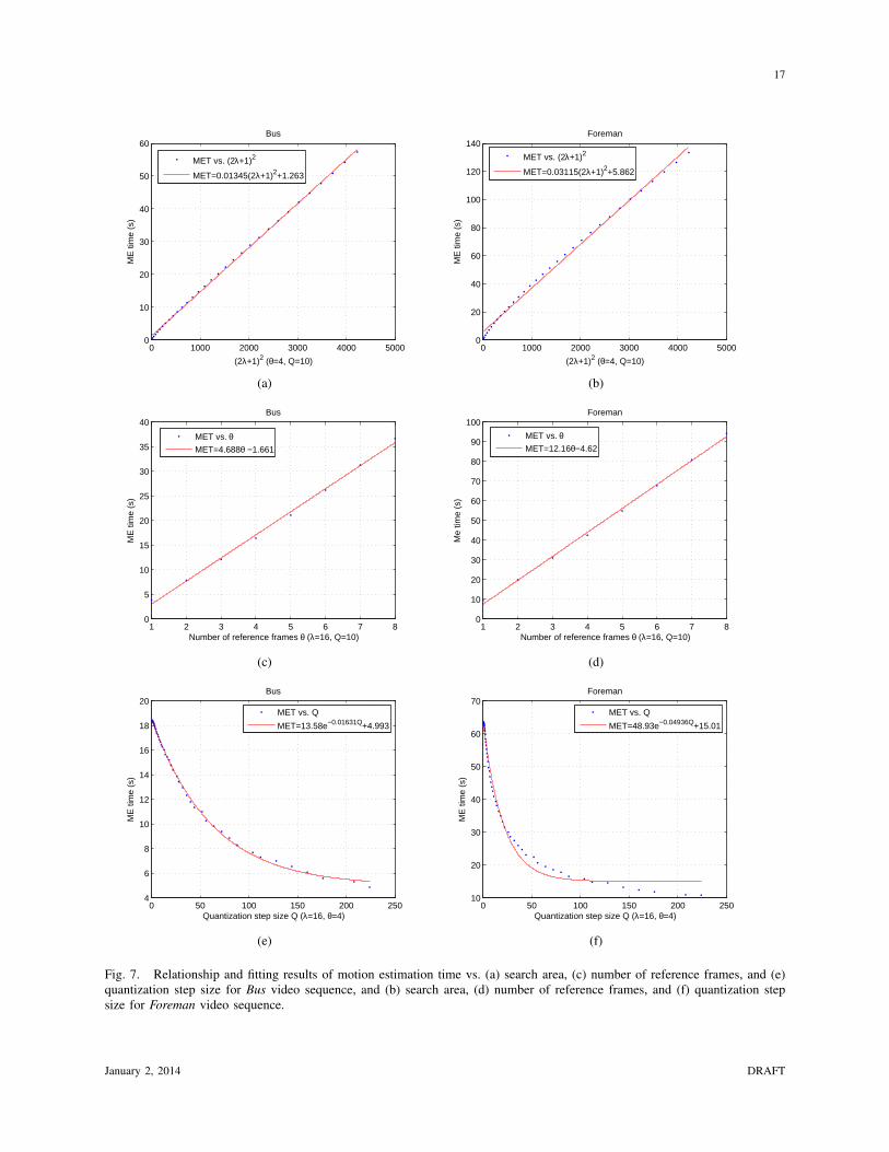
To justify the theoretical encoding time model in Eq. (7), Fig. 7 is provided to further

investigate the relationship between the motion estimation time (MET) and ME parameters λ,

θ and quantization step size Q. It can be seen from Figs. 7(a) and 7(b) that MET can be fitted

by a linear function of either search area (2λ + 1)2 or the number of pixels ever searched in a


17

0 1000 2000 3000 4000 50000

10

20

30

40

50

60

(2λ+1)2 (θ=4, Q=10)

ME

tim

e (s

)Bus

MET vs. (2λ+1)2

MET=0.01345(2λ+1)2+1.263

(a)

0 1000 2000 3000 4000 50000

20

40

60

80

100

120

140

(2λ+1)2 (θ=4, Q=10)

ME

tim

e (s

)

Foreman

MET vs. (2λ+1)2

MET=0.03115(2λ+1)2+5.862

(b)

1 2 3 4 5 6 7 80

5

10

15

20

25

30

35

40


ME

tim

e (s

)

Bus

MET vs. θMET=4.688θ −1.661

(c)

1 2 3 4 5 6 7 80

10

20

30

40

50

60

70

80

90

100


Me

time

(s)

Foreman

MET vs. θMET=12.16θ−4.62

(d)

0 50 100 150 200 2504

6

8

10

12

14

16

18

20

Quantization step size Q (λ=16, θ=4)

ME

tim

e (s

)

Bus

MET vs. Q

MET=13.58e−0.01631Q+4.993

(e)

0 50 100 150 200 25010

20

30

40

50

60

70


ME

tim

e (s

)

Foreman

MET vs. Q

MET=48.93e−0.04936Q+15.01

(f)

Fig. 7. Relationship and fitting results of motion estimation time vs. (a) search area, (c) number of reference frames, and (e)quantization step size for Bus video sequence, and (b) search area, (d) number of reference frames, and (f) quantization stepsize for Foreman video sequence.


18

reference frame. Similarly, Figs. 7(c) and 7(d) indicate that MET can also be fitted by a linear

function of number of reference frames θ. In accordance with Eq. (7), the linear relationship

between MET and (2λ+1)2 or θ is obvious, since (2λ+1)2 ·θ would form a 3-D search cube for

a MB in ME and represent the total number of SAD operations per MB. In Figs. 7(e) and 7(f),

MET is illustrated to be dependent on quantization step size Q too. The relationship can be well

fitted by an exponential function with a constant translation along the MET axis. Specifically, the

higher the quantization step size is, the more likely a MB would satisfy the skip mode condition

and thus the more MBs would end up with skip mode as the real coding mode, which can

lower the encoding complexity. The higher the quantization step size is, the fewer number of

SAD operations for each MB is involved, and the lower complexity to encode the inter-frame.

Hence, Eq. (7) is modified to reflect such dependency between the motion estimation time and

the quantization step size:

d(λ, θ,Q) ≈ MET (λ, θ,Q) =N(2λ+ 1)2θ · α(Q) · c0

fCLK(9)

where α(Q) denotes the ratio of the actual number of SAD operations in the JM codec to the

theoretical total number of SAD operations, and thus N(2λ + 1)2θ · α(Q) represents the actual

number of SAD operations of a frame.

Fig. 8 illustrates the relationship of MET vs. search area and quantization step size, with

number of reference frames fixed at 1, namely, the functional form of d(λ, θ,Q|θ = 1). Comparing

the two dimensional fitting results with Eq. (9), it can be observed thatN · α(Q) · c0

fCLK= 0.003612 ·

(0.7422e−0.01113Q + 0.212), where N = 99 for QCIF video sequence. The correctness of Eq. (9)

can also be validated by the results in Fig. 7.

C. Model Accuracy Verification

1) Source Rate and Distortion: According to [28], the transform coefficients in a video

encoder are not i.i.d.. As described in [16], the 16 coefficients in a 4× 4 integer transform show

a decreasing variance in the zigzag scan order. To improve the model accuracy of source rate

and distortion, the coefficients should be modeled by random variables with different variances.

The joint entropy and overall quantization distortion for the 16 coefficients can be applied to the

source rate and distortion models. Specifically, suppose (x, y), x, y ∈ {0, 1, 2, 3} is the position


19

200400

600800

1000

50100

150200

0

1

2

3

4

5

(2λ+1)2

Bus


ME

tim

e (s

)MET=0.003612⋅(2λ+1)2⋅(0.7422e−0.01113Q+0.212)

MET vs. (2λ+1)2, Q

(a)

200400

600800

1000

50100

150200

0

5

10

15

20

(2λ+1)2

Foreman


ME

tim

e (s

)

MET=0.05953⋅(2λ+1)2⋅(0.1887e−0.5654Q+0.05653)

MET vs. (2λ+1)2, Q

(b)

Fig. 8. Two dimensional fitting of motion estimation time vs. search area and quantization step size with θ = 1, (a) Bus videosequence, and (b) Foreman video sequence.

of a specific coefficient in the two-dimensional transform domain of the 4× 4 integer transform,

the variance σ2(x,y) is derived by the average variance σ2 of all positions.

σ2(x,y) = 2−(x+y) · σ2

(0,0) = 2−(x+y) · 1024225

σ2 (10)

Therefore, the source rate and distortion model can be improved by:

R(Λ, Q) = H(Λ, Q) =1

16

3∑x=0

3∑y=0

H(Λ, Q)(x,y) (11)

D(Λ, Q) =1

16

3∑x=0

3∑y=0

D(Λ, Q)(x,y) (12)

where Λ =√2/σ is the Laplace parameter as defined in Eq. (5), H(Λ, Q)(x,y) and D(Λ, Q)(x,y)

are the entropy and distortion associated with coefficient in position (x, y), respectively.

Considering the Laplacian distribution representing the residual probability distribution may

deviate significantly from the residual histogram, in addition, the mismatch would be compen-

sated by the statistics from the previous frame [16], [6],:

Rkt =

Rk−1t Rk

l

Rk−1l

(13)


20

0 2 4 6 8 10 12 14 161.7

1.8

1.9

2

2.1

2.2

2.3

2.4

2.5

2.6

2.7Bus


Bit

rate

(bp

p)

True bppEstimated bpp by Eq. (5)Improved bpp by Eq. (11)Improved bpp by Eqs. (11) and (13)

(a)

0 2 4 6 8 10 12 14 168

10

12

14

16

18

20

22Bus


Dis

tort

ion

(MS

E)

True MSEEstimated MSE by Eq. (6)Improved MSE by Eq. (12)Improved MSE by Eq. (12) and (14)

(b)

0 10 20 30 40 50 600

0.5

1

1.5

2

2.5

3Bus


Bit

rate

(bp

p)


(c)

0 10 20 30 40 50 600

50

100

150

200

250Bus


Dis

tort

ion

(MS

E)


(d)

Fig. 9. Compensation results of (a) bit rate and (b) MSE vs. search range for Bus video sequence, and (c) bit rate and (d)MSE vs. quantization step size for Bus sequence.

Dkt =

Dk−1t Dk

l

Dk−1l

(14)

where superscripts k − 1 and k denote the frame index of two consecutive frames, subscripts

l and t denote the estimated value under Laplacian distribution assumption and the true value,

respectively.

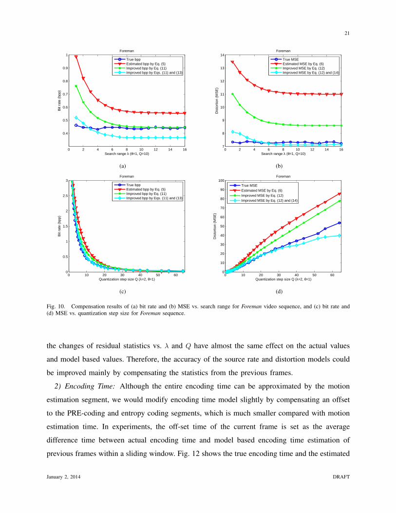
In Figs. 9-11, the accuracy of the proposed source rate model Eq. (5) and distortion model Eq.

(6) is evaluated in comparison to the actual bit per pixel (bpp) and MSE measures. In addition,

the compensated model estimate of source rate and distortion on Eqs. (11) and (12), as well as

the improvement on Eqs. (13) and (14), are illustrated. According to [16], in a video sequence,


21

0 2 4 6 8 10 12 14 16

0.4

0.5

0.6

0.7

0.8

0.9

1Foreman


Bit

rate

(bp

p)


(a)

0 2 4 6 8 10 12 14 167

8

9

10

11

12

13

14Foreman


Dis

tort

ion

(MS

E)


(b)

0 10 20 30 40 50 600

0.5

1

1.5

2

2.5

3Foreman


Bit

rate

(bp

p)


(c)

0 10 20 30 40 50 600

10

20

30

40

50

60

70

80

90

100Foreman


Dis

tort

ion

(MS

E)


(d)

Fig. 10. Compensation results of (a) bit rate and (b) MSE vs. search range for Foreman video sequence, and (c) bit rate and(d) MSE vs. quantization step size for Foreman sequence.

the changes of residual statistics vs. λ and Q have almost the same effect on the actual values

and model based values. Therefore, the accuracy of the source rate and distortion models could

be improved mainly by compensating the statistics from the previous frames.

2) Encoding Time: Although the entire encoding time can be approximated by the motion

estimation segment, we would modify encoding time model slightly by compensating an offset

to the PRE-coding and entropy coding segments, which is much smaller compared with motion

estimation time. In experiments, the off-set time of the current frame is set as the average

difference time between actual encoding time and model based encoding time estimation of

previous frames within a sliding window. Fig. 12 shows the true encoding time and the estimated


22

0 2 4 6 8 10 12 14 161.8

1.9

2

2.1

2.2

2.3

2.4

2.5Mobile


Bit

rate

(bp

p)


(a)

0 2 4 6 8 10 12 14 166

8

10

12

14

16

18

20

22Mobile


Dis

tort

ion

(MS

E)


(b)

0 10 20 30 40 50 600

0.5

1

1.5

2

2.5

3Mobile


Bit

rate

(bp

p)


(c)

0 10 20 30 40 50 600

50

100

150

200

250Mobile


Dis

tort

ion

(MS

E)


(d)

Fig. 11. Compensation results of (a) bit rate and (b) MSE vs. search range for Bus video sequence, and (c) bit rate and (d)MSE vs. quantization step size for Mobile sequence.

encoding time, which can be seen that the difference between the encoding time model Eq. (9)

and its true value is relatively small. As the encoding time increases, the difference would become

less significant.

III. D-P-R-D OPTIMIZATION BASED SOURCE RATE CONTROL AND ALGORITHM DESIGN

FOR IPPPP CODING MODE

In this section, we apply the proposed models in Sec. II to formulate the source rate control

problem as a d-P-R-D optimization with respect to search range λ and quantization step size Q,

and accordingly design a practical rate control algorithm.


23

0 200 400 600 800 1000 12000

0.5

1

1.5

2

2.5

3

3.5

4

4.5Bus

(2λ+1)2 (θ=1,Q=10)

Enc

odin

g tim

e (s

)

True valueEstimated by Eq. (9)Compensated by an offset of 0.5 s

(a)

0 50 100 150 200 2501

1.5

2

2.5

3

3.5

4

4.5

5

5.5Bus

Quantization step size Q (λ=16,θ=1)

Enc

odin

g tim

e (s

)

True valueEstimated by Eq. (9)Compensated by an offset of 0.5 s

(b)

0 200 400 600 800 1000 12000

2

4

6

8

10

12

14Foreman

(2λ+1)2 (θ=1,Q=10)

Enc

odin

g tim

e (s

)

True valueEstimated by Eq. (9)Compensated by an offset of 2 s

(c)

0 50 100 150 200 2502

4

6

8

10

12

14

16

18

20Foreman


Enc

odin

g tim

e (s

)


(d)

0 200 400 600 800 1000 12000

2

4

6

8

10

12

14

16

18Mobile

(2λ+1)2 (θ=1,Q=10)

Enc

odin

g tim

e (s

)


(e)

0 50 100 150 200 2504

6

8

10

12

14

16

18

20

22Mobile


Enc

odin

g tim

e (s

)


(f)

Fig. 12. Compensation results of encoding time vs. (a) search area and (b) quantization step size for Bus video sequence, and(c) search area and (d) quantization step size for Foreman video sequence, and (e) search area and (f) quantization step size forMobile video sequence.


24

A. d-P-R-D Optimization Based Source Rate Control

In the previous section, we have derived the analytical models of rate, distortion, delay and

power, as functions of three parameters, search range λ, number of reference frames θ, and

quantization step size Q, respectively. As discussed in Sec. II-A, however, θ is a less effective

parameter on the change of σ than the other two parameters. To this end, we keep the value of

θ fixed and choose λ and Q as the tuning parameters, and thus the d-P-R-D optimization based

source rate control problem can be formulated as

min D(λ,Q) (15a)

s.t. R(λ,Q) ≤ Rmax (15b)

d(λ,Q) ≤ dmax (15c)

P ≤ Pmax (15d)

Compared with the existing works on source rate control problems, the optimization problem

Eq. (15) is constrained by two more conditions of the encoding time and encoding power, in

addition to the rate. Ideally, an efficient video encoder is expected to encode a raw video sequence

into a bit stream with minimum distortion, rate, encoding delay and encoding power. From the

analysis of the proposed d-P-R-D models in Sec. II, it can be seen that a larger search range λ as

well as a smaller quantization step size Q is required to achieve the objective of minimizing the

distortion D(λ,Q). On the other hand, however, the decrement of Q will cause the rate R(λ,Q)

to increase, and the encoding delay d(λ,Q) will also become greater with either λ increasing or

Q decreasing. Furthermore, for a coding parameter pair (λ,Q), the encoding delay d(λ,Q) can

be further reduced by increasing the encoding power P , while the distortion and rate are still

kept at the same level. Therefore, it is infeasible for a video encoder to simultaneously achieve

the goals of minimizing distortion, rate, encoding delay and encoding power. Accordingly, the

d-P-R-D optimization based source rate control problem Eq. (15) is to find the Pareto optimal

tradeoff among the four optimization criteria. As a matter of fact, the target of such optimization

is to minimize the distortion D(λ,Q) for given rate Rmax, given encoding delay dmax and given

encoding power Pmax, by appropriate selections of coding parameter pair (λ,Q).

Depending on the estimation accuracy of the d-P-R-D models, the source rate control problem


25

Eq. (15) can be applied to a desired coding unit, e.g. a sequence, a group of pictures (GOP),

a frame, or a macroblock. For example, if the d-P-R-D model is applied to a stream, Eq. (15)

can be regarded to solve the sequence level rate control problem. If it is applied to a frame, Eq.

(15) can behave as a frame level rate control. Without loss of generality, a sequence level rate

control problem will be imposed on Eq. (15) with a practical solution.

B. Algorithm Design

Considering both Eqs. (8) and (9), for the coding parameter pair (λ,Q), the minimum encoding

delay would be achieved with the maximal power Pmax. In other words, the feasible set of coding

parameters (λ,Q) constrained by a given maximum encoding delay would become the largest if

and only if the encoding power reaches the maximum. According to Proposition 1, the power

constraint (15d) in (15) is therefore an active constraint at the optimal coding parameter pair

(λ∗, Q∗), and the source rate control problem Eq. (15) can be transformed to an equivalent

problem Eq. (16).

Proposition 1. Problem (15) is equivalent to the following optimization problem:

min D(λ,Q) (16a)

s.t. R(λ,Q) ≤ Rmax (16b)

d(λ,Q) ≤ dmax (16c)

P = Pmax (16d)

Proof: Please refer to [29].

Either the Lagrange multiplier method [30] [31] [32] or the dynamic programming approach

[33] can solve Eq. (16). The former is preferred throughout this paper since it can be implemented

independently in each coding unit. In comparison, the dynamic programming approach requires

a tree representing all possible solutions to grow over multiple coding units. The computational

complexity would grow exponentially with the number of coding units, which is not affordable

for practical applications. With the Lagrange multiplier method, Eq. (16) can be converted to an

unconstrained problem Eq. (17):

min L(λ,Q, µ, η) = D(λ,Q) + µ · [R(λ,Q)−Rmax] + η · [d(λ,Q)− dmax] (17)


26

where µ ≥ 0 and η ≥ 0 are Lagrange multipliers associated with two inequality constraints, and

the equality constraint P = Pmax can be integrated to d(λ,Q) as:

d(λ,Q) =N(2λ+ 1)2θ · α(Q) · c0

3√

k−1Pmax

(18)

Based on the theorem in [30], we have the following theorem that relates the solution to the

unconstrained problem Eq. (17) to the solution to the constrained problem Eq. (16).

Theorem 1. For any µ ≥ 0, η ≥ 0, the solution (λ∗, Q∗) to the unconstrained problem Eq. (17)

is also the solution to the constrained problem Eq. (16) with the constraints R(λ,Q) ≤ R(λ∗, Q∗)

and d(λ,Q) ≤ d(λ∗, Q∗).

Proof: Please refer to [32].

It should be noted that although Theorem 1 does not guarantee any solution to the constrained

problem Eq. (16), it indicates that for any nonnegative µ and η, there is a corresponding

constrained problem whose solution is identical to that of the unconstrained problem. Therefore,

as µ and η are swept over the range [0,+∞], if there exists a specific pair of µ∗ and η∗ which

makes R(λ∗, Q∗) and d(λ∗, Q∗) happen to be equal to Rmax and dmax, then (λ∗, Q∗) is the desired

solution to the constrained problem Eq. (16).

To estimate the corresponding µ∗ and η∗ in practice, the bi-section search method [16] [32] is

commonly used for iterations to acquire the best Lagrange multiplier. However, two disadvantages

have prevented such method from being suitably applied to the unconstrained problem Eq. (17).

First, the bi-section search method would perform worse or even fail to get the solution when

extended to two dimensional search scenario. For example, if we simultaneously bisect the

intervals for µ and η and then select a subinterval for each of these two Lagrange multipliers

based on their own criteria, respectively, the best solution µ∗ and η∗ might be excluded by

such independent bisections. Therefore, in order to get the best solution, in many cases we

have to implement an exhausting search over two dimensions, which is very time consuming.

Second, even if the bi-section search can suitably work for searching two Lagrange multipliers

simultaneously, we still need to update the Lagrange multipliers in each iteration, and then solve

the corresponding unconstrained problem Eq. (17) to get the solution. It means the update of

primal and dual variables are not synchronous and may cause high computational complexity.


27

Another analytical way to determine the best Lagrange multiplier is the model-based method [4]

[31], which focuses on rate-distortion optimization and accordingly derives an accurate function

between the single Lagrange multiplier and Q. Without consideration of the encoding time and

power, however, the derived function is no longer accurate and thus cannot be directly applied

to the d-P-R-D optimization.

In the following, we propose a practical algorithm for the d-P-R-D optimization based source

rate control problem Eq. (16) on the basis of KKT conditions and sequential quadratic pro-

gramming (SQP) methods, which can produce both primal (λ∗ and Q∗) and dual (Lagrange

multipliers µ∗ and η∗) solutions simultaneously in an iterative way. To solve the first-order

necessary conditions of optimality for problem Eq. (16), the SQP methods [34] [35] can be used

to construct a quadratic programming subproblem at a given approximate solution, and then

to employ the solution to this subproblem to construct a better approximation. This process is

iterated to create a sequence of approximations that is expected to converge to the optimal solution

(λ∗, Q∗, µ∗, η∗). Specifically, given an iterate (λk, Qk, µk, ηk), a new iterate (λk+1, Qk+1, µk+1, ηk+1)

can be obtained by solving a quadratic programming (QP) minimization subproblem given by:

minδk

∂D(λk, Qk)

∂λ· δkλ +

∂D(λk, Qk)

∂Q· δkQ +

1

2δk

T · ∇2L(λk, Qk, µk, ηk) · δk (19a)

s.t.∂R(λk, Qk)

∂λ· δkλ +

∂R(λk, Qk)

∂Q· δkQ +R(λk, Qk) = Rmax (19b)

∂d(λk, Qk)

∂λ· δkλ +

∂d(λk, Qk)

∂Q· δkQ + d(λk, Qk) = dmax (19c)

where the derivative operators ∇2 is used to refer to the second-order Hessian matrix with

respect to primal variables λ and Q, and δk = (δkλ, δkQ)

T = (λk+1 − λk, Qk+1 −Qk)T is the vector

representing the update directions of primal variables. For details about the derivation of Eq.

(19), please refer to Appendix B.

The aforementioned SQP algorithm, though can be used to appropriately solve Eq. (16),

suffers from two deficiencies similar to the Newton’s method. First, it requires at each iteration

the calculation of second-order Hessian matrix ∇2L(λk, Qk, µk, ηk), which could be a costly

computational burden and in addition might not be positive definite. To address this issue, we

can use the quasi-Newton method instead to construct an approximate Hessian matrix Bk by

which ∇2L(λk, Qk, µk, ηk) is replaced in Eq. (19). In practice, such an approximation Bk can be


28

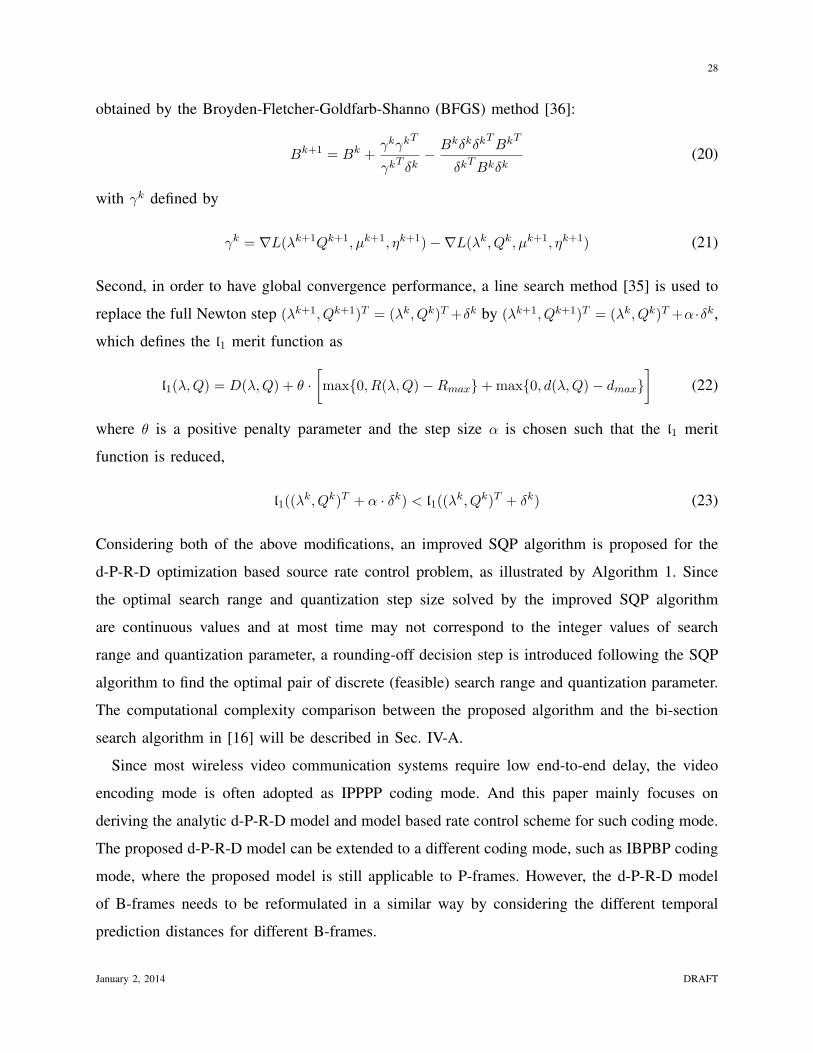
obtained by the Broyden-Fletcher-Goldfarb-Shanno (BFGS) method [36]:

Bk+1 = Bk +γkγk

T

γkTδk

− BkδkδkTBkT

δkTBkδk

(20)

with γk defined by

γk = ∇L(λk+1Qk+1, µk+1, ηk+1)−∇L(λk, Qk, µk+1, ηk+1) (21)

Second, in order to have global convergence performance, a line search method [35] is used to

replace the full Newton step (λk+1, Qk+1)T = (λk, Qk)T +δk by (λk+1, Qk+1)T = (λk, Qk)T +α ·δk,

which defines the l1 merit function as

l1(λ,Q) = D(λ,Q) + θ ·[max{0, R(λ,Q)−Rmax}+max{0, d(λ,Q)− dmax}

](22)

where θ is a positive penalty parameter and the step size α is chosen such that the l1 merit

function is reduced,

l1((λk, Qk)T + α · δk) < l1((λ

k, Qk)T + δk) (23)

Considering both of the above modifications, an improved SQP algorithm is proposed for the

d-P-R-D optimization based source rate control problem, as illustrated by Algorithm 1. Since

the optimal search range and quantization step size solved by the improved SQP algorithm

are continuous values and at most time may not correspond to the integer values of search

range and quantization parameter, a rounding-off decision step is introduced following the SQP

algorithm to find the optimal pair of discrete (feasible) search range and quantization parameter.

The computational complexity comparison between the proposed algorithm and the bi-section

search algorithm in [16] will be described in Sec. IV-A.

Since most wireless video communication systems require low end-to-end delay, the video

encoding mode is often adopted as IPPPP coding mode. And this paper mainly focuses on

deriving the analytic d-P-R-D model and model based rate control scheme for such coding mode.

The proposed d-P-R-D model can be extended to a different coding mode, such as IBPBP coding

mode, where the proposed model is still applicable to P-frames. However, the d-P-R-D model

of B-frames needs to be reformulated in a similar way by considering the different temporal

prediction distances for different B-frames.


29

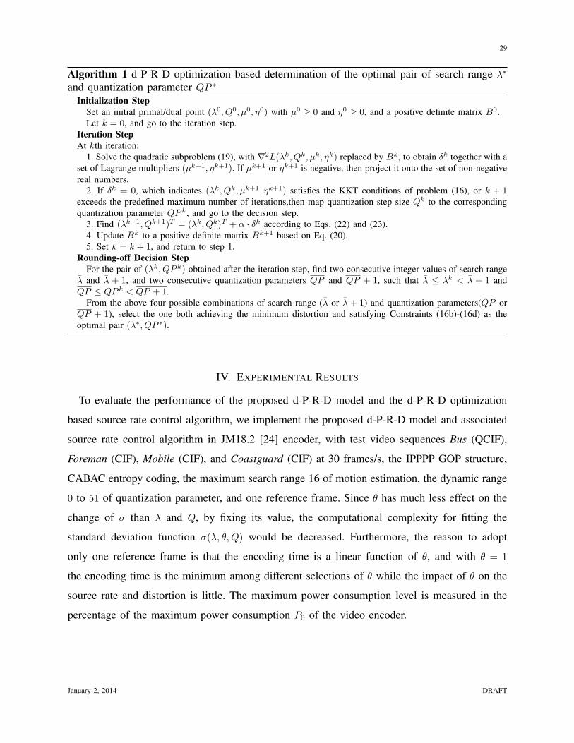
Algorithm 1 d-P-R-D optimization based determination of the optimal pair of search range λ∗

and quantization parameter QP ∗

Initialization StepSet an initial primal/dual point (λ0, Q0, µ0, η0) with µ0 ≥ 0 and η0 ≥ 0, and a positive definite matrix B0.Let k = 0, and go to the iteration step.

Iteration StepAt kth iteration:

1. Solve the quadratic subproblem (19), with ∇2L(λk, Qk, µk, ηk) replaced by Bk, to obtain δk together with aset of Lagrange multipliers (µk+1, ηk+1). If µk+1 or ηk+1 is negative, then project it onto the set of non-negativereal numbers.

2. If δk = 0, which indicates (λk, Qk, µk+1, ηk+1) satisfies the KKT conditions of problem (16), or k + 1exceeds the predefined maximum number of iterations,then map quantization step size Qk to the correspondingquantization parameter QP k, and go to the decision step.

3. Find (λk+1, Qk+1)T = (λk, Qk)T + α · δk according to Eqs. (22) and (23).4. Update Bk to a positive definite matrix Bk+1 based on Eq. (20).5. Set k = k + 1, and return to step 1.

Rounding-off Decision StepFor the pair of (λk, QP k) obtained after the iteration step, find two consecutive integer values of search range

λ and λ + 1, and two consecutive quantization parameters QP and QP + 1, such that λ ≤ λk < λ + 1 andQP ≤ QP k < QP + 1.

From the above four possible combinations of search range (λ or λ+ 1) and quantization parameters(QP orQP + 1), select the one both achieving the minimum distortion and satisfying Constraints (16b)-(16d) as theoptimal pair (λ∗, QP ∗).

IV. EXPERIMENTAL RESULTS

To evaluate the performance of the proposed d-P-R-D model and the d-P-R-D optimization

based source rate control algorithm, we implement the proposed d-P-R-D model and associated

source rate control algorithm in JM18.2 [24] encoder, with test video sequences Bus (QCIF),

Foreman (CIF), Mobile (CIF), and Coastguard (CIF) at 30 frames/s, the IPPPP GOP structure,

CABAC entropy coding, the maximum search range 16 of motion estimation, the dynamic range

0 to 51 of quantization parameter, and one reference frame. Since θ has much less effect on the

change of σ than λ and Q, by fixing its value, the computational complexity for fitting the

standard deviation function σ(λ, θ,Q) would be decreased. Furthermore, the reason to adopt

only one reference frame is that the encoding time is a linear function of θ, and with θ = 1

the encoding time is the minimum among different selections of θ while the impact of θ on the

source rate and distortion is little. The maximum power consumption level is measured in the

percentage of the maximum power consumption P0 of the video encoder.


30

A. Convergence Behavior and Model Accuracy

Figs. 13 and 14 show the convergence behavior of the proposed d-P-R-D optimization based

source rate control (RC) algorithm for the first 10 frames of a video sequence. Here, the maximum

power consumption level is set to 100%, i.e., Pmax = P0. It can be seen that by the proposed RC

algorithm, both primal (λ,Q) and dual variables (µ, η) can simultaneously and quickly converge

to the corresponding optimal values in a few iterations. If the initial values of λ and Q are closer

to the optimal solution, fewer number of iterations is needed for convergence. Within each

iteration, on the other hand, it is only required to solve a quadratic programming optimization

problem. In comparison, with the bi-section search algorithm [16], both the feasible region of

dual variables µ and η need an iterative bi-section search, which greatly increases the number

of iterations. Within each iteration of the bi-section search algorithm, the entire feasible sets of

primal variables λ and Q are exhaustively searched in order to find the optimal solution, which

means that the duration of one iteration is much longer than that of the proposed RC algorithm.

Take Fig. 13 as an example, with the proposed RC algorithm, only 5 iterations are needed to

converge to the optimal solution under three different initialization configurations. It is observed

from experiments on Bus sequence that, when the feasible ranges for µ and η are both set to

[0, 50], 13 iterations are required for convergence with bi-section search algorithm. Furthermore,

the number of iterations for convergence would become larger when the upper-bounds for µ

and η increase. Therefore, the computational complexity of the proposed RC algorithm is much

lower than the bi-section search algorithm.

In Fig. 13, the maximum source bit rate and encoding delay for Bus video sequence are set

to 1 bpp and 2.5 s, respectively. After the rounding-off decision of the proposed RC algorithm,

the minimum achievable distortion is 30.83 with the optimal parameters λ∗ = 12 and QP ∗ = 29

(Q∗ = 18). As validation, when the feasible sets of search range and QP are exhaustively searched

for the first 10 frames, the minimum distortion 31.35 is achieved with optimal parameters λ∗ = 11

and QP ∗ = 29 (Q∗ = 18). Similarly, the maximum source bit rate and encoding delay for the

Foreman video sequence in Fig. 14 are set to 0.1 bpp and 2.5 s, respectively. The minimum

distortion by the proposed RC algorithm is 23.47 with λ∗ = 2 and QP ∗ = 32 (Q∗ = 26), while

the true distortion obtained by the exhaustive search for the first 10 frames is 21.14 with λ∗ = 1

and QP ∗ = 32 (Q∗ = 26). Therefore, the proposed RC algorithm can achieve the near-optimal


31

0 2 4 6 8 105

10

15

20

25

30

35Bus

Iteration index k

Sea

rch

rang

e λ

λ

0=16,Q

0=10,µ

0=1,η

0=1

λ0=32,Q

0=1,µ

0=10,η

0=10

λ0=5,Q

0=20,µ

0=50,η

0=50

(a)

0 2 4 6 8 100

2

4

6

8

10

12

14

16

18

20Bus

Iteration index k

Qua

ntiz

atio

n st

ep s

ize

Q

λ0=16,Q

0=10,µ

0=1,η

0=1

λ0=32,Q

0=1,µ

0=10,η

0=10

λ0=5,Q

0=20,µ

0=50,η

0=50

(b)

0 2 4 6 8 100

10

20

30

40

50

60Bus

Iteration index k

Lagr

ange

mul

tiplie

r µ

λ0=16,Q

0=10,µ

0=1,η

0=1

λ0=32,Q

0=1,µ

0=10,η

0=10

λ0=5,Q

0=20,µ

0=50,η

0=50

(c)

0 2 4 6 8 100

5

10

15

20

25

30

35

40

45

50Bus

Iteration index k

Lagr

ange

mul

tiplie

r η

λ

0=16,Q

0=10,µ

0=1,η

0=1

λ0=32,Q

0=1,µ

0=10,η

0=10

λ0=5,Q

0=20,µ

0=50,η

0=50

(d)

Fig. 13. Convergence behavior of (a) search range λ, (b) quantization step size Q, and Lagrange multipliers (c) µ and (d) ηfor Bus sequence, where θ = 1, Rmax = 1 bpp, dmax = 2.5 s, and Pmax = P0 is the maximum power consumption level ofthe video encoder, with three different sets of initial values.

performance in practice. Comparing Figs. 13 and 14, it can be further observed that for the same

encoding delay constraint, a greater source bit rate is taken to encode Bus sequence yet yields a

higher distortion than Foreman sequence, which is derived from the fact that the motion in Bus

sequence is faster than Foreman sequence.

Fig 15 illustrates the true 3-D Pareto surface and the estimated 3-D Pareto surface by the

proposed RC algorithm of source distortion D, source rate R and encoding time d, when the

maximum power consumption level is set to 100%. A point on the 3-D Pareto surfaces indicates

the minimum achievable distortion associated with given rate and encoding time constraints. It


32

0 2 4 6 8 100

5

10

15

20

25

30

35Foreman

Iteration index k

Sea

rch

rang

e λ

λ

0=16,Q

0=2,µ

0=1,η

0=1

λ0=32,Q

0=1,µ

0=2,η

0=2

λ0=5,Q

0=5,µ

0=5,η

0=5

(a)

0 2 4 6 8 100

5

10

15

20

25Foreman

Iteration index k

Qua

ntiz

atio

n st

ep s

ize

Q

λ0=16,Q

0=2,µ

0=1,η

0=1

λ0=32,Q

0=1,µ

0=2,η

0=2

λ0=5,Q

0=5,µ

0=5,η

0=5

(b)

0 2 4 6 8 100

20

40

60

80

100

120

140

160Foreman

Iteration index k

Lagr

ange

mul

tiplie

r µ

λ0=16,Q

0=2,µ

0=1,η

0=1

λ0=32,Q

0=1,µ

0=2,η

0=2

λ0=5,Q

0=5,µ

0=5,η

0=5

(c)

0 2 4 6 8 100

5

10

15

20

25

30

35

40Foreman

Iteration index k

Lagr

ange

mul

tiplie

r η

λ0=16,Q

0=2,µ

0=1,η

0=1

λ0=32,Q

0=1,µ

0=2,η

0=2

λ0=5,Q

0=5,µ

0=5,η

0=5

(d)

Fig. 14. Convergence behavior of (a) search range λ, (b) quantization step size Q, and Lagrange multipliers (c) µ and (d) ηfor Foreman sequence, where θ = 1, Rmax = 0.1 bpp, dmax = 2.5 s, Pmax = P0 is the maximum power consumption levelof the video encoder, with three different sets of initial values.

can also be seen that the model estimation of the proposed RC algorithm is quite accurate.

B. d-P-R-D Model Analysis

To view the proposed d-P-R-D model in more detail, Fig. 16 illustrates the D-R curves for

different maximum encoding times, and D-d curves for different maximum source bit rates,

when the maximum power consumption level is set to 100%. As the D-R curves in Figs. 16(a)

and 16(c), for a given dmax, Dmin is a decreasing function of Rmax and such curve becomes

flat when Rmax is relatively large, which corresponds to Shannon’s source coding theory [37]. It

is noted that the previous work on rate control shows only one D-R curve of the similar shape


33

12

34

5

0

2

4

6

0

50

100

150

200

250

Encoding time (s)

Bus

Rate (bpp)

Dis

tort

ion

(MS

E)

True minimum distortion

(a)

12

34

5

0

2

4

6

0

50

100

150

200

250

Encoding time (s)

Bus

Rate (bpp)

Dis

tort

ion

(MS

E)

Estimated minimum distortion

(b)

3.5

4

4.5

5

0

2

4

6

0

10

20

30

40

50

Encoding time (s)

Foreman

Rate (bpp)

Dis

tort

ion

(MS

E)

True minimum distortion

(c)

3.5

4

4.5

5

0

2

4

6

0

10

20

30

40

Encoding time (s)

Foreman

Rate (bpp)

Dis

tort

ion

(MS

E)

Estimated minimum distortion

(d)

Fig. 15. 3-D Pareto surface of D, R, and d with Pmax = P0 being the maximum power consumption level of the videoencoder.

as Figs. 16(a) and 16(c). This is because that within their D-R models, the encoding time as

well as encoding power are always assumed to be fixed but unspecified, which is a special case

of the proposed d-P-R-D model. Hence in these work, the standard deviation σ of transformed

residuals is fixed as a result of fixed λ and θ, and their rate control is to tune QP since D and

R are functions of QP alone. From the D-d curves in Figs. 16(b) and 16(d), it can be seen that

Dmin decreases with dmax but becomes quite flat for larger dmax. This is because that ME has

already achieved a global optimal motion vector at a certain value of search range, and hence

continuously increasing the search range beyond that value contribute little to the decrement of

minimum achievable distortion.


34

1 1.5 2 2.5 30

5

10

15

20

25

30

35

40

Bit rate (bpp)

Dis

tort

ion

(MS

E)

Bus

d

max=0.8 s

dmax

=1 s

dmax

1.5 s

dmax

=2 s

(a)

0.8 1 1.2 1.4 1.6 1.8 2 2.2 2.40

5

10

15

20

25

30

35

40

45

50

Encoding time (s)

Dis

tort

ion

(MS

E)

Bus

R

max=1bpp

Rmax

=1.5 bpp

Rmax

=2 bpp

Rmax

=3 bpp

(b)

0 0.5 1 1.5 20

5

10

15

20

25

30

Bit rate (bpp)

Dis

tort

ion

(MS

E)

Foreman

d

max=2.1 s

dmax

=2.4 s

dmax

2.7 s

dmax

=3 s

(c)

2.2 2.4 2.6 2.8 3 3.2 3.4 3.6 3.8 40

5

10

15

20

25

30

35

Encoding time (s)

Dis

tort

ion

(MS

E)

Foreman

R

max=0.2 bpp

Rmax

=0.4 bpp

Rmax

=0.7 bpp

Rmax

=1 bpp

(d)

Fig. 16. D-R curves of (a) Bus sequence and (c) Foreman sequence for different maximum encoding times dmax, and D-dcurves of (b) Bus sequence and (c) Foreman sequence for different maximum bit rates Rmax, where Pmax = P0 is the maximumpower consumption level of the video encoder.

Fig. 17 shows the D-R curves for different maximum power consumption levels, and D-P

curves for different maximum source bit rates, with the maximum encoding delay fixed at 1 s

and 4 s for Bus and Foreman sequences. It can be seen from Figs. 17(a) and 17(c) that for a

given maximum power consumption level, the relationship of distortion and rate complies with

Shannon’s source coding theory. As illustrated by the D-P curves in Figs. 17(b) and 17(d), Dmin

decreases with the increment of the percentage of power consumption but becomes quite flat

for larger power consumption level. The reason is same as the previous analysis, i.e., ME has

already achieved an global optimal motion vector at a certain value of search range when the

power consumption level is relatively large.


35

1 1.5 2 2.5 30

10

20

30

40

50

60

70

Bit rate (bpp)

Dis

tort

ion

(MS

E)

Bus

100% power consumption75% power consumption50% power consumption25% power consumption

(a)

30 40 50 60 70 80 90 1000

10

20

30

40

50

60

70

Percentage of power consumption (%)

Dis

tort

ion

(MS

E)

Bus

R

max=1 bpp

Rmax

=1.5 bpp

Rmax

=2 bpp

Rmax

=3 bpp

(b)

0 0.5 1 1.5 20

2

4

6

8

10

12

14

16

18

20

22

Bit rate (bpp)

Dis

tort

ion

(MS

E)

Foreman

100% power consumption75% power consumption50% power consumption25% power consumption

(c)

20 30 40 50 60 70 80 90 1000

5

10

15

20

25


Dis

tort

ion

(MS

E)

Foreman

R

max=0.1 bpp

Rmax

=0.4 bpp

Rmax

=0.7 bpp

Rmax

=1 bpp

(d)

Fig. 17. D-R curves of (a) Bus sequence and (c) Foreman sequence for different power consumption levels Pmax, and D-Pcurves of (b) Bus sequence and (c) Foreman sequence for different maximum bit rates Rmax, where dmax for Bus sequenceand Foreman sequence are set to 1 s and 4 s, respectively.

Fig. 18 presents the D-d curves for different maximum power consumption levels, and D-P

curves for different maximum encoding times, with the maximum source bit rate fixed at 1.5

bpp and 0.5 bpp for Bus and Foreman sequences. It can be seen that the similar analysis of

the proposed d-P-R-D model is witnessed as well, i.e., Dmin decreases with dmax but becomes

quite flat for larger dmax, and Dmin decreases with the increment of the percentage of power

consumption but becomes quite flat for larger power consumption level.

C. Performance Comparison

In order to demonstrate the performance of the proposed RC algorithm, the d-P-R-D model is

derived from the first 10 frames of a video sequence and the proposed RC algorithm acts on the


36

0.8 1 1.2 1.4 1.6 1.8 2 2.2 2.415

20

25

30

35

40

Encoding time (s)

Dis

tort

ion

(MS

E)

Bus

100% power consumption75% power consumption50% power consumption

(a)

10 20 30 40 50 60 70 80 90 10015

20

25

30

35

40


Dis

tort

ion

(MS

E)

Bus

d

max=0.8 s

dmax

=1 s

dmax

=1.5 s

dmax

=2 s

(b)

2.5 3 3.5 40

10

20

30

40

50

60

Encoding time (s)

Dis

tort

ion

(MS

E)

Foreman

100% power consumption75% power consumption50% power consumption

(c)

40 50 60 70 80 90 1005

6

7

8

9

10

11

12


Dis

tort

ion

(MS

E)

Foreman

d

max=2.4 s

dmax

=2.7 s

dmax

=3 s

(d)

Fig. 18. D-d curves of (a) Bus sequence and (c) Foreman sequence for different power consumption levels Pmax, and D-Pcurves of (b) Bus sequence and (c) Foreman sequence for different maximum encoding times dmax, where Rmax for Bussequence and Foreman sequence are set to 1.5 bpp and 0.5 bpp, respectively.

entire video sequence. It should be noted that, when a new video scene is acquired, a new model

σ(λ,Q) = ae−b + c + dQ needs to be fitted with three fitting parameters a, b and c. In order to

have a better fitting result, in this paper, we have used the whole set of the empirical values with

different configurations of λ and Q to determine the three fitting parameters, which may cause

the increase in computational complexity higher. To reduce such complexity in practice, since

the function form of σ(λ,Q) is already known and only three fitting parameters are unknown, we

could choose a much smaller subset of empirical values with only a few configurations of λ and

Q as training set and obtained the standard deviation model with the tradeoff of fitting accuracy.

On the other hand, in the proposed RC algorithm, we only need to use the first several P-frames


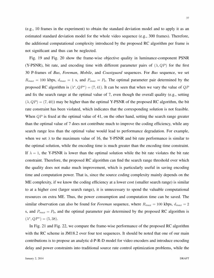
37

(e.g., 10 frames in the experiment) to obtain the standard deviation model and to apply it as an

estimated standard deviation model for the whole video sequence (e.g., 300 frames). Therefore,

the additional computational complexity introduced by the proposed RC algorithm per frame is

not significant and thus can be neglected.

Fig. 19 and Fig. 20 show the frame-wise objective quality in luminance-component PSNR

(Y-PSNR), bit rate, and encoding time with different parameter pairs of (λ,QP ) for the first

30 P-frames of Bus, Foreman, Mobile, and Coastguard sequences. For Bus sequence, we set

Rmax = 100 kbps, dmax = 1 s, and Pmax = P0. The optimal parameter pair determined by the

proposed RC algorithm is (λ∗, QP ∗) = (7, 41). It can be seen that when we vary the value of QP

and fix the search range at the optimal value of 7, even though the overall quality (e.g., setting

(λ,QP ) = (7, 40)) may be higher than the optimal Y-PSNR of the proposed RC algorithm, the bit

rate constraint has been violated, which indicates that the corresponding solution is not feasible.

When QP is fixed at the optimal value of 41, on the other hand, setting the search range greater

than the optimal value of 7 does not contribute much to improve the coding efficiency, while any

search range less than the optimal value would lead to performance degradation. For example,

when we set λ to the maximum value of 16, the Y-PSNR and bit rate performance is similar to

the optimal solution, while the encoding time is much greater than the encoding time constraint.

If λ = 1, the Y-PSNR is lower than the optimal solution while the bit rate violates the bit rate

constraint. Therefore, the proposed RC algorithm can find the search range threshold over which

the quality does not make much improvement, which is particularly useful in saving encoding

time and computation power. That is, since the source coding complexity mainly depends on the

ME complexity, if we know the coding efficiency at a lower cost (smaller search range) is similar

to at a higher cost (larger search range), it is unnecessary to spend the valuable computational

resources on extra ME. Thus, the power consumption and computation time can be saved. The

similar observation can also be found for Foreman sequence, where Rmax = 100 kbps, dmax = 2

s, and Pmax = P0, and the optimal parameter pair determined by the proposed RC algorithm is

(λ∗, QP ∗) = (5, 38).

In Fig. 21 and Fig. 22, we compare the frame-wise performance of the proposed RC algorithm

with the RC scheme in JM18.2 over four test sequences. It should be noted that one of our main

contributions is to propose an analytic d-P-R-D model for video encoders and introduce encoding

delay and power constraints into traditional source rate control optimization problems, while the


38

0 5 10 15 20 25 3022.5

23

23.5

24

24.5

25

25.5

Frame index

Y−

PS

NR

(dB

)Bus

Optimal λ*=7, QP*=41Set λ=1, QP=41Set λ=16, QP=41Set λ=7, QP=40Set λ=7, QP=42

(a)

0 5 10 15 20 25 3029.5

30

30.5

31

31.5

32

Frame index

Y−

PS

NR

(dB

)

Foreman


(b)

0 5 10 15 20 25 300

20

40

60

80

100

120

140

160

180

200

Frame index

Bit

rate

(kb

ps)

Bus

Optimal λ*=7, QP*=41

Set λ=1, QP=41

Set λ=16, QP=41

Set λ=7, QP=40

Set λ=7, QP=42

(c)

0 5 10 15 20 25 300

50

100

150

200

250

Frame index

Bit

rate

(kb

ps)

Foreman


(d)

0 5 10 15 20 25 300

0.5

1

1.5

2

2.5

3

3.5

4

4.5

Frame index

Enc

odin

g tim

e (s

)

Bus


(e)

0 5 10 15 20 25 301

2

3

4

5

6

7

8

9

10

Frame index

Enc

odin

g tim

e (s

)

Foreman


(f)

Fig. 19. (a), (b) The objective quality, (c), (d) bit rate and (e), (f) encoding time with different parameter pairs of (λ,QP ) forthe first 30 P-frames of Bus and Foreman sequences, where Rmax = 100 kbps, Pmax = P0 is the maximum power consumptionlevel of the video encoder, and dmax is set to 1 s and 2 s for Bus and Foreman sequences, respectively.


39

0 5 10 15 20 25 30

23

23.5

24

24.5

25

Frame index

Y−

PS

NR

(dB

)Mobile


Set λ=1, QP=41

Set λ=16, QP=41

Set λ=4, QP=40

Set λ=4, QP=42

(a)

0 5 10 15 20 25 3026

26.2

26.4

26.6

26.8

27

27.2

27.4

27.6

27.8

28

Frame index

Y−

PS

NR

(dB

)

Coastguard


Set λ=1, QP=39

Set λ=16, QP=39

Set λ=4, QP=38

Set λ=4, QP=40

(b)

0 5 10 15 20 25 300

100

200

300

400

500

600

700

800

Frame index

Bit

rate

(kb

ps)

Mobile


Set λ=1, QP=41

Set λ=16, QP=41

Set λ=4, QP=40

Set λ=4, QP=42

(c)

0 5 10 15 20 25 300

50

100

150

200

250

Frame index

Bit

rate

(kb

ps)

Coastguard


Set λ=1, QP=39

Set λ=16, QP=39

Set λ=4, QP=38

Set λ=4, QP=40

(d)

0 5 10 15 20 25 300

2

4

6

8

10

12

14

16

Frame index

Enc

odin

g tim

e (s

)

Mobile


Set λ=1, QP=41

Set λ=16, QP=41

Set λ=4, QP=40

Set λ=4, QP=42

(e)

0 5 10 15 20 25 300

2

4

6

8

10

12

14

16

Frame index

Enc

odin

g tim

e (s

)

Coastguard


(f)

Fig. 20. (a), (b) The objective quality, (c), (d) bit rate and (e), (f) encoding time with different parameter pairs of (λ,QP ) forthe first 30 P-frames of Mobile and Coastguard sequences, where dmax = 2 s, Pmax = P0 is the maximum power consumptionlevel of the video encoder, and Rmax is set to 500 kbps and 100 kbps for Mobile and Coastguard sequences, respectively.


40

0 5 10 15 20 25 3022

23

24

25

26

27

28

Frame index

Y−

PS

NR

(dB

)

Bus

Proposed RC, Initial QP=41JM RC, Initial QP=41Proposed RC, Initial QP=36JM RC, Initial QP=36Proposed RC, Initial QP=46JM RC, Initial QP=46

(a)

0 5 10 15 20 25 3028

29

30

31

32

33

34

Frame index

Y−

PS

NR

(dB

)

Foreman


(b)

0 5 10 15 20 25 300

50

100

150

200

250

300

Frame index

Bit

rate

(kb

ps)

Bus


(c)

0 5 10 15 20 25 300

50

100

150

200

250

300

350

400

450

Frame index

Bit

rate

(kb

ps)

Foreman


(d)

0 5 10 15 20 25 30

0.7

0.8

0.9

1

1.1

1.2

Frame index

Enc

odin

g tim

e (s

)

Bus


(e)

0 5 10 15 20 25 301

1.2

1.4

1.6

1.8

2

2.2

2.4

2.6

2.8

Frame index

Enc

odin

g tim

e (s

)

Foreman


(f)

Fig. 21. (a), (b) objective quality, (c), (d) bit rate and (e), (f) encoding time achieved by the proposed rate control algorithmand the rate control algorithm of JM with different setup of initial QP for the first I-frame, for the first 30 P-frames of Busand Foreman sequences, where search range is set to the optimal search range solved by the proposed algorithm, Rmax = 100kbps, Pmax = P0 is the maximum power consumption level of the video encoder, and dmax is set to 1 s and 2 s for Bus andForeman sequences, respectively.


41

0 5 10 15 20 25 3020

21

22

23

24

25

26

27

28

Frame index

Y−

PS

NR

(dB

)

Mobile


(a)

0 5 10 15 20 25 3024

25

26

27

28

29

30

31

Frame index

Y−

PS

NR

(dB

)

Coastguard


(b)

0 5 10 15 20 25 300

200

400

600

800

1000

1200

1400

Frame index

Bit

rate

(kb

ps)

Mobile


(c)

0 5 10 15 20 25 300

100

200

300

400

500

600

700

Frame index

Bit

rate

(kb

ps)

Coastguard


(d)

0 5 10 15 20 25 301.4

1.6

1.8

2

2.2

2.4

Frame index

Enc

odin

g tim

e (s

)

Mobile


(e)

0 5 10 15 20 25 301.2

1.4

1.6

1.8

2

2.2

2.4

Frame index

Enc

odin

g tim

e (s

)

Coastguard


(f)

Fig. 22. (a), (b) objective quality, (c), (d) bit rate and (e), (f) encoding time achieved by the proposed rate control algorithmand the rate control algorithm of JM with different setup of initial QP for the first I-frame, for the first 30 P-frames of Mobileand Coastguard sequences, where search range is set to the optimal search range solved by the proposed algorithm, dmax = 2s, Pmax = P0 is the maximum power consumption level of the video encoder, and Rmax is set to 500 kbps and 100 kbps forMobile and Coastguard sequences, respectively.


42

JM RC scheme fails to deal with the delay and power dimensions. In the JM RC scheme, the

control unit is a frame, and RDO is utilized based on an R-D model as a function of QP ,

such that by tuning respective QP of a frame it can meet the target bit rate while minimizing

the coding distortion. However, the delay and power constraints may not be satisfied since the

search range is not specified. To meet the maximum delay and power constraints and thus have

a “fair” comparison with the proposed RC scheme, here, we set the search range for the JM RC

scheme as the optimum value obtained by the proposed RC scheme.

It can be seen that, however, the performance of the JM RC scheme depends greatly on the

initial QP value of the first I-frame. According to [12], the selection of the initial quantization

step size for the first I-frame is very critical for model based rate control algorithm, since the rate-

distortion of the first frame can affect the coding efficiency of the subsequent frames. Therefore,

for JM rate control, if the initial quantization step size is set to be too small, the bit rate for

the first few frames would be much larger than the target bit rate. To make the average bit rate

meet the target bit rate, the bit rates allocated for the rest few frames would be much smaller by

increasing quantization step sizes for these frames. For example, for different setups of initial

QP for the first I-frame, the results of Y-PSNR, bit rate and encoding time per frame obtained

by the JM RC scheme are significantly different, while the results of the proposed RC algorithm

are relatively similar and not affected too much by different initial QP values. In addition, the

JM RC scheme fails to get a stable performance for the entire sequence which is required for a

better user experience. The corresponding Y-PSNR, bit rate, and encoding time vs. frame index

curves are quite fluctuated and unstable. Although the Y-PSNR values for some frames might

be higher than those of the proposed RC algorithm, the bit rate and encoding time constraints

are violated. In contrast, the selection of the initial quantization step size for the first I-frame

would have less impact on the performance of the proposed RC algorithm. The proposed RC

algorithm can achieve smooth and stable Y-PSNR performance while the other constraints are

satisfied.

The reason for the stability of the proposed RC algorithm is as follows. For each video

sequence, specifically, the proposed d-P-R-D model is derived based on the first several frames

and thus can characterize more accurately the statistics in that video sequence. When adopting

such d-P-R-D model in the proposed model based rate control algorithm, the optimal coding

parameters can be determined in accordance with different video sequences. And for each


43

TABLE ICOMPARISON OF AVERAGE Y-PSNR, BIT RATE AND ENCODING TIME (ET) UNDER DIFFERENT CONSTRAINTS OF MAXIMUM

POWER CONSUMPTION LEVELS, BIT RATE, ENCODING DELAY, AND DIFFERENT SETUP IN THE INITIAL QP FOR THE FIRSTI-FRAME, FOR THE FIRST 150 P-FRAMES OF Bus SEQUENCE.

Pmax (%) 100 50

dmax (s) 0.5 1 0.5 1

Rmax (kbps) 100 500 100 500 100 500 100 500Proposed Y-PSNR(dB) 23.38 29.93 23.56 30.79 22.58 29.10 23.51 30.77

RC Rate(kbps) 109.16 515.61 101.69 536.99 100.60 520.84 103.34 542.45QP ∗ ET(s) 0.49 0.45 0.95 1.10 0.51 0.49 1.01 0.99JM Y-PSNR(dB) 23.14 29.68 23.59 30.28 22.52 28.86 23.48 30.22RC Rate(kbps) 98.89 498.37 99.14 498.27 99.07 499.37 98.95 497.99QP ∗ ET(s) 0.49 0.44 0.94 1.07 0.52 0.49 0.99 0.96

Proposed Y-PSNR(dB) 23.44 29.95 23.63 30.84 22.56 29.12 23.57 30.82RC Rate(kbps) 110.61 515.92 102.58 536.93 101.99 516.42 103.16 541.58

QP ∗ − 10 ET(s) 0.49 0.46 0.93 1.09 0.51 0.47 1.01 0.97JM Y-PSNR(dB) 22.87 29.54 23.39 30.16 22.24 28.76 23.33 30.12RC Rate(kbps) 95.63 494.30 96.21 493.51 96.18 495.14 95.72 492.87

QP ∗ − 10 ET(s) 0.49 0.46 0.91 1.09 0.51 0.48 0.99 0.95Proposed Y-PSNR(dB) 23.44 29.92 23.53 30.81 22.58 29.12 23.52 30.80

RC Rate(kbps) 112.45 517.22 104.59 540.01 102.97 518.41 105.55 543.74QP ∗ + 10 ET(s) 0.50 0.47 0.94 1.11 0.51 0.50 1.01 0.99

JM Y-PSNR(dB) 22.75 29.60 23.15 30.22 22.21 28.75 23.07 30.16RC Rate(kbps) 100.53 502.33 100.39 501.89 100.50 502.34 100.75 502.08

QP ∗ + 10 ET(s) 0.48 0.46 0.92 1.08 0.52 0.49 1.00 0.96

sequence, λ∗ and Q∗ would remain the same for all frames, which makes the actual bit rate

and Y-PSNR more stable among different frames. For JM RC scheme, the quantization step size

is tuned and varied for each frame in accordance with general distortion-quantization (D-Q) and

rate-quantization (R-Q) models which are independent of different video contents. Therefore,

the optimal quantization step size determined by JM RC scheme would change frame by frame

in order to meet the target bit rate while minimizing the coding distortion. And the actual bit

rate and Y-PSNR would fluctuate with such change in quantization step size among different

frames.

Tables I-IV show the comparison of average Y-PSNR, bit rate, and encoding time for the first

150 P-frames of Bus, Foreman, Mobile, and Coastguard sequences, respectively. The maximum

achieved Y-PSNR results can verify the analysis of the d-P-R-D model in Sec. IV-B. It can also

be seen that the selection of the initial quantization step size for the first I-frame would have


44

TABLE IICOMPARISON OF AVERAGE Y-PSNR, BIT RATE AND ENCODING TIME (ET) UNDER DIFFERENT CONSTRAINTS OF MAXIMUM

POWER CONSUMPTION LEVELS, BIT RATE, ENCODING DELAY, AND DIFFERENT SETUP IN THE INITIAL QP FOR THE FIRSTI-FRAME, FOR THE FIRST 150 P-FRAMES OF Foreman SEQUENCE.

Pmax (%) 100 50

dmax (s) 2 3 2 3








QP ∗ + 10 ET(s) 2.10 2.07 3.05 2.86 1.94 1.99 3.02 3.15

less impact on the average Y-PSNR of the proposed RC scheme. That is, for the proposed RC

scheme, the average Y-PSNR performance under different selection of the initial quantization

step size is stable and usually better than that of the JM RC scheme. Although the mismatch of

the rate and encoding time may be a little larger at some times, most of them are still within a

certain tolerance region, say 10%, and the source rate and encoding time constraints can be still

considered as satisfied in practice.

V. CONCLUSION AND FUTURE WORK

In this paper, we derived the analytic delay-power-rate-distortion (d-P-R-D) model for IPPPP

coding mode in H.264/AVC to investigate the relationship among video encoding time, power,

rate and distortion. On the basis of the proposed d-P-R-D model, a model-based source rate

control problem has been formulated to minimize the encoding distortion under the constraints


45

TABLE IIICOMPARISON OF AVERAGE Y-PSNR, BIT RATE AND ENCODING TIME (ET) UNDER DIFFERENT CONSTRAINTS OF MAXIMUM

POWER CONSUMPTION LEVELS, BIT RATE, ENCODING DELAY, AND DIFFERENT SETUP IN THE INITIAL QP FOR THE FIRSTI-FRAME, FOR THE FIRST 150 P-FRAMES OF Mobile SEQUENCE.

Pmax (%) 100 50

dmax (s) 2 3 2 3








QP ∗ + 10 ET(s) 2.13 1.93 3.07 3.27 1.89 2.03 3.27 2.93

of rate, delay and power. To solve the rate control problem, we proposed a practical algorithm

to iteratively update the primal and dual variables by utilizing both the KKT conditions and the

SQP method. Experimental results have verified the accuracy of the proposed d-P-R-D model and

demonstrated the optimization performance of the model-based source rate control algorithm. The

d-P-R-D model and the model based rate control provided a theoretical basis and a practical

guideline for the cross-layer system design and performance optimization in wireless video

communication under delay and energy constraints. To further tackle the issue of bandwidth

fluctuations and higher packet losses in wireless transmissions, our future work will focus on

applying the proposed d-P-R-D approach to joint resource allocation and control for the entire

wireless video communication system, which aims at minimizing the end-to-end distortion under

the constraints of the transmission bandwidth, the end-to-end delay, and the total available power

supply of the wireless video communication system.


46

TABLE IVCOMPARISON OF AVERAGE Y-PSNR, BIT RATE, AND ENCODING TIME (ET) UNDER DIFFERENT CONSTRAINTS OF

MAXIMUM POWER CONSUMPTION LEVELS, BIT RATE, ENCODING DELAY, AND DIFFERENT SETUP OF THE INITIAL QP IN THEFIRST I-FRAME, FOR THE FIRST 150 P-FRAMES OF Coastguard SEQUENCE.

Pmax (%) 100 50

dmax (s) 2 3 2 3








QP ∗ + 10 ET(s) 2.07 1.92 2.69 3.14 2.13 1.97 3.02 2.91

APPENDIX A

PROOF OF EQUATIONS (5) AND (6)

The probability density function (pdf) of transform coefficients with i.i.d. zero-mean Laplacian

distribution is:

p(x) =1√2σ

e−√

2|x|σ =

Λ

2e−Λ|x| (24)

where x represents the transformed residual, σ is the standard deviation, and Λ =√2/σ is the

Laplace parameter. For the uniform quantizer with quantization step size Q and rounding offset

γQ, the probability of zero after quantization is

P0 =

∫ Q−γQ

−(Q−γQ)p(x)dx = 2

∫ Q(1−γ)

0p(x)dx = 1− e−ΛQ(1−γ) (25)


47

and the probability of transformed residuals inside nth quantization interval is

Pn =

∫ (n+1)Q−γQ

nQ−γQp(x)dx =

∫ Q(n+1−γ)

Q(n−γ)p(x)dx =

1

2(1− e−ΛQ)eΛQγe−ΛQn (26)

According to the entropy definition, therefore, the source rate can be approximated by the

entropy of the quantized transformed residuals, derived as

R(Λ, Q) = H(Λ, Q) = −P0 log2 P0 − 2

∞∑n=1

Pn log2 Pn (27)

= −P0 log2 P0 + (1− P0)

[ΛQ log2 e

1− e−ΛQ− log2(1− e−ΛQ)− ΛQγ log2 e+ 1

]On the other hand, the total quantization distortion is derived by summing up the quantization

distortion in each quantization interval as follows

D(Λ, Q) =

∫ Q−γQ

−(Q−γQ)x2p(x)dx+ 2

∞∑n=1

∫ (n+1)Q−γQ

nQ−γQ(x− nQ)2p(x)dx (28)

=ΛQeγΛQ(2 + ΛQ− 2γΛQ) + 2− 2eΛQ

Λ2(1− eΛQ)

APPENDIX B

DERIVATION OF EQUATION (19)

According to KKT conditions, the first-order necessary conditions of optimality for problem

Eq. (16) require the primal solutions (λ∗, Q∗) and dual solutions (µ∗, η∗) such that

∂L(λ∗, Q∗, µ∗, η∗)

∂λ=

∂D(λ∗, Q∗)

∂λ+ µ∗ · ∂R(λ∗, Q∗)

∂λ+ η∗ · ∂d(λ

∗, Q∗)

∂λ= 0 (29a)

∂L(λ∗, Q∗, µ∗, η∗)

∂Q=

∂D(λ∗, Q∗)

∂Q+ µ∗ · ∂R(λ∗, Q∗)

∂Q+ η∗ · ∂d(λ

∗, Q∗)

∂Q= 0 (29b)

d(λ∗, Q∗) =N(2λ∗ + 1)2θ · α(Q∗) · c0

3√

k−1Pmax

(29c)

µ∗ · [R(λ∗, Q∗)−Rmax] = 0 (29d)

η∗ · [d(λ∗, Q∗)− dmax] = 0 (29e)

Let us first consider using the Newton’s method to solve the set of nonlinear equations (34a)


48

- (34e), when µ∗ and η∗ are not equal to 0, as follows

∂L(λk, Qk, µk, ηk)

∂λ+

∂2L(λk, Qk, µk, ηk)

∂λ2(λk+1 − λk) +


∂λ∂Q(Qk+1 −Qk) (30a)

+∂R(λk, Qk)

∂λ(µk+1 − µk) +

∂d(λk, Qk)

∂λ(ηk+1 − ηk) = 0

∂L(λk, Qk, µk, ηk)

∂Q+


∂Q∂λ(λk+1 − λk) +


∂Q2(Qk+1 −Qk) (30b)

+∂R(λk, Qk)

∂Q(µk+1 − µk) +

∂d(λk, Qk)

∂Q(ηk+1 − ηk) = 0

R(λk, Qk)−Rmax +∂R(λk, Qk)

∂λ(λk+1 − λk) +

∂R(λk, Qk)

∂Q(Qk+1 −Qk) = 0 (30c)

d(λk, Qk)− dmax +∂d(λk, Qk)

∂λ(λk+1 − λk) +

∂d(λk, Qk)

∂Q(Qk+1 −Qk) = 0 (30d)

where a new iterate (λk+1, Qk+1, µk+1, ηk+1) is obtained by solving the first-order approximation,

given a current iterate (λk, Qk, µk, ηk). For all the defined functions, the derivative operators ∇

and ∇2, respectively, are used to refer to the first-order gradient and the second-order Hessian

matrix with respect to primal variables λ and Q. Furthermore, denoting δk = (δkλ, δkQ)

T = (λk+1−

λk, Qk+1 −Qk)T as the vector representing the update directions of primal variables, the set of

equations can be written as∇L(λk, Qk, µk, ηk)

R(λk, Qk)−Rmax

d(λk, Qk)− dmax

+

∇2L(λk, Qk, µk, ηk) ∇R(λk, Qk) ∇d(λk, Qk)

∇R(λk, Qk) 0 0

∇d(λk, Qk) 0 0

δk

µk+1 − µk

ηk+1 − ηk

= 0

(31)

Eq. (36) can be further written as∇2L(λk, Qk, µk, ηk) ∇R(λk, Qk) ∇d(λk, Qk)

∇R(λk, Qk) 0 0

∇d(λk, Qk) 0 0

δk

µk+1

ηk+1

=

−∇D(λk, Qk)

Rmax −R(λk, Qk)

dmax − d(λk, Qk)

(32)

At the kth iteration, the linear system in Eq. (37) can be solved for δk, µk+1, and ηk+1, and

then set (λk+1, Qk+1)T = (λk, Qk)T + δk for the next iteration. As the process is repeated until

δk = 0, we shall have found the stationary point to problem Eq. (16). Equivalently, given an

iterate (λk, Qk, µk, ηk), a new iterate (λk+1, Qk+1, µk+1, ηk+1) can also be obtained by solving a


49

quadratic programming (QP) minimization subproblem given by Eq. (19). It can be noted that the

optimum δk to Eq. (19), together with the optimal Lagrange multipliers µk+1 and ηk+1 associated

with the linearized constraints, is a stationary point for Eq. (19) and satisfies Eqs. (35a)-(35d)

when µk+1 and ηk+1 are grater than 0. In order to iteratively find an optimal solution for Eq.

(16), hence, Eq. (19) can be employed in lieu of the linear system (37).

REFERENCES

[1] Z. He, Y. Liang, L. Chen, I. Ahmad, and D. Wu, “Power-rate-distortion analysis for wireless video communication under

energy constraints,” IEEE Transactions on Circuits and Systems for Video Technology, vol. 15, no. 5, pp. 645–658, May

2005.

[2] Sandvine, “Global internet phenomena report,” 2012. [Online]. Available:

http://www.sandvine.com/downloads/documents/Phenomena 1H 2012/Sandvine Global Internet Phenomena Report 1H 2012.pdf

[3] “Global mobile data traffic forecast update, 2012-2017,” Cisco Visual Networking Index (VNI) Forecast, 2013. [Online].

Available: http://www.cisco.com/en/US/solutions/collateral/ns341/ns525/ns537/

ns705/ns827/white paper c11-520862.pdf

[4] X. Li, N. Oertel, A. Hutter, and A. Kaup, “Laplace distribution based Lagrangian rate distortion optimization for hybrid

video coding,” IEEE Transactions on Circuits and Systems for Video Technology, vol. 19, no. 2, pp. 193–205, Feb. 2009.

[5] C. Y. Hsu, A. Ortega, and M. Khansari, “Rate control for robust video transmission over burst-error wireless channels,”

IEEE Journal on Selected Areas in Communications, vol. 17, no. 5, pp. 756–773, May 1999.

[6] Q. Chen, “Image and video processing for denoising, coding, and content protection,” Ph.D. dissertation, University of

Florida, 2011.

[7] S. Soltani, K. Misra, and H. Radha, “Delay constraint error control protocol for real-time video communication,” IEEE

Transactions on Multimedia, vol. 11, no. 4, pp. 742–751, Jun. 2009.

[8] Q. Chen and D. Wu, “Delay-rate-distortion model for rea-time video communication,” submitted to IEEE Transactions on

Circuits and Systems for Video Technology for review, 2013.

[9] S. Khan, Y. Peng, E. Steinbach, M. Sgroi, and W. Kellerer, “Application-driven cross-layer optimization for video streaming

over wireless networks,” IEEE Communications Magazine, vol. 44, no. 1, pp. 122–130, Jan. 2006.

[10] Z. Li, F. Pan, K. Lim, G. Feng, X. Lin, and S. Rahardja, “Adaptive basic unit layer rate control for jvt,” in JVT-G012-r1,

7th Meeting, Pattaya II, Thailand, vol. 14, Mar. 2003.

[11] D. Kwon, M. Shen, and C. Kuo, “Rate control for H. 264 video with enhanced rate and distortion models,” IEEE

Transactions on Circuits and Systems for Video Technology, vol. 17, no. 5, pp. 517–529, May 2007.

[12] H. Wang and S. Kwong, “Rate-distortion optimization of rate control for H. 264 with adaptive initial quantization parameter

determination,” IEEE Transactions on Circuits and Systems for Video Technology, vol. 18, no. 1, pp. 140–144, Jan. 2008.

[13] B. Yan and K. Sun, “Joint complexity estimation of i-frame and p-frame for h. 264/avc rate control,” IEEE Transactions

on Circuits and Systems for Video Technology, vol. 22, no. 5, pp. 790–798, May 2012.

[14] S. Ma, W. Gao, and Y. Lu, “Rate-distortion analysis for H. 264/AVC video coding and its application to rate control,”

IEEE Transactions on Circuits and Systems for Video Technology, vol. 15, no. 12, pp. 1533–1544, Dec. 2005.

[15] I. E. G. Richardson, “H.264/MPEG-4 Part 10: Transform and Quantization,” 2003. [Online]. Available:

http://www.vcodex.com


50

[16] Z. Chen and D. Wu, “Rate-distortion optimized cross-layer rate control in wireless video communication,” IEEE

Transactions on Circuits and Systems for Video Technology, vol. 22, no. 3, pp. 352–365, Mar. 2012.

[17] A. Aminlou, Z. NajafiHaghi, M. Namaki-Shoushtari, and M. R. Hashemi, “Rate-distortion-complexity optimization for

vlsi implementation of integer motion estimation in h. 264/avc encoder,” in Proceedings of IEEE International Conference

on Multimedia and Expo. IEEE, 2011, pp. 1–6.

[18] J. Vanne, M. Viitanen, T. Hamalainen, and A. Hallpuro, “Comparative rate-distortion-complexity analysis of hevc and avc

video codecs,” IEEE Transactions on Circuits and Systems for Video Technology, vol. 22, no. 12, pp. 1885–1898, Dec.

2012.

[19] G. Correa, P. Assuncao, L. A. da Silva Cruz, and L. Agostini, “Adaptive coding tree for complexity control of high

efficiency video encoders,” in Picture Coding Symposium. IEEE, 2012, pp. 425–428.

[20] H. M. Hang and J. J. Chen, “Source model for transform video coder and its application. I. Fundamental theory,” IEEE

Transactions on Circuits and Systems for Video Technology, vol. 7, no. 2, pp. 287–298, Apr. 1997.

[21] G. S. Yovanof and S. Liu, “Statistical analysis of the DCT coefficients and their quantization error,” in Conference Record

of the 30th Asilomar Conference on Signals, Systems and Computers, vol. 1, Nov. 1996, pp. 601–605.

[22] N. Kamaci, Y. Altunbasak, and R. M. Mersereau, “Frame bit allocation for the H.264/AVC video coder via Cauchy-density-

based rate and distortion models,” IEEE Transactions on Circuits and Systems for Video Technology, vol. 15, no. 8, pp.

994–1006, Aug. 2005.

[23] T. Wiegand, G. J. Sullivan, G. Bjontegaard, and A. Luthra, “Overview of the H.264/AVC video coding standard,” IEEE

Transactions on Circuits and Systems for Video Technology, vol. 13, no. 7, pp. 560–576, Jul. 2003.

[24] K. Suhring, “H.264/AVC reference software JM18.2,” Feb. 2012. [Online]. Available:

http://iphome.hhi.de/suehring/tml/download/

[25] R. Min, T. Furrer, and A. Chandrakasan, “Dynamic voltage scaling techniques for distributed microsensor networks,” in

Proceedings of IEEE Computer Society Workshop on VLSI, 2000, pp. 43–46.

[26] J. R. Lorch, A. J. Smith et al., “Improving dynamic voltage scaling algorithms with PACE,” ACM SIGMETRICS

Performance Evaluation Review, vol. 29, no. 1, pp. 50–61, Jun. 2001.

[27] T. D. Burd and R. W. Brodersen, “Processor design for portable systems,” The Journal of VLSI Signal Processing, vol. 13,

no. 2, pp. 203–221, 1996.

[28] E. Lam and J. Goodman, “A mathematical analysis of the DCT coefficient distributions for images,” IEEE Transactions

on Image Processing, vol. 9, no. 10, pp. 1661–1666, Oct. 2000.

[29] S. P. Boyd and L. Vandenberghe, Convex optimization. Cambridge university press, 2004.

[30] H. Everett, “Generalized Lagrange multiplier method for solving problems of optimum allocation of resources,” Operations

research, vol. 11, no. 3, pp. 399–417, May–Jun. 1963.

[31] X. Li, N. Oertel, A. Hutter, and A. Kaup, “Advanced Lagrange multiplier selection for hybrid video coding,” in Proceedings

of IEEE International Conference on Multimedia and Expo. IEEE, 2007, pp. 364–367.

[32] Y. Shoham and A. Gersho, “Efficient bit allocation for an arbitrary set of quantizers,” IEEE Transactions on Acoustics,

Speech and Signal Processing, vol. 36, no. 9, pp. 1445–1453, Sep. 1988.

[33] A. Ortega and K. Ramchandran, “Rate-distortion methods for image and video compression,” IEEE Signal Processing

Magazine, vol. 15, no. 6, pp. 23–50, Nov. 1998.

[34] D. Bertsekas, Nonlinear programming. Athena Scientific, 1999.


51

[35] B. Chachuat, Nonlinear and dynamic optimization: From Theory to Practice. Switzerland: Automatic Control Laboratory,

EPFL, 2007.

[36] J. Nocedal and S. J. Wright, Numerical optimization. Springer, 2006.

[37] T. Cover and J. Thomas, Elements of information theory. Wiley-interscience, 2006.


delay-power-rate-distortion model for wireless video ... · 1 delay-power-rate-distortion model for...

Documents