on the contribution of the horizontal sea-bed ... › pdf › 1011.1741.pdfe-mail:...
TRANSCRIPT

arX
iv:1
011.
1741
v5 [
phys
ics.
clas
s-ph
] 1
2 Ju
l 201
2
ON THE CONTRIBUTION OF THE HORIZONTAL SEA-BED
DISPLACEMENTS INTO THE TSUNAMI GENERATION PROCESS
DENYS DUTYKH∗, DIMITRIOS MITSOTAKIS, LEONID B. CHUBAROV, AND YURIY I. SHOKIN
Abstract. The main reason for the generation of tsunamis is the deformation of the
bottom of the ocean caused by an underwater earthquake. Usually, only the vertical
bottom motion is taken into account while the horizontal co-seismic displacements are
neglected in the absence of landslides. In the present study we propose a methodology
based on the well-known Okada solution to reconstruct in more details all components of
the bottom coseismic displacements. Then, the sea-bed motion is coupled with a three-
dimensional weakly nonlinear water wave solver which allows us to simulate a tsunami
wave generation. We pay special attention to the evolution of kinetic and potential energies
of the resulting wave while the contribution of the horizontal displacements into wave
energy balance is also quantified. Such contribution of horizontal displacements to the
tsunami generation has not been discussed before, and it is different from the existing
approaches. The methods proposed in this study are illustrated on the July 17, 2006 Java
tsunami and some more recent events.
Contents
1. Introduction 12. Mathematical models 52.1. Dynamic bottom displacements reconstruction 52.2. The water wave problem with moving bottom 103. Numerical results 134. Discussion and conclusions 22Appendix A. Applications to some recent tsunami events 23A.1. Mentawai 2010 tsunami 23A.2. March 11, 2011 Japan earthquake and tsunami 24Acknowledgement 25References 25
1. Introduction
During the years 2004 to 2006 several interesting tsunami events took place in the IndianOcean. In December 26, 2004, the Great Sumatra-Andaman earthquake (Mw = 9.1, cf.
Key words and phrases. tsunami waves; water waves; coseismic displacements; wave energy; finite fault
inversion.∗ Corresponding author. Tel: +33 4 79 75 86 52, Fax: +33 4 79 75 81 42. E-mail:

2 D. DUTYKH, D. MITSOTAKIS, L. B. CHUBAROV, AND YU. I. SHOKIN
C. Ammon et al. (2005), [1]) generated the devastating Indian Ocean tsunami refered toin the literature as the Tsunami Boxing Day 2004 (cf. C. Synolakis & E. Bernard (2006),[83]). The local tsunami run-ups from this event exceeded the height of 34 m at Lhokngain the western Aceh Province. This and other observations led many researchers to askwhether this tsunami was unusualy large for this specific earthquake size. Later it wasshown by E.L. Geist et al. (2006) [32] that the Great Sumatra-Andaman earthquake isvery similar in terms of local tsunami magnitude to past events of the same size. Forexample, the 1964 Great Alaska earthquake (Mw = 9.2, cf. H. Kanamori (1970) [49])demonstrates a similar scaling.
On March 28, 2005 another earthquake occured approximately 110 km to the SE fromthe Great Sumatra-Andaman earthquake’s epicenter. The magnitude of this earthquakewas estimated to be Mw = 8.6 ∼ 8.7 (cf. [57, 8, 93]). This event triggered a massiveevacuation in the surrounding Indian Ocean countries. However, the March 28, 2005Northern Sumatra earthquake failed to generate a significant tsunami event. The surveyteams reported maximum tsunami run-up of 4 m. [32]. This event can be compared withthe 1957 Aleutian earthquake (Mw = 8.6, cf. J.M. Johnson and K. Satake (1993) [46])which produced a maximum tsunami run-up of 15 m (see J.F. Lander (1996) [55]). Thedeficiency of the March 2005 tsunami is related to the slip concentration in the down-dippart of the rupture zone and to the fact that a substantial part of the vertical displacementoccurred in shallow waters or on the substance of the ground [32].
On the other hand, the smaller July 16, 2006 Java earthquake (Mw = 7.8, cf. C.J. Am-mon et al. (2006), [2]) generated an unexpectedly destructive tsunami wave which affectedover 300 km of south Java coastline and killed more than 600 people, [26]. Field mea-surements of run-up distributions range uniformly from 5 to 7 m in most inundated areas.However, unexpectedly high run-up values were reported at Nusakambangan Island exceed-ing the value of 20 m. This tsunami focusing effect could be seemingly ascribed to localsite effects and/or to a local submarine landslide/slump. July 16, 2006 Java tsunami canbe compared to a similar event occured on June 2, 1994 at the East Java (Mw = 7.6) (seeY. Tsuji et al. (1995), [88]). This 1994 Java tsunami produced more than 200 casualtieswith local run-up at Rajekwesi slightly exceeding 13 m.
All these examples of recent and historical tsunami events show that there is a big varietyof the local tsunami heights and run-up values with respect to the earthquake magnitudeMw. It is obvious that the seismic moment M0 of underwater shallow earthquakes isadequate to estimate far-field tsunami amplitudes (see also [68]). However, tsunami waveenergy reflects better the local tsunami severity, while the specific run-up distributiondepends on bathymetric propagation paths and other site-specific effects. One of thecentral challenges in the tsunami science is to rapidly assess a local tsunami severity fromvery first rough earthquake estimations. In the current state of our knowledge false alarmsfor local tsunamis appear to be unavoidable. The tsunami generation modeling attemptsto improve our understanding of tsunami behaviour in the vicinity of the genesis region.
Tsunami generation modeling was initiated in the early sixties by the prominent workof K. Kajiura, [47], who proposed the use of the static vertical sea bed displacement

CONTRIBUTION OF HORIZONTAL DISPLACEMENTS INTO TSUNAMI GENERATION 3
for the initial condition of the free surface elevation. Classically, the celebrated Okada,[66, 67], and sometimes Mansinha & Smylie1 [59, 60] or Gusiakov,[33], solutions are usedto compute the coseismic sea bed displacements. This approach is still widely used by thetsunami wave modeling community. However, some progress has been recently made inthis direction,[65, 19, 18, 21, 74, 76, 25].
There is a consensus on the importance of the horizontal motion in landslide generatedtsunamis, [37, 95, 4, 69]. However, for tsunami waves caused by underwater earthquakes,the horizontal displacements are often disregarded by the tsunami wave modeling com-munity. We can quote here a few publications devoted to tsunami waves such as one byD. Stevenson (2005), [81]:
“Although horizontal displacements are often larger, they are unimportantfor tsunami generation except to the extent that the sloping ocean floor alsoforces a vertical displacement of the water column.”
Or another one by G.A. Ichinose et al. (2000) [41]:
“The initial lake level values were specified by assuming that the lake surfaceinstantaneously conformed to the vertical displacement of the lake bottomwhile horizontal velocities were set to zero. The effect of horizontal defor-mation on the initial condition is neglected here and left for future work.”
The authors of this article also tended to neglect the horizontal displacements field inprevious tsunami generation studies, [18, 64]. Perhaps, this situation can be ascribed tothe work of E. Berg (1970), [7], who showed in the case of the 1964 Alaska’s earthquake(Mw = 9.2) that the input into the potential energy from the horizontal motion is less than1.5% of that from the vertical movement.
The attitude to horizontal displacements changed after the prominent work by Y. Tan-ioka and K. Satake (1996), [84]. According to their computations for the 1994 Java earth-quake, the inclusion of horizontal displacements contribution results in 43% increase inmaximum initial vertical ground displacement and an increase in the wave amplitudes atthe shoreline by 30%. These striking results incited researchers to reconsider the role ofthe horizontal sea bed motion. Hereafter, various tsunami generation techniques whichinvolve only the vertical displacement field are referred to as the incomplete scenario. Onthe contrary, the complete tsunami generation takes also into account the horizontal dis-placements field. The term complete in our study refers to a purely kinematic interactionbetween the moving bottom and the ocean layer in contrast to the horizontal impulse-momentum transfer mechanism [91] applied for the first time to tsunami wave generationin [78].
The approach proposed by Tanioka & Satake (1996) is based on a simple physical con-sideration: horizontal displacements of a sloping bottom will produce some amount of thevertical motion depending on the slope magnitude. Assuming that the slope is small, thisidea can be expressed mathematically by applying once the first order Taylor expansion:
uh := u1hx + u2hy,
1In fact, Mansinha & Smylie solution is a particular case of the more general Okada solution.

4 D. DUTYKH, D. MITSOTAKIS, L. B. CHUBAROV, AND YU. I. SHOKIN
where u1,2 are the horizontal components of the displacements field and h(x, y) is thebathymetry function. The indices x and y denote the spatial partial derivatives. Tanioka& Satake (1996) referred to the quantity uh as the vertical displacement of water due to thehorizontal movement of the slope. Then, the quantity uh is simply added as a correction tothe vertical displacements component u3(x, y). To compute the co-seismic displacementsu1,2,3 they used the celebrated Okada solution [80, 66, 67] applied to a single rectangularfault segment. In the present study we apply the same solution to multiple sub-faultsto achieve higher resolution (see also [24]). More recently, an original approach based onthe impulse-momentum principle, [91], has been proposed in [78]. Their genesis theoryis based on the idea of the momentum exchange between the slipped continental slopeand the water column due to the earthquake. The horizontal bottom motion contributesdirectly to the ocean kinetic energy as any moving object in water transfers momentumto the fluid. This idea is similar to the classical added mass concept. According to theauthors of [78], the continental slope is not an exception from this principle. This impliessome special treatment of the water parcels in the vicinity of moving boundaries. For moredetails we refer to the original publication [78]. The horizontal impulse approach leads topredictions which are somehow different from the present and several previous studies. Themethodology described in this article is closer to the ideas of Tanioka & Satake (1996) [84].Namely, we reconstruct in more details the kinematics of bottom displacements in verticaland horizontal directions, including their evolution in time. We underline that most oftsunami generation studies, including [84], assume the bottom deformation process to beinstantaneous, that in most of the cases provides a fairly good approximation. Then, thebottom motion generates some perturbations on the free surface of the water layer. Thisperturbation form long waves, propagating across the oceans under the gravity force andcommonly referred to as tsunami waves due to their destructive potential fully realizedonly in coastal regions, [47, 89, 16, 83].
In the current study we shed some light into the energy transfer process from an under-water earthquake to the implied tsunami wave (in the spirit of the study by D. Dutykh& F. Dias (2009), [20]), while taking into account and quantifying the horizontal displace-ments contribution into tsunami energy balance. We focus only on the generation stagesince the propagation phase and run-up techniques are well understood nowadays at leastin the context of Nonlinear Shallow Water equations, [42, 14, 53, 25, 23].
The present study is organized as follows. In Section 2 we present mathematical modelsused in this study. Specifically, in Sections 2.1 and 2.2 a description of the bottom motionand the fluid layer solution is presented respectively. Some rationale on tsunami waveenergy computations is discussed in Section 2.2.1. Numerical results are presented inSection 3. Finally, some important conclusions of this study are outlined in Section 4. Inthe Appendix of this paper we present the results concerning the tsumami generation oftwo recent events.

CONTRIBUTION OF HORIZONTAL DISPLACEMENTS INTO TSUNAMI GENERATION 5
2. Mathematical models
Tsunami waves are caused by a huge and rapid motion of the seafloor due to an under-water earthquake over broad areas in comparison to water depth. There are some othermechanisms of tsunami genesis such as underwater landslides, for example. However, inthis study we focus on the purely seismic mechanism which occurs most frequently innature.
Hydrodynamics and seismology are only weakly coupled in the tsunami generation prob-lem. Namely, the released seismic energy is partially transmitted to the ocean through thesea bed deformation while the ocean has obviously no influence onto the rupturing process.Consequently, our problem is reduced to two relatively distinct questions:
(1) Reconstruct the sea bed deformation h = h(~x, t) caused by the seismic event underconsideration
(2) Compute the resulting free surface motion
The answers to these questions are analyzed in Sections 2.1 and 2.2 respectively.
2.1. Dynamic bottom displacements reconstruction. Traditionally, the free surfaceinitial condition for various tsunami propagation codes (see [85, 42, 43]) is assumed to beidentical to the static vertical deformation of the ocean bottom, [48]. This assumption isclassically justified by the three following reasons:
(1) Tsunamis are long waves. In this regime the vertical acceleration is neglected withrespect to the gravity force
(2) The sea bed deformation is assumed to be instantaneous. It is based on the com-parison of gravity wave speed (200 m/s for water depth of 4 km) and the seismicwave celerity (≈ 3600 m/s)
(3) The effect of horizontal bottom motion is negligible for tsunami generation sincethe bathymetry has in general mild slope (≈ 10%), [7]
It is worth to note that nonhydrostatic effects as well as finite time source duration havebeen modeled in several recent studies [87, 19, 28, 52, 21, 29]. Some attempts have alsobeen made to take into account the horizontal displacements contribution, [84, 32, 78].
In the present study we relax all three classical assumptions. The bottom deformationis reconstructed using the finite fault solution as it was suggested in our previous study[24]. However, we extend the previous construction to take into account the horizontaldisplacements contribution as well. The finite fault solution is based on the multi-faultrepresentation of the rupture, [5, 45]. The rupture complexity is reconstructed using theinversion of seismic data. Fault’s surface is parametrized by multiple segments with variablelocal slip, rake angle, rise time and rupture velocity. The inversion is performed in anappropriate wavelet transform space. The objective function is a weighted sum of L1, L2
norms and some correlative functions. With this approach seismologists are able to recoverrupture slip details, [5, 45]. This available seismic information is exploited hereafter tocompute the sea bed displacements produced by an underwater earthquake with bettergeophysical resolution. Several other multiple segments sources have been used in [31, 94,61].

6 D. DUTYKH, D. MITSOTAKIS, L. B. CHUBAROV, AND YU. I. SHOKIN
Figure 1. Surface projection of the fault’s plane and the ETOPO1 bathy-metric map of the region under consideration. The symbol ⋆ indicates thehypocenter’s location at (107.345,−9.295). The local Cartesian coordinatesystem is centered at the point (108,−10). This region is located between(106,−8) and (110,−12). The colorbar indicates the water depth in me-ters below the still water level (z = 0). In the region under considerationthe depth varies from 20 to 7100 meters.
Remark 1. In a few studies an attempt has been made to reconstruct the seismic sourcefrom tsunami tide gauge records, [71, 72, 97, 30, 40, 75]. This approach seems to be verypromising and in future a joint combination of seismic and hydrodynamic inversions shouldbe used for the successful reconstruction of appropriate initial conditions.
Let us describe the way of how the sea bed displacements are reconstructed. In thisreconstruction procedure we follow the great lines of our previous study [24], while addingnew ingredients concerning the horizontal displacements field reconstruction. We illustratethe proposed approach in the case of the July 17, 2006 Java tsunami for which the finitefault solution is available, cf. [44, 70]. It was a relatively slow earthquake and thus,atypical. However, we assume that the slow rupturing process was well resolved by thefinite fault inversion algorithm.
The fault is considered to be the rectangle with vertices located at (109.20508 (Lon),−10.37387 (Lat), 6.24795 km (Depth)), (106.50434, −9.45925, 6.24795 km), (106.72382,−8.82807, 19.79951 km), (109.42455, −9.74269, 19.79951 km) (see Figure 1). The fault’splane is conventionally divided into Nx = 21 subfaults along strike and Ny = 7 subfaults

CONTRIBUTION OF HORIZONTAL DISPLACEMENTS INTO TSUNAMI GENERATION 7
P -wave celerity cp, m/s 6000
S-wave celerity cs, m/s 3400
Crust density ρ, kg/m3 2700
Dip angle, δ 10.35
Slip angle (CW from N) 288.94
Table 1. Geophysical parameters used to model elastic properties of thesubduction zone in the region of Java.
down the dip angle, leading to the total number of Nx × Ny = 147 equal segments. Pa-rameters such as the subfault location (xc, yc), the depth di, the slip ui and the rake angleφi for each segment can be found in [44] (see also Appendix II, [24]). The elastic constantsand parameters such as dip and slip angles, which are common to all subfaults, are givenin Table 1. We underline that the slip angle is measured conventionally in the counter-clockwise direction from the North. The relations between the elastic wave celerities cp, csand Lame coefficients λ, µ used in Okada’s solution are classical and can also be found inAppendix III, [24].
One of the main ingredients in our construction is the so-called Okada solution, [66, 67],which is used in the case of an active fault of small or intermediate size. The success of thissolution may be ascribed to the closed-form analytical expressions which can be effectivelyused for various modeling purposes involving co-seismic deformation.
Remark 2. The celebrated Okada solution, [66, 67], is based on two main ingredients— the dislocation theory of Volterra [92, 80] and Mindlin’s fundamental solution for anelastic half-space, [63]. Particular cases of this solution were known before Okada’s work,for example the well-known Mansinha and Smylie’s solution, [59, 60]. Usually all theseparticular cases differ by the choice of the dislocation and the Burger’s vector orientation,[73]. We recall the basic assumptions behind this solution:
• Fault is immersed into the linear homogeneous and isotropic half-space• Fault is a Volterra’s type dislocation• Dislocation has a rectangular shape
For more information on Okada’s solution we refer to [19, 16, 18] and the references therein.
The trace of the Okada’s solution at the sea bottom (substituting z = 0 in the geophysical
coordinate system) for each subfault will be denoted O(j)i (~x; δ, λ, µ, . . .), where δ is the dip
angle, λ, µ are the Lame coefficients and dots denote the dependence of the function O(j)i (~x)
on other 8 parameters, cf. [19]. The index i takes values from 1 to Nx×Ny and denotes thecorresponding subfault segment, while the superscript j is equal to 1 or 2 for the horizontaldisplacements and to 3 for the vertical component. Hereafter we will adopt the short-hand
notation O(j)i (~x) for the jth displacement component of the Okada’s solution for the ith
segment having in mind its dependence on various parameters.Taking into account the dynamic characteristics of the rupturing process, we make some
further assumptions on the time dependence of the displacement fields. The finite fault
8 D. DUTYKH, D. MITSOTAKIS, L. B. CHUBAROV, AND YU. I. SHOKIN
solution provides us with two additional parameters concerning the rupture kinematics —the rupture velocity vr and the rise time tr which are equal to 1.1 km/s and 8 s for July 17,2006 Java event respectively. The epicenter is located at the point ~xe = (107.345,−9.295),cf. [44]. Given the origin ~xe, the rupture velocity vr and ith subfault location ~xi, we definethe subfault activation times ti needed for the rupture to achieve the corresponding segmenti by the formulas:
ti =||~xe − ~xi||
vr, i = 1, . . . , Nx ×Ny.
Consequently, for the sake of simplicity in our study we assume the rupture propagationalong the fault to be isotropic and homogeneous. However, some more sophisticated ap-proaches including possible heterogeneities exist (see e.g. [13]). We will also follow thepioneering idea of J. Hammack, [36, 35], developed later in [87, 86, 19, 22, 52], where themaximum bottom deformation is achieved during some finite time (the so-called rise time)according to an appropriately chosen dynamic scenario. Various scenarios used in practice(instantaneous, linear, trigonometric, exponential, etc) can be found in [36, 50, 35, 22, 19].In this study we adopt the trigonometric scenario which is given by the following formula:
T (t) = H(t− tr) +1
2H(t)H(tr − t)
(1− cos(πt/tr)
), (2.1)
where H(t) is the Heaviside step function. This scenario has the advantage to have also thefirst derivative continuous at the activation time t = 0. However, for comparative purposessometimes we will use also the so-called exponential scenario [50]:
Te(t) = H(t)(1− e−αt
), α :=
log(3)
tr.
For illustrative purposes both dynamic scenarios are represented in Figure 2.We sum up together all the ingredients proposed above to reconstruct dynamic displace-
ments field ~u = (u1, u2, u3) at the sea bottom:
uj(~x, t) =
Nx×Ny∑
i=1
T (t− ti)O(j)i (~x).
Remark 3. We would like to underline here the asymptotic behaviour of the sea bed dis-placements. By definition of the trigonometric scenario (2.1) we have lim
t→+∞T (t) = 1.
Consequently, the sea bed deformation will attain fast its state which consists of the linearsuperposition of subfaults contributions:
uj(~x, t) =
Nx×Ny∑
i=1
O(j)i (~x).
Finally, we can predict the sea bed motion by taking into account horizontal and verticaldisplacements:
h(~x, t) = h0(~x− ~u1,2(~x, t))− u3(~x, t), (2.2)

CONTRIBUTION OF HORIZONTAL DISPLACEMENTS INTO TSUNAMI GENERATION 9
−0.5 0 0.5 1 1.5 2 2.5 3 3.5 4
0
0.1
0.2
0.3
0.4
0.5
0.6
0.7
0.8
0.9
1
t, s
T(t
)Dynamic scenarios
Trigonometric scenario
Exponential scenario
Figure 2. Trigonometric and exponential dynamic scenarios for tr = 1 s(see J. Hammack (1973), [35]).
where h0(~x) is a function which interpolates2 the static bathymetry profile given e.g. bythe ETOPO1 database (see Figures 1 and 4).
Remark 4. In some studies where horizontal displacements were taken into account (cf.[84, 3, 78, 6]), the first order Taylor expansion was permanently applied to the bathymetryrepresentation formula (2.2) to give:
h(~x, t) ≈ h0(~x)− ~u1,2(~x, t) · ∇~xh0(~x)− u3(~x, t) (2.3)
We prefer not to follow this approximation and to use the exact formula (2.2) since itis valid for all slopes (see Figure 4 for Java bathymetry). Another difficulty lies in theestimation of the bathymetry gradient ∇~xh0(x) required by Taylor’s formula (2.3). Theapplication of any finite differences scheme to the measured h0(~x) leads to an ill-posedproblem. Consequently, one needs to apply extensive smoothing procedures to the raw datah0(~x) which induces an additional loss in accuracy.
In the present study we do not completely avoid the computation of the static bathymetrygradient ∇~xh0(~x) since the kinematic bottom boundary condition (2.7) involves the timederivative of the bathymetry function:
∂th = −∇~xh0(~x) · ∂t~u1,2(~x, t)− ∂tu3(~x, t).
2In our numerical simulations presented below we use the MATLAB TriScatteredInterp class to
interpolate the static bathymetry values given by ETOPO1 database.

10 D. DUTYKH, D. MITSOTAKIS, L. B. CHUBAROV, AND YU. I. SHOKIN
However, the last formula is exact and it is obtained by a straightforward application of thechain differentiation rule.
Another possibility could be to consider static horizontal displacements ~u1,2(~x) thus keep-ing dynamics only in the vertical component u3(~x, t). However, we do not choose thisoption in this work.
In the next section we will present our approach in coupling this dynamic deformationwith the hydrodynamic problem to predict waves induced on the free surface of the ocean.
2.2. The water wave problem with moving bottom. We consider the incompressibleflow of an ideal fluid with constant density ρ in the domain Ω ⊆ R
2. The horizontalindependent variables will be denoted by ~x = (x, y) and the vertical one by z. The originof the Cartesian coordinate system is traditionally chosen such that the surface z = 0corresponds to the still water level. The fluid domain is bounded below by the bottomz = −h(~x, t) and above by the free surface z = η(~x, t). Usually we assume that the totaldepth H(~x, t) := h(~x, t) + η(~x, t) remains positive H(~x, t) ≥ h0 > 0 under the systemdynamics ∀t ∈ [0, T ]. The sketch of the physical domain is shown in Figure 3.
Remark 5. Classically in water wave modeling, we make the assumption that the freesurface is a graph z = η(~x, t) of a single-valued function. It means in practice that weexclude some interesting phenomena, (e.g. wave breaking phenomena) which are out of thescope of this modeling paradigm.
The governing equations of the classical water wave problem are the following, [54, 82,62, 96]:
∆φ = ∇2φ+ ∂2zzφ = 0, (~x, z) ∈ Ω× [−h, η], (2.4)
∂tη +∇φ · ∇η − ∂zφ = 0, z = η(~x, t), (2.5)
∂tφ+ 12|∇φ|2 + 1
2(∂zφ)
2 + gη = 0, z = η(~x, t), (2.6)
∂th +∇φ · ∇h + ∂zφ = 0, z = −h(~x, t), (2.7)
where φ is the velocity potential, g the acceleration due to gravity force and ∇ = (∂x, ∂y)denotes the gradient operator in horizontal Cartesian coordinates. The fluid incompressibil-ity and flow irrotationality assumptions lead to the Laplace equation (2.4) for the velocitypotential φ(~x, z, t).
The main difficulty of the water wave problem lies on the boundary conditions. Equations(2.5) and (2.7) express the free surface and bottom impermeability, while the Bernoullicondition (2.6) expresses the free surface isobarity respectively.
Function h(~x, t) represents the ocean’s bathymetry (depth below the still water level,see Figure 3) and is assumed to be known. The dependence on time is included in order totake into account the bottom motion during an underwater earthquake [16, 19, 22, 52, 18].
For the exposition below we will need also to compute unitary exterior normals to thefluid domain. The normals at the free surface Sf and at the bottom Sb are given by the

CONTRIBUTION OF HORIZONTAL DISPLACEMENTS INTO TSUNAMI GENERATION 11
−4−3
−2−1
01
23
4
−4
−3
−2
−1
0
1
2
3
4
−2
−1.5
−1
−0.5
0
0.5
z
x
y
O
η (x,y,t)
h(x,y,t)
h0
a
Figure 3. Sketch of the physical domain.
following expressions respectively:
nf =1
√
1 + |∇η|2
∣∣∣∣
−∇η1
, nb =1
√
1 + |∇h|2
∣∣∣∣
−∇h−1
.
In 1968 V. Zakharov proposed a different formulation of the water wave problem basedon the trace of the velocity potential at the free surface [98]:
ϕ(~x, t) := φ(~x, η(~x, t), t).
This variable plays a role of the generalized momentum in the Hamiltonian description ofwater waves [98, 15]. The second canonical variable is the free surface elevation η.
Another important ingredient is the normal velocity at the free surface vn which isdefined as:
vn(~x, t) :=√
1 + |∇η|2∂φ
∂nf
∣∣∣∣z=η
= (∂zφ−∇φ · ∇η)|z=η . (2.8)
Kinematic and dynamic boundary conditions (2.5), (2.6) at the free surface can be rewrittenin terms of ϕ, vn and η [12, 11, 27]:
∂tη −Dη(ϕ) = 0,
∂tϕ+ 12|∇ϕ|2 + gη − 1
2(1+|∇η|2)
[Dη(ϕ) +∇ϕ · ∇η
]2= 0.
(2.9)

12 D. DUTYKH, D. MITSOTAKIS, L. B. CHUBAROV, AND YU. I. SHOKIN
Here we introduced the so-called Dirichlet-to-Neumann operator (D2N) [10, 11] which mapsthe velocity potential at the free surface ϕ to the normal velocity vn:
Dη : ϕ 7→ vn =√
1 + |∇η|2 ∂φ
∂nf
∣∣∣z=η
∣∣∣∣∣∣∣∣
∇2φ+ ∂2zzφ = 0, (~x, z) ∈ Ω× [−h, η],φ = ϕ, z = η,
√
1 + |∇h|2∂φ
∂nb
= ∂th, z = −h.
The name of this operator comes from the fact that it makes a correspondance between
Dirichlet data ϕ and Neumann data√
1 + |∇η|2∂φ
∂nf
∣∣∣∣z=η
at the free surface.
So, the water wave problem can be reduced to a system of two PDEs (2.9) governingthe evolution of the canonical variables η and ϕ. For the tsunami generation problem weapproximate and we compute efficiently the D2N map Dη(ϕ) using the Weakly Nonlinear(WN) model described in [24]. This relies on the approximate solution of the 3D Laplaceequation in a perturbed strip-like domain using the Fourier transform (ϕ := F [ϕ], η =F−1[η]):
Dη(ϕ) = ϕ|~k| tanh(|~k|H) + f sech(|~k|H)−F[
F−1[i~kϕ
]· F−1
[i~kη
]]
,
where ~k is the wavenumber and f is the bathymetry forcing term
f(~x, t) := −∂th− ∇φ|z=−h · ∇h.
Several details on the time integration procedure can be also found in [24]. The resultingmethod is only weakly nonlinear and analogous at some point to the first order approxima-tion model proposed in [34]. As the hydrodynamical models, Tanioka and Satake (1996)[84] used the Linear Shallow Water equations [77], while Song et al. (2008) employed ahydrostatic ocean circulation model [79].
Recently, it was shown that a tsunami generation process is essentially linear, [52, 76].However, our WN approach will take into account some nonlinear effects when they becomeimportant, for example when rapid changes in the bathymetry are present. This is possiblewhen the generation region involves a wide range of depths from deep to shallow regions(see Figures 1 and 4).
2.2.1. Tsunami wave energy. In this study we are more particularly interested in the evolu-tion of the generated wave energy [20]. In the case of free surface incompressible flows, thekinetic and potential energies, denoted by K and Π respectively, are completely determinedby the velocity field and the free surface elevation:
K(t) :=ρ
2
η∫
−h
∫∫
Ω
|∇φ|2 d~x dz, Π(t) :=ρg
2
∫∫
Ω
η2 d~x.
The definition of the kinetic energy K(t) involves an integral over the three dimensionalphysical domain Ω× [−h, η]. We can reduce the integral dimension using the fact that the

CONTRIBUTION OF HORIZONTAL DISPLACEMENTS INTO TSUNAMI GENERATION 13
velocity potential φ is a harmonic function:
|∇φ|2 = ∇ · (φ∇φ)− φ ∆φ︸︷︷︸
=0
≡ ∇ · (φ∇φ).
Consequently, the kinetic energy can be rewritten as follows:
K(t) =ρ
2
∫∫
Sf+Sb
φ∇φ · n dσ =ρ
2
∫∫
Ω
ϕDη(ϕ) d~x
︸ ︷︷ ︸
(I)
+ρ
2
∫∫
Ω
φ∂th d~x
︸ ︷︷ ︸
(II)
,
where φ denotes the trace of the velocity potential at the bottom φ|z=−h (see D. Clamond& D. Dutykh (2012), [9]). In order to obtain the last equality we used the free surface andthe bottom kinematic boundary conditions (2.6), (2.7). The first integral (I) is classicaland represents the change of kinetic energy under the free surface motion while the secondone (II) is the forcing term due to the bottom deformation. The total energy3 is definedas the sum of kinetic and potential ones:
E(t) := K(t) + Π(t) =ρ
2
∫∫
Ω
ϕDη(ϕ) d~x+ρ
2
∫∫
Ω
φ∂th d~x+ρg
2
∫∫
Ω
η2 d~x.
Below we will compute the evolution of the kinetic, potential and total energies beneathmoving bottom.
3. Numerical results
The proposed approach will be directly illustrated on the Java 2006 event. The July17, 2006 Java earthquake involved thrust faulting in the Java’s trench and generated atsunami wave that inundated the southern coast of Java, [2, 26]. The estimates of the sizeof the earthquake, [2], indicate a seismic moment of 6.7×10²⁰ N ·m, which corresponds tothe magnitude Mw = 7.8. Later this estimation was refined to Mw = 7.7, [44]. Like otherevents in this region, Java’s event had an unusually low rupture speed of 1.0 – 1.5 km/s(we take the value of 1.1 km/s according to the finite fault solution [44]), and occurrednear the up-dip edge of the subduction zone thrust fault. According to C. Ammon et al,[2], most aftershocks involved normal faulting. The rupture propagated approximately 200km along the trench with an overall duration of approximately 185 s. The fault’s surfaceprojection along with ocean ETOPO1 bathymetric map are shown in Figures 1 and 4. Wenote that Indian Ocean’s depth of the region considered in this study varies between 7186and 20 meters in the shallowest regions which may imply local importance of nonlineareffects.
Remark 6. We have to mention that the finite fault inversion for this earthquake wasalso performed by the Caltech team, [70]. The main differences with the USGS inversionconsist on the employed dataset. To our knowledge, A. Ozgun Konca and his collaboratorsinclude also displacements measured with GPS-based techniques. Consequently, they came
3We note that the total energy is not conserved during the tsunami generation phase due to the forcing
term (II) coming from the bottom kinematic boundary condition.

14 D. DUTYKH, D. MITSOTAKIS, L. B. CHUBAROV, AND YU. I. SHOKIN
Figure 4. Side view of the bathymetry, cf. also Figure 1.
Ocean water density, ρ, kg/m3 1027.0
Gravity acceleration, g, m/s2 9.81
Epicenter location (Lon, Lat) (107.345, -9.295)
Rupture velocity, vr, km/s 1.1
Rise time, t0, s 8.0
Number of Fourier modes in x 256
Number of Fourier modes in y 256
Table 2. Values of physical and numerical parameters used in simulations.
to the conclusion that the July 17, Southern Java earthquake magnitude was Mw = 7.9.The energy of a tsunami wave generated according to this solution will be discussed below.
The numerical solutions presented below are given by the Weakly Nonlinear (WN) model.A uniform grid of 256 × 256 points4 is used in all computations below. The time step ∆tis chosen adaptively according to the RK(4,5) method proposed in [17]. The problemis integrated numerically during T = 255 s which is a sufficient time interval for thebottom to take its final shape (< 220 s) and of the resulting tsunami wave to enter into
4Since we use a pseudo-spectral method, the convergence is expected to be exponential and this number
of harmonics should be sufficient to capture all scales important for phenomena that we consider here.
CONTRIBUTION OF HORIZONTAL DISPLACEMENTS INTO TSUNAMI GENERATION 15
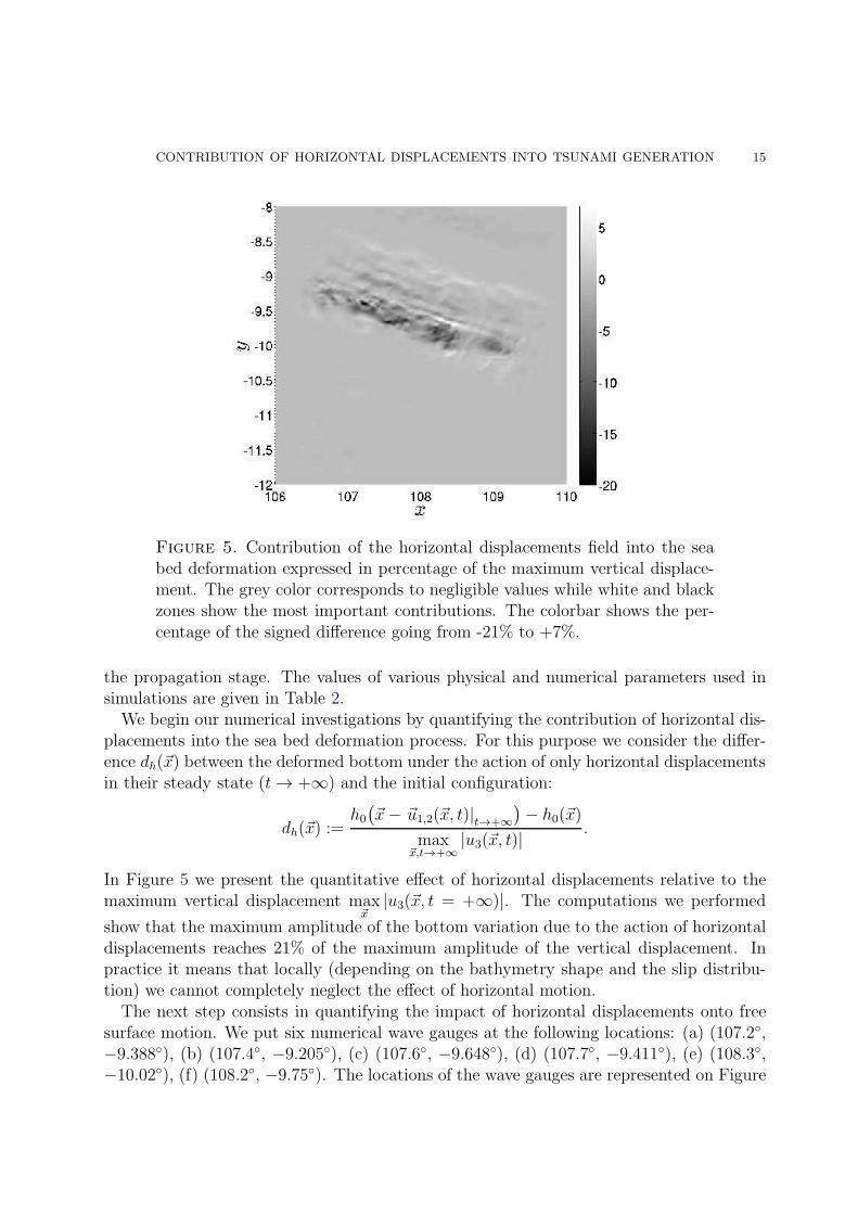
Figure 5. Contribution of the horizontal displacements field into the seabed deformation expressed in percentage of the maximum vertical displace-ment. The grey color corresponds to negligible values while white and blackzones show the most important contributions. The colorbar shows the per-centage of the signed difference going from -21% to +7%.
the propagation stage. The values of various physical and numerical parameters used insimulations are given in Table 2.
We begin our numerical investigations by quantifying the contribution of horizontal dis-placements into the sea bed deformation process. For this purpose we consider the differ-ence dh(~x) between the deformed bottom under the action of only horizontal displacementsin their steady state (t → +∞) and the initial configuration:
dh(~x) :=h0
(~x− ~u1,2(~x, t)|t→+∞
)− h0(~x)
max~x,t→+∞
|u3(~x, t)|.
In Figure 5 we present the quantitative effect of horizontal displacements relative to themaximum vertical displacement max
~x|u3(~x, t = +∞)|. The computations we performed
show that the maximum amplitude of the bottom variation due to the action of horizontaldisplacements reaches 21% of the maximum amplitude of the vertical displacement. Inpractice it means that locally (depending on the bathymetry shape and the slip distribu-tion) we cannot completely neglect the effect of horizontal motion.
The next step consists in quantifying the impact of horizontal displacements onto freesurface motion. We put six numerical wave gauges at the following locations: (a) (107.2,−9.388), (b) (107.4, −9.205), (c) (107.6, −9.648), (d) (107.7, −9.411), (e) (108.3,−10.02), (f) (108.2, −9.75). The locations of the wave gauges are represented on Figure

16 D. DUTYKH, D. MITSOTAKIS, L. B. CHUBAROV, AND YU. I. SHOKIN
Figure 6. Location of the six numerical wave gauges (indicated by thesymbol ⋄) superposed with the steady state coseismic bottom displacement(only the vertical component in meters is represented here).
6 along with the static sea bed displacement. Wave gauges are intentionally put in placeswhere the largest waves are expected. Synthetic wave gauge records are presented in Figure7. We consider the following four scenarios:
• trigonometric, complete (blue solid line)• trigonometric, incomplete (black dashed line)• exponential, complete (blue dash-dotted line)• exponential, incomplete (black dotted line)
The importance of the nonlinear effects have already been addressed in several previousstudies, [52, 76]. In the framework of the Weakly Nonlinear approach we studied thisquestion in a recent companion paper [24] using only the vertical deformation. A fairly goodagreement has been observed with the Cauchy-Poisson (linear, fully dispersive) formulationin accordance with preceding results, cf. [52, 76]. Consequently, in the present study wedecided to focus on the further comparison between complete/incomplete approaches andexponential/trigonometric scenarios, [35, 22, 64]. These results are discussed hereafter.
We note that the trigonometric scenario leads in general to slightly larger amplitudesthan the exponential bottom motion. It is not surprising since the exponential scenarioprescribes smoother and less rapid change in the bottom for the same rise time parametervalue (see Figure 2). Later we will consider the trigonometric scenario unless otherwisenoted.
Then, it can be seen that in most cases horizontal displacements lead to an increase inthe wave amplitude but not always as it can be observed in Figure 7(f) (the last wavegauge located at (108.2,−9.75)). We investigated more thoroughly this question. Fig-ure 8 shows the relative difference between free surface elevations computed according to

CONTRIBUTION OF HORIZONTAL DISPLACEMENTS INTO TSUNAMI GENERATION 17
0 50 100 150 200 250−0.2
−0.1
0
0.1
0.2
0.3
0.4
t
η(t)
Gauge 1
Complete, trig.Incomplete, trig.Complete, exp.Incomplete, exp.
(a) Gauge at (107.2,−9.388)
0 50 100 150 200 250−0.2
−0.1
0
0.1
0.2
0.3
0.4
t
η(t)
Gauge 2
Complete, trig.Incomplete, trig.Complete, exp.Incomplete, exp.
(b) Gauge at (107.4,−9.205)
0 50 100 150 200 250−0.2
−0.1
0
0.1
0.2
0.3
0.4
t
η(t)
Gauge 3
Complete, trig.Incomplete, trig.Complete, exp.Incomplete, exp.
(c) Gauge at (107.6,−9.648)
0 50 100 150 200 250−0.2
−0.1
0
0.1
0.2
0.3
0.4
t
η(t)
Gauge 4
Complete, trig.Incomplete, trig.Complete, exp.Incomplete, exp.
(d) Gauge at (107.7,−9.411)
0 50 100 150 200 250−0.2
−0.1
0
0.1
0.2
0.3
0.4
0.5
t
η(t)
Gauge 5
Complete, trig.Incomplete, trig.Complete, exp.Incomplete, exp.
(e) Gauge at (108.3,−10.02)
0 50 100 150 200 250−0.2
−0.1
0
0.1
0.2
0.3
0.4
t
η(t)
Gauge 6
Complete, trig.
Incomplete, trig.
Complete, exp.
Incomplete, exp.
(f) Gauge at (108.2,−9.75)
Figure 7. Free surface elevations computed numerically at six wave gaugeslocated approximately in local extrema of the static bottom displacement.The vertical axis is represented in meters and time is given in seconds. Theblack lines correspond to the wave generated only by the vertical displace-ments (incomplete generation) while blue lines take also into account thehorizontal displacements contribution (complete scenario).

18 D. DUTYKH, D. MITSOTAKIS, L. B. CHUBAROV, AND YU. I. SHOKIN
Figure 8. Relative difference between the free surface elevation at te = 220seconds computed according to the complete ηc(~x, te) (with horizontal dis-placements) and incomplete ηi(~x, te) (only vertical component) tsunami gen-eration scenarios. The bottom moves according to the trigonometric scenario(2.1). The vertical scale is given in percents of the maximum amplitude ofthe incomplete scenario — max
~xηi(~x, te).
complete ηc(~x, te) and incomplete ηi(~x, te) scenarios. More precisely, we plot the followingquantity (for the trigonometric scenario):
d(~x) :=ηc(~x, te)− ηi(~x, te)
max~x
|ηi(~x, te)|, te = 220 s.
Time te = 220 s has been chosen because at that moment the bottom has been stabilizedand the waves enter into the free propagation regime. In Figure 8 the grey color correspondsto the zero value of the difference d(~x), while the white color shows regions where the waveis amplified by horizontal displacements by approximately 10%. On the contrary, blackzones show an attenuation effect of horizontal sea bed motion (about −5%). Recall thatall values are given in terms of the maximum amplitude max
~x|ηi(~x, te)| percentage of the
incomplete generation approach. Some connection with the results presented in Figure 5can be noticed.
Finally, we study the evolution of kinetic, potential and total energies during the tsunamigeneration process described in Section 2.2.1. Specifically we are interested in quantifyingthe contribution of horizontal displacements into tsunami energy balance. Figure 9 showsthe evolution of potential (9(a)) and kinetic (9(b)) energies for four cases already mentioned

CONTRIBUTION OF HORIZONTAL DISPLACEMENTS INTO TSUNAMI GENERATION 19
0 50 100 150 200 2500
2
4
6
8
10
12
14x 10
11
t
P(t
), J
Potential energy
Complete, trig.
Incomplete, trig.
Complete, exp.
Incomplete, exp.
(a) Potential energy Π(t), J
0 50 100 150 200 2500
0.5
1
1.5
2
2.5
3
3.5x 10
12
t
K(t
), J
Kinetic energy
Complete, trig.Incomplete, trig.Complete, exp.Incomplete, exp.
(b) Kinetic energy K(t), J
Figure 9. Energy evolution during our simulations in the complete (bluesolid line) and incomplete (black dotted line) scenarios. Note that scales aredifferent on the left and right images. The time t is given in seconds.
above. Here again blue lines refer to complete generation scenarios while black lines –to vertical displacements only. Consecutive peaks in the kinetic energy come from theactivation of new fault segments in accordance with the rupture propagation along the fault.The energy curves vary in an analogous way with the tide gauges records (see Figure 7).Namely, the trigonometric scenario leads to slightly higher energies than the exponentialone. However, once the bottom motion stops, this difference becomes negligible. Theinclusion of horizontal displacements has a much more visible effect with higher energies.
We performed also the same simulation but using the finite fault solution obtained bythe Caltech team, [70], and the trigonometric scenario. The results concerning the kineticand potential energies are presented in Figure 10. It is interesting to note that the potentialenergy evolution in the Caltech scenario appears to be smoother especially after t = 150s. However, the peaks corresponding to subfaults activation times are equally present inkinetic energies. The magnitudes of kinetic and potential energies predicted accordingto the Caltech inversion are approximatively 10 times higher than corresponding USGSresults.
We have to underline that inversions performed by the two different finite fault algo-rithms lead to very different results. Our method is operational with both of them. Itis particularly interesting to compare the total energies evolution predicted by USGS andCaltech inversions. These results are presented in Figure 11. The Caltech version of therupturing process generates a tsunami wave with much higher energy (computed after theend of the bottom motion when a tsunami enters in the propagation regime):
• USGS, complete trigonometric: Ec = 2.16× 10¹² J,• USGS, complete exponential: Ec = 2.11× 10¹² J,• USGS, incomplete trigonometric: Ei = 1.95× 10¹² J,

20 D. DUTYKH, D. MITSOTAKIS, L. B. CHUBAROV, AND YU. I. SHOKIN
0 50 100 150 200 2500
2
4
6
8
10
12
14
16
18x 10
12
t
P(t
), J
Potential energy
Complete, trig.
Incomplete, trig.
(a) Potential energy Π(t), J
0 50 100 150 200 2500
1
2
3
4
5
6
7
8
9
10x 10
12
t
K(t
), J
Kinetic energy
Complete, trig.
Incomplete, trig.
(b) Kinetic energy K(t), J
Figure 10. Energy evolution during our simulations in the complete (bluesolid line) and incomplete (black dotted line) scenarios using the finite faultinversion by Caltech Tectonics Observatory [70]. Note that the scales aredifferent on the left and right images. The time t is given in seconds.
• USGS, incomplete exponential: Ei = 1.90× 10¹² J,• Caltech, complete trigonometric: Ec = 2.28× 10¹³ J,• Caltech, incomplete trigonometric: Ec = 1.83× 10¹³ J.
This result is not surprising since according to the USGS solution the Java 2006 eventmagnitude is Mw = 7.7 and according to the Caltech team, Mw = 7.9, which means a hugedifference since the scale is logarithmic.
Remark 7. We would like to note an interesting property. For linear waves it can be rigor-ously shown the exact equipartition property between the kinetic and potential energies [96].When the nonlinearities are included, this equidistribution property is only approximate.One can observe that at the final time in our simulations the kinetic and potential energiesare already of the same order of magnitude regardless the employed bottom motion (seeFigures 9 & 10). Moreover, both curves K(t) and Π(t) continue to tend to the equilibriumstate according to the theoretical predictions of the water wave theory, [96].
Despite some local attenuation effects of horizontal displacements on the free surfaceelevation, the complete generation scenario produces a tsunami wave with more importantenergy content. More precisely, our computations show that the horizontal displacementscontribute about 10% into the total tsunami energy balance in the USGS scenario (thisvalue is consistent with our previous results concerning the differences in wave amplitudesin Figure 8). This result is even more flagrant for the Caltech version which ascribes 24%of the energy to horizontal displacements. The free surface amplitudes in this case shoulddiffer as well by the same order of magnitude. As we already noted, the difference betweentrigonometric and exponential scenarios is negligible.

CONTRIBUTION OF HORIZONTAL DISPLACEMENTS INTO TSUNAMI GENERATION 21
0 50 100 150 200 2500
0.5
1
1.5
2
2.5
3
3.5
4
4.5x 10
12
t
E(t
), J
Total energy
Complete, trig.
Incomplete, trig.
Complete, exp.
Incomplete, exp.
(a) USGS version
0 50 100 150 200 2500
0.5
1
1.5
2
2.5x 10
13
t
P(t
), J
Total energy
Complete, trig.
Incomplete, trig.
(b) Caltech version
Figure 11. The total energy evolution predicted according to two differentversions of the finite fault inversion. Note the different vertical scales on left(4.5× 10¹²) and right (2.5× 10¹³) images. The time t is given in seconds.
Up to now the contribution of horizontal displacements has been quantified in termsof the bottom deformation (Figure 5), free surface elevation at a particular moment oftime (t = 220 s, cf. Figure 8) and finally in terms of the wave energy (Figures 9 –11). However, the wave energy cannot be directly measured in practice. Consequently,we continue to quantify the differences between complete and incomplete approaches interms of the waveforms. Namely, we compute also the following relative measures of thewaveforms difference which act on the whole computed free surface:
d2(t) :=||ηc(~x, t)− ηi(~x, t)||L2(R2)
||ηi(~x, t)||L2(R2)
, d∞(t) :=||ηc(~x, t)− ηi(~x, t)||L∞(R2)
||ηi(~x, t)||L∞(R2)
. (3.1)
The simulation results are presented on Figure 12. One can see that both measures grow upto 15% and then oscillate around this level, at least during the simulation time. This resultis in agreement with previous measurements of the horizontal displacements contributionbased on the wave energy and the bottom deformation which were of the order of 10%. Wenote also that the curve d2(t) has a more regular behaviour than d∞(t) since it is based onintegral characteristics of the difference while the latter focusses on the characteristics ofthe extreme values.
It is also interesting to compare the tsunami energy with the energy of the underlyingseismic event. The USGS Energy and Broadband solution indicates that the radiatedseismic energy of the Java 2006 earthquake is equal to 3.2 × 10¹⁴ J. Hence, according toour computations with the USGS complete generation approach and the trigonometricscenario, about 0.68% of the seismic energy was transmitted to the tsunami wave (thisportion raises to 7.14% for the Caltech version). The ratio of the total tsunami andseismic radiated energies can be used as a measure of the tsunami generation efficiencyof a specific earthquake. The seismic radiated energy may not be the most appropriate

22 D. DUTYKH, D. MITSOTAKIS, L. B. CHUBAROV, AND YU. I. SHOKIN
50 100 150 200 2507
8
9
10
11
12
13
14
15
16
17
t, s
d2,∞(t),%
Relative difference between free surface elevations
d2(t)
d∞(t)
Figure 12. Relative difference between free surface elevations computedaccording to the complete and incomplete scenarios. For more details seeequation (3.1). The horizontal axis is given in seconds, while the verticalscale is a percentage. The blue solid line (—) corresponds to the measured2(t). The black dashed line (−−−) represents d∞(t).
parameter to use, but it has an advantage to be relatively robust and easily observable incontrast to the more relevant seismic fracture energy, [90, 51].
This parameter can also be estimated for the Great Sumatra-Andaman earthquake ofDecember 26, 2004. The total energy of the Great Indian Ocean tsunami 2004 was esti-mated by T. Lay et al. (2005), [57], to be equal to 4.2 × 10¹⁵ J. According to the sameUSGS Energy and Broadband solution the radiated seismic energy was equal to 1.1× 10¹⁷
J. Thus, the tsunamigenic efficiency of the Great Sumatra-Andaman earthquake is 3.81%which is bigger than that of Java 2006 event but remains in the same order of magnitudearound 1%. It is possible that we do not still take into account all important factors inJava 2006 tsunami genesis. More examples of transmission of seismic energy to tsunamienergy can be found e.g. in [58].
4. Discussion and conclusions
In the present study the process of tsunami generation is further investigated. Thecurrent tsunamigenesis model relies on a combination of the finite fault solution,[45], and arecently proposed Weakly Nonlinear (WN) solver for the water wave problem with movingbottom, [24]. Consequently, in our model we incorporate recent advances in seismologyand computational hydrodynamics.
This study is focused on the role of the horizontal displacements in the real world tsunamigenesis process. By our intuition we know that a horizontal motion of the flat bottom willnot cause any significant disturbance on the free surface. However, the real bathymetry

CONTRIBUTION OF HORIZONTAL DISPLACEMENTS INTO TSUNAMI GENERATION 23
is far from being flat. The question which arises naturally is how to quantify the effect ofhorizontal co-seismic displacements during real world events.
The primary goal of this study was to propose relatively simple, efficient and accurateprocedures to model tsunami generation process in realistic environments. Special emphasiswas payed to the role of horizontal displacements which should be also taken into account.Thus, the kinematics of horizontal co-seismic displacements were reconstructed and theireffect on free surface motion was quantified. The evolution of kinetic and potential energieswere also investigated in our study. In the case of July 17, 2006 Java event our simulationsindicate that 10% of the energy input can be seemingly ascribed to effects of the horizontalbottom motion. This portion increases considerably if we switch to the scenario proposedby Caltech Tectonics Observatory [70].
The results presented in this study do not still explain the reasons for the extreme run-upvalues caused by July 17, 2006 Java tsunami, [26]. At least we hope that the proposedmethodology illustrated on this important real world event will be proved helpful in fu-ture studies. In our opinion a successful theory should incorporate also other generationmechanisms such as local landslides/slumps which are subject to large uncertainties at thecurrent stage of our understanding. Until now there are no detailed images of the seabedwhich could support or disprove this assumption. In this study we succeeded to quantifythe significance of horizontal displacements for the tsunami generation.
Appendix A. Applications to some recent tsunami events
In this Appendix we apply the techniques described in this manuscript to two recentsignificant events. We compute the energy transmission from the corresponding seismicevent to the resulting tsunami wave with and without horizontal displacements. Through-out this Appendix we use the trigonometric scenario and the finite fault solutions producedby USGS.
Remark 8. In later versions of the finite fault solution the activation and rise time, aswell as the seismic moment are specified for each sub-fault. Consequently, below we usethis information to produce more accurate bottom kinematics. It allows us to compute alsothe seismic moment rate function5.
A.1. Mentawai 2010 tsunami. In October 25, 2010 a small portion of the subductionzone seaward of the Mentawai islands was ruptured by an earthquake of magnitude Mw =7.7, [56]. This earthquake generated a tsunami wave with run-up values ranging from 3 to9 meters (with even larger values at some places). On Pagai islands this tsunami causedmore than 400 victims. This earthquake is characterized by 10 dip angle, a slow rupturevelocity (≈ 1.5 km/s) which propagated during about 100 s over 100 km long source region.For our simulation we used the finite fault solution produced by USGS [38]. On Figure13 we show the evolution of the total tsunami energy to be compared with the seismicmoment release rate function.
5The total released seismic moment is given by the integral of this function over the rupture duration
(time).

24 D. DUTYKH, D. MITSOTAKIS, L. B. CHUBAROV, AND YU. I. SHOKIN
0 20 40 60 80 100 1200
2
4
6
8
10
12
14
16
x 1011
t
P(t
)+K
(t),
J
Total energy
Complete, trig.Incomplete, trig.
(a) Total energy
0 50 100 150 200 2500
1
2
3
4
5
6
7
8
9
10x 10
25
t, s
dM/d
t, J/
s
Moment release rate
(b) Moment rate
Figure 13. Total tsunami energy and seismic moment rate function for theMentawai 2010 event. The time t is given in seconds.
Our computations give the following estimations:
• Complete scenario: Ec = 1.11× 10¹² J,• Incomplete scenario: Ei = 1.06× 10¹² J.
Consequently, for this event only 4.5% of the total energy is due to horizontal displacements.According to the USGS energy and broadband solution the radiated seismic energy is Es =1.4 × 10¹⁵ J. The tsunami energy constitutes 0.08% of the radiated seismic energy. Thissurprising result can be explained by the fact that a big portion of co-seismic displacementsoccured on the land which did not fortunately contribute to the tsunami generation process.
A.2. March 11, 2011 Japan earthquake and tsunami. This tsunami event was causedby an undersea megathrust earthquake of magnitude Mw = 9.0 off the coast of Japan. Offi-cially this earthquake was named the Great East Japan Earthquake. The Japanese NationalPolice Agency has confirmed more than 13,000 deaths caused both by the earthquake andespecially by the tsunami. Entire towns were devastated. The local infrastructure includ-ing the Fukushima Nuclear Power Plant were heavily affected with consequences which arewidely known.
We use again the finite fault inversion performed at the USGS [39]. The tsunami totalenergy evolution along with the moment rate function are represented on Figure 14. Atthe end of the simulation we obtain the following result:
• Complete scenario: Ec = 1.64× 10¹⁵ J,• Incomplete scenario: Ei = 1.50× 10¹⁵ J.
Henceforth, the contribution of horizontal displacements is estimated to be 9.2%. Theradiated seismic energy is Es = 1.9× 10¹⁷ J according to the USGS energy and broadbandsolution. The total tsunami wave energy represents only 0.87% of the radiated seismic
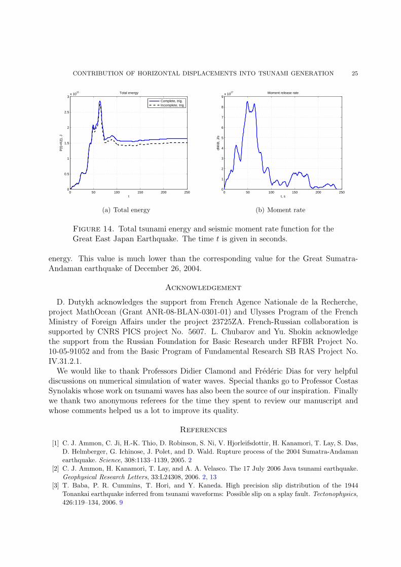
CONTRIBUTION OF HORIZONTAL DISPLACEMENTS INTO TSUNAMI GENERATION 25
0 50 100 150 200 2500
0.5
1
1.5
2
2.5
3x 10
15
t
P(t
)+K
(t),
J
Total energy
Complete, trig.Incomplete, trig.
(a) Total energy
0 50 100 150 200 2500
1
2
3
4
5
6
7
8
9x 10
27
t, s
dM/d
t, J/
s
Moment release rate
(b) Moment rate
Figure 14. Total tsunami energy and seismic moment rate function for theGreat East Japan Earthquake. The time t is given in seconds.
energy. This value is much lower than the corresponding value for the Great Sumatra-Andaman earthquake of December 26, 2004.
Acknowledgement
D. Dutykh acknowledges the support from French Agence Nationale de la Recherche,project MathOcean (Grant ANR-08-BLAN-0301-01) and Ulysses Program of the FrenchMinistry of Foreign Affairs under the project 23725ZA. French-Russian collaboration issupported by CNRS PICS project No. 5607. L. Chubarov and Yu. Shokin acknowledgethe support from the Russian Foundation for Basic Research under RFBR Project No.10-05-91052 and from the Basic Program of Fundamental Research SB RAS Project No.IV.31.2.1.
We would like to thank Professors Didier Clamond and Frederic Dias for very helpfuldiscussions on numerical simulation of water waves. Special thanks go to Professor CostasSynolakis whose work on tsunami waves has also been the source of our inspiration. Finallywe thank two anonymous referees for the time they spent to review our manuscript andwhose comments helped us a lot to improve its quality.
References
[1] C. J. Ammon, C. Ji, H.-K. Thio, D. Robinson, S. Ni, V. Hjorleifsdottir, H. Kanamori, T. Lay, S. Das,
D. Helmberger, G. Ichinose, J. Polet, and D. Wald. Rupture process of the 2004 Sumatra-Andaman
earthquake. Science, 308:1133–1139, 2005. 2
[2] C. J. Ammon, H. Kanamori, T. Lay, and A. A. Velasco. The 17 July 2006 Java tsunami earthquake.
Geophysical Research Letters, 33:L24308, 2006. 2, 13
[3] T. Baba, P. R. Cummins, T. Hori, and Y. Kaneda. High precision slip distribution of the 1944
Tonankai earthquake inferred from tsunami waveforms: Possible slip on a splay fault. Tectonophysics,
426:119–134, 2006. 9

26 D. DUTYKH, D. MITSOTAKIS, L. B. CHUBAROV, AND YU. I. SHOKIN
[4] J.-P. Bardet, C. E. Synolakis, H. L. Davies, F. Imamura, and E. A. Okal. Landslide Tsunamis: Recent
Findings and Research Directions. Pure Appl. Geophys., 160:1793–1809, 2003. 3
[5] C. Bassin, G. Laske, and G. Masters. The Current Limits of Resolution for Surface Wave Tomography
in North America. EOS Trans AGU, 81:F897, 2000. 5
[6] S. Beisel, L. Chubarov, I. Didenkulova, E. Kit, A. Levin, E. Pelinovsky, Yu. Shokin, and M. Sladkevich.
The 1956 Greek tsunami recorded at Yafo, Israel, and its numerical modeling. Journal of Geophysical
Research - Oceans, 114:C09002, 2009. 9
[7] E. Berg. Field survey of the Tsunamis of 28 March 1964 in Alaska, and conclusions as to the origin of
the major Tsunami. Technical report, Hawaii Institute of Geophysics, University of Hawaii, Honolulu,
1970. 3, 5
[8] R. Bilham. A flying start, then a slow slip. Science, 308:1126–1127, 2005. 2
[9] D. Clamond and D. Dutykh. Practical use of variational principles for modeling water waves. Physica
D: Nonlinear Phenomena, 241(1):25–36, 2012. 13
[10] R. R. Coifman and Y. Meyer. Nonlinear harmonic analysis and analytic dependence. Pseudodifferential
Operators and Applications, 43:71–78, 1985. 12
[11] W. Craig and C. Sulem. Numerical simulation of gravity waves. J. Comput. Phys., 108:73–83, 1993.
11, 12
[12] W. Craig, C. Sulem, and P.-L. Sulem. Nonlinear modulation of gravity waves: a rigorous approach.
Nonlinearity, 5(2):497–522, 1992. 11
[13] S. Das and P. Suhadolc. On the inverse problem for earthquake rupture: The Haskell-type source
model. Journal of Geophysical Research, 101(B3):5725–5738, 1996. 8
[14] A. I. Delis, M. Kazolea, and N. A. Kampanis. A robust high-resolution finite volume scheme for the
simulation of long waves over complex domains. Int. J. Numer. Meth. Fluids, 56:419–452, 2008. 4
[15] F. Dias and T. J. Bridges. The numerical computation of freely propagating time-dependent irrota-
tional water waves. Fluid Dynamics Research, 38:803–830, 2006. 11
[16] F. Dias and D. Dutykh. Dynamics of tsunami waves, chapter Dynamics o, pages 35–60. Springer,
2007. 4, 7, 10
[17] J. R. Dormand and P. J. Prince. A family of embedded Runge-Kutta formulae. J. Comp. Appl. Math.,
6:19–26, 1980. 14
[18] D. Dutykh. Mathematical modelling of tsunami waves. Ph.d. thesis, Ecole Normale Superieure de
Cachan, December 2007. 3, 7, 10
[19] D. Dutykh and F. Dias. Water waves generated by a moving bottom. In Anjan Kundu, editor, Tsunami
and Nonlinear waves, pages 65–96. Springer Verlag (Geo Sc.), 2007. 3, 5, 7, 8, 10
[20] D. Dutykh and F. Dias. Energy of tsunami waves generated by bottom motion. Proc. R. Soc. A,
465:725–744, 2009. 4, 12
[21] D. Dutykh and F. Dias. Tsunami generation by dynamic displacement of sea bed due to dip-slip
faulting. Mathematics and Computers in Simulation, 80(4):837–848, 2009. 3, 5
[22] D. Dutykh, F. Dias, and Y. Kervella. Linear theory of wave generation by a moving bottom. C. R.
Acad. Sci. Paris, Ser. I, 343:499–504, 2006. 8, 10, 16
[23] D. Dutykh, Th. Katsaounis, and D. Mitsotakis. Finite volume schemes for dispersive wave propagation
and runup. J. Comput. Phys, 230:3035–3061, 2011. 4
[24] D. Dutykh, D. Mitsotakis, X. Gardeil, and F. Dias. On the use of the finite fault solution for tsunami
generation problems. Theor. Comput. Fluid Dyn., March 2012. 4, 5, 6, 7, 12, 16, 22
[25] D. Dutykh, R. Poncet, and F. Dias. The VOLNA code for the numerical modeling of tsunami waves:
Generation, propagation and inundation. Eur. J. Mech. B/Fluids, 30(6):598–615, 2011. 3, 4
[26] H. M. Fritz, W. Kongko, A. Moore, B. McAdoo, J. Goff, C. Harbitz, B. Uslu, N. Kalligeris, D. Suteja,
K. Kalsum, V. V. Titov, A. Gusman, H. Latief, E. Santoso, S. Sujoko, D. Djulkarnaen, H. Sunendar,
and C. Synolakis. Extreme runup from the 17 July 2006 Java tsunami. Geophys. Res. Lett., 34:L12602,
2007. 2, 13, 23

CONTRIBUTION OF HORIZONTAL DISPLACEMENTS INTO TSUNAMI GENERATION 27
[27] D. Fructus, D. Clamond, O. Kristiansen, and J. Grue. An efficient model for threedimensional surface
wave simulations. Part I: Free space problems. J. Comput. Phys., 205:665–685, 2005. 11
[28] D. Fructus and J. Grue. An explicit method for the nonlinear interaction between water waves and
variable and moving bottom topography. J. Comp. Phys., 222:720–739, 2007. 5
[29] D. R. Fuhrman and P. A. Madsen. Tsunami generation, propagation, and run-up with a high-order
Boussinesq model. Coastal Engineering, 56(7):747–758, 2009. 5
[30] Y. Fujii and K. Satake. Source of the July 2006 West Java tsunami estimated from tide gauge records.
Geophys. Res. Lett., 33:L24317, 2006. 6
[31] E. Geist. Complex earthquake rupture and local tsunamis. J. Geophys. Res., 107:B5, 2002. 5
[32] E. L. Geist, S. L. Bilek, D. Arcas, and V. V. Titov. Differences in tsunami generation between the
December 26, 2004 and March 28, 2005 Sumatra earthquakes. Earth Planets Space, 58:185–193, 2006.
2, 5
[33] V. K. Gusiakov. Residual displacements on the surface of elastic half-space. In Conditionally correct
problems of mathematical physics in interpretation of geophysical observations, pages 23–51, 1978. 3
[34] P. Guyenne and D. P. Nicholls. A high-order spectral method for nonlinear water waves over moving
bottom topography. SIAM J. Sci. Comput., 30(1):81–101, 2007. 12
[35] J. Hammack. A note on tsunamis: their generation and propagation in an ocean of uniform depth. J.
Fluid Mech., 60:769–799, 1973. 8, 9, 16
[36] J. L. Hammack. Tsunamis - A Model of Their Generation and Propagation. PhD thesis, California
Institute of Technology, 1972. 8
[37] C. Harbitz. Model simulations of tsunamis generated by the Storegga Slides. Marine Geology, 104:1–
21, 1992. 3
[38] G. Hayes. Finite Fault Model Result of the Oct 25, 2010 Mw 7.7 Southern Sumatra Earthquake.
Technical report, USGS, 2010. 23
[39] G. Hayes. Finite Fault Model Result of the Mar 11, 2011 Mw 9.0 Earthquake Offshore Honshu, Japan.
Technical report, USGS, 2011. 24
[40] G. Ichinose, P. Somerville, H. K. Thio, R. Graves, and D. O’Connell. Rupture process of the 1964
Prince William Sound, Alaska, earthquake from the combined inversion of seismic, tsunami, and
geodetic data. Journal of Geophysical Research, 112(B7):B07306, July 2007. 6
[41] G. A. Ichinose, K. Satake, J. G. Anderson, and M. M. Lahren. The potential hazard from tsunami
and seiche waves generated by large earthquakes within Lake Tahoe, California-Nevada. Geophys.
Res. Lett., 27:1203–1206, 2000. 3
[42] F. Imamura. Long-wave runup models, chapter Simulation, pages 231–241. World Scientific, 1996. 4,
5
[43] F. Imamura, A. C. Yalciner, and G. Ozyurt. Tsunami modelling manual, April 2006. 5
[44] C. Ji. Preliminary Result of the 2006 July 17 Magnitude 7.7 - South of Java, Indonesia Earthquake.
Technical report, USGS, 2006. 6, 7, 8, 13
[45] C. Ji, D. J. Wald, and D. V. Helmberger. Source description of the 1999 Hector Mine, California
earthquake; Part I: Wavelet domain inversion theory and resolution analysis. Bull. Seism. Soc. Am.,
92(4):1192–1207, 2002. 5, 22
[46] J. M. Johnson and K. Satake. Source parameters of the 1957 Aleutian earthquake from tsunami
waveforms. Geophysical Research Letters, 20:1487–1490, 1993. 2
[47] K. Kajiura. The leading wave of tsunami. Bull. Earthquake Res. Inst., Tokyo Univ., 41:535–571, 1963.
2, 4
[48] K. Kajiura. Tsunami source, energy and the directivity of wave radiation. Bull. Earthquake Research
Institute, 48:835–869, 1970. 5
[49] H. Kanamori. The Alaska earthquake of 1964: Radiation of Long-Period Surface Waves and Source
Mechanism. Journal of Geophysical Research, 75(26):5029–5040, 1970. 2

28 D. DUTYKH, D. MITSOTAKIS, L. B. CHUBAROV, AND YU. I. SHOKIN
[50] H. Kanamori. Mechanism of tsunami earthquakes. Physics of the Earth and Planetary Interiors,
6(5):346–359, January 1972. 8
[51] H. Kanamori and L. Rivera. Energy partitioning during an earthquake.Geophysical Monograph Series,
170:3–13, 2006. 22
[52] Y. Kervella, D. Dutykh, and F. Dias. Comparison between three-dimensional linear and nonlinear
tsunami generation models. Theor. Comput. Fluid Dyn., 21:245–269, 2007. 5, 8, 10, 12, 16
[53] D.-H. Kim, Y.-S. Cho, and Y.-K. Yi. Propagation and run-up of nearshore tsunamis with HLLC
approximate Riemann solver. Ocean Engineering, 34:1164–1173, 2007. 4
[54] H. Lamb. Hydrodynamics. Cambridge University Press, 1932. 10
[55] J. F. Lander. Tsunamis affecting Alaska 1737 - 1996. U.S. Department of Commerce, National Oceanic
and Atmospheric Administration, 31:195, 1996. 2
[56] T. Lay, C. J. Ammon, H. Kanamori, Y. Yamazaki, K. F. Cheung, and A. R. Hutko. The 25 October
2010Mentawai tsunami earthquake (Mw 7.8) and the tsunami hazard presented by shallow megathrust
ruptures. Geophys. Res. Lett., 38:L06302, 2011. 23
[57] T. Lay, H. Kanamori, C. J. Ammon, M. Nettles, S. N. Ward, R. C. Aster, S. L. Beck, S. L. Bilek,
M. R. Brudzinski, R. Butler, H. R. DeShon, G. Ekstrom, K. Satake, and S. Sipkin. The great Sumatra-
Andaman earthquake of 26 December 2004. Science, 308:1127–1133, 2005. 2, 22
[58] F. Lø vholt, H. Bungum, C. B. Harbitz, S. Glimsdal, C. Lindholm, and G. Pedersen. Earthquake
related tsunami hazard along the western coast of Thailand. Nat. Hazards Earth Syst. Sci., 6:1–18,
2006. 22
[59] L. Mansinha and D. E. Smylie. Effect of earthquakes on the Chandler wobble and the secular polar
shift. J. Geophys. Res., 72:4731–4743, 1967. 3, 7
[60] L. Mansinha and D. E. Smylie. The displacement fields of inclined faults. Bull. Seism. Soc. Am.,
61:1433–1440, 1971. 3, 7
[61] J. McCloskey, A. Antonioli, A. Piatanesi, K. Sieh, S. Steacy, M. Nalbant S. Cocco, C. Giunchi, J. D.
Huang, and P. Dunlop. Tsunami threat in the Indian Ocean from a future megathrust earthquake
west of Sumatra. Earth and Planetary Science Letters, 265:61–81, 2008. 5
[62] C. C. Mei. The applied dynamics of ocean surface waves. World Scientific, 1994. 10
[63] R. D. Mindlin. Force at a point in the interior of a semi-infinite medium. Physics, 7:195–202, 1936. 7
[64] D. E. Mitsotakis. Boussinesq systems in two space dimensions over a variable bottom for the generation
and propagation of tsunami waves. Math. Comp. Simul., 80:860–873, 2009. 3, 16
[65] T. Ohmachi, H. Tsukiyama, and H. Matsumoto. Simulation of tsunami induced by dynamic displace-
ment of seabed due to seismic faulting. Bull. Seism. Soc. Am., 91:1898–1909, 2001. 3
[66] Y. Okada. Surface deformation due to shear and tensile faults in a half-space. Bull. Seism. Soc. Am.,
75:1135–1154, 1985. 3, 4, 7
[67] Y. Okada. Internal deformation due to shear and tensile faults in a half-space. Bull. Seism. Soc. Am.,
82:1018–1040, 1992. 3, 4, 7
[68] E. Okal and C. E. Synolakis. Field survey and numerical simulations: a theoretical comparison of
tsunamis from dislocations and landslides. Pure Appl. Geophys., 160:2177–2188, 2003. 2
[69] E. A. Okal and C. E. Synolakis. A theoretical comparison of tsunamis from dislocations and landslides.
Pure and Applied Geophysics, 160:2177–2188, 2003. 3
[70] A. Ozgun Konca. Preliminary Result 06/07/17 (Mw 7.9) , Southern Java Earthquake. Technical
report, http://www.tectonics.caltech.edu/slip history/2006, USGS, 2006. 6, 13, 19, 20, 23
[71] A. Piatanesi, S. Tinti, and G. Pagnoni. Tsunami waveform inversion by numerical finite-elements
Green’s functions. Nat. Hazards Earth Syst. Sci., 1:187–194, 2001. 6
[72] C. Pires and P. M. A. Miranda. Sensitivity of the adjoint method in the inversion of tsunami source
parameters. Nat. Hazards Earth Syst. Sci., 3:341–351, 2003. 6
[73] F. Press. Displacements, strains and tilts at tele-seismic distances. J. Geophys. Res., 70:2395–2412,
1965. 7

CONTRIBUTION OF HORIZONTAL DISPLACEMENTS INTO TSUNAMI GENERATION 29
[74] A. B. Rabinovich, L. I. Lobkovsky, I. V. Fine, R. E. Thomson, T. N. Ivelskaya, and E. A. Kulikov.
Near-source observations and modeling of the Kuril Islands tsunamis of 15 November 2006 and 13
January 2007. Adv. Geosci., 14:105–116, 2008. 3
[75] J. Rhie, D. Dreger, R. Burgmann, and B. Romanowicz. Slip of the 2004 Sumatra-Andaman Earthquake
from Joint Inversion of Long-Period Global Seismic Waveforms and GPS Static Offsets. Bulletin of
the Seismological Society of America, 97(1A):S115–S127, January 2007. 6
[76] T. Saito and T. Furumura. Three-dimensional tsunami generation simulation due to sea-bottom de-
formation and its interpretation based on the linear theory. Geophys. J. Int., 178:877–888, 2009. 3,
12, 16
[77] K. Satake. Linear and nonlinear computations of the 1992 Nicaragua earthquake tsunami. Pure Appl.
Geophys., 144(3-4):455–470, 1995. 12
[78] Y. T. Song, L.-L. Fu, V. Zlotnicki, C. Ji, V. Hjorleifsdottir, C. K. Shum, and Y. Yi. The role of
horizontal impulses of the faulting continental slope in generating the 26 December 2004 tsunami.
Ocean Modelling, 20:362–379, 2008. 3, 4, 5, 9
[79] Y. T. Song and T. Y. Hou. Parametric vertical coordinate formulation for multiscale, Boussinesq, and
non-Boussinesq ocean modeling. Ocean Modelling, 11(3-4):298–332, January 2006. 12
[80] J. A. Steketee. On Volterra’s dislocation in a semi-infinite elastic medium. Can. J. Phys., 36:192–205,
1958. 4, 7
[81] D. J. Stevenson. Tsunamis and Earthquakes: What Physics is interesting? Physics Today, June:10–11,
2005. 3
[82] J. J. Stoker. Water waves, the mathematical theory with applications. Wiley, 1958. 10
[83] C. E. Synolakis and E. N. Bernard. Tsunami science before and beyond Boxing Day 2004. Phil. Trans.
R. Soc. A, 364:2231–2265, 2006. 2, 4
[84] Y. Tanioka and K. Satake. Tsunami generation by horizontal displacement of ocean bottom. Geo-
physical Research Letters, 23:861–864, 1996. 3, 4, 5, 9, 12
[85] V. V. Titov and F. I. Gonzalez. Implementation and testing of the method of splitting tsunami
(MOST) model. Technical Report ERL PMEL-112, Pacific Marine Environmental Laboratory, NOAA,
1997. 5
[86] M. I. Todorovska, A. Hayir, and M. D. Trifunac. A note on tsunami amplitudes above submarine
slides and slumps. Soil Dynamics and Earthquake Engineering, 22:129–141, 2002. 8
[87] M. I. Todorovska and M. D. Trifunac. Generation of tsunamis by a slowly spreading uplift of the
seafloor. Soil Dynamics and Earthquake Engineering, 21:151–167, 2001. 5, 8
[88] Y. Tsuji, F. Imamura, H. Matsutomi, C. E. Synolakis, P. T. Nanang, Jumadi, S Harada, S. S. Han,
K. Arai, and B. Cook. Field survey of the East Java earthquake and tsunami of June 3, 1994. Pure
Appl. Geophys., 144:839–854, 1995. 2
[89] A. S. Velichko, S. F. Dotsenko, and E. N. Potetyunko. Amplitude-energy characteristics of tsunami
waves for various types of seismic sources generating them. Phys. Oceanogr., 12(6):308–322, 2002. 4
[90] A. Venkataraman and H. Kanamori. Observational constraints on the fracture energy of subduction
zone earthquakes. J. Geophys. Res., 109:B05302, 2004. 22
[91] J. K. Vennard and R. L. Street. Elementary fluid mechanics. Springer, sixth edition, 1982. 3, 4
[92] V. Volterra. Sur l’equilibre des corps elastiques multiplement connexes.Annales Scientifiques de l’Ecole
Normale Superieure, 24(3):401–517, 1907. 7
[93] K. T. Walker, M. Ishii, and P. M. Shrearer. Rupture details of the 28 March 2005 Sumatra Mw 8.6
earthquake imaged with teleseismic P waves. Geophysical Research Letters, 32:24303, 2005. 2
[94] X. Wang and P.L.-F. Liu. An analysis of 2004 Sumatra earthquake fault plane mechanisms and Indian
Ocean tsunami. J. Hydr. Res., 44(2):147–154, 2006. 5
[95] S. N. Ward. Landslide tsunami. J. Geophysical Res., 106:11201–11215, 2001. 3
[96] G. B. Whitham. Linear and nonlinear waves. John Wiley & Sons Inc., New York, 1999. 10, 20

30 D. DUTYKH, D. MITSOTAKIS, L. B. CHUBAROV, AND YU. I. SHOKIN
[97] Y. Yagi. Source rupture process of the 2003 Tokachi-oki earthquake determined by joint inversion of
teleseismic body wave and strong ground motion data. Earth Planets Space, 56(3):311–316, 2004. 6
[98] V. E. Zakharov. Stability of periodic waves of finite amplitude on the surface of a deep fluid. J. Appl.
Mech. Tech. Phys., 9:190–194, 1968. 11
LAMA, UMR 5127 CNRS, Universite de Savoie, Campus Scientifique, 73376 Le Bourget-
du-Lac Cedex, France
E-mail address : [email protected]
URL: http://www.lama.univ-savoie.fr/~dutykh/
IMA, University of Minnesota, 114 Lind Hall, 207 Church Street SE, Minneapolis MN
55455, USA
E-mail address : [email protected]
URL: http://sites.google.com/site/dmitsot/
Institute of Computational Technologies, Siberian Branch of the Russian Academy of
Sciences, 6 Acad. Lavrentjev Avenue, 630090 Novosibirsk, Russia
E-mail address : [email protected]
URL: http://www.ict.nsc.ru/
Institute of Computational Technologies, Siberian Branch of the Russian Academy of
Sciences, 6 Acad. Lavrentjev Avenue, 630090 Novosibirsk, Russia
E-mail address : [email protected]
URL: http://www.ict.nsc.ru/