HAL Id: halshs-01592863https://halshs.archives-ouvertes.fr/halshs-01592863

Preprint submitted on 25 Sep 2017

HAL is a multi-disciplinary open accessarchive for the deposit and dissemination of sci-entific research documents, whether they are pub-lished or not. The documents may come fromteaching and research institutions in France orabroad, or from public or private research centers.

L’archive ouverte pluridisciplinaire HAL, estdestinée au dépôt et à la diffusion de documentsscientifiques de niveau recherche, publiés ou non,émanant des établissements d’enseignement et derecherche français ou étrangers, des laboratoirespublics ou privés.

On the consistency of the two-step estimates of theMS-DFM: a Monte Carlo study

Catherine Doz, Anna Petronevich

To cite this version:Catherine Doz, Anna Petronevich. On the consistency of the two-step estimates of the MS-DFM: aMonte Carlo study. 2017. halshs-01592863

WORKING PAPER N° 2017 – 42

On the consistency of the two-step estimates of the MS-DFM: a Monte Carlo study

Catherine Doz Anna Petronevich

JEL Codes: Keywords: Markov-switching, Dynamic Factor models, two-step estimation, small-sample performance, consistency, Monte Carlo simulations

PARIS-JOURDAN SCIENCES ECONOMIQUES

48, BD JOURDAN – E.N.S. – 75014 PARIS TÉL. : 33(0) 1 43 13 63 00 – FAX : 33 (0) 1 43 13 63 10

www.pse.ens.fr

CENTRE NATIONAL DE LA RECHERCHE SCIENTIFIQUE – ECOLE DES HAUTES ETUDES EN SCIENCES SOCIALES

ÉCOLE DES PONTS PARISTECH – ECOLE NORMALE SUPÉRIEURE INSTITUT NATIONAL DE LA RECHERCHE AGRONOMIQUE – UNIVERSITE PARIS 1

On the consistency of the two-step estimates of the MS-DFM:a Monte Carlo studyI

Catherine Doza, Anna Petronevicha,b

aParis School of Economics, Universite Paris 1 Pantheon-Sorbonne

bCREST, Universita Ca’Foscari Venezia, NRU HSE

Abstract

The Markov-Switching Dynamic Factor Model (MS-DFM) has been used in different applications,notably in the business cycle analysis. When the cross-sectional dimension of data is high, theMaximum Likelihood estimation becomes unfeasible due to the excessive number of parameters.In this case, the MS-DFM can be estimated in two steps, which means that in the first step thecommon factor is extracted from a database of indicators, and in the second step the Markov-Switching autoregressive model is fit to this extracted factor. The validity of the two-step methodis conventionally accepted, although the asymptotic properties of the two-step estimates have notbeen studied yet. In this paper we examine their consistency as well as the small-sample behaviorwith the help of Monte Carlo simulations. Our results indicate that the two-step estimates areconsistent when the number of cross-section series and time observations is large, however, asexpected, the estimates and their standard errors tend to be biased in small samples.

Keywords: Markov-switching, Dynamic Factor models, two-step estimation, small-sampleperformance, consistency, Monte Carlo simulations

1. Introduction

Markov-Switching Dynamic Factor model (MS-DFM) has proved to be a useful instrument in anumber of applications. Among them are tracking of labor productivity (Dolega (2007)), modelingthe joint dynamics of the yield curve and the GDP (Chauvet and Senyuz (2012)), examination offluctuations in the employment rates (Juhn et al. (2002)) and many others. However, the majorapplication of the MS-DFM is the analysis of the business cycle turning points (see, for example,Kim and Yoo (1995), Darne and Ferrara (2011), Camacho et al. (2012), Chauvet and Yu (2006),Wang et al. (2009)). The initially suggested univariate Markov-switching model in the seminal pa-per by Hamilton (1989) was extended to the multivariate case, the MS-DFM, by Kim (1994). Themodel allows to obtain the turning points in a transparent and replicable way, and, importantly,

IThe authors are thankful to Monica Billio, Jean-Michel Zakoian, Christian Francq and the participants of theinternal Macro Seminar of the University Ca’Foscari Venezia for their fruitful suggestions. We also acknowledgefinancial support by the European Commission in the framework of the European Doctorate in Economics ErasmusMundus (EDEEM).

in a more timely manner than the official institutions (OECD and NBER, for example).

The MS-DFM formalizes the idea of Diebold and Rudebusch (1996) that the economic vari-ables comove and follow a pattern with alternating periods of growth and decline, this comovementessentially representing the business cycle. More precisely, the model assumes that the economicindicators have a factor structure, i.e. are driven by some common factor, which itself follows aMarkov-switching dynamics with two regimes.

Depending on the number of economic series under consideration, the model can be estimatedusing different techniques. The original paper by Kim (1994) as well as some of the followingapplications is based on just a few economic indicators so the parameters and the factor can beestimated simultaneously with Kalman filter and Maximum Likelihood. However, when the num-ber of series increases, convergence problems may arise and, besides, the estimation may becometime-consuming since the number of parameters expands proportionally to the number of series.In the same time, the use of many economic indicators is desirable in order to consider as much in-formation on the business cycle as possible. A natural solution to this trade-off between the size ofthe information set and the computational time is the the estimation of the Markov-Switching andDynamic Factor parts of the MS-DFM separately, i.e. in two steps. Attractive in terms of applica-bility and information treatment, the two-step estimation method has been used in several studies(see, for example, Chauvet and Senyuz (2012), Darne and Ferrara (2011), Bessec and Bouabdallah(2015), Brave and Butters (2010), Davig (2008), Paap et al. (2009)). This method implies thatthe factor is extracted1 on the first step, and then the classical univariate Markov-switching modela la Hamilton (1989) is fit to the estimated factor on the second step. The two-step procedure ismuch easier to implement2 and does not impose any restrictions on the number of series by default.

Previous studies show the importance of the number of cross-sections N and the number ofobservations T for the accuracy of estimates on each of the steps. Connor and Korajczyk (1986)proved the consistency of the principal components estimator ft (commonly used in the first step)for fixed T and N →∞ under general assumptions used by Chamberlain (1983) and Chamberlainand Rothschild (1983) for the definition of the approximate factor structure. Stock and Watson(2002) examined conditions for the rates of N and T under which ft can be treated as data forthe OLS regression. More precisely, they show that the performance of the PCA is very good evenwhen the sample-size and the number of series are relatively small, N = 100 and T = 100. Furtheron, Bai and Ng (2006) and Bai and Ng (2013) extended this result showing that, under a standardset of assumptions usually used in factor analysis, the ft can be treated as data in subsequentregressions when N →∞, T →∞ and N2/T →∞. As for the second step, Kiefer (1978), Francqand Roussignol (1997), Francq and Roussignol (1998), Krishnamurthy and Ryden (1998), Doucet al. (2004) and Douc et al. (2011) show that under particular conditions the maximum likelihoodestimators of an autoregressive model with Markov regimes are consistent. Francq and Roussignol(1997) also propose a gaussian maximum pseudo-likelihood estimator, Krishnamurthy and Ryden

1Different methods of factor extraction can be applied, Kalman filter (for a small number of series) and PCA arethe most common ones.

2The procedures for the estimation of the Markov-Switching models are installed in some econometric softwaresuch as Eviews, Stata. The corresponding packages exist for Matlab and R.

2

(1998) derived the conditions under which the MLE are asymptotically Gaussian.

Even though the consistency of the estimates of the factor on the first step and the consistencyof the ML estimates of the Markov-switching model on the second step has been already shown,it is not straightforward that the ML estimates of the Markov-switching model which is fit to theestimated (and not observed directly) factors are consistent. To the best of our knowledge, theconsistency of the two-step estimates has not been shown yet. It is not very surprising since theasymptotic properties of Markov-switching autoregressive models are rather complicated and aredifficult to derive analytically.

Another concern of the two-step approach are the small-sample properties of the estimates.Indeed, Hosmer (1973), Hamilton (1991) and Hamilton (1996) find that asymptotic approxima-tions of the sampling distribution of the MLE may be inadequate in small-sample cases. In theirMonte Carlo study, Psaradakis and Sola (1998) have shown that ”the performance of the MLE wasoften unsatisfactory even for sample sizes as large as 400”, pointing out the non-normality of theempirical distribution of the estimates and the bias that that takes place.

The purpose of this paper is thus twofold. First, we study the consistency of the two-step esti-mates, where the factor is estimated with PCA. Secondly, we would like to examine the behaviorof the estimates in small samples and identify the minimum N and T required to obtain estimateswith a reasonably small bias. In addition, we check whether the distribution of the two-step es-timates approaches normal (as is the case for the Maximum Likelihood estimates of an MS-AR)given the amount of data usually available in macroeconomic applications. In this paper, we studythe aforementioned questions with the help of Monte Carlo simulations. The analytic proof ofconsistency is being prepared in a companion paper to this work.

This paper thus contributes to the literature on the analysis of the two-step estimates of theMS-DFM. Previously, Camacho et al. (2015) studied the performance of the two-step estimateswhere the factor is extracted with a linear DFM on the first step. Their study focused on thequality of identification of states and was based on the use of a few series (N not higher than8). Having compared the two-step results to regular (one-step) Maximum Likelihood estimates,the authors showed that the two-step results diverge from the one-step ones when the commonfactor is extracted with the help of a linear DFM while the data-generating process is a nonlinearMS-DFM, although the difference decreases when N rises or when the data are less noisy.

The paper is organized as follows. Section 2 describes the MS-DFM model. Section 3 presentsthe two-step estimation technique. In section 4 we describe the design of the Monte Carlo experi-ment and discuss the simulation results. Section 5 concludes.

2. Markov-Switching Dynamic Factor Model

In the present paper, we take the basic specification of the MS-DFM for the business cycle asin the seminal paper by Kim and Yoo (1995), and we assume that the growth rate cycle of the

3

economic activity has only two regimes (or states), associated with its low and high levels. Theeconomic activity itself is represented by an unobservable factor, which summarizes the commondynamics of several observable variables. It is assumed that the switch between regimes happensinstantaneously, without any transition period (as is considered, for example, by STAR familymodels). This assumption can be motivated by the fact that the transition period before deepcrises is normally short enough to be omitted. For example, the growth rate of French GDP fellfrom 0.5% in the first quarter of 2008 to -0.51% in the second quarter of the same year, and furtherdown to -1.59% in the first quarter of 20093.

The model is thus decomposed into two equations, the first one defining the factor model,and the second one describing the Markov switching autoregressive model which is assumed forthe common factor. More precisely, in the first equation, each series of the information set isdecomposed into the sum of a common component (the common factor loads each of the observableseries with a specific weight) and an idiosyncratic component:

yt = λft + zt, (1)

where t = 1, ..., T , yt is a N × 1 vector of economic indicators, ft is a univariate common factor, ztis a N×1 vector of idiosyncratic components uncorrelated with ft at all leads and lags, λ is a N×1vector. In this equation all series are supposed to be stationary, so that some of the componentsof yt may be the first differences of the initially non stationary economic indicator.

The idiosyncratic components zit’s, i = 1, ..., N , are mutually uncorrelated at all leads and lags,and each of them follows an autoregressive process

ψi(L)zit = εit, (2)

where ψi(L) is a lag polynomial such that ψi(0) = 1, εit ∼ N (0, σ2i ) and cov(εit, εjt) = 0 for all i 6= j.

The second equation describes the behavior of the factor ft, which is supposed to follow anautoregressive Markov Switching process with constant transition probabilities4. In what follows,we consider that the change in regime affects only the level of the constant with the high levelcorresponding to the expansion state and the low level to the recession state:

ϕ(L)ft = βSt + ηt, (3)

where ηt ∼ i.i.d. N (0, 1), ϕ(L) is an autoregressive polynomial such that ϕ(0) = 1.

The switching mean is defined as:

3INSEE, France, Gross Domestic Product, Total, Contribution to Growth, Calendar Adjusted, Constant Prices,SA, Chained, Change P/P

4Kim and Yoo (1995) showed that, in the business cycle applications, although the assumption of the timedependent probabilities improves the quality of the model, the gain in terms of loglikelihood is not very large.

4

βSt = β0(1− St) + β1St, (4)

where St takes a value 0 when the economy is in expansion and 1 otherwise, so β0 > β1. St followsan ergodic Markov chain, i.e.

P (St = j|St−1 = i, St−2 = k, ...) = P (St = j|St−1 = i) = pij . (5)

As it is assumed that there are two states only, St switches states according to a 2 × 2 transition

probabilities matrix defined as

[p0 1− p0

1− p1 p1

], where

P (St = 0|St−1 = 0) = p0,

P (St = 1|St−1 = 1) = p1. (6)

There is no restriction on the duration of each state, and the states are defined point-wise, i.e. arecession period may last one period only.

The present framework can be generalized to the case of a higher number of states and/orto regime dependence in the other parameters of the model (the variance of the error term, thecoefficients of the autoregressive polynomial). In our study, we consider the simplest case with tworegimes and a switch in constant as in this specification it is easier to control the data generatingprocess. It is also often selected by information criteria in the empirical applications.

3. Two-step estimation method

The model presented above can be cast into the state-space form and estimated with Maxi-mum Likelihood. However, the estimation is complicated as the likelihood function has to takeinto account all possible paths of St, which is 2T , and the number of parameters to estimate growsproportionally to the number of series in yt. While the first issue can be solved with collapsingprocedure suggested by Kim (1994), the second problem makes the solution unfeasible for large N .This is computationally challenging, and there are several ways to solve this issue. The one thatwe consider in this paper is estimating the model in two steps, where on the first step the factor isextracted from the data yt, while on the second step the estimated factor is used as if it were thetrue factor in order to obtain the estimates of equation (3). More precisely, the procedure is thefollowing.

Step 1

The factor ft is extracted from a large database of economic indicators according to equation (1)without taking its Markov-Switching dynamics into account. In the present paper, we use princi-pal component analysis to compute an approximation ft of the true factor. Indeed, since (ft) is astationary process, as we have discussed in the introduction, under a mild set of assumptions, it

5

is consistently estimated by ft. The factor can be extracted with a different method, for example,using the two-step estimator suggested by Doz et al. (2011) or Quasi-Maximum Likelihood esti-mator by Doz et al. (2012).

If we denote by Σ = 1T y′y the empirical correlation matrix of y (where y is the standardized y), by

D the N ×N diagonal matrix of with the eigenvalues of Σ in decreasing order, by V the N ×Nmatrix of the unitary eigenvectors corresponding to D, then the matrix of the principal componentsF is defined as:

F = yV ,

and the corresponding matrix of loadings Λ is:

Λ = V ′,

The first column of the matrix F is then the estimate ft of the true factor ft, whereas the firstcolumn of Λ is the estimate λ.

Step 2

The parameters of the autoregressive Markov-Switching model described by equations (3) and (5)are estimated by maximum likelihood, with ft replaced by ft. This amounts to fit the univariatemodel of Hamilton (1989) to the estimated factor ft, which is taken as if it were an observedvariable:

ϕ(L)ft = βSt + ut, (7)

where ut ∼ N(0, σ2). Suppose that θ = (ϕ(L), ψ1(L), ..., ψN (L), λ1, ..., λN , σ21, ..., σ

2N , β0, β1, p0, p1, σ

2)′

is the vector of unknown parameters, g(·) is the Gaussian density function. The log-likelihood func-tion takes the following form:

LT (f , θ) = ln l(f1, f2, ..., fT , θ) =T∑t=1

ln g(ft|It−1, θ), (8)

where we denote f = (f1, ..., fT ) and It−1 = f1, ..., ft−1. The density

g(ft|It−1, θ) =1∑j=0

1∑i=0

g(ft, St = j, St−1 = i|It−1, θ), (9)

is computed using filtered probability P (St = j|It, θ) on the basis of Bayes’ theorem:

g(ft, St = j, St−1 = i|It−1, θ) = g(ft|St = j, St−1 = i, θ)× P (St = j, St−1 = i|It−1, θ), (10)

6

where

g(ft|St = j, St−1 = i, It−1, θ) = (2πσ2)−1/2exp

−1

2

(ϕ(L)ft − βSt)2

σ2

(11)

P (S = j, St−1 = i|It−1, θ) = P (St = j|St−1 = i, θ)× P (St−1 = i|It−1, θ), (12)

and

P (St = j|It, θ) =1∑i=0

P (S = j, St−1 = i|It, θ) (13)

P (St = j, St−1 = i|It, θ) =g(ft, St = j, St−1 = i|It−1, θ)

g(ft|It−1, θ)

=g(ft|St = j, St−1 = i, It−1, θ)× P (St = j, St−1 = i|It−1, θ)

g(ft|It−1, θ)(14)

The recursion is initialized with the steady state probability π of being in state j ∈ 0; 1 at timet = 0:

π = P (S0 = 1|I0, θ) =1− p0

2− p0 − p1, (15)

P (S0 = 0|I0, θ) = 1− P (S1 = 1|I0, θ) = 1− π. (16)

The two-step estimates θ(f) are obtained as the maximum of the likelihood function LT (f , θ) us-ing numerical optimization algorithms. Then, for θ(f) given, we can infer the associated filteredprobability P (St = j|It, θ)5 with formulas (9)-(14). Also, it is possible to compute the smoothedprobabilities of each state P (St = 1|IT , θ) using backward filtering (see Hamilton (1989)).

In the majority of studies on business cycle fluctuations analyzed with MS-DFM, the filtered prob-ability of recession is the main focus. Since it allows to have an estimate of the state at time t onthe basis of the information available up to the moment t, it is used for the purposes of nowcasting.The smoothed probabilities are often used to establish business cycle dating retrospectively on thebasis of the full information set, i.e. a posteriori. It is therefore important to verify if the two-stepestimates provide good quality of identification of states in terms of both filtered and smoothedprobability.

5To simplify notations, we denote θ = θ(f).

7

4. Monte Carlo simulations

We use Monte Carlo simulations to examine the consistency of the two-step estimates as wellas their small-sample properties. We first discuss the experimental design. The numerical resultsfollow.

4.1. Experimental setup

4.1.1. The DGP

The data generating process (DGP) used in simulations is described in equations (1)-(5). Weassume for simplicity that the order of ϕ(L) is one and the order of ψi(L) is zero, i = 1, ..., N .The autoregressive polynomials of higher order would complicate the control over the variance ofthe factor and the idiosyncratic components without changing the essence of the dynamics of theunderlying processes (unless it renders the dynamics nonstationary). The DGP is therefore:

yit = λift + εit, (17)

(1− ϕL)ft = βSt + ηt, (18)

βSt = β1St + β0(1− St) = β0 + (β1 − β0)St, (19)

P (St = 0|St−1 = 0) = p0,

P (St = 1|St−1 = 1) = p1, (20)

where i = 1, ..., N , t = 1, ..., T , ηt ∼ N(0, 1). The factor loadings λi are generated from a normaldistribution and are normalized to have a unit sum of squares, i.e. λi = γi√

γ′γ, γi ∼ N(0, 1).6

The idiosyncratic disturbance terms εit are cross-sectionally independent and have a Gaussiandistribution εit ∼ N(0, σ2i ). The state variable St is a Markov switching process with two statesSt ∈ 0; 1 (0 corresponds to expansion, and 1 to recession) and transition probability matrix(

p0 1− p01− p1 p1

).

We put the unconditional mean of the factor to zero, a classical assumption for the factormodels. Since ESt = π, this imposes a fixed relation between β0 and β1:

β1 = β0(1−1

π). (21)

4.1.2. The parameters of control

Intuitively, besides the size of N and T , there are four aspects of the dynamics of the DGPthat might affect the quality of the estimates of the MLE. These are:

1. The persistence of each regime. For a given sample size, a more persistent regime is betteridentified since it is activated during longer periods of time.

6The vector λ is unitary in order to provide the same scale to the generated factor and the estimated factorobtained by PCA with normalized loadings.

8

2. The noise-to-signal ratios si =σ2i

V (yit). When the data are less noisy, the estimate of the factor

is more precise.

3. The persistence of the autoregressive dynamics of the factor. Presumably, the closer theroot of the autoregressive polynomial is to one in absolute value, the more difficult it is todistinguish between the change in regime and the long-lasting effect of a shock in the errorterm.

4. The share of variance of the factor due to the switch. If most of the variance of the factor isgenerated by the error term ηt, the states are more difficult to identify.

Under the assumption that the unconditional mean of the factor is zero, it is possible to showthat (see Appendix for the details) that the unconditional variance of the true factor ft is:

V (ft) =1

1− ϕ2

(σ2 + β20

(1− p11− p0

)(1 + ϕ(p0 + p1 − 1)

1− ϕ(p0 + p1 − 1)

)). (22)

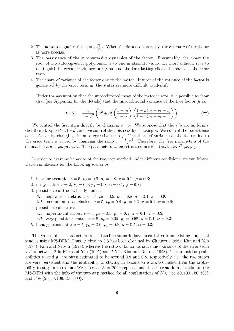
We control the first item directly by changing p0, p1. We suppose that the si’s are uniformlydistributed: si ∼ U [u; 1−u], and we control the noisiness by choosing u. We control the persistenceof the factor by changing the autoregressive term ϕ. The share of variance of the factor due tothe error term is varied by changing the ratio c = V (ft)

σ2 . Therefore, the free parameters of thesimulation are c, p0, p1, u, ϕ. The parameters to be estimated are θ = (β0, β1, ϕ, σ

2, p0, p1).

In order to examine behavior of the two-step method under different conditions, we run MonteCarlo simulations for the following scenarios:

1. baseline scenario: c = 5, p0 = 0.9, p1 = 0.8, u = 0.1, ϕ = 0.3;

2. noisy factor: c = 2, p0 = 0.9, p1 = 0.8, u = 0.1, ϕ = 0.3;

3. persistence of the factor dynamics:

3.1. high autocorrelation: c = 5, p0 = 0.9, p1 = 0.8, u = 0.1, ϕ = 0.9;3.2. medium autocorrelation: c = 5, p0 = 0.9, p1 = 0.8, u = 0.1, ϕ = 0.6;

4. persistence of states:

4.1. impersistent states: c = 5, p0 = 0.5, p1 = 0.5, u = 0.1, ϕ = 0.3;4.2. very persistent states: c = 5, p0 = 0.95, p1 = 0.95, u = 0.1, ϕ = 0.3;

5. homogeneous data: c = 5, p0 = 0.9, p1 = 0.8, u = 0.5, ϕ = 0.3;

The values of the parameters in the baseline scenario have been taken from existing empiricalstudies using MS-DFM. Thus, ϕ close to 0.3 has been obtained by Chauvet (1998), Kim and Yoo(1995), Kim and Nelson (1998), whereas the ratio of factor variance and variance of the error termvaries between 2 in Kim and Yoo (1995) and 7.5 in Kim and Nelson (1998). The transition prob-abilities p0 and p1 are often estimated to be around 0.9 and 0.8, respectively, i.e. the two statesare very persistent and the probability of staying in expansion is always higher than the proba-bility to stay in recession. We generate K = 2000 replications of each scenario and estimate theMS-DFM with the help of the two-step method for all combinations of N ∈ 25, 50, 100, 150, 300and T ∈ 25, 50, 100, 150, 300.

9

As the consistency properties of the PCA estimates have already been shown in previous liter-ature, we take as given that, with high values of N and T , we obtain a good estimate ft for thefactor ft in the first step. Interestingly, our simulations7 show that the factor can be estimatedwell even for N = 50 and T = 25, 50. In their Monte-Carlo study, Stock and Watson (2002)confirm this result.For this reason, we also report the behavior of the two-step estimates samplesas small as N = 25 and T = 25.8

4.1.3. Estimation

It is known that the PCA estimates of the factors are identified up to a sign change. We man-ually control the sign of the estimated factor by multiplying the f by -1 if its correlation with thetrue factor is negative. In practice, is it also usually possible to recover the sign of the true factor.

For each replication, the likelihood function LT (f , θ) is maximized under constraints on transi-tion probabilities (to insure that they lie in the open unit interval) and variance (to insure that it ispositive). The maximum likelihood estimate is obtained with SQP9 (sequential quadratic program-ming) method, which is essentially a version of Newton’s method for constrained optimization. Ateach iteration, the Hessian of the function is updated using the Broyden-Fletcher-Goldfarb-Shranno(BFGS) method. The variance-covariance matrix Ω−1T of the estimates θ(f) is then estimated as

ΩT = − 1

T

(∂2LT (θ, f)

∂θ∂θ′

)∣∣∣∣∣θ=θ

.

4.1.4. Measures of quality

In order to quantify the impact of the use of f instead of f on the ML estimates of the secondstep, we compare the empirical distributions of the two-step estimates to the MLE obtained on theobserved factor. We denote by θ(f) (resp. θ(f)) the vector estimates obtained with equation (3)(resp. equation (7)), and by θi(f) (resp. θi(f)) the i-th component of θ(f) (resp. θ(f)). For eachpair of elements θi(f) and θi(f), we compute two following measures:

1. the Kullback-Leibler divergence

DKL(Ff ||Ff ) =∑j

F if (j) lnF if(j)

F if (j),

where F if

and F if are the empirical cumulative distribution functions of θi(f) and θi(f), and

Ff (j) and Ff (j) are probability measures on a bin j.10 This is a measure of the information

7To save space, we do not report these results here, but they are surely available on request.8This setting may be interesting for the empirical studies of the business cycle in countries with limited availability

of data.9which corresponds to the sqp optimization algorithm of the fmincon optimizer in Matlab R2015a.

10In order to render the KL distances of the parameters comparable between each other, we set the width of a binto 0.25, the minimum value which guarantees non-emptiness of F if (j) for the distributions of each element of θi(f).

10

loss when F if

is used to approximate F if and corresponds to a proxy of the expectation of the

logarithmic difference.

2. the Kolmogorov-Smirnov statistic

KSi = supθi

|Ff (θi)− Ff (θi)|,

where supθi is the supremum of the set of distances between F if

and F if at different values

of θi. KSi shows the maximum deviation of Ff (θi) from Ff (θi). The statistic is used for

the Kolmogorov-Smirnov test with the null hypothesis that θi(f) and θi(f) come from thesame distribution. The null is rejected at 5% when KSi > 0.043.11 The KS statistic and thecorresponding test thus show whether the two empirical distributions are statistically differ-ent. It’s important to underline that the test requires that the two empirical distributionscorrespond to independent samples. For this reason, we compute Ff (θi) and Ff (θi) using

two disjoint subsets of 1000 replications, i.e. using the first 1000 replications for Ff (θi) and

the last 1000 replications for Ff (θi).

To study the small-sample behavior and consistency of the two-step estimates, we report the

ratio θi(f)θ0i

, where θ0i is the genuine value of the parameter, and the ratio between the mean esti-

mated standard error and sampling standard error of θi(f).

To measure the ability of the model to identify states we compare the obtained estimates offiltered probability P (St = 1|It) to the true sequence of states. To simplify notations, we useFPt(f) = P (St = 1|ft, ft−1, ..., f1) and FPt(f) = P (St = 1|ft, ft−1, ..., f1) for the filtered prob-ability corresponding to equations (7) and (3), respectively. We use the following quality indicators:

1. the quadratic probability score by Brier (1950), which measures the average quadratic devi-ation of the filtered probability from the true state and is defined as

QPS =1

T

T∑t=1

(St − FPt(f))2;

2. false positives score, which measures the average number of wrongly identified states in thesample, under the assumption that St = 1 when FPt(f) > 0.512 and St = 0 otherwise; FPSis defined as

FPS =1

T

T∑t=1

(St − IFPt(f)>0.5)2;

11In the general case, the null is rejected when KSn,n′ > c(α)√

n+n′nn′ where c(α) is the quantile of the Kolmogorov

distribution (c(α) = 1.36 for α = 0.05%), n and n′ are the sizes of first and second sample respectively.12The cut-off threshold of 0.5 for the filtered probability of recession is chosen arbitrary, however, it is quite common

in the literature.

11

3. the correlation between the true state and FPt(f)

r1 = corr(FPt(f), St);

4. the correlation between the true state and the filtered probability of recession inferred fromthe dynamics of the true factor

r2 = corr(FPt(f), St)

which allows to evaluate the performance of the Markov-Switching model for the identifica-tion of the state St in finite samples. By comparing r1 and r2, we can assess the impact ofthe use of the proxy of the factor ft instead of the factor ft itself.

While the correlations measure how well the filtered probability follows the business cycle, theQPS and FPS show how reliable it is about the estimate of the state and how often it fails. Thesame indicators QPS, FPS, r1 and r2 are computed for the smoothed probability of recession.

Finally, it is interesting to study whether the distribution of the two-step estimates has thesame properties as the MLE of the MS-AR model. Indeed, in case of a regular Markov-Switchingautoregressive model, is often assumed that under sufficient regularity conditions,13 the MLE θ isGaussian and so

√T (θ − θ0) converges in distribution to N(0,Ω−10 ) as T →∞, where

Ω0 = limT→∞

1

T

(∂2LT (f , θ)

∂θ∂θ′

)∣∣∣∣∣θ=θ0

,

and Ω0 is the information matrix.

In order to verify whether the two-step estimates have normal distribution (or tend to it asymp-totically), we study the conventional t-statistics corresponding to the elements of θi:

ti =θi(f)− θ0iσθi(f)

.

If the two-step estimates are asymptotically normal, the t-statistics should also have asymp-totically Gaussian distribution. In this case, the use of Wald-type tests (including significancetests) when interpreting the results of the MS-DFM is justified. We examine this hypothesis byanalyzing the mean, the skewness and the excess kurtosis of the distribution of ti, as well as run theKolmogorov-Smirnov normality test. As an additional indicator of gaussianity, we also computethe empirical rejection rates of the test with the null H0 : E(θi(f)) = θ0i. If the empirical rejectionrate coincides with the theoretical one, this is regarded as an additional sign of normality of thedistribution.

13see, for example, Kiefer (1978).

12

4.2. Simulation results

In this section we provide simulation results for the baseline scenario. The experiments wereperformed on SCSCF, a multiprocessor cluster system owned by Universita Ca’Foscari Venezia.

4.2.1. The impact of the first step

Figure 1 and Table 1 provide the information on how the first step - the use of estimated factorinstead of the true one - modifies the ML estimates of the Markov-Switching autoregressive model.For each matrix in Figure 1, the change in the color columnwise corresponds to the effect of theincrease of the number of series N , while the change rowwise to the increase of the number ofobservations T . As expected, the Kullback-Leibler distance between the empirical distributions ofθi(f) and θi(f) decreases when N rises. However, we observe the distance increase when T rises fora given N . This intuitively contradictory finding is connected to the presence of replications withaberrant results, i.e. replications with estimated transition probabilities very close to 0 or 1 (whichis an implausible result since it implies that the underlying Markov chain is not irreducible), orwith β0 is very close to β1 (in this case, the states are not identified, neither are the parameters). Inmost cases, these estimates correspond to the convergence of the maximum likelihood optimizer toa wrong local maximum. Present in both θ(f) and θ(f), this kind of estimates form an additionalmode which distorts the distributions. Since these obviously abnormal values of the estimators canbe easily identified as such while working with the real data, we discard them from our analysis.Typically, their amount is not large (5%-10% of replications, depending on the parameter), so theremaining number of replications is still large enough to analyze the properties of the two-stepestimator.14

Figure 2 reports the Kullback-Leibler divergence between θi(f) and θi(f) when the implausiblereplications are discarded. In this case we observe convergence both in N and T . Importantly,for all parameters the distance is high for N < 100. When N > 150, little improvement canbe achieved by increasing the number of series even more, so the major factor of proximity be-tween the two distributions is the number of observations. This observation is validated by theKolmogorov-Smirnov tests reported in Table 1, where the null that θi(f) and θi(f) come from thesame distribution is not rejected in the majority of cases.

14For the purpose of comparison, we compute several tables reported in this section for all replications (seeAppendix C). Other tables are available on request.

13

Figure 1: Kullback-Leibler distance between θi(f) and θi(f), with θ = (β0, β1, ϕ, σ2, p0, p1)

Figure 2: Kullback-Leibler distance between θi(f) and θi(f), with θ = (β0, β1, ϕ, σ2, p0, p1), aberrant replications

excluded

14

Table 1: Test statistic of the Kolmogorov-Smirnov test

N T β0 β1 ϕ σ2 p0 p1

25 25 0.05 0.07 0.08 0.10 0.04 0.0425 50 0.05 0.05 0.03 0.11 0.04 0.0425 100 0.08 0.07 0.06 0.14 0.05 0.0325 150 0.09 0.03 0.04 0.15 0.03 0.0425 300 0.09 0.03 0.07 0.15 0.04 0.0450 25 0.04 0.05 0.04 0.04 0.05 0.0650 50 0.03 0.06 0.03 0.10 0.04 0.0450 100 0.03 0.04 0.03 0.10 0.04 0.0450 150 0.07 0.06 0.06 0.09 0.06 0.0350 300 0.04 0.05 0.03 0.12 0.06 0.03100 25 0.06 0.03 0.04 0.05 0.04 0.05100 50 0.03 0.03 0.03 0.05 0.05 0.05100 100 0.03 0.06 0.03 0.04 0.04 0.04100 150 0.03 0.03 0.03 0.07 0.04 0.06100 300 0.03 0.03 0.03 0.08 0.04 0.04150 25 0.04 0.06 0.05 0.03 0.06 0.06150 50 0.07 0.02 0.03 0.03 0.05 0.06150 100 0.02 0.05 0.04 0.04 0.04 0.05150 150 0.03 0.03 0.03 0.04 0.06 0.03150 300 0.02 0.05 0.04 0.07 0.02 0.06300 25 0.03 0.05 0.05 0.02 0.06 0.05300 50 0.03 0.04 0.03 0.03 0.04 0.04300 100 0.03 0.03 0.02 0.06 0.04 0.04300 150 0.04 0.03 0.02 0.04 0.03 0.03300 300 0.04 0.03 0.03 0.04 0.03 0.04

The null hypothesis of the test is that θi(f) and θi(f), with θ = (β0, β1, ϕ, σ2, p0, p1), are from the same continuous distribution.The null is rejected when KS > 0.043. The cases when the null is not rejected are marked with bold font.

4.3. Consistency and small-sample performance of the two-step estimates θ(f)

4.3.1. Mean bias

Figure 3 provides the ratios of the two-step estimates θi(f) to the true values of the parametersθ0i averaged over replications (the exact values of the ratios are given in Table B.1 in Appendix),whereas B.1 sheds light on their distributions.

We observe that, as T and N rise, the ratio for all elements of θ(f) approaches one indicatingconsistency of the estimates. Interestingly, the convergence is achieved faster for the estimates ofthe parameters corresponding to the switch, i.e. β0, β1, p0 and p1, the deviation of the estimatesof transition probabilities being no more than 3% even for very small N and T . The estimates of ϕand σ2 require greater N and T to approach their true values (the deviation is around 2%-4% forand ϕ and is much higher for σ2). As expected, the rate of convergence is lower for the two-stepestimates in comparison to the estimates computed with the observed factor (see Table D.1 in theAppendix), the convergence of θ(f) is achieved at T = 150 already.

In case of small T and N , the estimated values of the parameters deviate from their true values.The bias is generally a decreasing function of the sample size and the number of series, and for mostdesign points is substantially different from zero. Consistent with Psaradakis and Sola (1998), theestimates of ϕ, p0, p1 and β1

15 are always downward biased, whereas the estimates of β0 and σ2

15In our setting, its true value is β1 = −2; the values above 1 in Table B.1 indicate that the average value of β1 is

15

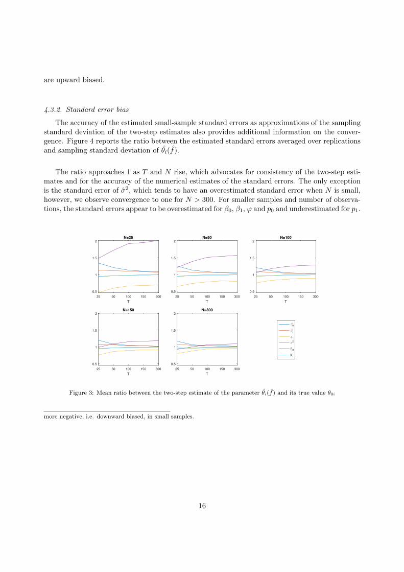
are upward biased.

4.3.2. Standard error bias

The accuracy of the estimated small-sample standard errors as approximations of the samplingstandard deviation of the two-step estimates also provides additional information on the conver-gence. Figure 4 reports the ratio between the estimated standard errors averaged over replicationsand sampling standard deviation of θi(f).

The ratio approaches 1 as T and N rise, which advocates for consistency of the two-step esti-mates and for the accuracy of the numerical estimates of the standard errors. The only exceptionis the standard error of σ2, which tends to have an overestimated standard error when N is small,however, we observe convergence to one for N > 300. For smaller samples and number of observa-tions, the standard errors appear to be overestimated for β0, β1, ϕ and p0 and underestimated for p1.

T

25 50 100 150 300

0.5

1

1.5

2N=25

T

25 50 100 150 300

0.5

1

1.5

2N=50

T

25 50 100 150 300

0.5

1

1.5

2N=100

T

25 50 100 150 300

0.5

1

1.5

2N=150

T

25 50 100 150 300

0.5

1

1.5

2N=300

β0

β1

φ

σ2

p0

p1

Figure 3: Mean ratio between the two-step estimate of the parameter θi(f) and its true value θ0i

more negative, i.e. downward biased, in small samples.

16

Figure 4: Ratio between mean estimated standard deviation σθi(f) and sample standard deviation of θi(f)

4.4. Identification of states

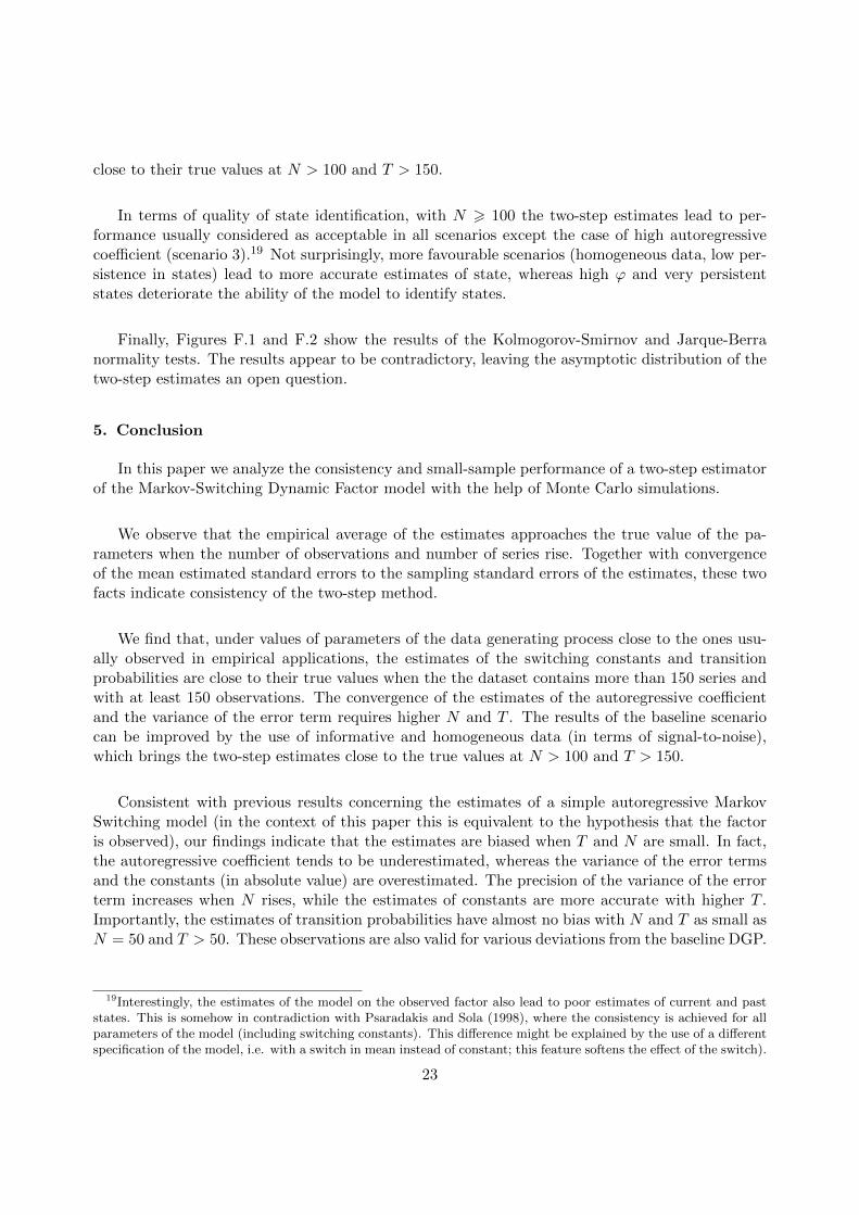
Figures 5 and 6 demonstrate the ability of the model to identify recession states.

As expected, the quality of state identification increases with the precision with which the fac-tor is estimated, and thus with the number of series N . In the same time, the factor reveals moreinformation about existing states when T is higher.

By comparing the sequence of filtered probabilities with the sequence of realized states we as-sess the quality of nowcasts of the current state of the cycle. Figure 5 shows that with T > 50 andN > 100, the model erroneously assigns a high probability of recession in at most 10% of cases(FPS < 0.10). In real empirical applications, the number of series that would produce the samequality should be lower, as the data are usually much less noisy (the results of scenario 4.1 confirmthis hypothesis). The correlation of the filtered probability of recession with the true states r1 isgetting closer to r2, its counterpart obtained with the observed factor, as N rises (up to almostcoinciding when N = 300) and is very high under values of N and T close to those usually used inpractice (above 0.8 for all T and N > 150).

The recession identification performance of the model is even higher for the retrospective anal-ysis of the cycles, i.e. for the smoothed probabilities. With T > 100 and N > 50, the FPS isbelow 0.10 and attains 0.03 with 300 observations on 300 series.

To conclude, it is worth noting that notwithstanding the bias in the two-step estimates when thenumber of series and observations are small, the two-step estimates seem to be precise enough toinsure high performance of the MS-DFM in terms of identification of states, especially a posteriori.

17

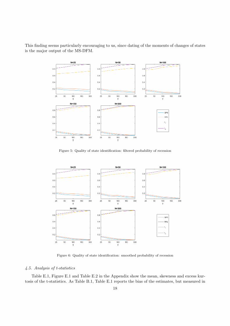
This finding seems particularly encouraging to us, since dating of the moments of changes of statesis the major output of the MS-DFM.

Figure 5: Quality of state identification: filtered probability of recession

Figure 6: Quality of state identification: smoothed probability of recession

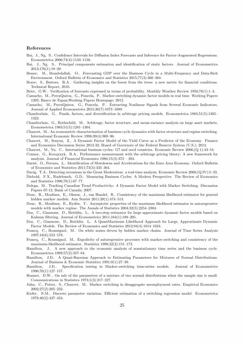
4.5. Analysis of t-statistics

Table E.1, Figure E.1 and Table E.2 in the Appendix show the mean, skewness and excess kur-tosis of the t-statistics. As Table B.1, Table E.1 reports the bias of the estimates, but measured in

18

standard deviations of the estimates. Once the standard deviations are accounted for, we observethat the bias of the estimates of p0 and p1 is very close to zero. The direction of bias of the t-statistics of the other estimates is in accordance with the results of Table B.1. One may notice thatthe values of the t-statistics in most design points is below 1.96 in absolute value, indicating that ifthe two-step estimates were asymptotically normal, the null H0 : E(θi) = θ0i would not be rejected.

For all values of N , the distribution of the t-statistics of the estimates are skewed, and skewnessoften changes sign when passing from small T to higher T and diminishes as N rises. Following thesign of the sample mean of the t-statistics, the skewness is negative for tϕ and tβ1 , and positive forthe other parameters. In particular, the empirical distribution of the two-step estimates of β0, β1and σ2 have thick right tails, whereas those of ϕ, p0 and p1 have thick left tails. The skewness of thetwo-step estimates of σ2, p0 and p1 is probably not very surprising since the estimation was imple-mented under the constraint that the variance should be positive and the transition probabilitiesshould lie in the open unit interval. These restrictions are likely to lead to finite-sample distri-butions resembling truncated ones, since more probability mass would lie in the required intervalthan would in a model with no restriction on the parameters. This effect is clearly visible on theboxplots of the ratio of the two-step estimates to their true values (see Figure B.1 in the Appendix).

Like the estimates obtained on the observed factors in small samples (see Psaradakis and Sola(1998)), the two-step estimates and their t-statistics are skewed and leptokurtic, at least in thesamples of size considered in this paper. We find nevertheless that in some cases the t-statistics areGaussian (see Figure F.1): the Kolmogorov-Smirnov test shows that normality of the distributionof tp1 is not rejected at 5% for all N and high T (and for small N and high T in case of tp0),however it is rejected for all other parameters. To the contrary, Jarque-Bera test does not rejectnormality for other parameters (see Figure F.2), so no unambiguous conclusion on the normalityof the two-step estimates can be derived.16

To get additional insight on the potential normality of the distribution of the two-step esti-mates, we analyze the empirical size of the tests of the null H0 : E(θi) = θ0i (see Tables E.3 andE.4). We observe that due to the distortions in the distributions, the empirical size of the testsis always above its the nominal size. As distortions attenuate, the empirical size gets closer to itsnominal counterpart, which we observe in case of β0, β1 (when the number of series and observa-tions is high) and, in particular, p0 and p1 (for N > 100). Consistent with Psaradakis and Sola(1998), the difficulties are the most serious for the t-statistics of σ2.

All the observations listed above lead us to the conclusion that the two-step estimates θ(f)17

are usually not normal for N < 300 and T < 300. This implies that the tests using this assumption(such as t-tests on significance of the coefficients, Wald-type tests, and other) are likely to be invalidand should be used with caution.

16Different normality tests are known to have different power depending on the shape of the distribution. Jarque-Bera is considered to be the most powerful when the distribution is symmetrical (i.e. in case of β0, β1 and ϕ), butit is overcome by Kolmogorov-Smirnov test in other cases (see Thadewald and Bning (2007) for details).

17as well as their counterpart θ(f), as reported by Psaradakis and Sola (1998).

19

4.6. Other scenarios

To analyze the behavior of two-step estimates under different parameter sets, we discuss theresults obtained with the other scenarios in terms of their deviation from the baseline scenario.Figures 7 and 8 show the ratio θi(f)

θ0iand the indicators of quality of state identification, allowing

us to compare the small-sample bias and the reliability of estimates of the current and past states.

20

Fig

ure

7:

Mea

nva

lues

of

two-s

tep

esti

mate

sfo

rdiff

eren

tsc

enari

os

β0

β1

φ

σ2

p0

p1

T=25

β0

β1

φ

σ2

p0

p1

T=50

β0

β1

φ

σ2

p0

p1

T=100

β0

β1

φ

σ2

p0

p1

T=150

β0

β1

φ

σ2

p0

p1

T=300

β0

β1

φ

σ2

p0

p1

β0

β1

φ

σ2

p0

p1

β0

β1

φ

σ2

p0

p1

β0

β1

φ

σ2

p0

p1

β0

β1

φ

σ2

p0

p1

β0

β1

φ

σ2

p0

p1

β0

β1

φ

σ2

p0

p1

β0

β1

φ

σ2

p0

p1

β0

β1

φ

σ2

p0

p1

β0

β1

φ

σ2

p0

p1

β0

β1

φ

σ2

p0

p1

β0

β1

φ

σ2

p0

p1

β0

β1

φ

σ2

p0

p1

β0

β1

φ

σ2

p0

p1

β0

β1

φ

σ2

p0

p1

β0

β1

φ

σ2

p0

p1

β0

β1

φ

σ2

p0

p1

β0

β1

φ

σ2

p0

p1

β0

β1

φ

σ2

p0

p1

β0

β1

φ

σ2

p0

p1

r<1

sce

na

rio

5sce

na

rio

4a

sce

na

rio

4sce

na

rio

3a

sce

na

rio

3scen

ario 2

sce

nario 1

N=25

N=50

N=100

N=150

N=300

a

aNote

:The

valu

eson

each

axis

variesfrom

0to

2,th

esh

aded

are

amark

ing

the

valu

esbelow

orequal1.

The

scenariosunderconsidera

tion

are

:sc

enario

1(b

ase

line

scenario):c

=5,p0

=0.9,

p1

=0.8,u

=0.1,ϕ

=0.3;sc

enario

2(n

oisy

facto

r):c=

2,p0

=0.9,p1

=0.8,u

=0.1,ϕ

=0.3;sc

enario

3.1

(high

auto

correlation):c=

5,p0

=0.9,p1

=0.8,u

=0.1,ϕ

=0.9;sc

enario

3.2

(mediu

mauto

correlation):c

=5,p0

=0.9,p1

=0.8,u

=0.1,ϕ

=0.6;sc

enario

4.1

(impersiste

ntstate

s):c

=5,p0

=0.5,p1

=0.5,u

=0.1,ϕ

=0.3;sc

enario

4.2

(very

persiste

ntstate

s):c

=5,p0

=0.95,

p1

=0.95,u

=0.1,ϕ

=0.3;sc

enario

5(h

omogeneousdata

):c=

5,p0

=0.9,p1

=0.8,u

=0.5,ϕ

=0.3

21

Figure 8: Indicators of quality of state identification for various scenarios, smoothed probability, N = 100

T

25 50 100 150 300

0

0.1

0.2

0.3

0.4

0.5

QPS

T

25 50 100 150 300

0

0.1

0.2

0.3

0.4

0.5

FPS

T

25 50 100 150 300

0

0.2

0.4

0.6

0.8

1

r1

T

25 50 100 150 300

0

0.2

0.4

0.6

0.8

1

r2

scenario 1 scenario 2 scenario 3 scenario 3a scenario 4 scenario 4a scenario 5

18

In spite of the fact that scenarios relate to very different conditions, we can track severalcommonalities:

• for small N and T , ϕ tends to be underestimated, whereas β0 and σ2 are overestimated;

• σ2 is estimated better when N rises; β0 and β1 are more accurate with higher T ;

• for all scenarios except scenario 3.1, the two-step estimates are very close to their true valuesfor N > 150 and T > 150;

• the two-step estimates of transition probabilities are the most accurate.

The differences between scenarios are clearly visible under small N and T . When the factoris noisy (scenario 2), the bias of the two-step estimates amplifies greatly for the autoregressivecoefficient and β0 and β1. When the factor dynamics has high persistence (ϕ is high, scenario3.1), the two-step method tends to confuse it with a large distance in mean, overestimating bothconstants to a large extent, and underestimating ϕ. The problem, however, disappears once thecharacteristic root is far enough from unity (scenario 3.2). The two-step method appears to beresistant to different degrees of persistence in states. For both low persistence and high persistencecases (scenario 4.1 and 4a, respectively), the distortions are comparable to the baseline scenario,being slightly higher in case of frequently changing regimes when N is low. The last scenario(homogeneous data) is, not surprisingly, the most favourable of all, bringing two-step estimates

22

close to their true values at N > 100 and T > 150.

In terms of quality of state identification, with N > 100 the two-step estimates lead to per-formance usually considered as acceptable in all scenarios except the case of high autoregressivecoefficient (scenario 3).19 Not surprisingly, more favourable scenarios (homogeneous data, low per-sistence in states) lead to more accurate estimates of state, whereas high ϕ and very persistentstates deteriorate the ability of the model to identify states.

Finally, Figures F.1 and F.2 show the results of the Kolmogorov-Smirnov and Jarque-Berranormality tests. The results appear to be contradictory, leaving the asymptotic distribution of thetwo-step estimates an open question.

5. Conclusion

In this paper we analyze the consistency and small-sample performance of a two-step estimatorof the Markov-Switching Dynamic Factor model with the help of Monte Carlo simulations.

We observe that the empirical average of the estimates approaches the true value of the pa-rameters when the number of observations and number of series rise. Together with convergenceof the mean estimated standard errors to the sampling standard errors of the estimates, these twofacts indicate consistency of the two-step method.

We find that, under values of parameters of the data generating process close to the ones usu-ally observed in empirical applications, the estimates of the switching constants and transitionprobabilities are close to their true values when the the dataset contains more than 150 series andwith at least 150 observations. The convergence of the estimates of the autoregressive coefficientand the variance of the error term requires higher N and T . The results of the baseline scenariocan be improved by the use of informative and homogeneous data (in terms of signal-to-noise),which brings the two-step estimates close to the true values at N > 100 and T > 150.

Consistent with previous results concerning the estimates of a simple autoregressive MarkovSwitching model (in the context of this paper this is equivalent to the hypothesis that the factoris observed), our findings indicate that the estimates are biased when T and N are small. In fact,the autoregressive coefficient tends to be underestimated, whereas the variance of the error termsand the constants (in absolute value) are overestimated. The precision of the variance of the errorterm increases when N rises, while the estimates of constants are more accurate with higher T .Importantly, the estimates of transition probabilities have almost no bias with N and T as small asN = 50 and T > 50. These observations are also valid for various deviations from the baseline DGP.

19Interestingly, the estimates of the model on the observed factor also lead to poor estimates of current and paststates. This is somehow in contradiction with Psaradakis and Sola (1998), where the consistency is achieved for allparameters of the model (including switching constants). This difference might be explained by the use of a differentspecification of the model, i.e. with a switch in mean instead of constant; this feature softens the effect of the switch).

23

When the baseline DGP is modified, we observe that the bias of the two-step estimates in-creases a lot for the autoregressive coefficient and the constants when the factor is noisier. Whenthe autoregressive coefficient is close to unity, the two-step method tends to confuse the effect ofhigh persistence in the dynamics with a large distance in mean, overestimating both constants toa large extent, and underestimating the autoregressive component. The problem, however, disap-pears once the characteristic root is far enough from unity. The two-step method appears to beresistant to different degrees of persistence in states. For both low persistence and high persistencecases the distortions are comparable to the baseline scenario, being slightly higher in case of fre-quently changing regimes when N is low.

In spite of the bias in small samples, the two-step estimates still lead to plausible state-detectionperformance of the MS-DFM with a dataset of dimensions commonly used in the business cycleanalysis (T > 100, N > 100), producing the filtered and smoothed probability of recession whichare highly correlated with the true underlying sequence of states and giving a reasonable amountof false recession signals.

The empirical distributions of the t-statistics associated to the two-step estimates in finitesamples tend to be skewed and leptokurtic and non-normal according to the Kolmogorov-Smirnovtest. Therefore, some of the traditional tests using the normality assumption (such as t-studentsignificance test or Wald-type test) are likely to be invalid. Similarly, the standard errors of theestimates should better be bootstrapped for small N and T . A positive exception are the param-eters of transition probabilities, which were found to be normally distributed when T > 300.

This paper shows the general validity of the two-step estimation method for small-samples. Itseems however likely that its performance can be improved by using more efficient estimates toestimate the factor on the first step. For example, the use of two-step method or Quasi-Maximumlikelihood estimates proposed by Doz et al. (2011) and Doz et al. (2012) for the first step mightprobably lead to more precise estimates in the second step.

24

References

Bai, J., Ng, S.. Confidence Intervals for Diffusion Index Forecasts and Inference for Factor-Augmented Regressions.Econometrica 2006;74(4):1133–1150.

Bai, J., Ng, S.. Principal components estimation and identification of static factors. Journal of Econometrics2013;176(1):18–29.

Bessec, M., Bouabdallah, O.. Forecasting GDP over the Business Cycle in a Multi-Frequency and Data-RichEnvironment. Oxford Bulletin of Economics and Statistics 2015;77(3):360–384.

Brave, S., Butters, R.A.. Gathering insights on the forest from the trees: a new metric for financial conditions.Technical Report; 2010.

Brier, G.W.. Verification of forecasts expressed in terms of probability. Monthly Weather Review 1950;78(1):1–3.Camacho, M., PerezQuiros, G., Poncela, P.. Markov-switching dynamic factor models in real time. Working Papers

1205; Banco de Espaa;Working Papers Homepage; 2012.Camacho, M., PerezQuiros, G., Poncela, P.. Extracting Nonlinear Signals from Several Economic Indicators.

Journal of Applied Econometrics 2015;30(7):1073–1089.Chamberlain, G.. Funds, factors, and diversification in arbitrage pricing models. Econometrica 1983;51(5):1305–

1323.Chamberlain, G., Rothschild, M.. Arbitrage, factor structure, and mean-variance analysis on large asset markets.

Econometrica 1983;51(5):1281–1304.Chauvet, M.. An econometric characterization of business cycle dynamics with factor structure and regime switching.

International Economic Review 1998;39(4):969–96.Chauvet, M., Senyuz, Z.. A Dynamic Factor Model of the Yield Curve as a Predictor of the Economy. Finance

and Economics Discussion Series 2012-32; Board of Governors of the Federal Reserve System (U.S.); 2012.Chauvet, M., Yu, C.. International business cycles: G7 and oecd countries. Economic Review 2006;(Q 1):43–54.Connor, G., Korajczyk, R.A.. Performance measurement with the arbitrage pricing theory: A new framework for

analysis. Journal of Financial Economics 1986;15(3):373 – 394.Darne, O., Ferrara, L.. Identification of Slowdowns and Accelerations for the Euro Area Economy. Oxford Bulletin

of Economics and Statistics 2011;73(3):335–364.Davig, T.A.. Detecting recessions in the Great Moderation: a real-time analysis. Economic Review 2008;(Q IV):5–33.Diebold, F.X., Rudebusch, G.D.. Measuring Business Cycles: A Modern Perspective. The Review of Economics

and Statistics 1996;78(1):67–77.Dolega, M.. Tracking Canadian Trend Productivity: A Dynamic Factor Model with Markov Switching. Discussion

Papers 07-12; Bank of Canada; 2007.Douc, R., Moulines, E., Olsson, J., van Handel, R.. Consistency of the maximum likelihood estimator for general

hidden markov models. Ann Statist 2011;39(1):474–513.Douc, R., Moulines, E., Ryden, T.. Asymptotic properties of the maximum likelihood estimator in autoregressive

models with markov regime. The Annals of Statistics 2004;32(5):2254–2304.Doz, C., Giannone, D., Reichlin, L.. A two-step estimator for large approximate dynamic factor models based on

Kalman filtering. Journal of Econometrics 2011;164(1):188–205.Doz, C., Giannone, D., Reichlin, L.. A QuasiMaximum Likelihood Approach for Large, Approximate Dynamic

Factor Models. The Review of Economics and Statistics 2012;94(4):1014–1024.Francq, C., Roussignol, M.. On white noises driven by hidden markov chains. Journal of Time Series Analysis

1997;18(6):553–578.Francq, C., Roussignol, M.. Ergodicity of autoregressive processes with markov-switching and consistency of the

maximum-likelihood estimator. Statistics 1998;32(2):151–173.Hamilton, J.. A new approach to the economic analysis of nonstationary time series and the business cycle.

Econometrica 1989;57(2):357–84.Hamilton, J.D.. A Quasi-Bayesian Approach to Estimating Parameters for Mixtures of Normal Distributions.

Journal of Business & Economic Statistics 1991;9(1):27–39.Hamilton, J.D.. Specification testing in Markov-switching time-series models. Journal of Econometrics

1996;70(1):127–157.Hosmer, D.W.. On mle of the parameters of a mixture of two normal distributions when the sample size is small.

Communications in Statistics 1973;1(3):217–227.Juhn, C., Potter, S., Chauvet, M.. Markov switching in disaggregate unemployment rates. Empirical Economics

2002;27(2):205–232.Kiefer, N.M.. Discrete parameter variation: Efficient estimation of a switching regression model. Econometrica

1978;46(2):427–434.

25

Kim, C.J.. Dynamic linear models with Markov-switching. Journal of Econometrics 1994;60(1-2):1–22.Kim, C.J., Nelson, C.R.. Business Cycle Turning Points, A New Coincident Index, And Tests Of Duration

Dependence Based On A Dynamic Factor Model With Regime Switching. The Review of Economics and Statistics1998;80(2):188–201.

Kim, M.J., Yoo, J.S.. New index of coincident indicators: A multivariate markov switching factor model approach.Journal of Monetary Economics 1995;36(3):607 – 630.

Krishnamurthy, V., Ryden, T.. Consistent estimation of linear and non-linear autoregressive models with markovregime. Journal of Time Series Analysis 1998;19(3):291–307.

Paap, R., Segers, R., van Dijk, D.. Do leading indicators lead peaks more than troughs? Journal of Business &Economic Statistics 2009;27(4):528–543.

Psaradakis, Z., Sola, M.. Finite-sample properties of the maximum likelihood estimator in autoregressive modelswith Markov switching. Journal of Econometrics 1998;86(2):369–386.

Stock, J., Watson, M.. Forecasting Using Principal Components From a Large Number of Predictors. Journal ofthe American Statistical Association 2002;97:1167–1179.

Thadewald, T., Bning, H.. Jarquebera test and its competitors for testing normality a power comparison. Journalof Applied Statistics 2007;34(1):87–105.

Wang, J.m., Gao, T.m., McNown, R.. Measuring Chinese business cycles with dynamic factor models. Journal ofAsian Economics 2009;20(2):89–97.

26

Appendix A. Variance of the factor

The formula for the variance of the factor is obtained in the following way.

V (ft) = V (βSt) + ϕ2V (ft−1) + V (ηt) + 2ϕCov(βSt , ft−1). (A.1)

The process (ft) is stationary, so

V (ft) =1

1− ϕ2[V (βSt) + V (ηt) + 2ϕCov(βSt , ft−1)] . (A.2)

Let us consider each part of V (ft) separately. The variance of the switching constant is:

V (βSt) = V (β0 + (β1 − β0)St)= (β1 − β0)2V (St)

= (β1 − β0)2(E(S2t )− E2(St))

= (β1 − β0)2(π − π2).

(A.3)

where E(St) = E(S2t ) = π.

The covariance term Cov(βSt , ft−1) is

Cov(βSt , ft−1) = Cov(βSt ,∞∑i=0

ϕiβSt−1−i +∞∑i=0

ϕiηSt−1−i)

= Cov(βSt ,∞∑i=0

ϕiβSt−1−i)

=∞∑i=0

ϕiCov(βSt , βSt−1−i)

= (β1 − β0)2∞∑i=0

ϕiCov(St, St−i−1),

(A.4)

where

Cov(St, St−i−1) = E(StSt−i−1)− E(St)E(St−i−1)

= E(StSt−i−1)− π2

=

1∑j=0

1∑k=0

jkP (St = j|St−i−1 = k)P (St−i−1 = k)− π2

= P (St = 1|St−i−1 = 1)π − π2.

(A.5)

27

If P (St|St−1) is the transition probability matrix for one time step:

P (St|St−1) =

(p0 1− p0

1− p1 p1

), (A.6)

and P (St|St−i−1) is the transition probability matrix for i time steps, then, according to Chapman-Kolmogorov theorem,

P (St|St−i−1) = (P (St|St−1))i+i. (A.7)

Using Cayley-Hamilton theorem or a diagonalization of this matrix, it can be shown that:

(p0 1− p0

1− p1 p1

)n=λ2λ

n1 − λ1λn2λ2 − λ1

I2 +λn2 − λn1λ2 − λ1

(p0 1− p0

1− p1 p1

), (A.8)

where λ1 and λ2 are the eigenvalues of the matrix

(p0 1− p0

1− p1 p1

), such that λ1 = 1,

λ2 = p0 + p1 − 1. So,

(p0 1− p0

1− p1 p1

)n=

1

p0 + p1 − 2

[(p0 − 1)(p0 + p1 − 1)n + p1 − 1 (1− p0)(p0 + p1 − 1)n + p0 − 1(1− p1)(p0 + p1 − 1)n + p1 − 1 (p1 − 1)(p0 + p1 − 1)n + p0 − 1

].

(A.9)

Therefore,

P (St = 1|St−i−1 = 1) = (P (St|St−1))i+i(2,2)

=1

p0 + p1 − 2

((p1 − 1)(p0 + p1 − 1)i+1 + p0 − 1

)= (1− π)(p0 + p1 − 1)i+1 + π.

(A.10)

Coming back to Cov(St, St−i−1):

Cov(St, St−i−1) = (1− π)π(p0 + p1 − 1)i+1 + π2 − π2

= (1− π)π(p0 + p1 − 1)i+1.(A.11)

Putting all terms together,

Cov(βSt , ft−1) =

∞∑i=0

ϕi(β1 − β0)2(1− π)π(p0 + p1 − 1)i+1

=(β1 − β0)2(1− π)π(p0 + p1 − 1)

1− ϕ(p0 + p1 − 1).

(A.12)

Finally,

28

V (ft) =1

1− ϕ2

[(β1 − β0)2(π − π2) + σ2 +

2ϕ(β1 − β0)2(π − π2)(p0 + p1 − 1)

1− ϕ(p0 + p1 − 1)

]=

1

1− ϕ2

[σ2 + (β1 − β0)2(π − π2)

1 + ϕ(p0 + p1 − 1)

1− ϕ(p0 + p1 − 1)

].

(A.13)

The nullity of the E(ft) implies that β1 = β0(1− 1π ), so the final expression for V (ft) becomes:

V (ft) =1

1− ϕ2

[σ2 + β20

(1− p11− p0

)(1 + ϕ(p0 + p1 − 1)

1− ϕ(p0 + p1 − 1)

)]. (A.14)

29

Appendix B. Two-step estimates distribution

Table B.1: Mean ratio between the two-step estimate of the parameter θi(f) and its true value θ0

N T β0/β0 β1/β1 ϕ/ϕ σ2/σ2 p0/p0 p1/p1

25 25 1.34 1.13 0.46 1.49 0.93 0.9525 50 1.21 1.12 0.60 1.72 0.96 0.9625 100 1.13 1.10 0.65 1.92 0.98 0.9725 150 1.10 1.08 0.67 1.95 0.99 0.9825 300 1.08 1.07 0.68 2.01 1.00 1.0050 25 1.25 1.10 0.65 1.20 0.93 0.9550 50 1.13 1.08 0.74 1.39 0.97 0.9750 100 1.08 1.07 0.77 1.51 0.99 0.9750 150 1.06 1.05 0.80 1.54 0.99 0.9950 300 1.05 1.05 0.80 1.57 1.00 1.00100 25 1.21 1.08 0.74 1.05 0.95 0.97100 50 1.12 1.06 0.82 1.17 0.97 0.96100 100 1.06 1.05 0.86 1.24 0.99 0.98100 150 1.04 1.04 0.89 1.26 0.99 0.98100 300 1.03 1.03 0.89 1.29 1.00 0.99150 25 1.20 1.08 0.76 0.98 0.95 0.96150 50 1.08 1.06 0.87 1.10 0.97 0.97150 100 1.04 1.04 0.90 1.15 0.99 0.98150 150 1.03 1.03 0.91 1.18 0.99 0.98150 300 1.02 1.02 0.92 1.19 1.00 0.99300 25 1.17 1.09 0.81 0.92 0.96 0.97300 50 1.07 1.05 0.89 1.01 0.98 0.97300 100 1.03 1.03 0.94 1.06 0.99 0.97300 150 1.03 1.02 0.94 1.08 0.99 0.98300 300 1.02 1.02 0.96 1.09 1.00 0.99

30

25

50

100

150

300

01234

beta

0, N

=25

25

50

100

150

300

0123

beta

0, N

=50

25

50

100

150

300

0123

beta

0, N

=100

25

50

100

150

300

0123

beta

0, N

=150

25

50

100

150

300

012

beta

0, N

=300

25

50

100

150

300

-202

ph

i, N

=25

25

50

100

150

300

024

ph

i, N

=50

25

50

100

150

300

-10123

ph

i, N

=100

25

50

100

150

300

-10123

ph

i, N

=150

25

50

100

150

300

-10123

ph

i, N

=300

25

50

100

150

300

05

10

sig

ma

2, N

=25

25

50

100

150

300

05

10

sig

ma

2, N

=50

25

50

100

150

300

123

sig

ma

2, N

=100

25

50

100

150

300

0123

sig

ma

2, N

=150

25

50

100

150

300

0.51

1.52

2.5

sig

ma

2, N

=300

25

50

100

150

300

0.6

0.81

p0, N

=25

25

50

100

150

300

0.6

0.81

p0, N

=50

25

50

100

150

300

0.6

0.81

p0, N

=100

25

50

100

150

300

0.6

0.81

p0, N

=150

25

50

100

150

300

0.6

0.81

p0, N

=300

25

50

100

150

300

0.6

0.81

1.2

p1, N

=25

25

50

100

150

300

0.6

0.81

1.2

p1, N

=50

25

50

100

150

300

0.6

0.81

1.2

p1, N

=100

25

50

100

150

300

0.6

0.81

1.2

p1, N

=150

25

50

100

150

300

0.6

0.81

1.2

ph

i, N

=300

Fig

ure

B.1

:Sam

ple

chara

cter

isti

csof

the

rati

oof

the

two-s

tep

esti

mate

sto

thei

rtr

ue

valu

es

31

Appendix C. Results on unfiltered data

Table C.1: Test statistic of the Kolmogorov-Smirnov test

N T β0 β1 ϕ σ2 p0 p1

25 25 0.04 0.11 0.08 0.07 0.20 0.0825 50 0.08 0.11 0.12 0.08 0.27 0.0925 100 0.10 0.16 0.18 0.12 0.37 0.1225 150 0.07 0.14 0.19 0.12 0.42 0.1825 300 0.12 0.22 0.16 0.15 0.44 0.3050 25 0.04 0.08 0.03 0.03 0.15 0.1050 50 0.04 0.08 0.07 0.08 0.14 0.0650 100 0.06 0.10 0.10 0.10 0.29 0.1150 150 0.12 0.15 0.11 0.12 0.32 0.1650 300 0.07 0.20 0.15 0.15 0.40 0.26100 25 0.06 0.06 0.03 0.06 0.11 0.08100 50 0.04 0.06 0.04 0.04 0.11 0.05100 100 0.03 0.04 0.07 0.03 0.10 0.09100 150 0.06 0.09 0.08 0.08 0.13 0.05100 300 0.06 0.11 0.10 0.10 0.20 0.16150 25 0.05 0.03 0.05 0.02 0.13 0.09150 50 0.06 0.04 0.04 0.02 0.08 0.05150 100 0.03 0.03 0.05 0.04 0.11 0.06150 150 0.05 0.06 0.07 0.05 0.14 0.04150 300 0.04 0.09 0.09 0.08 0.12 0.06300 25 0.05 0.03 0.04 0.02 0.05 0.07300 50 0.04 0.03 0.04 0.04 0.06 0.05300 100 0.03 0.04 0.04 0.05 0.06 0.05300 150 0.04 0.02 0.02 0.04 0.02 0.02300 300 0.08 0.06 0.07 0.06 0.10 0.06

The null hypothesis of the test is that θi(f) and θi(f), with θ = (β0, β1, ϕ, σ2, p0, p1), are from the same

continuous distribution. The null is rejected when KS > 0.043. The cases when the null is not rejected aremarked with bold font.

32

Table C.2: Mean ratio between the two-step estimate of the parameter θi(f) and its true value

N T β0/β0 β1/β1 ϕ/ϕ σ2/σ2 p0/p0 p1/p1

25 25 1.40 0.90 0.87 1.45 0.74 0.7225 50 1.20 0.93 1.05 1.94 0.77 0.7425 100 1.11 0.91 1.07 2.28 0.78 0.7925 150 1.06 0.92 1.04 2.37 0.81 0.8125 300 1.03 0.93 0.97 2.50 0.85 0.8450 25 1.27 0.90 1.00 1.18 0.78 0.7350 50 1.10 0.94 1.07 1.52 0.84 0.8150 100 1.05 0.93 1.06 1.72 0.86 0.8650 150 1.03 0.95 1.02 1.74 0.90 0.8950 300 1.01 0.99 0.98 1.77 0.93 0.91100 25 1.23 0.88 1.01 1.04 0.82 0.76100 50 1.08 0.91 1.12 1.26 0.85 0.82100 100 1.02 0.97 1.03 1.33 0.92 0.90100 150 1.01 0.98 1.01 1.36 0.95 0.94100 300 1.01 1.01 0.94 1.34 0.98 0.97150 25 1.22 0.88 0.98 0.97 0.83 0.78150 50 1.06 0.92 1.11 1.19 0.87 0.84150 100 1.02 0.96 1.04 1.23 0.92 0.92150 150 1.01 0.98 1.01 1.23 0.96 0.95150 300 1.01 1.01 0.96 1.22 0.99 0.98300 25 1.19 0.89 1.02 0.93 0.84 0.79300 50 1.04 0.93 1.08 1.09 0.90 0.86300 100 1.00 0.97 1.05 1.13 0.94 0.93300 150 1.01 0.99 1.00 1.11 0.97 0.96300 300 1.01 1.01 0.98 1.11 0.99 0.98

33

Appendix D. ML estimates obtained with the observable factor ft

Table D.1: Mean ratio between θi(f) and its true value θ0i

T β0/β0 β1/β1 ϕ/ϕ σ2/σ2 p0/p0 p1/p1

25 1.13 0.84 1.04 0.82 0.84 0.8050 1.03 0.92 1.08 0.96 0.91 0.87100 1.00 0.97 1.04 1.00 0.96 0.94150 1.00 0.98 1.03 1.00 0.98 0.96300 1.00 1.00 1.00 1.00 1.00 0.99

Figure D.1: Mean ratio between θi(f) and its true value θ0i

34

Appendix E. Properties of empirical distributions of t-statistics corresponding to thetwo-step estimates

Table E.1: Sample mean of the t-statistics corresponding to θ(f)

N T tβ0tβ1

tϕ tσ2 tp0 tp1

25 25 0.82 -0.35 -1.03 0.37 -0.24 0.0625 50 0.66 -0.50 -0.96 1.27 -0.05 0.0825 100 0.54 -0.57 -1.16 2.26 0.01 0.0525 150 0.56 -0.63 -1.34 2.90 0.09 0.0625 300 0.63 -0.75 -1.80 4.35 0.17 0.1450 25 0.70 -0.29 -0.66 -0.01 -0.25 0.0750 50 0.46 -0.37 -0.68 0.82 0.02 0.1350 100 0.45 -0.48 -0.82 1.64 0.04 0.0350 150 0.38 -0.47 -0.86 2.16 0.06 0.0750 300 0.43 -0.59 -1.22 3.30 0.16 0.12100 25 0.60 -0.25 -0.50 -0.35 -0.15 0.11100 50 0.50 -0.32 -0.48 0.32 -0.06 0.04100 100 0.34 -0.36 -0.54 0.93 0.07 0.06100 150 0.28 -0.37 -0.55 1.32 0.04 0.01100 300 0.31 -0.40 -0.75 2.12 0.10 0.00150 25 0.63 -0.24 -0.47 -0.56 -0.15 0.10150 50 0.34 -0.32 -0.37 0.11 -0.03 0.07150 100 0.28 -0.31 -0.40 0.58 0.04 0.06150 150 0.22 -0.28 -0.43 0.92 0.07 0.03150 300 0.24 -0.35 -0.56 1.54 0.13 0.03300 25 0.52 -0.31 -0.35 -0.75 -0.08 0.15300 50 0.32 -0.29 -0.31 -0.27 0.03 0.06300 100 0.19 -0.24 -0.25 0.18 0.02 -0.01300 150 0.24 -0.19 -0.28 0.38 0.06 0.01300 300 0.19 -0.23 -0.31 0.74 0.10 0.01

Figure E.1: Skewness of the t-statistics corresponding to the estimates θi(f) at different N and T

35

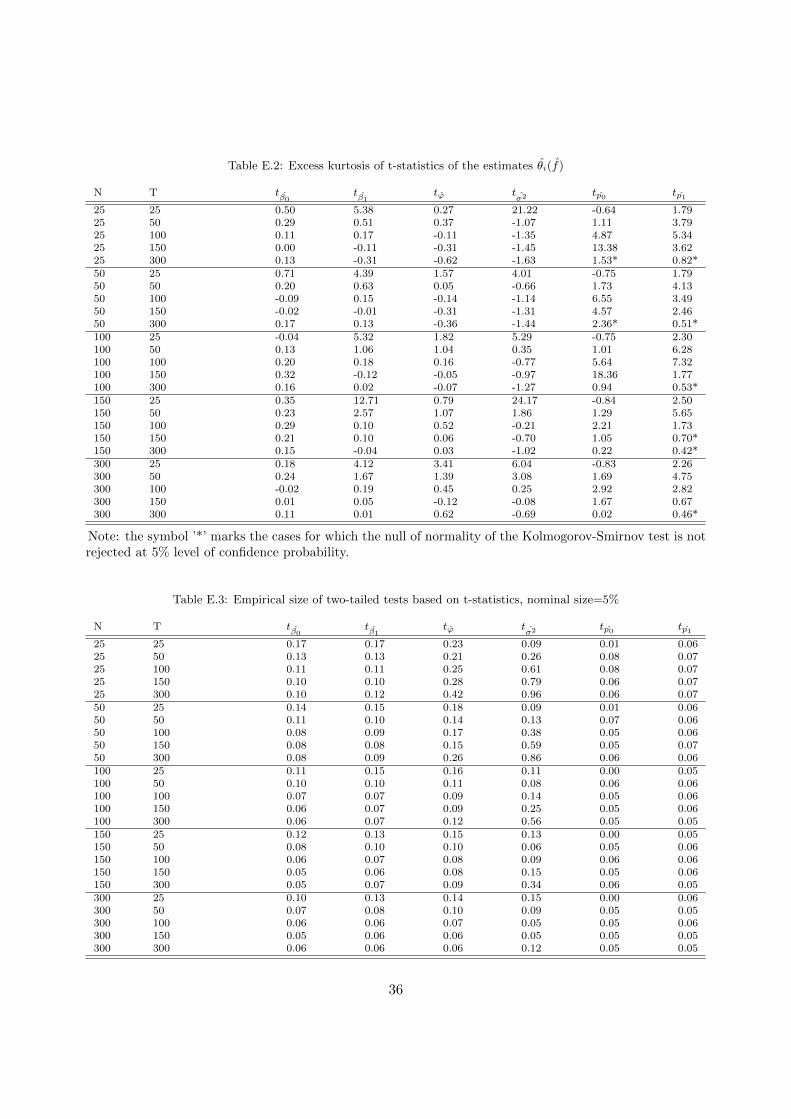
Table E.2: Excess kurtosis of t-statistics of the estimates θi(f)

N T tβ0tβ1

tϕ tσ2 tp0 tp1

25 25 0.50 5.38 0.27 21.22 -0.64 1.7925 50 0.29 0.51 0.37 -1.07 1.11 3.7925 100 0.11 0.17 -0.11 -1.35 4.87 5.3425 150 0.00 -0.11 -0.31 -1.45 13.38 3.6225 300 0.13 -0.31 -0.62 -1.63 1.53* 0.82*50 25 0.71 4.39 1.57 4.01 -0.75 1.7950 50 0.20 0.63 0.05 -0.66 1.73 4.1350 100 -0.09 0.15 -0.14 -1.14 6.55 3.4950 150 -0.02 -0.01 -0.31 -1.31 4.57 2.4650 300 0.17 0.13 -0.36 -1.44 2.36* 0.51*100 25 -0.04 5.32 1.82 5.29 -0.75 2.30100 50 0.13 1.06 1.04 0.35 1.01 6.28100 100 0.20 0.18 0.16 -0.77 5.64 7.32100 150 0.32 -0.12 -0.05 -0.97 18.36 1.77100 300 0.16 0.02 -0.07 -1.27 0.94 0.53*150 25 0.35 12.71 0.79 24.17 -0.84 2.50150 50 0.23 2.57 1.07 1.86 1.29 5.65150 100 0.29 0.10 0.52 -0.21 2.21 1.73150 150 0.21 0.10 0.06 -0.70 1.05 0.70*150 300 0.15 -0.04 0.03 -1.02 0.22 0.42*300 25 0.18 4.12 3.41 6.04 -0.83 2.26300 50 0.24 1.67 1.39 3.08 1.69 4.75300 100 -0.02 0.19 0.45 0.25 2.92 2.82300 150 0.01 0.05 -0.12 -0.08 1.67 0.67300 300 0.11 0.01 0.62 -0.69 0.02 0.46*

Note: the symbol ’*’ marks the cases for which the null of normality of the Kolmogorov-Smirnov test is notrejected at 5% level of confidence probability.

Table E.3: Empirical size of two-tailed tests based on t-statistics, nominal size=5%

N T tβ0tβ1

tϕ tσ2 tp0 tp1

25 25 0.17 0.17 0.23 0.09 0.01 0.0625 50 0.13 0.13 0.21 0.26 0.08 0.0725 100 0.11 0.11 0.25 0.61 0.08 0.0725 150 0.10 0.10 0.28 0.79 0.06 0.0725 300 0.10 0.12 0.42 0.96 0.06 0.0750 25 0.14 0.15 0.18 0.09 0.01 0.0650 50 0.11 0.10 0.14 0.13 0.07 0.0650 100 0.08 0.09 0.17 0.38 0.05 0.0650 150 0.08 0.08 0.15 0.59 0.05 0.0750 300 0.08 0.09 0.26 0.86 0.06 0.06100 25 0.11 0.15 0.16 0.11 0.00 0.05100 50 0.10 0.10 0.11 0.08 0.06 0.06100 100 0.07 0.07 0.09 0.14 0.05 0.06100 150 0.06 0.07 0.09 0.25 0.05 0.06100 300 0.06 0.07 0.12 0.56 0.05 0.05150 25 0.12 0.13 0.15 0.13 0.00 0.05150 50 0.08 0.10 0.10 0.06 0.05 0.06150 100 0.06 0.07 0.08 0.09 0.06 0.06150 150 0.05 0.06 0.08 0.15 0.05 0.06150 300 0.05 0.07 0.09 0.34 0.06 0.05300 25 0.10 0.13 0.14 0.15 0.00 0.06300 50 0.07 0.08 0.10 0.09 0.05 0.05300 100 0.06 0.06 0.07 0.05 0.05 0.06300 150 0.05 0.06 0.06 0.05 0.05 0.05300 300 0.06 0.06 0.06 0.12 0.05 0.05

36

Table E.4: Empirical size of two-tailed tests based on t-statistics, nominal size=10%

N T tβ0tβ1

tϕ tσ2 tp0 tp1

25 25 0.24 0.24 0.33 0.19 0.04 0.0825 50 0.20 0.21 0.31 0.38 0.13 0.1125 100 0.18 0.18 0.35 0.72 0.12 0.1225 150 0.17 0.18 0.38 0.86 0.11 0.1225 300 0.16 0.18 0.52 0.97 0.10 0.1150 25 0.20 0.24 0.26 0.15 0.03 0.0950 50 0.18 0.16 0.21 0.24 0.10 0.1050 100 0.13 0.15 0.24 0.52 0.10 0.1050 150 0.14 0.13 0.24 0.70 0.10 0.1150 300 0.13 0.17 0.36 0.91 0.11 0.11100 25 0.20 0.23 0.23 0.16 0.03 0.07100 50 0.17 0.17 0.18 0.14 0.09 0.09100 100 0.13 0.13 0.15 0.26 0.09 0.10100 150 0.11 0.14 0.17 0.38 0.10 0.11100 300 0.11 0.13 0.19 0.69 0.10 0.09150 25 0.20 0.21 0.23 0.17 0.03 0.08150 50 0.14 0.16 0.16 0.11 0.08 0.09150 100 0.11 0.13 0.13 0.17 0.11 0.11150 150 0.10 0.12 0.14 0.25 0.10 0.10150 300 0.10 0.13 0.16 0.47 0.11 0.10300 25 0.18 0.19 0.22 0.20 0.02 0.08300 50 0.13 0.15 0.16 0.14 0.09 0.09300 100 0.11 0.12 0.12 0.10 0.09 0.10300 150 0.10 0.11 0.13 0.11 0.09 0.09300 300 0.11 0.12 0.11 0.20 0.10 0.09

37

Appendix F. Simulations with various scenarios

Fig

ure

F.1

:R

esult

sof

the

Kolm

ogoro

v-S

mir

nov

norm

ality

test

for

the

t-st

ati

stic

sof

the

two-s

tep

esti

mato

rs,α

=5%

a

aN

ote

:ca

ses

when

the

hyp

oth

esis

isnot

reje

cted

are

mark

edin

gre

en.

38

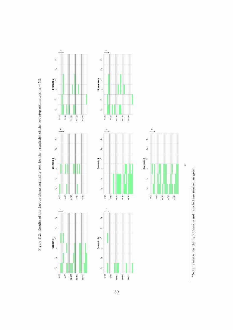
Fig

ure

F.2

:R

esult

sof

the

Jarq

ue-

Ber

ranorm

ality

test

for

the

t-st

ati

stic

sof

the

two-s

tep

esti

mato

rs,α

=5%

a

aN

ote

:ca

ses

when

the

hyp

oth

esis

isnot

reje

cted

are

mark

edin

gre

en.

39