on the consistency of bayes estimates author(s): persi

Institute of Mathematical Statistics is collaborating with JSTOR to digitize, preserve and extend access to The Annals of Statistics.

http://www.jstor.org

On the Consistency of Bayes Estimates Author(s): Persi Diaconis and David Freedman Source: The Annals of Statistics, Vol. 14, No. 1 (Mar., 1986), pp. 1-26Published by: Institute of Mathematical StatisticsStable URL: http://www.jstor.org/stable/2241255Accessed: 04-11-2015 02:06 UTC

Your use of the JSTOR archive indicates your acceptance of the Terms & Conditions of Use, available at http://www.jstor.org/page/ info/about/policies/terms.jsp

JSTOR is a not-for-profit service that helps scholars, researchers, and students discover, use, and build upon a wide range of content in a trusted digital archive. We use information technology and tools to increase productivity and facilitate new forms of scholarship. For more information about JSTOR, please contact [email protected].

This content downloaded from 128.173.127.127 on Wed, 04 Nov 2015 02:06:24 UTCAll use subject to JSTOR Terms and Conditions

http://www.jstor.org

http://www.jstor.org/action/showPublisher?publisherCode=ims

http://www.jstor.org/stable/2241255

http://www.jstor.org/page/info/about/policies/terms.jsp



The AnnaL'; of Statisttcs 1986, Vol. 14, No. 1, 1-26

SPECIAL INVITED PAPER ON THE CONSISTENCY OF BAYES ESTIMATES

BY PERSI DIACONIS1 AND DAVID FREEDMAN2

Stanford University and University of California, Berkeley We discuss frequency properties of Bayes rules, paying special attention

to consistency. Some new and fairly natural counterexamples are given, involving nonparametric estimates of location. Even the Dirichlet prior can lead to inconsistent estimates if used too aggressively. Finally, we discuss reasons for Bayesians to be interested in frequency properties of Bayes rules. As a part of the discussion we give a subjective equivalent to consistency and compute the derivative of the map taking priors to posteriors.

1. Consistency of Bayes rules. One of the basic problems in statistics can be put this way. Data is collected following a probability model with unknown parameters; the parameters are to be estimated from the data. Often, there is prior information about the parameters, for example, their probable sign or order of magnitude. Many statisticians express such information in the form of a prior probability over the unknown parameters. Estimates based on prior probabilities will be called Bayes estimates in what follows.

This paper studies points of contact between frequentist and Bayesian statistics. We derive frequency properties of Bayes estimates and suggest a Bayesian interpretation for some frequentist computations. Our main concern is consistency: as more and more data are collected, will the Bayes estimates converge to the true value for the parameters?

If the underlying probability mechanism has only a finite number of possible outcomes (tossing a coin or die) and the prior probability does not exclude the true parameter values as impossible, it has long been known that Bayes estimates are consistent. As will be discussed below, if the underlying mechanism allows an infinite number of possible outcomes (e.g., estimation of an unknown probability on the integers), Bayes estimates can be inconsistent: as more and more data comes in, some Bayesian statisticians will become more and more convinced of the wrong answer. The class of tail-free and Dirichlet priors was introduced to insure consistency in such settings. We present examples showing that mechanical extension of such priors to other very similar settings leads to inconsistent estimates.

In Section 2 we review other points of contact between the mathematics of frequentist and Bayesian statistics. In Section 3 we offer two Bayesian uses for

Received March 1984; revised August 1985. 'Research partially supported by National Science Foundation Grant MCS80-24649. 2Research partially supported by National Science Foundation Grant MCS83-01812. AMS 1980 subject classifications. 62A15, 62E20 Key words and phrases. Consistency, location problem, Dirichlet prior, merging of opinions,

foundations, uniformities.



2 P. DIACONIS AND D. FREEDMAN

frequentist computations. The first is a subjective equivalent to consistency involving intersubjective agreement. The second uses frequency computations as a way of thinking about priors. As part of the discussion, we compute the derivative of the map taking priors to posteriors. Mathematical details are given in the appendices.

To define things, consider a family of probabilities {Q6: 0 E)} on a space . Write Qa for the infinite product measure on .V0 which makes the coordinate random variables X1, X2,..., independent with common distribution Qo. We will assume throughout that ( and e are Borel subsets of complete separable metric spaces. Let M be a prior probability on e. Let P,, be the joint distribution of the parameter and the data:

P,(A x B) = AQ(B) (d)

for Borel sets A and B. The posterior is the P,-distribution of the parameter 0 given the data XI,..., X,; we denote this by Mn(d0IX1,..., X,,). The usual Bayes estimate is just the mean of the posterior.

Here are a few typical examples: Coin-tossing. .' has two points, H and T for heads and tails, respectively.

The parameter space E) can be taken as the unit interval: 0 - E) is the probability of a head. Then X is the space of sequences of heads and tails; Qx makes the sequence independent; in any position there is chance 0 of getting a head and 1 - 0 of getting a tail. We call this a "0-coin." Informally, P,i may be described as follows: choose 0 at random from ji, then toss a 0-coin. Of course, the posterior M n(dO X1,..., Xn) has a density with respect to the prior, proportional to the likelihood function:

OS(1 _ )n-S [JOS(, -_ )n-S(dO)]

where S is the number of heads and n - S the number of tails. Thus, the Bayes estimate is

JOS+1(l- _)n-SMi(d0)/f 0S(1 - 0)n-SM(dO).

Rolling a die. This is the same as coin tossing, except that -= (1, 2, 3, 4, 5, 6}, and e is the "6-simplex," all sequences 01,..., 06 of length six whose terms are nonnegative and add to one:

6

0. > 0 and 0. = 1. t=

Rolling an infinite die. The same, except X= {1,2,3,... } and E) is an infinite-dimensional simplex. Despite the superficial similarity, all the paradoxes of inconsistency already appear in this case. From our point of view, this is the simplest natural example of a nonparametric problem: estimating an unknown probability on the positive integers. On the other hand, we are still in the dominated case, so the posterior can still be computed in the usual way: lUn denotes this familiar version of the posterior.



CONSISTENCY OF BAYES ESTIMATES 3

The real line. Now X= (- oo, oo), and e is the set of all probabilities on 8. This is another nonparametric problem: estimating an unknown probability on the line. There is an additional complication: e is undominated. The posterior still exists but in general there is no explicit formula for it. There will usually be many versions of the posterior and this causes some technical difficulties.

We will use the weak-star topology: if ,in and , are probabilities on 9, then -Un *U iff ff dl4n J+ f dc for all bounded continuous functions f on 9. We

denote point mass at 6 by So. Thus, Ln -+ Se iff Jn(U) -+ 1 for every neighboar- hood U of 6.

In the coin tossing case, 03 is the unit interval; P ill weak-star if and only if Mn[O x] lX I 4O, x] for all intervals such that p{x} = 0. Turn next to the infinite die. Then pLn il li if and only if

tn(O101 < xl and 62 < X2... and 6k < Xk}

- L{681 < xl and 62 < X2... and Ok < Xk}

for all k and all x's such that

tl{6161= xl or 62 = X2 ... or ok = Xk} = .

Finally, take the line. Changing the imagery a little, Un ill if and only if

H Jfi(X) O(O)]n(d6) JH Jf1(x) I (dx) ](d)

for all k and all bounded continuous functions fi on X.

Consistency. The pair (6, O) iS consistent if for QOO-almost all sequences, the posterior ,ln converges to point mass at 6 in the weak-star topology. The weak-star topology has the fewest open sets of any natural topology, so it is fairly easy for posteriors to be consistent. Minor technical difficulties apart, if (6, un) iS consistent in our sense, the Bayes estimate for 0-in the sense of a posterior mean-will be consistent too. We say ,in iS conszstent if (6, ,in) iS consistent for all 6. Notice that consistency depends to some extent on the version selected for in-. Often, there is only one natural version, as in the dominated case. Sometimes, a natural version can be selected on the basis of continuity in the data: see Zabell (1979) and Tjur (1980). Sometimes, however, there is no sensible way to resolve the ambiguity. When there is a natural version of n, as in the dominated case, we will say that (6, .) is consistent rather than (6, I'r).

In the coin-tossing example, what does it mean for (6, lUn) to be consistent? Just that a Bayesian with prior ,u, who happens to be tossing a 6-coin, will eventually find this out: his posterior will concentrate in smaller and smaller intervals around 6 as more and more data comes in. Likewise for the infinite die. More specifically, (6, p) is consistent if and only if for any positive integer k and any small positive ,

tLn{NkeIXl1..., Xj -n 1 as n - oo a.e. Q0, where

Nke = f4: E e 9and lti - Oil < e for i = 1,..., k}.




For coin-tossing, (0, ,.) is consistent iff y assigns positive mass to every open interval around 0. For the infinite die the situation is much more complicated-and that is what the present discussion is all about.

Doob (1948) proved a very general theorem on consistency: one implication is that (0, ji,,) is consistent for M-almost all 0. Thus, a Bayesian with prior M can be sure that the posterior will converge. (This does not depend on the version, because null sets do not matter here.) Doob's work has been extended by Breiman, Le Cam, and Schwartz (1964). However, a frequentist using a Bayes rule will want to know for which O's the rule is consistent.

For smooth, finite-dimensional families, (0, tL) is consistent if and only if 0 is in the support of M. See Freedman (1963) or Schwartz (1965). (The support is the smallest closed set of probability 1.) But the assumption of finite dimensionality is really needed. For example, take X to be the positive integers. Take e to be the set of all probabilities on X. Take 0 to be the geometric distribution with parameter 4. Freedman (1963) constructed a prior M with the following properties:

* Every open neighborhood of 0 has positive n-probability. * For 0x-almost all sequences, the posterior converges to point mass at a

geometric distribution with parameter 3.

This example is generic in a topological sense: for most priors M and most parameters 0, the pair (0, tL) is inconsistent. To make this precise, we need the notion of "category." A set is of the first category if it is contained in a countable union of closed, nowhere dense sets. First-category sets are the topological equivalents of null sets. Put the weak-star topology on r(e), the set of priors on E. Then the set of consistent pairs (0, tL) is of the first category in e x r(e). See Freedman (1965).

Tail-free and Dirichlet priors. The existence of such counterexamples suggests the need for some careful investigation. Are there priors consistent for all parameters? (We will call such priors "consistent.") For countable X, Freedman suggested using tail-free and Dirichlet priors, showing that these priors are consistent at all parameters. This work was extended by Fabius (1964), who showed how to construct consistent tail-free priors for any complete, separable metric X. These ideas were further developed by Ferguson (1973,1974) with an excellent survey of the literature. Other extensions include "neutral-to-the-right priors." See Doksum (1974).

Here is a brief description of tail-free priors. For definiteness, consider the problem of estimating an unknown probability 0 on the positive integers. Write 0- for the ith coordinate of 0. We visualize the prior as randomly selecting a probability on the positive integers. Even more crudely, what the prior does is to randomly distribute a total mass of 1 among the integers. Thus, 01 is the randomly selected mass assigned to the integer 1, while 02 is the mass assigned to 2, and so on.




The simplest tail-free prior on the integers can be described by "stick-breaking." Let S1, S2,..., be independent and uniform over [0,1]. Think of a stick of unit length. Break off a piece of length 01 = Sl. This leaves a remaining piece of length 1 - 01. Now break off 02 = S2(1 - 01), 03 = S3(1 - 01 - 02), and so forth.

Freedman (1963) suggested a useful extension: the distribution of any finite number of the OA, say 1,. .., 0,N, can be specified in an essentially arbitrary way. Then the prior is completed by stick-breaking; the "cuts" Si are independent but not necessarily uniform or even identically distributed. The Si take values in (0, 1) and have arbitrary distributions with two restrictions: Si falls into any open interval with positive probability and 2E(Sj) = 00. The cuts are used to distribute mass inductively as follows: suppose mass m = ElN i0j < 1 has been assigned and mass 1 - m remains; now mass ON?1 = (1 - m)SN?l is assigned to N + 1 and mass

1 - m - (1 - m)SN+l = (1 - m)(1 - SN+1)

is left for the next move, which is carried out using SN +2, and so on. The motivation is as follows. A Bayesian may have a reasonably clear opinion

about Oi for some i's. However, it seems unlikely that such an opinion can be carefully quantified for all i. Freedman's extension of stick-breaking allows a Bayesian to approximate any prior by one consistent at all parameter values; indeed, any prior can be approximated (weak-star) by specifying the distribution of a finite number of Oi.

Early users of "stick-breaking" were Banach (1964), Kahane and Salem (1958), and Eberlein (1962). Kahane and Salem studied sums S = EL1riXi; the Xi are iid, taking the values 0 or 1 with probability 2 each; the ri are nonnegative and sum to 1. When is the distribution of S absolutely continuous? Kahane and Salem prove that for "almost all" sequences (rl, r2,... ) the law of S is absolutely continuous with an L2 density; "almost all" is relative to a stick-breaking measure. Banach and Eberlein were interested in a natural integral over the function spaces 12 and 11 and used stick-breaking as a key ingredient.

Dirichlet priors are tail-free; the Si having certain beta distributions. Usually, Dirichlet priors are parametrized in terms of a finite measure a on the observation space _, which is for the moment general. The Dirichlet prior D(a) with base measure a can be characterized as follows. Partition the observation space _ into a finite number of sets A1, A2,..., Ak. Consider a probability 0 on the observation space, selected at random from D(a). Then 0(A1),..., O(Ak) are random variables with respect to D(a). These have a Dirichlet distribution on the k-simplex, with parameter vector (a(A1),..., a(Ak)). More concretely, these are distributed like

UL/S, ... * Uk/S,

where S = U1 + * + Uk, the Ui being independent gamma variables with shape parameter a(Ai). When the observation space is the integers, a is specified by a countable collection of numbers a1, a2.. Let jjall = Eai. By assumption, all < 00. For a Dirichlet prior with parameter measure a on the positive




integers, the cut Si has a beta distribution with the two parameters al + * + a and Ilall - (a, + .. +aj).

Dirichlet priors have been suggested for use in a wide variety of problems. Also, some writers have considered using mixtures of Dirichlet priors; see Antoniak (1974) or Dalal and Hall (1980,1983). It is natural to ask whether mixtures of Dirichlet priors are consistent. The first step is easy; any mixture of a finite number of consistent priors is consistent. However, in Freedman and Diaconis (1983), we showed that a countable mixture of Dirichlet priors can be inconsistent. A starting point of our construction is an example showing that a mixture of a Dirichlet prior and a point mass at a certain long-tailed probability is inconsistent. Such priors are similar to the ones suggested by Jeffreys (1967) for Bayesian hypothesis testing. On the positive side, we showed that if the mass of the parameter measures are bounded, then the mixture is consistent.

The inconsistent priors in Freedman (1963) were constructed with malice aforethought. Bayesian reaction seems to be, "Oh, nobody would ever use a prior like that." See, for example, the remarks in Box, Leonard, and Wu (1983, page xi). That a Jeffreys-style prior is inconsistent should therefore be of interest. More- over, in Diaconis and Freedman (1986), we give examples of priors suggested by practicing Bayesians, which turn out to be inconsistent. That paper is fairly technical and the following heuristic discussion may be helpful.

The location problem. Consider estimating an unknown location parameter 0 with squared error as loss. The observations are modelled as

Xi = O + Ei, i = 1,2,....

The Ei are independent disturbance terms with a common distribution G. If G has known density g and a prior it is put on 0, then the Bayes estimate is the mean of the posterior distribution:

AfOH11g(xi -0) A(dO) (1.1) 0 f JH g(xi a-)) (dO)

If j((dO) is taken as Lebesgue measure, then this becomes the Pitman estimator. If the density g in (1.1) is unknown, it can be estimated from the data. Often, g is assumed to belong to some parametric family. Fraser (1976), Box and Tiao (1973, Chapters 3 and 4), and Johns (1979) all propose estimators of that general type, with a prior distribution on the parameters of the family. Such estimators can be inconsistent; the argument is like that in Freedman and Diaconis (1982b) or Diaconis and Freedman (1986) as outlined below.

A nonparametric approach to estimating G is also natural. This involves putting a prior on 0 and a prior on the law G of ij. Dalal (1979a, b) has suggested using a Dirichlet prior for G. We will now show that for a Dirichlet prior with a Cauchy base measure a, the Bayes estimates are inconsistent.

To avoid identifiability problems, we will assume that the law G of E is symmetric. To put a prior on symmetric G's, we symmetrize the Dirichlet as follows: if G is a distribution function for a random variable X, let G- be the distribution function of -X and let 0 = 1(G + G-), so 0 is symmetric. Let Da




be the law of G, where G has a Dirichlet distribution with base measure a on R. This is a symmetrized Dirichlet. The construction was first suggested by Dalal (1979a, b). For further discussion see Hannum and Hollander (1983). We assume that the base measure a has density a' and write IIaII = a(R). We make ) and G independent; our prior for 0 has density f on R while G is chosen from Da.

The posterior distribution of 0 is computed in Lemma 3.1 of Diaconis and Freedman (1986). For simplicity, we only discuss the Bayes estimate here.

THEOREM 1. Suppose that Xl,..., X,, are all distinct. Let Oij 1= (Xi + Xj) and suppose Oij are distinct. The Bayes estimate ( is

On = [@A(0) da + E aiji ]/l t( ) d i<} ]coi

with n

c(O) = jjajj f(O) H a'(Xk - 0), k=1

n

=i [ f2( )j )/(sij)] H a'(Xk Oij),

=ij (xi - Xj).

For the next result, take f to be standard nornal and a to be Cauchy. We suppose that in fact the Ei have a density h which is symmetric about 0, with a strict maximum at 0; further, h is infinitely differentiable and vanishes off a compact interval.

THEOREM 2. For some h, the Bayes estimate is inconsistent. Indeed, for large n, there is probability near 2 that On is close to y and probability near 1 that f9n is close to - y, where y # 0 depends on h.

REMARKS. (1) Theorem 2 is valid when a is any t-distribution. (2) When sampling from a continuous density, X' and 0 will be distinct with

probability 1. (3) The Bayes estimate 0 is a convex combination of two other estimates:

= fOw(0) dO/fw(0) dO

and

02= Eoij(1ij/ E ij i<j / i<j

The first is a Bayes estimate, as at (1.1), when sampling from known density a'. The second is a weighted average of the 0. ' which estimate 0 from the pair Xi and Xj. If a' is one of the standard unimodal densities such as normal or Cauchy, the weight wij is relatively large when Oij is in the center of the Xk's. It tums out




FIG. 1. The counterexample density h.

that 01 dominates 02 as n -x 00 for some h; for others 02 will dominate. Here, we focus on the first case.

(4) The h constructed in Theorem 2 is trimodal, as in Figure 1. It has a unique maximum at 0 but the two other modes matter. If desired, h can be chosen strictly positive on the interior of its interval of support.

(5) Any of the classical estimators, such as the mean or the median, will be consistent in this situation, so the Bayes estimates do worse than available frequentist procedures.

(6) In Diaconis and Freedman (1986), we argue that the Bayes estimate is consistent for any strongly unimodal density h: strong unimodality means that h increases up to its unique maximum and then decreases. Further, we show that if log a' is convex, then the Bayes estimate is consistent for any symmetric h.

(7) Doss (1983a, b, 1984) has carried out similar computations for neutral to the right and tail-free priors. He has also introduced some other methods of symmetrizing. Very roughly, his results parallel ours; it does not seem possible to find a consistent prior concentrated in a neighborhood of the normal location family.

(8) A subjective rationale for mixtures of location models is discussed in Freedman and Diaconis (1982a).

We now sketch the argument for inconsistency. As explained in Remark 3, the Bayes estimate is essentially

&l = f0 (0) dO@/|@() dO

with W(0) = Hi11/[1 + (Xi - 0)2], the Xi being the data. We have

)(0 ) = exp{t~E log[1 + (Xi - 0)2] )-exp{-nE[log(, + (X1 - 0)2)1>




FIG. 2. The function H.

In the approximation, the sum has been replaced by its mean under the true sampling distribution. Now consider

H(0) = E{log[1 + (X - 0)2]})

If X takes only the two values ? a where a > 1, then H has a local maximum at 0, a global minimum at + y, and tends to infinity at ? 00. Of course, H is symmetric. See Figure 2.

Now we estimate the integrals in the numerator and denominator of 01 by Laplace's method. As a function, ( 0) is close to exp[ - nH(0)], so only 0's near + matter, and as n tends to infinity, 01 oscillates between + -y and - y. The two-point distribution of X can be smoothed out to the density h shown in Figure 1.

This argument is like the one used in Freedman and Diaconis (1982b) to show inconsistency of M-estimators. It has been objected that the counterexample density h is not in the "support" of the Dirichlet, since the Dirichlet chooses a discrete measure with probability 1. A technical response is that the Dirichlet assigns positive mass to every open set of probabilities, so h is in the support-the smallest closed set of full prior mass. A broader response is that the Dirichlet assigns zero mass to any particular probability. After the fact, therefore, any troublesome probability can be differentiated in some qualitative way from a Borel set of full prior mass.

The foregoing discussion has all been asymptotic. WVhat are the implications with finite samples? Consider an estimation problem with a large amount of data -and a large number of parameters. A Bayes rule will do well for most parameter values, "most" being defined relative to the prior measure itself. On the other hand, a set of parameters which is large as judged by one measure may be quite small as judged by another, so Bayes rules may be quite unsatisfactory for a practical frequentist. Bayesians usually argue that the data will swamp the prior-but this may not happen in high-dimensional inference problems, or it may occur, but very slowly. Our view is that the oscillation at infinity will even show up with large, finite samples-in high-dimensional problems.




On the other hand, even the most dedicated subjectivist will usually not insist on quantifying all the precise details of a prior opinion in a high-dimensional situation. Our results indicate that small changes in the details of a prior can lead to Bayes rules with much better operating characteristics.

Quantifying these ideas is hard and that is why we give asymptotic results. We hope to study the finite-sample problem elsewhere, and in particular, we hope to quantify the extent to which small changes in the prior can make small changes in the posterior but big improvements in rates of convergence. The derivative of the posterior with respect to the prior is a relevant concept and will be discussed in Section 3.

2. Other connections between Bayesians and frequentists. Frequentists often discuss Bayes rules for the following reasons. First, the complete class theorem, as in Wald (1950), Le Cam (1955), Stein (1955), Sacks (1963), or Brown (1981), implies that all admissible procedures are approximately Bayes. Similarly, all minimax procedures are approximately Bayes. So not much is lost by confin- ing attention to Bayes procedures. Thus, Bayes procedures are convenient, tractable, and close to optimal. For instance, in some problems confidence sets are difficult to obtain. Welch and Peers (1963), Hinkley (1980), and Stein (1981) suggest using regions of high posterior mass, the prior being chosen so that Bayesian and frequentist coverage probabilities agree to several terms in an asymptotic expansion. Similarly, Bayesian techniques are used as a way of eliminating nuisance parameters. Berk (1970) gives examples of this in sequential analysis.

The common thread is a kind of pragmatic use of Bayes methods by frequentists: theory and convenience suggest the use of Bayes rules. As long as a Bayes rule is to be used, one may as well work with a prior that concentrates on a plausible part of the parameter space.

Second, Bayesian techniques can be helpful in proving frequentist theorems. For example, consider estimating the mean of a univariate normal with known scale and squared error loss. Any admissible estimator must be an analytic function of the observations. The only available proof uses complete class theorems of Sacks (1963) and Stein (1955) to represent the estimator as a formal Bayes rule. It is easy to show that formal Bayes rules are suitably smooth. Another example of this sort is in Matthes and Truax (1967).

Naturally, frequentists have been interested in frequentist properties of Bayes procedures. Theorems dating back to Laplace (1774) show that the posterior distribution can be approximated by the distribution of the maximum likelihood estimator. Modem versions of these theorems can be found in Bernstein (1934), Von Mises (1964), Johnson (1967,1970), Le Cam (1982), or Ghosh et al. (1982). Bayesians use these results to show that standard frequentist procedures are nearly Bayes. See Lindley (1965).

There are many other points of contact between the frequentist and Bayesian schools. However, there is often some incompatibility between Bayes rules and frequentist desiderata. For example, Blackwell and Girschick (1954) followed by Blackwell and Bickel (1967) and Noorbaloochi and Meedan (1983) have shown




that there are essentially no unbiased Bayes procedures. Other points of difference are emphasized in survey articles by Pratt (1965), Cornfield (1969), Lindley (1972), and Neyman (1977). Savage (1972) gives a review.

Sufficiency gives a point of technical contact. Kolmogorov (1942) introduced the notion of Bayesian sufficiency-a statistic is Bayes sufficient if for any prior the posterior only depends on the data through the sufficient statistic. For smooth, finite-dimensional problems, Bayesian sufficiency is the same as the frequentist concept. Recently, Blackwell and Ramamoorthi (1982) give an infinite-dimensional example where the two notions disagree.

Points of agreement arise in Bayesian discussions of robustness as in Berger (1984) or Kadane and Chuang (1978). Here frequentist properties of Bayes procedures are used as a means of protection from naive specification of the prior. A similar compromise was suggested by Hodges and Lehmann (1952).

3. Bayesian interpretations of consistency. It is useful to separate Bayes- ians into two groups: we will call them "classical" and "subjectivist." Classical Bayesians, like Laplace or Bayes himself, seemed to believe there is a true but unknown parameter which is to be estimated from data. This parameter is part of an objective probability model for the data. Prior opinion about the parameter is expressed as a probability distribution. Subjective Bayesians like de Finetti and Savage reject such ideas; for them, probabilities represent degrees of belief and there are no objective probability models. (Freedman used to be a classical Bayesian, while Diaconis is a subjectivist.)

Consistency properties of Bayes rules are clearly of interest to classical Bayesians; as data comes in, the posterior should converge to point mass at the true parameter. We will now argue that frequency properties of Bayes rules are also of interest to subjectivists. The first reason has to do with "intersubjective agreement." In some circumstances, Bayesians learn from experience, so opinions based on very different priors will merge as data accumulates; the data swamps the prior. We will now argue that consistency is equivalent to merging of intersubjective opinions under certain conditions.

A general result of this type was provided by Blackwell and Dubins (1962). To state their result, assume that P and Q are probabilities governing a process (X1, X2,... ). Let Pn and Qn be regular conditional probabilities for the future (Xn+1, Xn+2,...) given the past (X1, X2,..., Xn). We think of P and Q as the priors of two Bayesians, and assume P and Q are mutually absolutely continuous: P Q, the Bayesians agree on what is possible or impossible. Blackwell and Dubins show that almost surely, Pn and Qn merge in variation distance.

Reverting to the context of Section 1, assume that 0 -- Q6 is a homeomorphism and consider two Bayesians with priors ,u and v, respectively. Now ,u- v if and only if P, PI, and ,u l v if and only if P, I Pp. So the Blackwell-Dubins result does not apply when ,u l v, as is usually the case with Dirichlet priors. However, even if merging in variation distance does not happen, "weak-star merging" is still a possibility. We say two sequences {an}, {fi3} of probabilities merge weak-star if and only if an and fin become indistinguishable from the point of view of integrating bounded continuous functions: more precisely,




R(a z,/) 0 for every weak-star continuous function R defined on pairs of probabilities satisfying R(a, a) = 0. As an example, R might be a metric for weak-star convergence; or R(a, /P) might be ff da - ff d/3.

We show that the version pn is consistent if and only if P1 and P, merge weak-star for any v, in the following sense. Recall that P,, is the joint distribution of O and X1, X2 Let P be the law of + given X1,...,lX, determined by the formula

P,Un= IQ@?IJn (dO).

A Bayesian with prior ,u holds the opinion P,,, about the future X,+ 1, Xn+2. after seeing the data X1,..., Xn.

THEOREM 3. Suppose 0 -- Po is continuous, one-to-one, and continuously invertible. Suppose the version yn is consistent. Let v be any other prior. As n -x oo, P,n and Pn merge weak-star along P,,-almost all sequences. Conversely, if Pun and Pvn merge for all v, then yn is consistent.

Informally, the prior IL is consistent if and only if any other subjectivist with prior v is sure that P,4 and P, will merge on the future, as more and more data comes in. Theorem 3 is proved in Appendix A. Similar issues were considered by Lockett (1971).

This completes our discussion of "intersubjective agreement." We turn to our second reason for thinking that frequency properties should interest subjectivists as a way of specifying priors. The idea is simple: after specifying a prior distribution, generate imaginary data sequences, compute the posterior, and consider whether the posterior would be an adequate representation of the updated prior. This is quite close to the checks for coherence proposed by de Finetti and Savage; see de Finetti (1974, pages 229-246) for examples and Savage (1971) for a review. This use of fictitious samples was suggested by the "device of imaginary results;" Good (1950, page 35) uses this device as a method of roughly quantifying a prior in difficult situations. We call it the "what if" method: what if the data came out that way?

Take the prior suggested by Dalal (1979b) for use in symmetric location problems as discussed in Section 1. If data were generated from the density h of Theorem 2, the posterior would oscillate and never converge to the center of symmetry. The " what if" method strongly suggests modifying the prior. We give further examples and discussion in Diaconis and Freedman (1983).

The "what if" method suggests various interesting mathematical problems. For example, to what extent do the Bayes estimates deteimine the prior? Diaconis and Ylvisaker (1979) show that the posterior mean of the natural parameter in an exponential family determines the prior under suitable regularity conditions. Diaconis and Ylvisaker (1985) give counterexamples in location problems.

For a fixed observation x, Bayes theorem gives the relationship between the posterior and the prior. This defines a map from measures to measures. In the




next theorem we calculate the derivative of this map and the norn of the derivative. This helps to identify data sets x where small changes in the prior cause large changes in the posterior. These may be the most informative x's for the " what if" method. (Of course, they may also be unlikely x 's.)

In the theorem, probabilities are considered as a subset of all signed measures, with distance defined by the variation norn: the distance between ,i and v is the total mass of the signed measure ,I - v. Equivalently,

d4L dp iitL-vii =f|j - du,

where a is any dominating a-finite measure, e.g., a = ,I + v. With this norm, the measures form a Banach space.

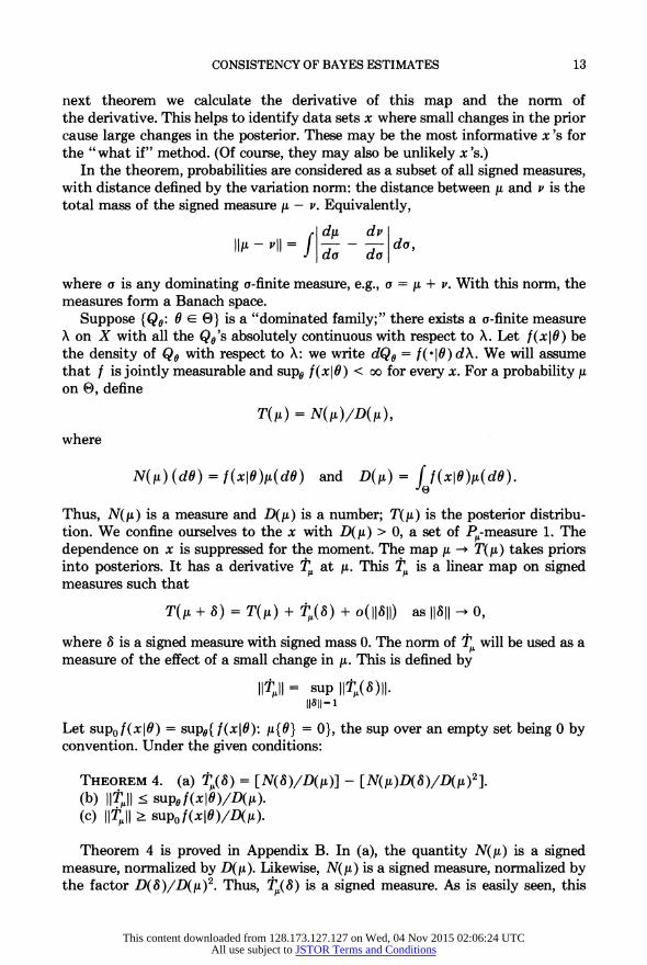
Suppose {Q6: 0 E 0) is a "dominated family;" there exists a a-finite measure X on X with all the Q6's absolutely continuous with respect to X. Let f(x I) be the density of Q6 with respect to X: we write dQ6 = f(-I0) dX. We will assume that f is jointly measurable and sup6 f(x IO) < o for every x. For a probability ,u on (, define

T(M) = N(I)ID(I), where

N(M) (dO) = f (x10)(dO) and D(y) = ff(xIO)A(dO).

Thus, N(M) is a measure and D(yi) is a number; T(1i) is the posterior distribution. We confine ourselves to the x with D(y) > 0, a set of P-measure 1. The dependence on x is suppressed for the moment. The map ,u-- T(,u) takes priors into posteriors. It has a derivative T, at ,. This T, is a linear map on signed measures such that

T(L + 8) = T(M) + Tu(S) + o(11811) as 11811 0,

where 8 is a signed measure with signed mass 0. The norm of T. will be used as a measure of the effect of a small change in ,. This is defined by

T11I = sup IIT1(8)II1 11i11= 1

Let supof(x I) = supe {f(xI0): It{0} = O}, the sup over an empty set being 0 by convention. Under the given conditions:

THEOREM 4. (a) T,(8) = [N(3)/D(M)] - [N(1)D(8)1D(1)']. (b) ITt < supo f (x I )ID(p). (c) IT, II supo f (x I )ID(pl).

Theorem 4 is proved in Appendix B. In (a), the quantity N(M) is a signed measure, normalized by D(y). Likewise, N(M) is a signed measure, nomalized by the factor D(3)/D(M)2. Thus, T1(8) is a signed measure. As is easily seen, this




measure has signed mass 0. For many priors the upper and lower bounds of (b) and (c) coincide. Then conclusion (b) has a simple interpretation in terms of likelihood ratios: the x's where the posterior is most sensitive to small changes in the prior are the x's which have high ratio of objectivist likelihood to subjectivist likelihood. These x's are the ones where the "what if" method will be most informative: at such x, small changes in the prior can make big changes in the posterior.

As an example, consider a nornal location problem with known variance a Without loss, suppose there is only one observation. Let ,i be a normal prior for the location parameter 0. Suppose that 1i has mean 1,0 and variance ao . Then D(y) at x turns out to be the nornal density at x with mean 110 and variance Ua2 + a 2. The norm computed in (b) is

[(a2 + a)/g 2]l/2exp{ (x - tL)2/(U2 + 2)

This is large when x is far from 110. We have carried out similar computations for the other standard one-dimensional exponential families with conjugate priors. The results are similar: values of x far from the mean of the prior lead to large norms.

On the other hand, for examples of the type considered in Freedman and Diaconis (1983), the posterior concentrates at some distance from the maximum likelihood estimate, so ff d11 will be many orders of magnitude smaller than max f for most data sets, relative to the true sampling distribution. Such data sets will have high leverage, and a posterior, which may seem on reflection to be unsatisfactory, so the " what if" method might prompt revision of an inconsistent prior. This completes our discussion of the "what if" method and with it Bayesian defense of frequentist analysis.

4. Conclusion. We return now to the big picture. There is a probability model for data and some of the parameters are to be estimated. A statistician who really has a sharp prior probability distribution for these parameters should use it, according to Bayes theorem; inconsistency on a null set of a priori probability zero is an irrelevant nuisance. On this point, there seems to be general agreement in the statistical community.

Often, a statistician has prior infornation about a problem (say as to the rough order of magnitude of a key parameter), but does not really have a sharply defined prior probability distribution. Many different distributions would have the right qualitative features and a Bayesian typically chooses one on the basis of mathematical convenience. In smooth, low-dimensional problems, this ought to help, and anyway cannot lead to disaster, because the data will swamp the details of the prior.

Unfortunately, in high-dimensional problems, arbitrary details of the prior can really matter; indeed, the prior can swamp the data, no matter how much data you have. That is what our examples suggest, and that is why we advise against the mechanical use of Bayesian nonparametric techniques.




APPENDIX A

Merging of posteriors and the weak-star topology. We suppose 9 is a Borel subset of a complete separable metric space-a Borel set for short. Next, for each 9 E 0, we have a probability Q, on the Borel subsets of another Borel set X. Thus, 8 is the parameter space and X the observation space. The map 0 Qe is assumed to be 1-1 and Borel. For a prior probability 'I on 0, we write P. for the probability on 0 x X defined by

P,(A x B) = Q (B) (dO)

where A is Borel in 0 and B is Borel in -x. As is easily verified, if H is a Borel subset of 8 x VX0, then

(A.1) P,u(H) = (8 X Q)(H) (dO).

As usual, So is point mass at 0. Fix a version An = 'In(d4Ix1,..., xn) of the P,-law of 0 given X1 = xl,...,

Xn = x,. Here, as elsewhere, 0 denotes the coordinate map (0, X1, X2,...) a-0.

The posterior An may be considered as a function on 9 x -To?, or just -Xo?, or even ( n, according to convenience.

Consistency of (0, An) depends not only on ,, but also on the choice of the version An, which is well defined only a.e. An artificial example may clarify the point.

EXAMPLE A.1. Let 0 = [0,1], 9(= [0,1], Q6 = 8S, and let ,u be Lebesgue measure on e. Let

nf{df dIx,,..., Xn} = Sx,

unless xi = 0 in which case

An{f dlx, X* ** Xn} = 81/2

This IL n is a (stupid) version of the law of 0 given X1,..., Xn because

PIU{X1 =o,...,Xn= O =0O.

For this version, Ain is consistent except at 0 = 0 when A n -812 Bayes estimates of an unknown probability on the line provide a less artificial

example, where {Q6,} is not dominated by a a-finite measure. Then, the posterior can be changed on a set of measure zero, so consistency is determined for , almost all 0 but not for all 0.

The next topic is the weak-star topology for probability measures on 0. Recall that 0 is a separable metric space by assumption, but 0 need not be complete, or compact, or locally compact: for example, 0 might be the irrational numbers in the unit interval. Let ' be the set of bounded, continuous functions on 6. If an




and a are probabilities on 8, then a?n - a weak-star if and only if ft dan J* ft da for all f E W.

A technical problem is that W will not usually be separable. However, it is enough to consider only the uniformly continuous f E %': to be specific, let 80 be a countable dense subset of 8. For each 00 E 80 and nonnegative rationals r < s and arbitrary rationals u, v, define a function f = fr, , u , on 8 as follows:

f (0) = u for 0 with p(O, 0) < r = v for 0 with p(00 ,0) 2 s

while s - P (00 X0) + p(0o, 0) - r

s-r s-r for 0 with r < p(0O, 0) < s. Here, p is the given metric on 8. Clearly, f is bounded and uniformly continuous. Let W4 = { f } a countable collection. Let W,= {t1v ..vf.Vf: for fi E %'o and k = 1,2, . ..). Let X,,= {f1 A ... Afk: for fi E W4 and k = 1,2, ... }. Here v and A are pointwise max and min, respectively. Now W v and %A are countable subsets of %, and pointwise dense, as follows.

LEMMA A.1. If f E W, there is a sequence fk E WI with fk T f pointwise; and another sequence gk E WA with gk I W pointwise.

PROOF. Use the method of exhaustion: for instance, if f E W, then f = inf{g: g E Wo and g } f }. al

COROLLARY A.1. If tf dan -ff fda oralltf E W vU W then an -_ a weak- star.

We can now prove Doob's theorem in our context.

COROLLARY A.2. tn _0* 8 weak-star, P,,-almost surely.

PROOF. Fix an f E W vU qA. By Corollary A.1 it is enough to prove that Iftdt~ - t(0) a.e. Pj,,. But ftdM, is a version of E{t(f0)XI... X j, so ftd.n Un E{ t(0)IXl, X2, a.e. by martingales. The last step is to prove identifiability: that 0 can be computed measurably from all the Xs, a.e. P.

The identifiability argument will only be sketched: it is at this point that "1-1-ness" matters. Since 0 -* Q6 is 1-1 and Borel, so is the inverse: see Kuratowski (1958, Section 35.5). So we only need to compute Qe from X1, X2, .... Using Corollary A.1 again, we only need to compute JgdQ,7 for g E %AU v' But

1 (A.2) IdQe = lim n [9(X1) + * +g(Xn)] a.e. byten-oo n a.e. by the law of large numbers.




In a bit more detail, let Hg be the subset of e x X? where (A.2) holds. Then Hg is Borel, and So x Q6,(Hg) = 1 for all 0 by the law of large numbers. So Pr(Hg) = 1 by (A.1). E

The following lemma and corollary are used later.

LEMMA A.2. A Borel set is homeomorphic to a dense Borel subset of a compact metric set.

PROOF. This standard fact can be proved by appealing to Urysohn's lemma (Kuratowski, 1958, page 119) and then (Kuratowski, 1958, page 397). 0l

COROLLARY A.3. 0 -* Q" is weak-star continuous.

PROOF. Let f be bounded continuous on X?? and

g(O) = |fdQ,.

We have to show that g is continuous.

CASE 1. ( is compact. Then f can be approximated by finite linear combina- tions of functions Hk l= f(x ) with fL bounded continuous on X.

THE GENERAL CASE. Embed X as a dense Borel subset of the compact metric space (-(, p) and metrize X by p: see Lemma A.2. The bounded, p-uniformly continuous functions on X are those which extend to continuous functions on [. Now use Corollary A.1 to reduce the general case to Case 1, the point being that a function g which is both upper and lower semicontinuous is continuous. E

The next topic is "weak-star merging." Let a? and f3n be probabilities on 0; the sequences {lan} and {f3n} merge weak-star if and only if R(an, f3n) -? 0 for all continuous functions R which satisfy R(a, a) = 0. Some possible choices for R:

R(a, 13) = f da - f d/3 for a fixed bounded continuous f,

(A.3) R(a, /3) = X(a, /3) with X a metric for the weak-star topology,

Ra, /) = T( a) - T( /3) for a fixed bounded continuous function T.

For the next theorem, we also need

PU= f QXLn(dO).

This is the "predictive" distribution of Xn+i, Xn+2 given X1,..., Xn. Of course, Pn= Pun(-lX1... Xn) is a probability on Xc*, depending on the first n data points.




We will prove somewhat more than Theorem 3. To state the result, let G c e x -o be the set of (0, xl, x2 .. .) such that L,M(d0jxj ... xn) - So weak- star. Notice that G depends on El, and El, is consistent if and only if (80 x Q" )(G) = 1 for all 0.

THEOREM A.1. Let 0 -* Q0 be 1-1 and Borel. Fix a prior ,u on 6 and a version Ei, of the posterior. The following three conditions are equivalent.

(i) El is consistent. (ii) P,(G) = 1 for all probabilities v on E6. (iii) Mn(d4pjxj ... xn) and vnf{dlxl ... xn} merge weak-star as n -x oo, with Pv

probability one, for all probabilities v on 0. Suppose that ( -* Q0 is continuous and has a continuous inverse. Then (i) is

also equivalent to (iv) P, and P merge weak-star as n -x oo, with Pv probability one, for all

probabilities v on 6.

PROOF. Fix v. We will prove that (i) => (ii) => (iii). The first implication is trivial: from (A.1),

(A.4) P,(G) = x Q00)(G)v(d0)

and (80 x Q1 )(G) = 1 for all 0 from the definition of consistency. For the next implication, suppose (ii) for v. We will argue that a.e. P

(A.5) so,

(A.6) Vn so.

The notation may be a bit confusing: 0 is being used for the coordinate function (0, xl, x2 ... ) -* 0 and its value 0. It would follow from (A.5-A.6) that R(Ln, Vn)

O, Now (A.5) holds on G, which has P -probability 1, by assumption. And (A.6) holds a.e. P, by Doob's theorem, Corollary A.2 above. Thus, (i) => (ii) => (iii). Clearly, (iii) (i): take v to be point mass and R as in (A.3).

Now assume that 0 - Qe is 1-1 and continuous. We will argue (i) => (iv). Indeed, suppose (i). We will show that a.e. P (A.7) Q ' ,

(A.8) -vn> Q6,- For (A.7), let f be bounded and continuous on ?fl. By definition,

ffdPs^n= f f dQ4Lu(d6O). 00 u 0 o A (d)

Now g: 0 -, Jf dQo, is a bounded, continuous function on 6, in view of Corollary A.3. In view of (i), Jgd,iu -* g(0) a.e. Q6, for all 0. Thus, Jgd,ui -* g(0) a.e. Pv. This proves (A.7) via Corollary A.1, letting f run through the analogs of V v and

A on 9f I. For (A.8) by Doob's theorem, Jf dP, -> g(0) a.e. P, and the rest of the argument is the same. Thus, (i) => (iv) in the presence of continuity.




Finally, assume (iv), and let v = 30, so P = S x Q6, and Pn = Q6, a.e. Q6. Also, P]= fQ, , n(d4) -Q6 a.e. Q6, by (iv). Thus U(1.n) -*U(8) a.e. QOO and yn -> S a.e. Qo,, by Proposition A.1 below, where U is defined. O

REMARKS. (1) Consider a Bayesian with prior ,u who chooses ,n as the posterior. Consider a second Bayesian with the generic prior v. Now G is the set where the first Bayesian gets the parameters 0 right. Condition (ii) in the theorem is that any second Bayesian will be sure that the first Bayesian gets 0 right-whatever 0 may be. Condition (iii) is that any second Bayesian is sure that his posterior will merge weak-star with that of the first Bayesian. (This is well defined, since Pr-null sets do not matter here: any version vn can be used.) Condition (iv) is that any second Bayesian is sure that his conditional opinion of the future given the past will merge weak-star with that of the first Bayesian.

(2) The implications (iii) => (i) or (iv) => (i) are valid with much weaker notions of merging. Essentially, only one R is needed, provided R vanishes on the diagonal and is positive off the diagonal. Subfamilies of functions R lead to different notions of merging:

(i) ff dan - ff dfn O-- 0 for every bounded continuous f. (ii) X(an, f3n) -O 0 for A metrizing the weak star topology. (iii) T(an) - T(f3n) -O 0 for every continuous function on the probabilities.

These notions are all different, even on R. For example, let an = Sn f3n = an+ l/n with Ax a point mass at x. Then X(an, f3n) -> 0 for Prohorov's metric, but there is a bounded continuous f with ff dan = 1, ff dfn = 0. Thus (ii) is different from (i). To see that (iii) is different from (ii), take an = Sn, f3n = (1 - (1/n))Sn + (1/n)8n+l. Take T(a) = a(1) + a(2)2 + ... +a(n)n + * a . Now T(a0) 1 but T(/3n) - ll/e.

The notion of merging we use implies merging in the above senses and is equivalent to merging in the finest uniformity compatible with the weak star topology (see Kelley, 1955, Chapter 6). For further discussion of these issues, see Diaconis and Freedman (1984) and Dudley (1966, 1968).

(3) The continuity conditions are needed to conclude (iv) from (i). To see this, take E = [0,1] and = {0, 1) and let

(0 for 0 [GE )0

f(O)=@0 for0= 1

1 0for6 E-(bI

Let Q0 be f(0)-coin tossing. Let ,u be the uniform distribution on e. Straightfor- ward analysis shows that ,t is consistent, but the predictive distribution P does not merge with P^, when v = 81/2. Lockett (1971) gives a similar example involving geometric variables.

(4) The continuity conditions are needed to conclude (i) from (iv). To see this, take E = [0, 2,g) and T as the unit circle. Let F(0) = eiO map e onto X. This F is 1-1 and continuous, but does not have a continuous inverse at ( = (1, 0) E X .




Define Q9 = SF(b. Let ,a be uniform on 8. Define a posterior, maliciously, as

,in(iX1* Xn.Fxxl)= if xl

827T-1/n if xl = SO (0, ,i,n) is not consistent. But PE,8 Q* a.e. Q,, for all 0, even 0 = 0, and so merges with Pr a.e. P,, for any v.

The following is required to complete the proof of Theorem A.1. If S is a Borel set, we write ir(S) for the set of probabilities on S, endowed with the weak-star topology. The set T(S) is Borel too. Let SO be a Borel subset of S. Let go = (AIA E 7i(S) and #{SO} = 1). Then .90 is a Borel subset of n(S). Let M map go onto 7T(SO) as follows: if a E go, then Ma is the restriction of a to the Borel subsets of SO. Thus, M maps probabilities on S to probabilities on SO. We write M = M(S, SO) to show the dependence on the spaces S and SO.

LEMMA A.3. M is a homeomorphism of .90 onto ir(SO).

PROOF. Use Corollary A.1. a

Using Lemma A.3, we can view . as a dense Borel subset of the compact metric space (5?, p); metrize ( by p. Then r(X) can be viewed as a Borel subset of the compact metric set r(fl). For ,1 a probability on 8, let

U(M)= fQ" #(dO).

So U(,) is a probability on f??.

PROPOSITION A.1. U is a homeomorphism of T(O) into T(2c?).

PROOF. Let 8 = 7T(7f ). Let U map ST(e) into ?T(f ) as follows:

U(M)= J0 u(dO).

Then U is continuous, and 1-1 by de Finetti's theorem (Diaconis and Freedman, 1980, Appendix). Since ST(@) is compact, U-1 is continuous. Next, suppose X is a Borel subset of Y, 8 is a Borel subset of v(T), and Q6 = 0. In this setting, U(M) = f00' ?(dO). Now apply Lemma A.3 twice, with M1 = M(6, 8) and M2 = M( ??, I ??). Then U = M2oUo M11 is a homeomorphism on v(6). To see that the composition makes sense, let ,u E -() and v = Mj.; then v E ?T(e) and v(8) = 1, so U(v)(?1') = 1 because 0(X) = 1 for 0 E 8.

The general case is almost immediate: 0 -- Q6 being continuous and 1-1 on 8, the image 8 under this mapping of 8 is a Borel subset of 7T(X): see Kuratowski (1958). Apply the previous argument with 8 in place of 8. Let Mo map r(E) onto 7r(O) by the recipe (Mo0M)(A) = 4(0: Q6 E A} for Borel A c 8. This MO is a homeomorphism because 0 -* Q0 is. Now U = M2 o U o M17l o MO is a homeomorphism too. 0




APPENDIX B

The derivative of the posterior with respect to the prior. Proceeding heuristically for a moment, the derivative of the ratio T(,u) = N(Mi)/D(,.) is

= [D(A)I& - N(G)D,j/DG()2.

Now N(U) is linear: N(Mt + 8) = N(Ui) + N(8). So N = N(.). Likewise, D(Mi) is a linear functional, so D = D(.). For example, in our sense, the derivative of the linear function 4: x 3x is just 4, because +(x + h) = +(x) + +O(h).

The upshot is = R, where

R(.)= N(-) N(_ , DN( ). ,P D(Ai) DA This is part (a) of Theorem 4. For a rigorous proof, we must show that for any 8 with signed mass 0,

T(,i + 8) = T(u) + R,L(8) + o(11811).

The difference T(M + 8) - T( i) - R,L(8) is easily seen to equal

( N(8) - N(M) D( D) D(8)

The norm of this is smaller than

(B.1) D(8) IIN(8)II + IIN(yt)II D(y)) D(tt) D(.u + 8) D(M)

Let C = supe f (xIO) < x by assumption. Then ID(8)I < C 8l and IN(8)II < C1I8 8. Further, D(M + 8) tends to D(y) as 8 tends to 0. It follows that the bound (B.1) is smaller than C(,)11 8112 for 11811 small. This completes the proof of part (a).

To prove part (b) of Theorem 4, fix x and write f for 0 -* f (xIO). Let f = f/D(tt) so ffd t = 1. Then

dAL(8) = fd8 - (ffd8)fdM.

Choose a to dominate both I8S and a, e.g., a = 181 + a. Then d8 = Ado and d= f do and

d7,4(8) = -(fd8)A fda.

We must show

(B.2) 11"T4 I < 11811 * sup f.

Indeed,

rfda= ffdS and ftfdo= fdt=1.




Thus, T7 (8) has signed mass 0, namely, P(8)[EO] = Jfdo - ffdo = 0. It follows that

(B.3) IIt(8)II = 2f[ -(fdi)A]+fdca fd -A(ffci8)Alfda.

Assume without loss of generality that ff ci 2 0. For a ? 0 and real d, clearly (d - a)+< d+. So

IIt(8)II < 2f t?fda < 2(8 doa)(sup f).

But

cdi= f o cia = 111811

because Jf da = J dc = 0. This completes the proof of (B.2), and hence part (b) of Theorem 4.

To prove part (c) of Theorem 4, we must show that for every E > 0 there is signed measure 8 with signed mass 0 and total mass 1, satisfying

I IT t(s) II 2 (1 - E0) SUpo f.

Choose 00 with /if{00} = 0 and f(@0) > (1 - E)sup0f. Let 8 = '(8o - a), where 80 is point mass at 00. Let a = ,u + 8. Then the rightmost expression in (B.3) can be evaluated, and is f(OO), so

IIt(8)II = f(oo) 2 (1 - E)SUP0 I. El

REMARKS. (1) Ordinarily, supo f = sup f, so the theorem determines IITII. If e.g., u{ 00} > 0 and f(@0) > sup{f(0): 0 00) , then sup f > sup0 f. In this case, IIT is hard to compute. However, it can be shown that IIPII = supII7L(8)II where 8 = - ?8e2 and 01 # 02 vary over O.

(2) If 8 is required to be absolutely continuous with respect to a, a similar argument shows that IIP,(8)II < ,A-ess. sup f, the inequality being sharp if e.g., a is continuous.

(3) We have chosen to differentiate in the set of signed measures. Our strong derivative is called the " Frechet derivative." Another standard way of perturbing ,u is to consider the mixture (1 - E),L + EV for some probability v as E tends to zero: the "Gateaux derivative." The mixture can be written as a + E(V - ,) and the notions of derivative coincide-for bounded likelihood functions.

(4) Similar computations can be carried out for Bayes rules. If 0 is a real parameter, the mapping M

JOf (xIO) Itc(dO) I-

ff (xIO) I-(dO) has derivative

MH - N

N=N1( ) N1( D() A,()=D(t.t) D( 1)2




where N1(8) = JOf (xl) 8(d9) and D(8) = Jf(x19)4(d9) as before. The norm of M, is computed as follows. Let c = N1(p,)/D(,t). This is the Bayes rule based on it. Let g(9) = (9 - c)f(xI9). Define range g = supg - inf g. Then

IIMf,I = 'rangeg.

(5) Theorem 4 assumes a dominated family. In the undominated case, the derivative need not exist in our strong sense. The difficulties can already be seen in the following simple example: take X and 8 to be the real line mod 10. Let Qetxl = 2 if x = 9 + 1; suppose the prior IL for 9 has continuous density f on 8. the posterior for 9 given x is supported at x + 1 with mass { f(x -1) - i

(B.4) T(~){9} = f(x -1) +f(x?+1) i9x1

(B.4) T()0 f(x +1)if =x+1 f(x -1) +f(x +) if9=+

The map T is norm continuous at no x. To see this, consider a sequence of continuous prior densities fn converging to f in variation distance but pointwise at no point. More specifically, let sn = 1 + 2 + * + 1/n. Let g. on the line vanish to the left of sn - (2/n); increase linearly to the value 1 at sn; decrease linearly to zero at sn + (2/n); and vanish to the right of that value. Wrap gn around the line mod 10; let fn be the sum of f and the wrapped gn, normalized to be a density. Clearly fn f-* in L1, but fn(x) f (x) for no x.

The argument is only sketched. Fix a real number 9 with 0 < 9 < 10; for any integer k, the real number k + 9 wraps to the same point 9 in 8). For infinitely many n, for some k = kn, we have s_ < k + 0 < sn+1. Then gn(k + 9) > 2 because sn +1 - Sn < 1/n. For such n, we have

1n fn(9) > [f(9) + 21n+2

because Jgn = 2/n. Since gn has only one bump, this can be either at x + 1 or x - 1, but not both. Thus, for any x, for infinitely many n, we have both the following relations

n fn(X + 1) > f/(X + 1) + 2 2

n fn(x 1)=f(x1) n + 2

So fn does not converge pointwise, and from (B.4) the map T is not continuous. In this example, the posterior is Gateaux differentiable: A derivative can be

calculated by considering (1 - e)f + eg as e tends to zero. The Gateaux derivative exists quite generally, as we will show elsewhere.

(6) In the situation of Theorem 4, the same result holds if the weak-star topology is used instead of the norm topology, provided f is bounded continuous in 9.

(7) A related computation is contained in Huber's (1973) discussion of Bayes- ian robustness.




REFERENCES ANTONIAK, C. (1974). Mixtures of Dirichlet processes with application to Bayesian non-parametric

problems. Ann. Statist. 2 1152-1174. BANACH, S. (1964). The Lebesgue integral in abstract spaces. In S. Saks, Theory of the Integral. 2nd

ed. Dover, New York. BERGER, J. (1984). The robust Bayesian viewpoint. In Robustness of Bayesian Analysis (J. Kadane,

ed.). North-Holland, New York. BERK, R. (1970). Stopping times of SPRTS-based on exchangeable models. Ann. Math. Statist. 41

979-990. BERNSTEIN, S. (1934). Theory of Probability. Moscow. (Russian). BLACKWELL, D. and BICKEL, P. (1967). A note on Bayes estimates. Ann. Math. Statist. 38

1907-1911. BLACKWELL, D. and DUBINS, L. (1962). Merging of opinions with increasing information. Ann.

Math. Statist. 33 882-886. BLACKWELL, D. and GIRSCHICK, M. A. (1954). Theory of Games and Statistical Decisions. Wiley,

New York. BLACKWELL, D. and RAMAMOORTHI, R. V. (1982). A Bayes, but not classically sufficient statistic.

Ann. Statist. 10 1025-1026. Box, G. E. P., LEONARD, T. and Wu, C. F. (1983). Scientific Inference, Data Analysis, and

Robustness. Academic, New York. Box, G. E. P. and TIAO, G. C. (1973). Bayesian Inference in Statistical Analysis. Addison-Wesley,

Reading, Massachusetts. BREIMAN, L., LE CAM, L. and SCHWARTZ, L. (1964). Consistent estimates and zero-one sets. Ann.

Math. Statist. 35 157-161. BROWN, L. (1981). Lecture Notes on Decision Theory. Comell Univ. CORNFIELD, J. (1969). The Bayesian outlook and its applications. Biometrics 25 617-657. DALAL, S. (1977). Some contributions to Bayes nonparametric decision theory. Ph.D. thesis, Dept.

Statist., Univ. Rochester, New York. DALAL, S. R. (1979a). Dirichlet invariant processes and applications to nonparametric estimation of

symmetric distribution functions. Stochastic Process. Appl. 9 99-107. DALAL, S. R. (1979b). Nonparametric and robust estimation of location. In Optimizing Methods in

Statistics (J. S. Rustagi, ed.) 141-166. Academic, New York. I)ALAL, S. R. and HALL, G. (1980). On approximating parametric Bayes models by nonparametric

Bayes models. Ann. Statist. 8 664-672. DALAL, S. R. and HALL, W. J. (1983). Approximating priors by mixtures of natural conjugate priors.

J. Roy. Statist. Soc. B 45 278-286. DE FINETTI, B. (1974). Probability, Induction, Statistics. Wiley, New York. DIACONIS, P. and FREEDMAN, D. (1980). de Finetti's theorem for Markov chains. Ann. Probab. 8

115-130. DIACONIS, P. and FREEDMAN, D. (1983). Frequency properties of Bayes' rules. In Scientific In-

ference, Data Analysis, and Robustness (G. E. P. Box, T. Leonard, and C. F. Wu, eds.). Academic, New York.

I)IACONIS, P. and FREEDMAN, D. (1984). Weak-star uniformities. Technical Report, Stanford Univ. DIACONIS, P. and FREEDMAN, D. (1986). On inconsistent Bayes estimates of location. Ann. Statist.

14 68-87. I)IACONIS, P. and YLVISAKER, D. (1979). Conjugate priors for exponential families. Ann. Statist. 7

269-281. DIACONIS, P. and YLVISAKER, D. (1985). Quantifying prior opinion. In Bayesian Statistics 2 (J.

Bernardo, M. DeGroot, D. Lindley, and A. Smith, eds.). 133-156. North-Holland, Amsterdam.

DOKSUM, K. (1974). Tail-free and neutral random probabilities and their posterior distributions. Ann. Probab. 2 183-201.

DOOB, J. L. (1948). Application of the theory of martingales. Coll. Int. du C.N.R.S. Paris 22-28.

Doss, H. (1984). Bayesian estimation in the symmetric location problem. Z. Wahrsch. verw. Gebiete 68 127-147.




Doss, H. (1985a). Bayesian nonparametric estimation of the median; Part I: Computation of the estimates. Ann. Statist. 13 1432-1444.

Doss, H. (1985b). Bayesian nonparametric estimation of the median; Part II: Asymptotic properties of the estimates. Ann. Statist. 13 1445-1464.

I)UDLEY, R. (1966). Convergence of Baire measures. Studia Math. 27 251-268. DUDLEY, R. (1968). Distances of probability measures and random variables. Ann. Math. Statist. 39

1563-1572. EBERLEIN, W. F. (1962). An integral over function space. Can. J. Math. 14 379-384. FABIUS, J. (1964). Asymptotic behavior of Bayes estimates. Ann. Math. Statist. 35 846-856. FERGUSON, T. (1973). A Bayesian analysis of some nonparametric problems. Ann. Statist. 1 209-230. FERGUSON, T. (1974). Prior distributions on spaces of probability measures. Ann. Statist. 2 615-629. FRASER, D. A. S. (1976). Necessary analysis and adaptive inference. J. Amer. Statist. Assoc. 71

99-113. FREEDMAN, D. (1963). On the asymptotic behavior of Bayes estimates in the discrete case I. Ann.

Math. Statist. 34 1386-1403. FREEDMAN, D. (1965). On the asymptotic behavior of Bayes estimates in the discrete case II. Ann.

Math. Statist. 36 454-456. FREEDMAN, D. and DIACONIS, P. (1982a). de Finetti's theorem for symmetric location families. Ann.

Statist. 10 184-189. FREEDMAN, D. and DIACONIS, P. (1982b). On inconsistent M-estimators. Ann. Statist. 10, 454-461. FREEDMAN, D. and DIACONIS, P. (1983). On inconsistent Bayes estimates in the discrete case. Ann.

Statist. 11 1109-1118. GHOSH, J. K., SINHA, B. K. and JOSHI, S. N. (1982). Expansions for posterior probability and

integrated Bayes risk. In Statistical Decision Theory and Related Topics III, 1, 403-456 (S. Gupta and J. Berger, eds.). Academic, New York.

GOOD, I. J. (1950). Probability and the Weighing of Evidence. Griffin, London. HANNUM, R. and HOLLANDER, M. (1983). Robustness of Ferguson's Bayes estimator of a distribution

function. Ann. Statist. 11 632-639, 1267. HINKLEY, D. V. (1980). Likelihood as approximate pivotal distribution. Biometrika 67 287-292. HODGES, J. L. and LEHMANN, E. (1952). The use of previous experience in reaching statistical

decisions. Ann. Math. Statist. 23 396-407. HUBER, P. (1973). The use of Choquet capacities in statistics. Bull. Inst. Internat. Statist. 45

181-191. JEFFREYS, H. (1967). Theory of Probability, 3rd ed. Clarendon, Oxford. JOHNS, M. V. (1979). Robust Pitman-like estimators. In Robustness in Statistics (R. Launer and G.

Wilkensen, eds.) 49-60. Academic, New York. JOHNSON, R. A. (1967). An asymptotic expansion for posterior distributions. Ann. Math. Statist. 38

1899-1906. JOHNSON, R. A. (1970). Asymptotic expansions associated with posterior distributions. Ann. Math.

Statist. 41 851-864. KADANE, J. B. and CHUANG, D. T. (1978). Stable decision problems. Ann. Statist. 6 1095-1110. KAHANE, J. P. and SALEM, R. (1958). Sur la convolution d'une infinite de distributions de Bernoulli.

Colloq. Math. 6, 193-202. KELLEY, J. L. (1955). General Topology. Van Nostrand, Princeton. KOLMOGOROV, A. N. (1942). Definition of center of dispersion and measure of accuracy to form a

finite number of observations (Russian). Izv. Akad. Nauk SSSR Ser. Mat. 6 3-32. KURATOWSKI, C. (1958). Topologie 1, 4th ed. Hafner, New York. LAPLACE, P. S. (1774). Memoire sur la probabilite des causes par les evenements. Memoires de

mathemhatique et de physique presentes a V'academie royale des sciences, par divers savants, & lus dans ses assembks 6 [Reprinted in Laplace's Oeuvres completes 8 27-65, English translation by S. Stigler, Technical Report 164, Dept. Statist., Univ. Chicago (September, 1984)].

LE CAM, L. (1955). An extension of Wald's theory of statistical decision functions. Ann. Math. Statist. 26 69-81.

LE CAM, L. (1982). On the risk of Bayes estimates. In Statistical Decision Theory and Related Topics III 2 (S. Gupta and J. Berger, eds.) 121-138. Academic, New York.

LINDLEY, D. V. (1965). Introduction to Probability and Statistics from a Bayesian Point of View




1, II. University Press, Cambridge. LINDLEY, D. V. (1972). Bayesian Statistics-A Review. SIAM, Philadelphia. LOCKETT, J. L. (1971). Convergence in Total Variation of Predictive Distributions: Finite Horizon.

Unpublished Ph.D. dissertation, Dept. Statist., Stanford Univ. MATTHES, T. K. and TRUAX, D. R. (1967). Tests of composite hypotheses for the multivariate

exponential family. Ann. Math. Statist. 38, 681-697. NEYMAN, J. (1977). Frequentist probability and frequentist statistics. Synthese 36 97-129. NOORBALOOCHI, S. and MEEDEN, G. (1983). Unbiasedness as the dual of being Bayes. J. Amer.

Statist. Assoc. 78 619-623. PRATT, J. (1965). Bayesian interpretation of standard inference statements. J. Roy. Statist. Soc. B

27 169-203. SACKS, J. (1963). Generalized Bayes solutions in estimation problems. Ann. Math. Statist. 34

751-768. SAVAGE, L. J. (1971). Elicitations of personal probability and expections. J. Amer. Statist. Assoc. 66

783-801. SAVAGE, L. J. (1972). The Foundations of Statistics. Dover, New York. SCHWARTZ, L. (1965). On Bayes' procedures. Z. Wahrsch. verw. Gebiete 4 10-26. STEIN, C. S. (1955). A necessary and sufficient condition for admissibility. Ann. Math. Statist. 26

518-522. STEIN, C. S. (1981). On the coverage probability of confidence sets based on a prior distribution.

Technical Report 180, Dept. Statist., Stanford Univ. TJUR, T. (1980). Probability Based On Randon Measures. Wiley, New York. VON MISES, R. (1964). Mathematical Theory of Probability and Statistics. (H. Geiringer, ed.).

Academic, New York. WALD, A. (1950). Statistical Decision Functions. Wiley, New York. WELCH, B. L. and PEERS, H. W. (1963). On formulas for confidence points based on integrals of

weighted likelihoods. J. Roy. Statist. Soc. B. 25 318-329. ZABELL, S. (1979). Continuous versions of regular conditional distributions. Ann. Probab. 7 159-165.

DEPARTMENT OF STATISTICS STANFORD UNIVERSITY STANFORD, CALIFORNIA 94305

DEPARTMENT OF STATISTICS UNIVERSITY OF CALIFORNIA BERKELEY, CALIFORNIA 94720

DISCUSSION

ANDREW R. BARRON'

University of Illinois, Urbana

1. General remarks. Diaconis and Freedman have demonstrated some ad- vantages and pitfalls of Bayesian inference. In summary, their results include the inconsistency of location estimates based on a Dirichlet prior; the equivalence of weak consistency and weak merging of posteriors; and an analysis of the sensitiv- ity of the posterior to changes in the prior. In this discussion, we provide additional insight and point toward new developments. It is argued that the Dirichlet is a poor choice of prior because the Dirichlet mixture has a likelihood which is exponentially smaller than every product likelihood. We give conditions

'Work supported in part by NSF Grant ECS 82-11568 at Stanford University.



on the consistency of bayes estimates author(s): persi

Documents