on testing marginal versus conditional independence

ON TESTING MARGINAL VERSUS CONDITIONALINDEPENDENCE

By F. Richard Guo and Thomas S. Richardson

Department of StatisticsUniversity of Washington, Seattle

January 13, 2020

We consider testing marginal independence versus conditionalindependence in a trivariate Gaussian setting. The two models arenon-nested and their intersection is a union of two marginal inde-pendences. We consider two sequences of such models, one from eachtype of independence, that are closest to each other in the Kullback-Leibler sense as they approach the intersection. They become indis-tinguishable if the signal strength, as measured by the product oftwo correlation parameters, decreases faster than the standard para-metric rate. Under local alternatives at such rate, we show that theasymptotic distribution of the likelihood ratio depends on where andhow the local alternatives approach the intersection. To deal with thisnon-uniformity, we study a class of “envelope” distributions by tak-ing pointwise suprema over asymptotic cumulative distribution func-tions. We show that these envelope distributions are well-behaved andlead to model selection procedures with rate-free uniform error guar-antees and near-optimal power. To control the error even when thetwo models are indistinguishable, rather than insist on a dichotomouschoice, the proposed procedure will choose either or both models.

CONTENTS

1 Introduction . . . . . . . . . . . . . . . . . . . . . . . . . . . . . . . 22 Maximum likelihood in a trivariate Gaussian model . . . . . . . . . 5

2.1 MLE within M0 . . . . . . . . . . . . . . . . . . . . . . . . . 52.2 MLE within M1 . . . . . . . . . . . . . . . . . . . . . . . . . 62.3 Likelihood ratio . . . . . . . . . . . . . . . . . . . . . . . . . . 7

3 Optimal error . . . . . . . . . . . . . . . . . . . . . . . . . . . . . . 74 Local asymptotics . . . . . . . . . . . . . . . . . . . . . . . . . . . 10

4.1 The weak-strong regime . . . . . . . . . . . . . . . . . . . . . 104.2 The weak-weak regime . . . . . . . . . . . . . . . . . . . . . . 124.3 Limit experiments . . . . . . . . . . . . . . . . . . . . . . . . 14

4.3.1 The weak-strong regime . . . . . . . . . . . . . . . . . 14

Keywords and phrases: model selection, collider, conditional independence, likelihoodratio test, confidence, Gaussian graphical model

1

arX

iv:1

906.

0185

0v2

[m

ath.

ST]

10

Jan

2020

2 GUO AND RICHARDSON

4.3.2 The weak-weak regime . . . . . . . . . . . . . . . . . . 195 Envelope distributions . . . . . . . . . . . . . . . . . . . . . . . . . 19

5.1 The weak-weak regime . . . . . . . . . . . . . . . . . . . . . . 215.2 The weak-strong regime . . . . . . . . . . . . . . . . . . . . . 22

6 Model selection procedures . . . . . . . . . . . . . . . . . . . . . . 297 Simulations . . . . . . . . . . . . . . . . . . . . . . . . . . . . . . . 33

7.1 Local hypotheses . . . . . . . . . . . . . . . . . . . . . . . . . 347.2 Projected Wishart . . . . . . . . . . . . . . . . . . . . . . . . 357.3 Conditional on covariates . . . . . . . . . . . . . . . . . . . . 35

8 Real data example . . . . . . . . . . . . . . . . . . . . . . . . . . . 359 Discussion . . . . . . . . . . . . . . . . . . . . . . . . . . . . . . . . 41Acknowledgements . . . . . . . . . . . . . . . . . . . . . . . . . . . . . 41References . . . . . . . . . . . . . . . . . . . . . . . . . . . . . . . . . . 42Author’s addresses . . . . . . . . . . . . . . . . . . . . . . . . . . . . . 43

1. Introduction. It is often of interest to test marginal or conditionalindependence for a set of random variables. For example, in the contextof graphical modeling, the PC algorithm (Spirtes et al., 2000) for directedacyclic graph model selection determines the orientation of an unshieldedtriple X −Z − Y based on whether the separating set of X and Y containsZ: if so, X ⊥⊥ Y | Z and Z is not a collider; if not, X ⊥⊥ Y and the triple isoriented as X → Z ← Y . The reader is referred to Dawid (1979); Lauritzen(1996); Koller et al. (2009) and Reichenbach (1956) for more discussion.

Here we consider the simplest case, namely testing X1 ⊥⊥ X2 versusX1 ⊥⊥ X2 | X3 in a trivariate Gaussian setting. For testing whether aspecific marginal or conditional independence holds, it is common to usethe correlation coefficient or partial correlation coefficient under Fisher’s z-transformation (Fisher, 1924) as the test statistic. Under independence, thetransformed correlation coefficient is approximately distributed as a normaldistribution with zero mean and variance determined by the sample size andthe number of variables being conditioned on (Hotelling, 1953; Anderson,1984). In this paper, however, we assume at least one type of independenceholds (from prior knowledge or precursory inference) and we want to con-trast the two types. To this end, we will use the likelihood ratio statistic,which often provides intuitively reasonable tests for composite hypotheses(Perlman and Wu, 1999), especially in terms of model selection.

Contributions. We briefly highlight our main contributions as follows.Firstly, we consider an important problem in non-nested model selection,which is in general less well-understood than the nested case. Secondly, we

MARGINAL VERSUS CONDITIONAL INDEPENDENCE 3

take an approach that is different from the usual Neyman-Pearson frame-work, in the sense that we treat the two models symmetrically and allowthem to be both selected if the data does not significantly prefer one overthe other. Thirdly, by introducing a new family of envelope distributions, wedeal with non-uniform asymptotic laws of the likelihood ratio statistic. Themodel selection procedures we propose come with asymptotic guaranteesthat are applicable to all varieties of relations between the sample size andthe signal strength; an assumption on the asymptotic rate is not required.

Notation. The following notation is used through the paper. Rn×nPD de-notes n×n positive definite matrices. Θ denotes the parameter space andMdenotes a model, which is subset of the parameter space. M1 \M2 denotesthe set of parameters that belong to M1 but not belong to M2.

We use P and Q to denote measures, and similarly Pn and Qn to denotesequences of measures. µ is reserved for the Lebesgue measure. Lower-caseletters p, q denote the densities of P,Q with respect to µ. Pnn denotes the n-

sample product (tensorized) measure of Pn, namely the law of X1, . . . , Xniid∼

Pn. We write Pnd⇒ P if Pn converges (weakly) to P in law. For Xn(t) a

stochastic process indexed by t ∈ T , we write Xn X if Xn(t) convergesweakly to X(t).

For two sequences an and bn, we write an = O(bn) if there exists aconstant c < ∞ such that an ≤ cbn for large enough n; an = o(bn) andbn = ω(an) if limn→∞ an/bn = 0; an bn if an = O(bn) and bn = O(an).

Also, we write x . y if x ≤ cy for some constant c > 0. We writex ∨ y = max(x, y) and x ∧ y = min(x, y).

Setup. For (X1, X2, X3) ∼ N0,Σ = (σij) with parameter space Θbeing the set of 3×3 real positive definite matrices R3×3

PD , we consider testing

(1) M0 : X1 ⊥⊥ X2 versus M1 : X1 ⊥⊥ X2 | X3.

M0 andM1 are algebraic models (Drton and Sullivant, 2007) as representedby equality constraints

(2) M0 : σ12 = 0, M1 : σ12σ33 = σ13σ23

imposed on Θ. They are visualized in the correlation space (ignoring thevariances) in Figure 1.M0 and M1 are non-nested and they further intersect at the origin

(3) Msing : σ12 = σ13 = σ23 = 0,


Fig 1: The two models visualized in the correlation space: M0 : ρ12 = 0(grey plane) and M1 : ρ12 = ρ13ρ23 (checkerboard). M0 ∩M1 consists ofthe ρ13 and ρ23 axes; they intersect at the origin Msing. See also Evans(2020, Figure 3).

which is a singularity withinM0 ∩M1 that corresponds to diagonal covari-ances. AtMsing the likelihood ratio statistic is not regular in the sense thatthe tangent cones (linear approximations to the parameter space; see Bert-sekas et al. (2003, Chap. 4.6)) of the two models coincide. As pointed out byEvans (2020), we will see that the equivalence of local geometry between thetwo models presents a challenge for model selection. It is also worth men-tioning that, in the setting of nested model selection, the behavior of thelikelihood ratio of testing M0 ∩M1 against a saturated model, especiallyat the singularity, has been studied by Drton (2006); Drton and Sullivant(2007); Drton (2009).

Organization. The paper is organized as follows. In Section 2, we de-rive the maximum likelihood estimates under the two types of independencemodels, and obtain the loglikelihood ratio statistic in a closed form. In Sec-tion 3, we characterize the information-theoretic limit to distinguishing thetwo models, and outline two regimes on the boundary of distinguishability.Then in Section 4, we consider local alternative sequences in the two afore-mentioned regimes and establish the asymptotic distribution of the loglike-lihood ratio. Section 4.3 provides a geometric perspective in terms of limitexperiments. We then deal with non-uniformity issue of asymptotic distri-butions in Section 5 by introducing a family of envelope distributions. Next


in Section 6 we propose model selection procedures with a uniform errorguarantee. In Section 7, we compare the performance of several methodsthrough simulation studies. We present a realistic example in Section 8 oninferring the American occupational structure. Finally some discussions aregiven in Section 9.

2. Maximum likelihood in a trivariate Gaussian model. The log-likelihood of a Gaussian graphical model under sample size n (Lauritzen,1996, Chap. 5) is

(4) `n(Σ) =n

2(− log |Σ| − Tr(SnΣ−1)),

where Sn is the sample covariance computed with respect to mean zero (i.e.,the scatter matrix divided by n). A model can be scored by its log-likelihoodmaximized within the model contrasted against the saturated model

(5) λ(i)n := 2

(supΣ∈Θ

`n(Σ)− supΣ∈Θi

`n(Σ)

)≥ 0

for i = 0, 1, which is the quantity considered in nested model selection. Thesaturated model attains maximal likelihood when Σ = Sn, yielding

`satn := sup

Σ∈Θ`n(Σ)

= −n2

(log(s11s22s33 + 2s12s23s13 − s11s

223 − s2

13s22 − s212s33

)+ 3).

To contrast M0 and M1, we instead consider

λ(0:1)n := λ(1)

n − λ(0)n

= 2

(sup

Σ∈Θ0

`n(Σ)− supΣ∈Θ1

`n(Σ)

)= 2

(`n(Σ(0)

n )− `n(Σ(1)n )),

(6)

where Σ(0)n and Σ

(1)n are MLEs within the two models. Intuitively, a positive

value of λ(0:1)n prefers M0, and a negative value prefers M1.

2.1. MLE within M0. By X1 ⊥⊥ X2, we can factorize the likelihood ofM0 as

p(X1, X2, X3) = p(X1)p(X2)p(X3 | X1, X2)

= N (X1; 0, σ11)N (X2; 0, σ22)N (X3;β32·1X1 + β31·2X2, σ33·12).


where the parameters σ11, σ22, β32·1, β31·2, σ33·12 are variation independent(Barndorff-Nielsen, 2014, Chap. 10.2). The MLEs for them are given by

(7) σ(0)11 = s11, σ

(0)22 = s22,

β(0)32·1 =

s22s13 − s12s23

s11s22 − s212

, β(0)31·2 =

s11s23 − s12s13

s11s22 − s212

,

and

σ(0)33·12 = s33 −

s22s213 − 2s12s23s13 + s11s

223

s11s22 − s212

.

Mapping them back to the original parameters via relations β32·1 = σ13/σ11,β31·2 = σ23/σ22 and σ33·12 = σ33 − σ2

13/σ11 − σ223/σ22, in addition to Eq. (7)

we have the MLEs as

(8) σ(0)13 =

s11 (s22s13 − s12s23)

s11s22 − s212

, σ(0)23 =

s22 (s11s23 − s12s13)

s11s22 − s212

and

(9) σ(0)33 = s33 −

2s12 (s12s13 − s11s23) (s12s23 − s13s22)(s11s22 − s2

12

)2

.

This derivation is essentially the same as executing the iterative condi-tional fitting algorithm of Chaudhuri et al. (2007) in the order of X1, X2, X3.Plugging Eqs. (7) to (9) into Eq. (4), we have the following closed-form ex-pression of maximized log-likelihood of M0

(10) `(0)n = −n

2

[log

(s11s22

(s22s

213 − 2s12s23s13 + s11s

223

s212 − s11s22

+ s33

))+ 3

].

2.2. MLE withinM1. The MLE withinM1 in the covariance parametriza-tion is simpler. By writing σ12 = σ13σ23/σ33 and simplifying the score con-dition, we obtain

(11) σ(1)11 = s11, σ

(1)22 = s22, σ

(1)33 = s33, σ

(1)13 = s13, σ

(1)23 = s23,

all of which are their sample counterparts. Plugging into Eq. (4), we have

(12) `(1)n = −n

2

[log

((s2

13 − s11s33

) (s2

23 − s22s33

)s33

)+ 3

].


2.3. Likelihood ratio. Finally, M0 and M1 are contrasted with

(13) λ(0:1)n = 2(`(0)

n − `(1)n ) = n log

((s2

13 − s11s33

) (s2

23 − s22s33

)s33

)−

n log

(s11s22

(s22s

213 − 2s12s23s13 + s11s

223

s212 − s11s22

+ s33

)).

3. Optimal error. We study the information-theoretic limit to distin-guishing the two models. Specifically, consider two sequences of samplingdistributions — one withinM0 and the other withinM1, as they approachthe same limit in M0 ∩M1. Let Pn be the sequence in M0 under covari-

ance Σ(0)n ∈ M0 \M1, and let Qn be the sequence in M1 under covariance

Σ(1)n ∈ M1 \ M0. Further, let Pnn and Qnn be the product measures of n

independent copies of Pn and Qn respectively.The fundamental limit to distinguishing two distributions P andQ is char-

acterized by their total variation distance dTV(P,Q) := supAP (A)−Q(A).We have the following classical result on testing two simple hypotheses,where the minimum total error is achieved by the likelihood ratio test.

Lemma 1 (Theorem 13.1.1 of Lehmann and Romano (2006)). For test-ing H0 : X ∼ P versus H1 : X ∼ Q, the minimum sum of type-I and type-IIerrors is 1− dTV(P,Q).

The optimal error above does not permit a tractable formula. The analysisfor a product measure is more tractable in terms of the Hellinger squareddistance H2(P,Q) := (1/2)

∫(p1/2 − q1/2)2 dµ, for which it holds that

(14) H2(Pnn , Qnn) = 1−

1−H2(Pn, Qn)

n.

The total variation is related to Hellinger by Le Cam’s inequality (Tsybakov,2009, Lemma 2.3)

(15) H2(Pnn , Qnn) ≤ dTV(Pnn , Q

nn) ≤ H(Pnn , Q

nn)

2−H2(Pnn , Qnn)1/2

.

Lemma 2 (see also Theorem 13.1.3 of Lehmann and Romano (2006)). Itholds that

1− dTV(Pnn , Qnn)→

0, H2(Pn, Qn) = ω(n−1)

1, H2(Pn, Qn) = o(n−1).


And when nH2(Pn, Qn)→ h > 0, it holds that

0 < 1− 1− exp(−2h)1/2 ≤ lim infn→∞

1− dTV(Pnn , Qnn)

≤ lim supn→∞

1− dTV(Pnn , Qnn) ≤ exp(−h) < 1.

Proof. Using Eq. (14) and Eq. (15), we have

1− dTV(Pnn , Qnn) ≤ 1−H2(Pnn , Q

nn) =

1−H2(Pn, Qn)

n= exp

[n log

1−H2(Pn, Qn)

].

It follows that

lim supn→∞

1− dTV(Pnn , Qnn) ≤ lim sup

n→∞exp

[n log

1−H2(Pn, Qn)

]=

0, H2(Pn, Qn) = ω(n−1)

exp(−h), nH2(Pn, Qn)→ h > 0.

Similarly, we also have

lim infn→∞

1− dTV(Pnn , Qnn) ≥ lim inf

n→∞1−H(Pnn , Q

nn)

2−H2(Pnn , Qnn)1/2

=

1, H2(Pn, Qn) = o(n−1)

1− 1− exp(−2h)1/2, nH2(Pn, Qn)→ h > 0.

The proof is finished by combining the previous two displays with the factthat lim infn 1− dTV(Pnn , Q

nn) ≤ lim supn 1− dTV(Pnn , Q

nn) and noting

dTV ∈ [0, 1].

Corollary 1. Under nH2(Pn, Qn) → h > 0, the optimal power of anasymptotic α-level procedure satisfies

(16) 1− exp(−h) ≤ optimal asymptotic power ≤ α+ 1− exp(−2h)1/2.

Proof. This directly follows from Lemma 2 since (1− optimal power) +type-I error = 1 − dTV(Pnn , Q

nn) for type-I error asymptotically between 0

and α, and then passing to the limit.

By Lemma 2, the asymptotic error converges to zero (exponentially fast)if Pn and Qn are separated by a distance that is decreasing more slowlythan rate n−1/2. For example, when Pn = P , Qn = Q are fixed distributionsfrom which we observe n independent samples, that is, when Pnn = Pn andQnn = Qn. The analysis above shows that the ability to differentiate Pn and


Qn based on n samples depends on the distance between Pn and Qn. Theconsideration of Pn and Qn as n→∞ is necessitated by the development ofasymptotic results that are applicable in a specific analysis with a fixed n. Inparticular, here we want to investigate what happens when the sample size issmall compared to the signal strength, or equivalently, when signal strengthis weak under a given sample size. This is modeled by the regime that yieldsa non-trivial optimal error strictly between 0 and 1. By Lemma 2, we need

to choose sequences Σ(0)n and Σ

(1)n such that H2

(P

Σ(0)n, P

Σ(1)n

) n−1. More

specifically, we choose Σ(1)n that is the most difficult to distinguish from Σ

(0)n .

That is, we choose Σ(1)n to minimize DKL

(P

Σ(0)n‖P

Σ(1)n

), i.e., Σ

(1)n is the MLE

projection of Σ(0)n in M1 by Eq. (11). The two sequences take the form of

Σ(0)n =

σ11,n 0 ρ13,n√σ11,nσ33,n

0 σ22,n ρ23,n√σ11,nσ33,n

ρ13,n√σ11,nσ33,n ρ23,n

√σ11,nσ33,n σ33,n

,

Σ(1)n =

σ11,n ρ13,nρ23,n√σ11,nσ22,n ρ13,n

√σ11,nσ33,n

ρ13,nρ23,n√σ11,nσ22,n σ22,n ρ23,n

√σ22,nσ33,n

ρ13,n√σ11,nσ33,n ρ23,n

√σ22,nσ33,n σ33,n

.

(17)

Both of them converge to Σ∗ ∈M0∩M1 as n→∞. We assume the variances

σii,n → σii > 0 for i = 1, 2, 3. For H2(P

Σ(0)n, P

Σ(1)n

)→ 0, it is necessary that

either (or both) ρ13,n and ρ23,n converges to zero. The squared Hellingerdistance is calculated as

H2(P

Σ(0)n, P

Σ(1)n

)= 1− |Σ(0)

n |1/4|Σ(1)n |1/4

|(Σ(0)n + Σ

(1)n )/2|1/2

=

ρ2

13,nρ223,n/8 +O(ρ4

13,n + ρ423,n), ρ13,n, ρ23,n → 0

ρ223(1− ρ2

23)−1ρ213,n/8 +O(ρ4

13,n), ρ13,n → 0, ρ23,n → ρ23 6= 0

ρ213(1− ρ2

13)−1ρ223,n/8 +O(ρ4

23,n), ρ23,n → 0, ρ13,n → ρ13 6= 0

.(18)

The calculation reveals thatH2(PΣ

(0)n, Q

Σ(1)n

) 1/n if and only if ρ13,nρ23,n n−1/2. This entails two distinct regimes.

The weak-strong regime Between ρ13,n and ρ23,n, one (the weak edge)converges to zero at n−1/2 rate, and the other (the strong edge) con-verges to a non-zero limit ρ ∈ (−1, 1). The limiting model is onM0 ∩ M1 \ Msing, namely one of the axes excluding the origin inFig. 1.


The weak-weak regime ρ13,n, ρ23,n → 0 and√nρ13,nρ23,n → δ 6= 0. The

limiting model is on Msing, namely the origin in Fig. 1.

Remark 1. The result can be rephrased as the sample size required todistinguishM0 andM1. Consider distinguishingM0 andM1 in a Euclideanm−1/2-neighborhood of Σ∗ ∈M0∩M1 as m→∞. The sample size requiredis m2 if Σ∗ ∈ Msing, and m if Σ∗ /∈ Msing. This phenomenon is describedby Evans (2020) in terms of equivalence of local geometry.M0 andM1 are1-equivalent at Σ∗ ∈ Msing in the sense that their tangent cones coincide;and they are 1-near-equivalent at Σ∗ /∈ Msing in the sense that they havedistinct tangent cones. See Evans (2020, Theorem 2.8).

Proposition 1. In testing M0 versus M1, the sample complexity re-quired is

(19)

n = ω(

1ρ213ρ

223

), for consistent model selection

n (

1ρ213ρ

223

), for asymptotic total error ∈ (0, 1)

.

4. Local asymptotics. In this section, we analyze the asymptotic dis-

tribution of the log-likelihood ratio statistic λ(0:1)n = 2(`

(0)n − `(1)

n ) under thetwo regimes outlined earlier.

4.1. The weak-strong regime. Without loss of generality, we choose ρ13,n =γ/√n as the weak edge and ρ23,n → ρ 6= 0 as the strong edge. γ ∈ R char-

acterizes the size of the local asymptotic, and is also referred to as a localparameter (van der Vaart, 2000, Chapter 9). We consider asymptotics under

local sequences Σ(0)n and Σ

(1)n approaching the limiting covariance

(20) Σ∗ =

σ11 0 00 σ22 ρ

√σ22σ33

0 ρ√σ22σ33 σ33

∈M0 ∩M1 \Msing.

We consider the following local alternatives of size γ on the correlation scale.

Again, Σ(1)n is the KL-projection (i.e., MLE-projection) of Σ

(0)n .

(21) Σ(0)n =

σ11 0 γ√σ11σ33/

√n

0 σ22 ρ√σ22σ33

γ√σ11σ33/

√n ρ

√σ22σ33 σ33

∈M0 \M1,

(22)

Σ(1)n =

σ11 γρ√σ11σ22/

√n γ

√σ11σ33/

√n

γρ√σ11σ22/

√n σ22 ρ

√σ22σ33

γ√σ11σ33/

√n ρ

√σ22σ33 σ33

∈M1 \M0.


At the limit, both models are correct (intersection); see Figure 3. However,the sequence approaches the limit only on one of the models, and the sizeof violation of the other model is |γ|n−1/2. To ensure positive definiteness,we require |ρ| < 1.

Proposition 2. Under local alternative Σ(0)n ,

(23) λ(0:1)n

d⇒ ρ

(Z1 +γ√

2(1− ρ)

)2

−

(Z2 +

γ√2(1 + ρ)

)2 ;

and under local alternative Σ(1)n ,

(24) λ(0:1)n

d⇒ ρ

(Z1 + γ

√1− ρ

2

)2

−

(Z2 + γ

√1 + ρ

2

)2 ,

where Z1, Z2 are two independent standard normal variables.

We leave the proof to the next section, where we will present a geometricinterpretation of the asymptotic distributions. Alternatively, the distributioncan be derived by a change of measure with Le Cam’s third lemma; seevan der Vaart (2000, Example 6.7).

Asymptotically the log-likelihood ratio statistic is distributed as a scaleddifference of two independent non-central χ2

1 variables, with non-centralitiesscaled by γ and weighted by ρ differently, depending on the true model.Note that the distribution only depends on the absolute values of γ and ρ.The asymptotic distributions under the two types of sequences (truths) arevisualized in Fig. 2. We can see that the mean is positive under M0 \M1

and negative underM1 \M0. However, a pair of these distributions are notsymmetric to each other in terms of shape. They are further separated apart(more easily distinguished) as |γ| or |ρ| becomes bigger, and only becomeidentical (distributed as ρ(Z2

1 − Z22 )) when γ → 0.

Remark 2. The models are locally asymptotically normal at Σ∗ /∈Msing. By regularity, replacing the constant elements in Eqs. (21) and (22)with sequences in n that converge to the corresponding limits does not alter

the asymptotic distribution of λ(0:1)n .


ρ = 0.1 ρ = 0.3 ρ = 0.5 ρ = 0.9

−3 0 3 6 −10 0 10 20 −20 0 20 40 0 100 200

0

1

1.64

1.96

2.57

3

5

0

1

1.64

1.96

2.57

3

5

0

1

1.64

1.96

2.57

3

5

0

1

1.64

1.96

2.57

3

5

λ(0:1)

|γ|

truthM0\M1M1\M0

Fig 2: Asymptotic distributions of λ(0:1)n under Σ

(0)n ∈ M0 \M1 and Σ

(1)n ∈

M1 \M0 in the weak-strong regime.

X1 X2 X1 X2 X1 X2

X3 X3 X3

M0 \M1 M1 \M0 M0 ∩M1

Fig 3: Two types of local sequences and their common limit.

4.2. The weak-weak regime. Now we study the asymptotic under ρ13,n, ρ23,n →0 and

√nρ13,nρ23,n → δ. The limiting covariance is Σ∗ = diag(σ11, σ22, σ33) ∈

Msing, towards which we consider two local sequences

(25) Σ(0)n =

σ11 0 ρ13,n√σ11σ33

0 σ22 ρ23,n√σ11σ33

ρ13,n√σ11σ33 ρ23,n

√σ11σ33 σ33

∈M0 \M1

and(26)

Σ(1)n =

σ11 ρ13,nρ23,n√σ11σ22 ρ13,n

√σ11σ33

ρ13,nρ23,n√σ11σ22 σ22 ρ23,n

√σ22σ33

ρ13,n√σ11,nσ33 ρ23,n

√σ22σ33 σ33

∈M1\M0.

Proposition 3. Given ρ13,nρ23,n = δn−1/2 + o(n−1/2) for δ 6= 0 and

ρ13,n, ρ23,n → 0. Under Σ(i)n ∈Mi \M1−i for i = 0, 1, we have

(27) λ(0:1)n

d⇒ δ(2Z + (−1)iδ) =d N((−1)iδ2, (2δ)2

).

The limit is a centered Gaussian shifted and then scaled by δ. Plots for afew values of δ are given by Fig. 4.


δ = 0.5 δ = 1 δ = 1.64 δ = 2.5

−5 0 5 −5 0 5 −5 0 5 −5 0 50.0

0.1

0.2

0.3

0.4

λ(0:1)

dens

ity truthM0 \ M1M1 \ M0

Fig 4: Asymptotic distribution of λ(0:1)n in the weak-weak regime under

M0 \ M1 (red) and M1 \ M0 (blue). The vertical lines and shaded areascorrespond to 95% upper/lower quantiles.

Proof of Proposition 3. By the coincidence of tangent cones of thetwo models in this regime, the distribution cannot be obtained from localasymptotic normality or contiguity relative to a tensorized static law. In-stead, we perform a direct calculation. For convenience, we assume the formof (sub)sequences of ρ13,n and ρ23,n as

ρ13,n = ηn−a, ρ23,n = τn−(1/2−a)

for a ∈ (0, 1/2) and ητ = δ. We perform a manual change of measureby relating the law under P

Σ(i)n

to that under PI , which is iid sampling of

N (0, I). Under sample size n, suppose Ωn is the sample covariance under

N (0, I). Now suppose S(i)n is the sample covariance under P

Σ(i)n

for i = 0, 1.

Then it holds that

(28) S(i)n =d L

(i)n ΩnL

(i)ᵀn ,

for some L(i)n such that Σ

(i)n = L

(i)n L

(i)ᵀn . Here we choose them as the Cholesky

decompositions

L(0)n =

√σ11 0 00

√σ22 0

n−aη√σ33 na−

12 τ√σ33

√(−η2n−2a − τ2n2a−1 + 1)σ33

and

L(1)n =

√σ11 0 0

ητ√

σ22n

√(n−η2τ2)σ22

n 0

n−aη√σ33 n−a

(n2a − γ2

)τ√

σ33n−η2τ2

√n−2a(n2a−η2)(n2aτ2−n)σ33

η2τ2−n

.


By the central limit theorem, we have

(29)√n(Ωn − I)

d⇒W

for W a 3× 3 matrix of joint Gaussian variables whose covariance is deter-

mined by the Isserlis matrix. The asymptotic distribution of λ(0:1)n can be

obtained by substituting

(30) S(i)n = L(i)

n

(I + n−1/2W + op(n

−1/2))L(i)ᵀn

into the closed-form expression of Eq. (13) and simplifying. We have under

Σ(0)n

(31) λ(0:1)n = γτ(γτ − 2w12) + op(1),

and under Σ(1)n

(32) λ(0:1)n = −γτ(γτ + 2w12) + op(1).

The result is immediate from w12 ∼ N (0, 1) and γτ = δ.

Remark 3. The Gaussian asymptotic in Proposition 3 does not dependon how ρ13,n and ρ23,n approach zero individually. We verify it with simula-tions shown in Figure 5. We simulate under n = 10, 000 for 5, 000 replicates.We set ρ13,n = rn−a and ρ23,n = tn−(1/2−a) such that ρ13,nρ23,n = δn−1/2

for δ = rt under different values of a.

4.3. Limit experiments. We establish the equivalence of testing the twomodels local asymptotics to that of a limit experiment, which sheds lighton the form of the asymptotic distribution. As we will see, the limit experi-ments are Gaussian location experiments and the problem is asymptoticallyequivalent to testing the location between two lines from a single normal ob-

servation. Further by weak convergence, λ(0:1)n is asymptotically distributed

as the likelihood ratio statistic arising from the limit experiment. The readeris referred to van der Vaart (2000, Chapter 7, 9 and 16) for more background.

4.3.1. The weak-strong regime. We characterize the limit experiment inthe weak-strong regime.


a = 0.25, δ = 3.0 a = 0.33, δ = 3.0

a = 0.12, δ = 3.0 a = 0.17, δ = 3.0

-20 0 20 -20 0 20 40

-40 -20 0 20 40 -20 0 200.00

0.02

0.04

0.06

0.00

0.02

0.04

0.06

0.00

0.02

0.04

0.06

0.00

0.02

0.04

0.06

λ(0:1)

de

nsity truth

M0\M1

M1\M0

Fig 5: Simulated distribution of log-likelihood ratio under ρ13,n = rn−a andρ23,n = tn−(1/2−a) such that ρ13,nρ23,n = δn−1/2 for δ = rt. Red and bluesolid curves are theoretical distributions.

Proposition 4. The family of distributions PΣ∗+Gh/√n : h ∈ R2 is

locally asymptotically normal, where

Σ∗ =

σ11 0 00 σ22 σ23

0 σ23 σ33

, h = (h1, h2)ᵀ,

and G : R2 → R3×3 is a linear operator

Gh :=

0 h1 h2

h1 0 0h2 0 0

.

Proof. The Gaussian model PΣ is differentiable in quadratic mean atΣ∗. The result follows from van der Vaart (2000, 7.14 and 7.15).

The limit experiment of a LAN (locally asymptotically normal) family isa normal location experiment.

Proposition 5. The sequence of experiments indexed by the local pa-rameter h converges to the following normal location experiment

(33)(PΣ∗+Gh/

√n

)h∈R2

(N (h, I−1

Σ∗ ))h∈R2 ,


where

I−1Σ∗ = σ11

(σ22 ρ

√σ22σ33

ρ√σ22σ33 σ33

).

Proof. PΣ∗+Gh/√n : h ∈ R2 is LAN with non-singular Fisher informa-

tion I∗Σ, which is the conditional information matrix of (σ12, σ13) under PΣ

given (σ11, σ22, σ33, σ23), corresponding to (h1, h2). The result then followsfrom van der Vaart (2000, Corollary 9.5).

The local sequences Eq. (21) and Eq. (22) can be identified as Σ∗+Gh/√n

with h taking value of

(34) h0 = (0, γ√σ11σ33)ᵀ, h1 = (γρ

√σ11σ22, γ

√σ11σ33)ᵀ

respectively. Models M0 and M1 correspond to the set of h0 and h1 re-spectively as γ varies in R. That is, M0 and M1 are represented by localparameter spaces

(35) H0 = 0 × R, H1 = (γρ√σ11σ22, γ

√σ11σ33)ᵀ : γ ∈ R,

which consist of all limits of√nG−1(Σ

(i)n − Σ∗) for i = 0, 1 (see van der

Vaart (2000, Chapter 7.4)). Note H0 and H1 are lines in R2 (affine) andthey correspond to tangent cones from M0 and M1 at Σ∗ under Chernoffregularity; see also Drton (2009) and Geyer (1994).

Proposition 6. Suppose I−1Σ∗ = LLᵀ. For i = 0, 1, under Pn

Σ∗+Gh/√n

for

h = hi, it holds that (−1)iλ(0:1)n is asymptotically distributed as the likelihood

ratio statistic of testing

(36) µ ∈ L−1Hi versus µ ∈ L−1(H1−i − hi)

from a single observation Z ∼ N (µ = 0, I2).

Proof. Under PnΣ∗+Gh/

√n, by van der Vaart (2000, Theorem 16.7) λ

(0:1)n

is asymptotically distributed as the log-likelihood ratio statistic for testingH0 and H1 based on a single sample from N (h, I−1

Σ∗ ). Note that the theoremstill applies to our case even though H0 and H1 are non-nested, as its proofdoes not require the two models to be nested. That is, given X ∼ N (m =0, I−1

Σ∗ ), we have

λ(0:1)n

d⇒ ‖I1/2Σ∗ (X + h)− I1/2

Σ∗ H0‖2 − ‖I1/2Σ∗ (X + h)− I1/2

Σ∗ H1‖2

=d ‖I1/2Σ∗ X − I

1/2Σ∗ (H0 − h)‖2 − ‖I1/2

Σ∗ X − I1/2Σ∗ (H1 − h)‖2,

(37)


which is equivalent to testing m ∈ H0 − h versus m ∈ H1 − h from X.Given I−1

Σ∗ = LLᵀ, by rewriting X =d LZ for Z ∼ N (µ = 0, I2), the testingproblem is mapped to that from Z by L−1. Hence, this is further equivalentto testing

µ ∈ L−1(H0 − h) versus µ ∈ L−1(H1 − h)

from Z. Note that Hi − hi = Hi since Hi is affine.

Now we derive limit experiments based on Proposition 6. The Choleskydecomposition gives

L =√σ11

( √σ22 0

ρ√σ33

√(1− ρ2)σ33

),

L−1 =1√σ11

(1/√σ22 0

−ρ/√

(1− ρ2)σ22 1/√

(1− ρ2)σ33

).

We have, when h = h0

(38)

L−1H0 = 0×R, L−1(H1− h) =

(0−γ√1−ρ2

)+ u

(ρ√

1− ρ2

): u ∈ R

,

and when h = h1

(39) L−1(H0 − h) = −γρ × R, L−1H1 =

u

(ρ√

1− ρ2

): u ∈ R

.

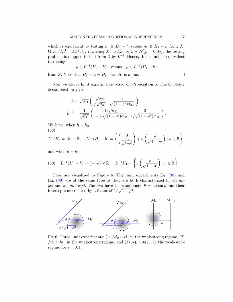
They are visualized in Figure 6. The limit experiments Eq. (38) andEq. (39) are of the same type as they are both characterized by an an-gle and an intercept. The two have the same angle θ = arcsin ρ and theirintercepts are related by a factor of 1/

√1− ρ2.

M0

M1

θ = arcsin ρ

γ/√

1− ρ2

M1

M0

θ = arcsin ρ

γ

Mi M1−i

δ

Fig 6: Three limit experiments: (1)M0 \M1 in the weak-strong regime, (2)M1 \M0 in the weak-strong regime, and (3) Mi \M1−i in the weak-weakregime for i = 0, 1.


BO

Z

A

C

γ

Z1

M0 M1

Z2d2

d1

θ/2

Fig 7: Derivation of the asymptotic distribution Eq. (24) from the limitexperiment ofM1 \M0 under the weak-strong regime (the middle panel ofFig. 6).

Now we prove the form of the asymptotic distributions in Proposition 2from the limit experiment.

Proof of Proposition 2. Since the limit experiments are of the same

type, we only derive for local alternatives Σ(1)n ∈M1 \M0. We set the coor-

dinate system as in Fig. 7, where the bisector of angle ∠BCA = θ = arcsin ρis the y-axis. The standard Gaussian vector centered at B is represented as

Z = (x, y) = (γ sin(θ/2)−Z1, Z2). By the limit experiment, we have λ(0:1)n

d⇒d2

1 − d22. M0 and M1 are respectively represented by lines y = ±kx+ a for

k = cot(θ/2) and a = −γ cos(θ/2). We have

d21 − d2

2 =(a+ kx− y)2

1 + k2− (a− kx− y)2

1 + k2

= 2ρ(Z1 − γ sin(θ/2))(Z2 + γ cos(θ/2)),

where we used2k

1 + k2=

2 cot(θ/2)

1 + cot2(θ/2)= sin θ = ρ.


By a change of variables (Z1, Z2) =d ((U +V )/√

2, (U −V )/√

2) for anotherpair of independent standard normals and using the fact√

1 +√

1− ρ2 −√

1−√

1− ρ2 =√

2(1− ρ),

upon simplifying we have

λ(0:1)n

d⇒ d21 − d2

2 =d ρ

(U + γ

√1− ρ

2

)2

−

(V + γ

√1 + ρ

2

)2 .

4.3.2. The weak-weak regime. The Gaussian limit in Proposition 3 showsthat the limit experiment of the weak-weak regime is testing the location ofa univariate normal between two points; see the last panel of Fig. 6.

Corollary 2. Testing M0 versus M1 under√nρ12,nρ13,n → δ for

δ 6= 0 with ρ12,n, ρ13,n → 0 is asymptotically equivalent to testing H0 : µ = 0versus H1 : µ = δ from a single observation Z ∼ N (µ, 1).

5. Envelope distributions. Though it may at first appear otherwise,the asymptotic distributions as obtained in Proposition 2 and Proposition 3are not directly applicable to forming decision rules. This is due to the non-uniformity of the asymptotics.

Firstly, the asymptotic depends on the regime: weak-strong versus weak-weak, namely where the local sequence converges to. And the law is dis-continuous between the two regimes. That is, the law in the weak-strongregime (scaled difference of noncentral chi-squares) does not converge tothat of the weak-weak regime (Gaussian) as ρ → 0. Furthermore, a pro-cedure that firstly estimates the regime and then uses the correspondingdistribution to form decision boundary, is susceptible to irregularity issues.Additionally, it is difficult to judge if an edge is weak based on whether itsconfidence interval contains zero without further assumptions, as illustratedby the following example.

Example 1. Suppose Xiiid∼ N (γ/

√n, σ2) for i = 1, · · · , n. The usual

(1−α)-level confidence interval for the mean of X is Xn± zα/2σn/√n. The

probability that it contains zero is

Pr(0 ∈ (Xn ± zα/2σn/

√n))

= Pr(√nXn/σn ∈ (±zα/2)

)→ Pr(Z + γ ∈ (±zα/2)) < 1− α


for γ 6= 0 and Z ∼ N (0, 1). A large enough γ can be chosen to make thisprobability arbitrarily small.

Secondly, given the regime, the distribution depends on the value of alocal parameter (γ for strong-weak and δ for weak-weak), which determineshow the local sequence converges. Due to the

√n factor, the standard error

for its estimator does not vanish and in general the local parameter can-not be consistently estimated. The reader is referred to Berger and Boos(1994); Andrews (2001) for discussions in the literature on the treatment ofasymptotic distributions involving nuisance parameters that are not point-identified. Here we take a different approach, presented as follows.

The non-uniformity of asymptotic distributions motivates us to seek aprocedure that circumvents the inference on the regime and the local pa-rameter. In this section, we study the “extremal” distributions arising fromthe asymptotic distributions as the local parameter varies in R.

Definition 1. Given a family of distribution functions Fh : h ∈ Hon R, define

F ∗(x) = suph∈H

Fh(x),

and

(40) F (x) =

F ∗(x), F ∗ is continuous at x

limy→x+ F∗(y), F ∗ is discontinuous at x

.

We call F the envelope distribution of Fh : h ∈ H if F is a valid distribu-tion function.

Lemma 3. F ∗(x) is left-continuous if every Fh(x) for h ∈ H is contin-uous.

Proof. Fix any x and δ > 0, for ε > 0 we have |F ∗(x) − F ∗(x − ε)| =suph Fh(x)− suph Fh(x− ε). By definition of supremum, there exists h′ ∈ Hsuch that Fh′(x) ≥ suph Fh(x) − δ/2. Hence, |F ∗(x) − F ∗(x − ε)| ≤ δ/2 +Fh′(x)− Fh′(x− ε). By continuity of Fh′ , choosing ε > 0 such that Fh′(x)−Fh′(x− ε) ≤ δ/2 shows that F ∗(x) is left-continuous.

Lemma 4. If F ∗(x) → 0 as x → −∞, then F (x) is a valid distributionfunction.

Proof. Given any x ≤ x′, suph Fh(x) ≤ suph Fh(x′) by monotonicity ofevery Fh. Since F ∗ is non-decreasing, by Folland (1999, Theorem 3.23), the


set of points at which F ∗ is discontinuous is countable. By redefining thefunction value at these points to be their right limits, F is right continuous.Also, F (x) ≥ F ∗(x) → 1 as x → +∞ since every Fh(x) → 1. Finally, asx→ −∞ if F ∗(x)→ 0 , then F (x)→ 0. F is a distribution function.

5.1. The weak-weak regime.

Proposition 7. Let Gδ = N (δ2, (2δ)2) : δ ∈ R be the asymptoticdistributions for the weak-weak regime under M0 \ M1. The envelope ofGδ is an equal-probability mixture of (−χ2

1) and a point mass at zero,namely

(41) G(x) =1

2

(1− Fχ2

1(−x)

)Ix<0 +

1

2Ix≥0

The corresponding envelope under M1 \M0 is distributed as its negation.

Proof. It suffices to consider δ ≥ 0. Given any x < 0,

supδ

Pr(δ2+2δZ ≤ x) = supδ>0

Φ

(x− δ2

2δ

)= sup

δ>0Φ

(−[−x2δ

+δ

2

])= Φ(−

√−x),

where δ∗ =√−x is the maximizer; Given any x ≥ 0, δ = 0 maximizes the

probability to one. Hence, the envelope CDF is

G(x) =

Φ(−√−x), x < 0

1, x ≥ 0,

from which it follows that

g(x) = G′(x) =1

2fχ2

1(−x)Ix<0 +

1

2δ0(x).

The envelope for M1 \M0 follows from symmetry.

Since whenM0 is true, the region for rejectingM0 should take the form(−∞, r) for some r < 0, only the negative part of G is relevant for decisionmaking. It follows from Proposition 7 that the negative part of G is dis-tributed as χ2

1. The formation of the envelope is visualized in Fig. 8, whichaligns with the behavior observed in Fig. 4, where as δ grows, the quantilesfor α = 0.05 first moves outward for δ ∈ (0.5, 1.64) and then moves inwardfor δ ∈ (1.64,∞).


0.00

0.25

0.50

0.75

1.00

−5.0 −2.5 0.0 2.5x

cum

ulat

ive

prob

abili

ty

δ00.10.250.50.7511.524Envelope

Envelope of N(δ2,(2δ)2)

Fig 8: The envelope CDF G for the weak-weak regime.

5.2. The weak-strong regime. Now we study the envelope distributionsunder the weak-strong regime. We first observe that the envelope distribu-tions, if they exist, must be symmetric for Eq. (23) and Eq. (24), in the sensethat they are distributed as the negation of each other. The symmetry holdsbecause the two local parameters are related by a factor of 1/

√1− ρ2 (see

Fig. 6), and hence the suprema are taken over the same set of laws up to adifference in the sign. Fix ρ, let Fρ,γ : γ ∈ R be the family of asymptoticdistributions in the weak-strong regime underM0\M1 as given in Eq. (23).Let Fρ be its envelope distribution function.

Proposition 8. Fρ is a valid distribution function for |ρ| ∈ (0, 1].

Proof. Note since Fρ = F−ρ, it suffices to consider ρ ∈ (0, 1]. First con-

sider ϕρ,γ(x), the density function forX2−Y 2 withX ∼ N(µ1 = γ

√1−ρ

2 , 1

)and Y ∼ N

(µ2 = γ

√1+ρ

2 , 1

)for γ ∈ R and ρ ∈ (0, 1]. Since p(X2 − Y 2 =

v2, Y 2 = t) = p(Y 2 = t)p(X2 = t + v2), the density ϕρ,γ has the followingintegral representation from marginalization

ϕρ,γ(v2) =

∫ ∞0

χ21(t;µ2

2)χ21(v2 + t;µ2

1) dt

=1

2πe−v

2/2−γ2/2∫ ∞

0

exp(−t) cosh(γ√

1+ρ2

√t) cosh(γ

√1−ρ

2

√t+ v2)√

t(t+ v2)dt.


Recall that . allows for a positive multiplicative constant. Using cosh(x) <exp(x) for x > 0, we have

ϕρ,γ(v2) . e−v2/2−γ2/2

∫ ∞0

e−t cosh(γ√

1+ρ2

√t) cosh(γ

√1−ρ

2

√t+ v2)√

t(t+ v2)dt

< e−v2/2

∫ ∞0

exp

(−t− γ2/2 + γ

√1+ρ

2

√t+ γ

√1−ρ

2

√t+ v2

)√t(t+ v2)

dt.

We note that

−γ2/2+γ

√1 + ρ

2

√t+γ

√1− ρ

2

√t+ v2 ≤ 1

2

(√1 + ρ

2

√t+

√1− ρ

2

√t+ v2

)2

by completing the square in γ. It then follows that

ϕρ,γ(v2) < e−v2/2

∫ ∞0

exp[−t+ 1

2

(t+ 1−ρ

2 v2 +√

1− ρ2√t(t+ v2)

)]√t(t+ v2)

dt

= e−1+ρ4v2∫ ∞

0

exp

(− t

2 +

√1−ρ22

√t(t+ v2)

)√t(t+ v2)

dt

≤ e−1+ρ4v2∫ ∞

0

exp

(− t

2 +

√1−ρ22 (t+ v2/2)

)√t(t+ v2)

dt

= e−1+ρ−

√1−ρ2

4v2∫ ∞

0

exp

(−1−√

1−ρ22 t

)√t(t+ v2)

dt

= e−ρ4v2K0

(1−

√1− ρ2

4v2

),

where we used 2√t(t+ v2) ≤ 2t + v2 in the third line. Kν(·) is the mod-

ified Bessel function of the second kind, and has the following asymptoticexpansion for z > 0 (Abramowitz and Stegun, 1972, Page 378)

Kν(z) =

√π

2ze−z(1 +

4ν2 − 1

8z+O(z−2)).

Hence for large v2, we have

ϕρ,γ(v2) .exp

(−1+ρ−

√1−ρ2

4 v2

)(1−

√1− ρ2)v2

.


Recall that Fρ,γ : γ ∈ R is the family of distributions for the RHS of

Eq. (23). With γ′ =√

1− ρ2γ,

ρ

(Z1 + γ

√1 + ρ

2

)2

−

(Z2 + γ

√1− ρ

2

)2 ∼ Fρ,γ′ .

It follows that the density function

(42) fρ,γ′(−v2) = ϕρ,γ(v2/ρ) .ρ exp

(−1+ρ−

√1−ρ2

4ρ v2

)(1−

√1− ρ2)v2

,

where the exponent1+ρ−√

1−ρ24ρ ∈ (1/4, 1/2]. By Definition 1, we have

F ∗ρ (−v2) = supγ′∈R

Fρ,γ′(−v2)

= supγ′∈R

∫ ∞v2

fρ,γ′(−u) du .∫ ∞v2

ρ exp

(−1+ρ−

√1−ρ2

4ρ u

)(1−

√1− ρ2)u

du <∞,

and hence F ∗ρ (−v2) → 0 as v → ∞. By Lemma 4, Fρ is a distributionfunction for every ρ ∈ (0, 1].

The following proposition shows that Fρ,γ=0 constitutes the envelope forthe positive part of Fρ.

Proposition 9. The positive part of Fρ for |ρ| ∈ (0, 1] is distributed as

the positive part of ρ(Z21 − Z2

2 ) for Z1, Z2iid∼ N (0, 1).

Proof. Fix ρ ∈ (0, 1] and v2 ≥ 0, with γ′ = γ√

1− ρ2 it follows fromProposition 2 that

(43) 1− Fρ,γ′(v2) = Pr((Z1 + µ1)2 − (Z2 + µ2)2 ≥ v2/ρ

),

where µ1 = γ√

(1 + ρ)/2, µ2 = γ√

(1− ρ)/2. Since Fρ,γ′ is symmetricin γ, we show γ = 0 maximizes Fρ,γ′(v

2) by showing that the probabil-ity on the RHS of Eq. (43) increases in γ ∈ (0,∞). The probability canbe interpreted as the standard Gaussian measure of the hyperbolic set(x, y) : x2 − y2 ≥ v2/ρ with the Gaussian centered at G = (µ1, µ2) =γ(√

(1 + ρ)/2,√

(1− ρ)/2). This is visualized in Fig. 9, where γ = OG,tanφ =

√(1− ρ)/(1 + ρ) and the hyperbolic set consists of the area inside


the two branches. As γ increases from zero, the center moves away from theorigin along the V line. Let U be the line perpendicular to V . The Gaussianmeasure has two independent standard normal projections (U, V ), which isa rotation of (Z1, Z2). Now we show that for every v > 0, by conditioningon |V | = v, the conditional probability of U in the appropriate “section” ofthe hyperbolic set, denoted by probability q(v), increases with γ.

Let [A,B] and [C,D] be the line segments that V = −v and V = vintersect the hyperbola respectively. By independence of U and V , we haveq(v) = Pr(U ∈ [A,B]) + Pr(U ∈ [C,D]). Let v and v be the distance fromG to the tangent to the left and right branch of the hyperbola respectively,parallel to line U ; see Fig. 9. There are three cases. (i) When v ≤ v (the firstpanel of Fig. 9), as γ increases, both [A,B] and [C,D] become bigger, andthus q(v) increases. (ii) When v < v ≤ v, [A,B] is empty but [C,D] becomesbigger, so q(v) increases. (iii) When v > v, as γ increases (the second panelof Fig. 9), [C,D] increases but [A,B] decreases. Let [E,F ] be the segmentsymmetric to [A,B] about the origin. We observe that, as γ increases byan infinitesimal ∆γ, the amount that Pr(U ∈ [A,B]) decreases equals theamount that Pr(U ∈ [E,F ]) increases, which is smaller than the amountthat Pr(U ∈ [C,D]) increases. Hence, q(v) still increases.

By the monotonicity for every value of |V |, we conclude that the to-tal probability on the RHS of Eq. (43) increases in γ. Hence, Fγ,ρ(v

2) ismaximized at γ = 0 for every v, namely Fρ = Fρ,γ=0. It follows that forX ∼ Fγ , (X)+ =d ρ(Z2

1 − Z22 )+ for two independent standard normal vari-

ables Z1, Z2.

Corollary 3. Fρ(0) ≡ 1/2.

Unfortunately, we do not have an analytic form of the distribution for thenegative part of Fρ, which is the part relevant for decision making, exceptfor ρ→ 0 and ρ = 1.

Proposition 10 (Bessel envelope). Fρ=1 =d Z21 − Z2

2 for Z1, Z2iid∼

N (0, 1).

Proof. Under ρ = 1, the CDF is

Fγ(x) = Pr((Z1 + γ)2 − Z2

2 ≤ x)

= EZ2 Pr((Z1 + γ)2 ≤ x+ Z2

2 | Z2

).

Since the conditional probability is non-negative, it suffices to show thatgiven any x ∈ R, γ = 0 maximizes Pr

((Z1 + γ)2 ≤ x+ z2

2 | Z2 = z2

)=

Pr((Z1 + γ)2 ≤ x+ z2

2

)for all z2 ∈ R. When x + z2

2 ≤ 0, the conditional


x

y

V

Uv

D

C

B

AO

Gφ

x

y

V

U

v

C

D

F

E

B

A

O

Gφ

Fig 9: The CDF Fρ,γ(·) at can be interpreted as the probability of a hyper-bolic set (inside the two branches of blue curves) as measured by a standardnormal centered |γ| away from the origin, lying on the line V with slopetanφ =

√(1− ρ)/(1 + ρ). The asymptotes of the hyperbola are y = ±x.

probability is zero and γ = 0 is trivially a maximizer. When x+z22 > 0, then

Pr((Z1 + γ)2 ≤ x+ z2

2

)= Φ(

√x+ z2

2 − γ)−Φ(−√x+ z2

2 − γ). Setting the

derivative with respect to γ to zero requires φ(−√x+ z2

2−γ) = φ(√x+ z2

2−γ), to which γ = 0 is the unique solution. Therefore, γ = 0 is the unique


maximizer of Fγ(x) for all x.

The distribution in Proposition 10 is a difference between two independentχ2

1 variables. The density, as plotted in Fig. 10, is

pB(u) =1

2πK0(|u|/2),

where K0 is a modified Bessel function of the second kind. It is referred toas a K-form Bessel distribution in the literature; see Johnson et al. (1995,Chapter 4.4), Bhattacharyya (1942) and Simon (2007, Page 25).

0.00

0.25

0.50

0.75

−4 −2 0 2 4x

PD

F o

f Bes

sel K

−fo

rm

Fig 10: The density for Fρ=1 =d Z21 − Z2

2 .

Proposition 11 (Continuity of envelope). Fρd⇒ G as ρ→ 0, where G

is the envelope distribution for the weak-weak regime given in Proposition 7.

Proof. Firstly, we note that Fρ(0) = G(0) = 1/2 and by Proposition 9the non-negative part of Fρ also converges to that of G as ρ → 0, namelya point mass at zero. It remains to be shown that the negative part of Fρconverges in law to the negative part of G. It suffices to show for any x ≤ 0

supγ

Pr

ρ(Z1 + γ

√1 + ρ

2

)2

−

(Z2 + γ

√1− ρ

2

)2 ≤ x

→ Pr(−Z2 ≤ x)/2


as ρ→ 0. Given ρ > 0, the maximized probability can be rewritten as

supγ

Pr

ρ(Z1 + γ

√1 + ρ

2

)2

−

(Z2 + γ

√1− ρ

2

)2 ≤ x

= sup

γPr

((γρ)2 + 2γρ

(√1 + ρ

2Z1 −

√1− ρ

2Z2

)≤ x− ρ(Z2

1 − Z22 )

)

= supδ

Pr

(δ2 + 2δ

(√1 + ρ

2Z1 −

√1− ρ

2Z2

)+ ρ(Z2

1 − Z22 ) ≤ x

)= sup

δPr (Xρ(δ) ≤ x) ,

where we define

Xρ(δ) := δ2 + 2δ

(√1 + ρ

2Z1 −

√1− ρ

2Z2

)+ ρ(Z2

1 − Z22 )

for ρ ∈ [0, 1) and δ ∈ R. Note that supδ Pr(X0(δ) ≤ x) = supδ Pr(δ2 +2δZ ≤x) = Pr(−Z2 ≤ x)/2 for Z ∼ N (0, 1) by Proposition 7. We are left to showsupδ Pr (Xρ(δ) ≤ x) → supδ Pr (X0(δ) ≤ x) as ρ → 0. Choose x < M < ∞and define

Yρ(δ) :=

Xρ(δ), Xρ(δ) ≤MM, Xρ(δ) > M

.

We observe that ∣∣∣∣supδ

Pr (Xρ(δ) ≤ x)− supδ

Pr (X0(δ) ≤ x)

∣∣∣∣=

∣∣∣∣supδ

Pr (Yρ(δ) ≤ x)− supδ

Pr (Y0(δ) ≤ x)

∣∣∣∣≤ sup

δ|Pr (Yρ(δ) ≤ x)− Pr (Y0(δ) ≤ x)|

= supδ

∣∣E (IYρ(δ)≤x − IY0(δ)≤x)∣∣→ 0,

where the last step follows from weak convergence Yρ(δ) : δ ∈ R Y0(δ) :δ ∈ R in `∞(R) as ρ → 0 for a bounded stochastic process; see van derVaart (2000, Chap. 18).

Perhaps surprisingly, Proposition 11 shows that the asymptotic envelopeis continuous between the two regimes, which bridges the discontinuity of

the asymptotic distributions of λ(0:1)n as presented in Propositions 2 and 3.


Therefore, taking the envelope resolves the non-uniformity issue in termsof both the regime and the local parameter. Now with this we extend thedefinition of the envelope Fρ to ρ ∈ [0, 1] by writing Fρ=0 = G.

ρ = 0.3 ρ = 0.7

−5 0 −5 0

0.00

0.25

0.50

0.75

1.00

x

cum

ulat

ive

prob

abili

ty

γ0.10.511.522.53468envelope

Envelope of Fρ,γ

Fig 11: The envelope distribution Fρ under the strong-weak regime for ρ =0.3, 0.7.

Figure 11 showcases two envelopes. In the absence of an analytic formfor ρ ∈ (0, 1), the envelopes can be numerically simulated by taking thesupremum over a grid of values for γ. We observe from simulations thatthere exists γ∗(x, ρ) ∈ (0,∞) such that ±γ∗ uniquely maximizes Fγ,ρ(x).

Finally, we conclude this section by noting the following envelope of en-velopes. See Figure 12 for an illustration. This result will be used in the nextsection to form simple decision rules based on the Bessel distribution.

Proposition 12 (Envelope of envelopes). The negative part of the en-velope of Fρ : ρ ∈ [0, 1] is distributed as the negative part of Fρ=1 (Bessel).

6. Model selection procedures. Since we are selecting between twonon-nested models, we want to refrain from choosing one of them as thedefault (the null hypothesis). By treating M0 and M1 symmetrically, how-ever, a procedure that takes output value in M0,M1 cannot simultane-ously control both types of error under a given tolerance. It can be seenfrom Figs. 2 and 5 that there are cases where the asymptotic distributions

of λ(0:1)n under P

Σ(0)n

and PΣ

(1)n

significantly overlap. In such cases, insisting

on a dichotomous choice will inevitably result in a high probability of errorunder at least one model.


0.00

0.25

0.50

0.75

1.00

−5.0 −2.5 0.0 2.5x

enve

lope

CD

F

ρ0.10.30.50.70.91

Fig 12: The negative part of envelope of Fρ : ρ ∈ [0, 1] is the negative partof Fρ=1.

To deal with this possible indistinguishability, we opt for a procedure withthree options: if two models can be sufficiently distinguished, it selects one ofthem; otherwise it refrains from commitment by selecting both models, for-mally denoted as the union M0 ∪M1. It is worth stressing that we alwaysassume at least one of the two models is true. By such a design, when theprocedure does not output the union, we are ensured that the probability ofchoosing the wrong model is small, being controlled below a given toleranceα. In contrast, in the usual hypothesis testing framework where supposedlyM0 is the null and M1 is the alternative, one typically cannot simultane-ously control both type-I and type-II error. In other words, our procedureselects model with “confidence”. Recently the same notion has been inves-tigated by Lei (2014) in a classification setting; Robins et al. (2003) alsoallows a test to make no decision when faced with ambiguity. We formalizethe concept as follows.

Suppose (X1, X2, X3) ∈ Rn×3 consists of n independent samples fromN (0,Σn), where Σn ∈M0 ∪M1 is allowed to change with n and Σn → Σ∗.The sequence Σn models signal strength relative to the sample size. Weconsider a deterministic decision rule

(44) φn(Sn) : R3×3PSD → M0,M1,M0 ∪M1,

where sample covariance Sn is the sufficient statistic. For a given sequenceof Σn ∈Mi \M1−i with Σn → Σ∗ ∈Mi ∪M1−i, we define the asymptotic


(type-I) error of φn as the large-sample probability of rejecting the truemodel, i.e.,

(45) perr((Σn)) := lim supn→∞

Pr(φn(Sn) =M1−i),

where the probability is taken under PnΣn . Similarly, the asymptotic poweris defined as

(46) ppow((Σn)) := lim infn→∞

Pr(φn(Sn) =Mi).

We say that the error is uniformly controlled below a given size α > 0, if

(47) p(0)err := sup

(Σ(0)n )

perr((Σ(0)n )) ≤ α and p(1)

err := sup(Σ

(1)n )

perr((Σ(1)n )) ≤ α,

where for i = 0, 1 the supremum for (Σ(i)n ) is taken over all converging

sequences of Σ(i)n within Mi \M1−i (the limit can be in either Mi \M1−i

or Mi ∩M1−i). In general, the power ppow((Σn)) depends on the sequenceconsidered and we do not seek power optimality or guarantee in a uniformsense. In the next section, we will compare the power of several proposedprocedures to the theoretical optimal for Σn considered in the two regimesof local asymptotics.

By construction, using the α-quantile of the envelope as the decisionboundary achieves uniform error control. Based on the envelope of envelopes,a simple uniform rule is

(48) φunifn =

M0, λ

(0:1)n > −F−1

ρ=1(α)

M1, λ(0:1)n < F−1

ρ=1(α)

M0 ∪M1, otherwise

.

To gain more power, since Fρ is continuous in ρ and ρ can be consistentlyestimated (recall that ρ = ρstrong in the weak-strong regime, and ρ = 0 inthe weak-weak regime), an adaptive rule can be formed as

(49) φadan =

M0, λ

(0:1)n > −F−1

ρn(α)

M1, λ(0:1)n < F−1

ρn(α)

M0 ∪M1, otherwise

,

where ρn = |ρ13,n| ∨ |ρ23,n| is the MLE for |ρ|. If it is desired to report a p-

value, consider a potentially conservative p-value = Fρ(−|λ(0:1)n |). For ρ = 1


and ρ = ρn respectively, the uniform rule and the adaptive rule can be thenrestated as

φn =

M0, λ

(0:1)n > 0 and p-value < α

M1, λ(0:1)n < 0 and p-value < α

M0 ∪M1, otherwise

.

The conservative p-value can be computed numerically by Monte Carlo andthen taking the maximum over a grid of values for γ.

Theorem 1. The adaptive rule φadan controls asymptotic error uniformlybelow α for 0 < α < 1/2.

Proof. We show error guarantee when M0 is true. The same argumentholds when M1 is true. It suffices to show for any converging sequenceΣn ∈M0 \M1,

perr((Σn)) = lim supn→∞

Pr(φn(Sn) =M1) ≤ α,

where the probability is measured under PnΣn . Suppose Σn → Σ∗ ∈M0∪M1.

If Σ∗ /∈ M0 ∩ M1, then λ(0:1)n is unbounded in probability towards +∞.

Hence Pr(φn(Sn) = M0) → 1 and perr(Σn) = 0. In the following we provethe claim for Σ∗ ∈M0∩M1. Suppose ρij,n, ρij,n and ρij respectively denotethe corresponding correlation coefficient of Sn, Σn and Σ∗. We have threecases depending on the rate at which Σn converges.

1. When |ρ13,nρ23,n| 1/√n, there are two regimes depending on Σ∗.

(a) In the weak-strong regime, without loss of generality suppose√nρ13,n → γ 6= 0 and ρ23,n → ρ 6= 0. By consistency ρn =|ρ13,n| ∨ |ρ23,n| →p |ρ| and the definition of envelope, we have

lim supn

Pr(λ(0:1)n < F−1

ρn(α)) = Fγ,ρ(F

−1ρ (α)) ≤ Fγ,ρ(F−1

γ,ρ (α)) = α.

(b) In the weak-weak regime, suppose√nρ13,nρ23,n → δ 6= 0. We

have ρn = |ρ13,n| ∨ |ρ23,n| = (|ρ13,n| ∨ |ρ23,n|) + Op(1/√n) →p 0

since both ρ13,n, ρ23,n → 0. By Proposition 11, we have

lim supn

Pr(λ(0:1)n < F−1

ρn(α)) = Gδ(F

−1ρ=0(α))

= Gδ(G−1(α)) ≤ Gδ(G−1

δ (α)) = α.


2. When |ρ13,nρ23,n| = o(1/√n), we have λ

(0:1)n →p 0. Since F−1

ρ (α) <c < 0 for α < 1/2, we have Pr(φn(Sn) =M0 ∪M1)→ 1.

3. When |ρ13,nρ23,n| = ω(1/√n), we have Pr(λ

(0:1)n > c) → 1 for any

constant c and hence Pr(φn(Sn) =M0)→ 1.

As can be seen from the proof, the consistency of model selection based onthe loglikelihood (or AIC/BIC since in this caseM0 andM1 have the samedimensions) is a special case when |ρ13,nρ23,n| = ω(n−1/2), i.e., under strongsignal or large enough sample size. However, under |ρ13,nρ23,n| = O(n−1/2),simply choosing the model with the highest loglikelihood (or the lowestAIC/BIC) can lead to large errors, as we will illustrate in the next section.Note that Theorem 1 provides a “rate-free” guarantee, in the sense thatit does not require any a priori assumption on the rate of signal strengthrelative to the sample size. The envelope of envelopes leads to the sameguarantee for the uniform rule.

Corollary 4. The decision rule φunifn controls asymptotic error uni-formly below α for 0 < α < 1/2.

Proof. It follows from Theorem 1 and Proposition 12.

The uniform rule can be easily applied by comparing the difference in log-likelihoods to a single number, e.g., 3.19 for α = 0.05 and 5.97 for α = 0.01.The adaptive rule can be implemented by numerically evaluating F−1

ρ (α)via Monte Carlo on a grid of ρ and interpolating. Some values are plottedin Fig. 13 and tabulated in Table 1 based on 107 samples. It is interestingto notice that F−1

ρ (α) is not monotonic in ρ ∈ [0, 1].

Table 1Envelope quantiles −F−1

ρ (α), Monte Carlo standard errors ≤ 0.01

ρ 0.0 0.1 0.2 0.3 0.4 0.5 0.6 0.7 0.8 0.9 1.0

α = 0.05 2.71 2.71 2.68 2.65 2.58 2.48 2.42 2.39 2.58 2.90 3.19α = 0.01 5.41 5.41 5.40 5.34 5.27 5.21 5.11 5.05 5.02 5.40 5.97

7. Simulations. In this section we conduct numerical simulations toassess the performance of the adaptive and uniform decision rules proposedin the previous section. In subsequent simulations we use α = 0.05. In addi-tion to the two methods we propose, we also consider the following methodsfor comparison.


3

4

5

6

0.00 0.25 0.50 0.75 1.00ρ

enve

lope

qua

ntile

s α0.010.05

linetypeBesselchi square

Fig 13: Negated α-quantiles of Fρ evaluated on a grid.

Naive. The naive procedure selects the model with a higher likelihood (orequivalently, a lower AIC/BIC, since M0 and M1 have the same dimen-sions), namely

φnaiven =

M0, λ

(0:1)n > 0

M1, λ(0:1)n < 0

.

This is effectively choosing a single model based on AIC/BIC since thepenalty terms cancel out as M0 and M1 have the same dimension.

Interval Selection. This method is adapted from Drton and Perlman (2004).We construct (1−α)-level non-simultaneous confidence intervals on correla-tion coefficients ρ12 and ρ12·3 with Fisher’s z-transform (Fisher, 1924). Thedecision rule is

(50) φintervaln =

M0, 0 ∈ C.I.(ρ12) and 0 /∈ C.I.(ρ12·3)

M1, 0 ∈ C.I.(ρ12·3) and 0 /∈ C.I.(ρ12)

M0 ∪M1, otherwise

.

Note that the interval selection method controls asymptotic error below α.For example, when M0 is true,

lim supn

Pr(φintervaln =M1) ≤ lim sup

nPr(0 /∈ C.I.(ρ12)) ≤ α.

We conduct numerical simulations in the following three settings.

7.1. Local hypotheses. We simulate under Σ(0)n and Σ

(1)n (variances are set

to unity) for the two regimes considered in Section 4. The power is compared


to the theoretically optimal. Since exact values of the total variation distanceare intractable, we plot bounds given by Eq. (16) in grey curves. We perform4,000 replications for each point on the graphs.

See Figures 14 and 15 for the size and power in the weak-strong regime(Eqs. (21) and (22)) under n = 1, 000. Smaller sample sizes n = 100, 200, . . .generate very similar results. See Figure 16 for the size and power in theweak-weak regime (Eqs. (25) and (26)), where we set ρ13,n = n−a/4, ρ23,n =n−1/2+a/4 and let a vary. We observe that (i) the naive method does notcontrol error at all; (ii) the other three methods control error uniformlyeven under relatively small n. We also observe that the relation “adaptive”> “uniform” > “interval” holds in general in terms of both size and power.By comparing to the grey curves, we regard the adaptive rule as achievingnear-optimal power in these settings.

7.2. Projected Wishart. We generate a covariance matrix by firstly draw-ing Σ from the Wishart distribution (with the scale matrix chosen as σij =(−1/2)|i−j|) and then projecting Σ into M0 or M1 respectively by findingthe MLE under each model. Then we perform model selection based ontwo sets of zero-mean Gaussian samples generated with the two projectedcovariances respectively. We vary the degrees of freedom for the Wishartdistribution. See Figure 17 for the results.

7.3. Conditional on covariates. We consider the common regression set-ting where two types of independences are contrasted conditional on a setof covariates X ∈ Rp. In other words, we want to select betweenM0 : Y1 ⊥⊥Y2 | X and M1 : Y1 ⊥⊥ Y2 | Y3, X. We generate instances by

(51) (Y1, Y2, Y3) = Xᵀ(β1, β2, β3) + E, E ∼ N (0,Σ),

where we use the previous projected Wishart to generate error covarianceΣ under M0 and M1. We perform model selection by firstly regressing(Y1, Y2, Y3) onto X with least squares and then apply the model selec-tion procedures to the residual covariance. Covariates are randomly drawnfrom standard Gaussians and regression coefficients are generated from at-distribution with 4 degrees of freedom. We fix n = 1, 000 and vary thenumber of covariates p. The results are presented in Figure 18. We observethat the proposed procedure continues to maintain nominal size until p isrelatively large compared to n. The power performance, on the other hand,does not seem to vary much as p grows.

8. Real data example. In this section we showcase an example ofapplying the method to edge orientation in learning a DAG. In studying the


γ = 0.1 γ = 1 γ = 2 γ = 3 γ = 4M

0\M1

M1\M

0

0.0 0.5 1.0 0.0 0.5 1.0 0.0 0.5 1.0 0.0 0.5 1.0 0.0 0.5 1.0

0.00

0.02

0.04

0.06

0.00

0.02

0.04

0.06

|ρstrong|

size

methodadaptiveintervaluniform

n = 1000, 4000 replicates, α = 0. 05

size of procedure under different values of γ

γ = 0.1 γ = 1 γ = 2 γ = 3 γ = 4

M0

\M1

M1

\M0

0.0 0.5 1.0 0.0 0.5 1.0 0.0 0.5 1.0 0.0 0.5 1.0 0.0 0.5 1.0

0.0

0.2

0.4

0.0

0.2

0.4

|ρstrong|

siz

e

method

adaptive

interval

uniform

naive

n = 1000, 4000 replicates, α = 0. 05

size of procedure under different values of γ

Fig 14: Size Pr(φn = M1−i|Mi) of the procedures (with 95% confidenceintervals) under the weak-strong regime of local hypotheses. α = 0.05 ismarked as dashed. The naive method is only included in the second plot forbetter visualization.


γ = 0.1 γ = 1 γ = 2 γ = 3 γ = 4

M0\M

1M

1\M0

0.0 0.5 1.0 0.0 0.5 1.0 0.0 0.5 1.0 0.0 0.5 1.0 0.0 0.5 1.0

0.00

0.25

0.50

0.75

1.00

0.00

0.25

0.50

0.75

1.00

|ρstrong|

pow

er

linetypelower boundupper bound


power of procedure under different values of γ

Fig 15: Power Pr(φn = Mi|Mi) of the procedures (with 95% confidenceintervals) under the weak-strong regime of local hypotheses. α = 0.05 ismarked as dashed. Grey curves are bounds on the theoretically optimalpower.

American occupational structure, Blau and Duncan (1967) measured thefollowing covariates on n = 20, 700 subjects:

V : father’s educational attainment,X: father’s occupational status,U : child’s educational attainment,W : status of child’s first job,Y : status of child’s occupation in 1962.

The data is summarized as the following correlation matrix of (V,X,U,W, Y )

Sn =

1.000 0.516 0.453 0.332 0.3220.516 1.000 0.438 0.417 0.4050.453 0.438 1.000 0.538 0.5960.332 0.417 0.538 1.000 0.5410.322 0.405 0.596 0.541 1.000

.

At level α = 0.01, the PC algorithm identifies the skeleton by d-separation,which only removes the edge between V and Y based on Y ⊥⊥ V | U,X. Thisis because the PC algorithm tests for conditional independence given smallerconditioning sets first. By a common-sense temporal ordering V,X < U <W,Y among the variables, edges can be oriented except for X − V and


n = 20 n = 50 n = 100 n = 500 n = 1000M

0\M1

M1\M

0

0 0.5 1 0 0.5 1 0 0.5 1 0 0.5 1 0 0.5 1

0.010.020.030.040.050.06

0.010.020.030.040.050.06

a

size


4000 replicates, α = 0. 05

size of procedure under ρ13=n−a/4, ρ23=n−1/2+a/4

n = 20 n = 50 n = 100 n = 500 n = 1000

M0\M

1M

1\M0

0 0.5 1 0 0.5 1 0 0.5 1 0 0.5 1 0 0.5 1

0.00

0.25

0.50

0.75

0.00

0.25

0.50

0.75

a

pow

er

linetypelower boundupper bound


power of procedure under under ρ13=n−a/4, ρ23=n−1/2+a/4

Fig 16: Size Pr(φn =M1−i|Mi) and power Pr(φn =Mi|Mi) of the proce-dures (with 95% confidence intervals) under the weak-weak regime of localhypotheses (ρ13,nρ23,n = n−1/2). α = 0.05 is marked as dashed. Grey linesare bounds on the theoretically optimal power in the second plot. The naivemethod is excluded due to its large type-I error.


n = 20 n = 50 n = 100 n = 300M

0\M1

M1\M

0

10 20 30 10 20 30 10 20 30 10 20 30

0.000.010.020.030.040.05

0.000.010.020.030.040.05

degrees of freedom

size



size of procedure on the projected Wishart

n = 20 n = 50 n = 100 n = 300

M0\M

1M

1\M0

0 10 20 30 0 10 20 30 0 10 20 30 0 10 20 30

0.25

0.50

0.75

0.25

0.50

0.75

degrees of freedom

pow

er



power of procedure on the projected Wishart

Fig 17: Size Pr(φ =M1−i|Mi) and power Pr(φ =Mi|Mi) of the procedureson projected Wishart matrices (with 95% confidence intervals). α = 0.05 ismarked as dashed. The naive method makes large errors and is excluded.


M0\M1 M1\M0

power

size

0 100 200 300 400 500 0 100 200 300 400 500

0.6

0.7

0.8

0.9

0.00

0.05

0.10

0.15

p

valu

e

methodadaptiveintervaluniformnaive

n = 1000, 1000 replicates, α = 0. 05

size and power conditional on p covariates

Fig 18: Size Pr(φ = M1−i|Mi) and power Pr(φ = Mi|Mi) of the modelselection procedures conditioned on p covariates (with 95% confidence in-tervals). Error covariances are generated from the projected Wishart. Theprocedures are applied to the least-squares residual covariance. α = 0.05 ismarked as dashed.

W − Y ; see Fig. 19. The edge V − X does not involve a collider and theorientation is statistically unidentifiable.

V U

X W

Y

Fig 19: CPDAG inferred from Blau and Duncan (1967) dataset. The skeletonis inferred based on d-separation at level α = 0.01 with the PC algorithm.Blue edges are oriented based on temporal ordering V,X < U < W,Y .

However, the orientation of W−Y raises the interesting question of testing

M0 (Y →W ) : V ⊥⊥ Y | U,X versus M1 (Y ←W ) : V ⊥⊥ Y |W,U,X.

We apply our method to the conditional correlation of (V,W, Y ) given

(U,X). We have λ(0:1)n = 3.72 and p-value = 0.026 under the envelope distri-


bution Fρn . Therefore, under α = 0.01 the adaptive procedure would chooseM0 ∪ M1 and leave the orientation undetermined (the procedure wouldchoose Y → W under α = 0.05). This example illustrates the potentialambiguity in model selection even under a large sample size. The reader isreferred to Spirtes et al. (2000, Section 5.8.4) for another discussion of thesame example.

9. Discussion. We have considered choosing between marginal inde-pendence and conditional independence in a Gaussian graphical model, as-suming we know at least one of them is true. The loglikelihood ratio statisticconverges to a tight law under a sequence of truths converging to the in-tersection of the two models at a certain rate. The asymptotic distributionis shown to be non-uniform as it depends on where and how the sequenceconverges. We address this non-uniformity issue by introducing a family ofenvelope distributions that are well-behaved and bring back the continu-ity of asymptotic laws, as indexed by a parameter that can be consistentlyestimated. Contrary to the usual Neyman–Pearson hypothesis testing, wetreat the two models symmetrically and develop model selection rules thatchoose both models when they are indistinguishable under a given samplesize. Such rules can be designed according to the quantiles of the envelopedistributions to uniformly control the type-I error below a desired level. Asnoted before we believe that “rate-free” asymptotic guarantees that are uni-form are more useful in practice, since they do not rely upon untestableassumptions regarding the sample size and the signal strength.

In this report we restricted ourselves to the Gaussian case. For testingconditional independence, some form of distributional assumption seems in-evitable, since recent work of Shah and Peters (2020) shows that testingconditional independence without restricting the form of conditional inde-pendence is impossible in general.

Selection of non-nested models routinely relies on penalized scores basedon loglikelihoods, such as the negated AIC and BIC. However, as we show,in the context of a weak signal relative to the sample size, simply choosingthe model with the highest score can lead to considerable errors. To selectmodels with “confidence”, one should also look at the “gaps” between thetop scores. We believe that the method developed in this paper may begeneralizable to a wider range of model selection problems.

Acknowledgements. RG thanks Michael Perlman for helpful discus-sions. TR thanks Robin Evans and Peter Spirtes. The research was sup-ported by the U.S. Office of Naval Research.


References.

Milton Abramowitz and Irene A Stegun. Handbook of Mathematical Functions: with For-mulas, Graphs, and Mathematical Tables. Number 55. Courier Dover Publications,1972.

Theodore W. Anderson. An Introduction to Multivariate Statistical Analysis. Wiley NewYork, 2 edition, 1984.

Donald W. K. Andrews. Testing when a parameter is on the boundary of the maintainedhypothesis. Econometrica, 69(3):683–734, 2001.

Ole Barndorff-Nielsen. Information and Exponential Families: in Statistical Theory. JohnWiley & Sons, 2014.

Roger L Berger and Dennis D Boos. P values maximized over a confidence set for thenuisance parameter. Journal of the American Statistical Association, 89(427):1012–1016, 1994.

Dimitri P Bertsekas, Angelia Nedi, and Asuman E Ozdaglar. Convex Analysis and Opti-mization. Athena Scientific, 2003.

B. C. Bhattacharyya. The use of McKay’s Bessel function curves for graduating frequencydistributions. Sankhya: The Indian Journal of Statistics, pages 175–182, 1942.

Peter M Blau and Otis Dudley Duncan. The American Occupational Structure. WileyNew York, 1967.

Sanjay Chaudhuri, Mathias Drton, and Thomas S Richardson. Estimation of a covariancematrix with zeros. Biometrika, 94(1):199–216, 2007.

A Philip Dawid. Conditional independence in statistical theory. Journal of the RoyalStatistical Society. Series B (Methodological), pages 1–31, 1979.

Mathias Drton. Algebraic techniques for Gaussian models. In M. Huskova and M. Janzura,editors, Prague Stochastics. Matfyzpress, Charles Univ., 2006.

Mathias Drton. Likelihood ratio tests and singularities. The Annals of Statistics, 37(2):979–1012, 2009.

Mathias Drton and Michael D Perlman. Model selection for gaussian concentration graphs.Biometrika, 91(3):591–602, 2004.

Mathias Drton and Seth Sullivant. Algebraic statistical models. Statistica Sinica, pages1273–1297, 2007.

Robin J Evans. Model selection and local geometry. The Annals of Statistics (forthcom-ing), 2020.

Ronald A Fisher. The distribution of the partial correlation coefficient. Metron, 3:329–332,1924.

Gerald B. Folland. Real Analysis: Modern Techniques and Their Applications. Wiley &Sons, 2nd edition, 1999.

Charles J Geyer. On the asymptotics of constrained m-estimation. The Annals of Statis-tics, 22(4):1993–2010, 1994.

Harold Hotelling. New light on the correlation coefficient and its transforms. Journal ofthe Royal Statistical Society. Series B (Methodological), 15(2):193–232, 1953.

Norman L Johnson, Samuel Kotz, and N. Balakrishnan. Continuous Univariate Distri-butions, volume 1 of Wiley series in probability and mathematical statistics: Appliedprobability and statistics. Wiley & Sons, 1995.

Daphne Koller, Nir Friedman, and Francis Bach. Probabilistic Graphical Models: Principlesand Techniques. MIT Press, 2009.

Steffen L Lauritzen. Graphical Models. Oxford University Press, New York, 1996.Erich L Lehmann and Joseph P Romano. Testing Statistical Hypotheses. Springer-Verlag

New York, 2006.


Jing Lei. Classification with confidence. Biometrika, 101(4):755–769, 2014.Michael D Perlman and Lang Wu. The emperor’s new tests. Statistical Science, 14(4):

355–369, 1999.Hans Reichenbach. The Direction of Time. Dover Publications, 1956.James M Robins, Richard Scheines, Peter Spirtes, and Larry Wasserman. Uniform con-

sistency in causal inference. Biometrika, 90(3):491–515, 2003.Rajen D Shah and Jonas Peters. The hardness of conditional independence testing and

the generalised covariance measure. The Annals of Statistics (forthcoming), 2020.Marvin K Simon. Probability Distributions involving Gaussian Random Variables: A Hand-

book for Engineers and Scientists. Springer Science & Business Media, 2007.Peter Spirtes, Clark N Glymour, and Richard Scheines. Causation, Prediction, and Search.

MIT press, 2000.Alexandre B. Tsybakov. Introduction to Nonparametric Estimation. Springer-Verlag,

2009.A.W. van der Vaart. Asymptotic Statistics. Cambridge University Press, 2000.

Department of StatisticsUniversity of WashingtonBox 354322Seattle, WA 98195E-mail: [email protected]

[email protected]

mailto:[email protected]

mailto:[email protected]

on testing marginal versus conditional independence

Documents