conditional sure independence screening - arxiv · of variables. this results in conditional sure...

arX

iv:1

206.

1024

v1 [

mat

h.ST

] 5

Jun

201

2

Conditional Sure Independence Screening ∗

Emre Barut, Jianqing Fan

Princeton University

Anneleen Verhasselt

University of Antwerp

Abstract

Independence screening is a powerful method for variable selection for ‘Big

Data’ when the number of variables is massive. Commonly used independence

screening methods are based on marginal correlations or variations of it. In

many applications, researchers often have some prior knowledge that a cer-

tain set of variables is related to the response. In such a situation, a natural

assessment on the relative importance of the other predictors is the condi-

tional contributions of the individual predictors in presence of the known set

of variables. This results in conditional sure independence screening (CSIS).

Conditioning helps for reducing the false positive and the false negative rates

in the variable selection process. In this paper, we propose and study CSIS

in the context of generalized linear models. For ultrahigh-dimensional statis-

tical problems, we give conditions under which sure screening is possible and

derive an upper bound on the number of selected variables. We also spell out

the situation under which CSIS yields model selection consistency. Moreover,

we provide two data-driven methods to select the thresholding parameter of

conditional screening. The utility of the procedure is illustrated by simulation

studies and analysis of two real data sets.

∗Emre Barut is graduate student (Email: [email protected]), Jianqing Fan is Frederick L.

Moore’18 professor (Email: [email protected]), Department of Operations Research & Financial

Engineering, Princeton University, Princeton, NJ 08544, USA. Anneleen Verhasselt is assistant

professor, Department of Mathematics and Computer Science, University of Antwerp, Belgium.

The paper was initiated while Anneleen Verhasselt was a visiting postdoctoral fellow at Princeton

University. This research was partly supported by NSF Grants DMS-DMS-1206464, NIH Grant

R01-GM072611 and NIH R01-GM100474 and FWO Travel Grant V422811N.

1

http://arxiv.org/abs/1206.1024v1

Keywords and phrases: False selection rate; Generalized linear models; Sparsity;

Sure screening; Variable selection.

2

1 INTRODUCTION

Statisticians are nowadays frequently confronted with massive data sets from various

frontiers of scientific research. Fields such as genomics, neuroscience, finance and

earth sciences have different concerns on their subject matters, but nevertheless share

a common theme: They rely heavily on extracting useful information from massive

data and the number of covariates p can be huge in comparison with the sample size

n. In such a situation, the parameters are identifiable only when the number of the

predictors that are relevant to the response is small, namely, the vector of regression

coefficients is sparse. This sparsity assumption has a nice interpretation that only a

limited number of variables have a prediction power on the response. To explore the

sparsity, variable selection techniques are needed.

Over the last ten years, there has been many exciting developments in statis-

tics and machine learning on variable selection techniques for ultrahigh dimensional

feature space. They can basically be classified into two classes: penalized likeli-

hood and screening. Penalized likelihood techniques are well known in statistics:

Bridge regression (Frank and Friedman 1993), Lasso (Tibshirani 1996), SCAD or

other folded concave regularization methods (Fan and Li 2001; Fan and Lv 2011;

Zhang and Zhang 2012), and Dantzig selector (Candes and Tao 2007; Bickel et al.

2009), among others. These techniques select variables and estimate parameters si-

multaneously by solving a high-dimensional optimization problem. See Hastie et al.

(2009) and Buhlmann and van de Geer (2011) for an overview of the field. Despite

the fact that various efficient algorithms have been proposed (Osborne et al. 2000a,b;

Efron et al. 2004; Fan and Lv 2011), statisticians and machine learners still face huge

computational challenges when the number of variables is in tens of thousands of

dimensions or higher. This is particularly the case as we are entering the era of “Big

Data” in which both sample size and dimensionality are large.

3

With this background, Fan and Lv (2008) propose a two-scale approach, called

iterative sure independence screening (ISIS), which screens and selects variables it-

eratively. The approach is further developed by Fan et al. (2009) in the context

of generalized linear models. Theoretical properties of sure independence screening

for generalized linear models have been thoroughly studied by Fan and Song (2010).

Other marginal screening methods include tilting methods (Hall et al. 2009), general-

ized correlation screening (Hall and Miller 2009), nonparametric screening (Fan et al.

2011), and robust screening (Li et al. 2012), among others. The merits of screening

include expediences in distributed computation and implementation. By ranking

marginal utility such as marginal correlation with the response, variables with weak

marginal utilities are screened out by a simple thresholding.

The simple marginal screening faces a number of challenges. As pointed out in

Fan and Lv (2008), it can screen out those hidden signature variables: those who have

a big impact on response but are weakly correlated with the response. It can have

large false positives too, namely recruiting those variables who have strong marginal

utilities but are conditionally independent with the response given other variables.

Fan and Lv (2008) and Fan et al. (2009) use a residual based approach to circumvent

the problem but the idea of conditional screening has never been formally developed.

Conditional marginal screening is a natural extension of simple independent screen-

ing. In many applications, researchers know from previous investigations that certain

variables XC are responsible for the outcomes. This knowledge should be taken into

account when applying a variable selection technique in order not to remove these

predictors from the model and to improve the selection process. Conditional screen-

ing recruits additional variables to strengthen the prediction power of XC, via ranking

conditional marginal utility of each variable in presence of XC. In absence of such a

prior knowledge, one can take those variables that survive the screening and selection

4

as in Fan and Lv (2008).

Conditional screening has several advantages. First of all, it makes it possible to

recover the hidden significant variables. This can be seen by considering the following

linear regression model

Y = XTβ⋆ + ε, EXε = 0, (1)

with β⋆ = (β⋆1 , . . . , β

⋆p)

T . The marginal covariance between Xj and Y is given by

Cov(Xj , Y ) = Cov(Xj ,Xβ) = eTj Σβ⋆,

where ej ∈ IRp is equal to 0, except for its jth element which equals to 1. This shows

that the marginal covariance between Xj and Y is zero if β⋆j = −∑

k 6=j β⋆kσkj , where

σkj is the (k, j) element of Σ = Var(X), with X = (X1, . . . , Xp)T . Yet, β⋆

j can be far

away from zero. In other words, under the conditions listed above, Xj is a hidden

signature variable. To demonstrate that, let us consider the case in which p = 2000,

with true regression coefficients β⋆ = (3, 3, 3, 3, 3,−7.5, 0, · · · , 0)T , and all variables

follow the standard normal distribution with equal correlation 0.5, and ε follows the

standard normal distribution. By design, X6 is a hidden signature variable, which

is marginally uncorrelated with the response Y . Based on a random sample of size

100 from the model, we fit marginal regression and obtain the marginal estimates

βMj pj=1. The magnitudes of these estimates are summarized by their averages over

three groups: indices 1 to 5 (denoted by βM1:5), 6 and indices 7 to 2000. Clearly,

the magnitude on the first group should be the largest, followed by the third group.

Figure 1(a) depicts the distributions of those marginal magnitudes based on 10000

simulations. Clearly variable X6 can not be selected by marginal screening.

Adapting the conditional screening approach gives a very different result. Condi-

5

0 2 4 6 80

0.2

0.4

0.6

0.8

1

1.2

1.4

|β1:5M |

|β6M|

|β7:2000M |

(a) Distribution of∣

∣

∣βM

∣

∣

∣

0 2 4 6 80

0.5

1

1.5

2

2.5

3

|β6M,C|

|β7:2000M,C |

(b) Distribution of∣

∣

∣βM

C

∣

∣

∣

Figure 1: Benefits of conditioning against false negatives. Left panel: the distributionsof the averages of magnitudes |βM

j | of marginal regression coefficients over three groupsof variables 1:5, 6, 7:2000. Right panel: the distributions of the averages of themagnitude |βM

Cj | of conditional marginal regression coefficients over two groups ofvariables: 6 and 7:2000.

tioning upon the first five variables, conditional correlation between X6 and Y has a

large magnitude. With the same simulated data as in the above example, the regres-

sion coefficient βMCj of Xj in the joint model with the first five variables is computed.

This measures the conditional contribution of variable Xj in presence of the first five

variables. Again, the magnitudes |βMCj |2000j=6 are summarized into two values: |βM

C6|

and the average of |βMCj |2000j=7 . The distributions of those over 10000 simulations

are also depicted in Figure 1(b). Clearly, the variable X6 has higher marginal con-

tributions than others. That is, conditioning helps recruiting the hidden signature

variable.

Secondly, conditional screening helps for reducing the number of false negatives.

Marginal screening can fail when there are covariates in the non-active set that are

highly correlated with active variables. To appreciate this, consider the linear model

(1) again with sparse regression coefficients β⋆ = (10, 0, · · · , 0, 1)T , equi-correlation

0.9 among all covariates except X2000, which is independent of the rest of the covari-

6

0 2 4 6 8 10 120

0.5

1

1.5

2

|β1M|

|β2:1999M |

|β2000M |

(a) Distribution of∣

∣

∣βM

∣

∣

∣

0 0.5 1 1.5 2 2.50

1

2

3

4

|β2:1999M,C |

|β2000M,C |

(b) Distribution of∣

∣

∣βM

C

∣

∣

∣

Figure 2: Benefits of conditioning against false positives. Left panel: the distribu-tions of the magnitude |βM

j | of marginal regression coefficients over three groups of

variables 1, 2:1999 and 2000. Right panel: the distributions of the magnitude |βMCj | of

conditional marginal regression coefficients over two groups of variables: 2:1999 and2000.

ates. This setting gives

Cov(X1, Y ) = 10, Cov(X2000, Y ) = 1, and Cov(Xj , Y ) = 9, for j 6= 1, 2000.

In this case, marginal utilities for all nonactive variables are higher than that for

the active variable X2000. A summary similar to Figure 1 is shown in the left panel

of Figure 2. Therefore, based on SIS (sure independence screening) in Fan and Lv

(2008), the active variable X2000 has the least priority to be included. By using the

conditional screening approach in which the covariate X1 is conditioned upon (used

in the joint fit), marginal utilities of the spurious variables are significantly reduced.

The distributions of the average of the magnitude of the conditional fitted coefficients

|βMCj |1999j=2 and |βM

C2000| are shown in the right panel of Figure 2. Clearly, the nonactive

variables are significantly demoted by conditioning.

Finally, as shown by Fan and Lv (2008) and Fan and Song (2010), for a given

threshold of marginal utility, the size of the selected variables depends on the cor-

relation among covariates, as measured by the largest eigenvalue of Σ: λmax (Σ).

7

The larger the quantity, the more variables have to be selected in order to have a

sure screening property. By using conditional screening, the relevant quantity now

becomes λmax

(

ΣXD|XC

)

, where XC refers to the q covariates that we will condition

upon and XD is the rest of the variables. Conditioning helps reducing correlation

among covariates XD. This is particularly the case when covariates X share some

common factors, as in many biological (e.g. treatment effects) and financial studies

(e.g. market risk factors). To illustrate the benefits we consider the case where X is

given by equally correlated normal random variables. Simple calculations yield that

λmax (ΣXD) = (1 − r) + rd where r is the common correlation and d = p − q. As X

has a normal distribution, the conditional covariance matrix can be calculated easily

and it can be shown that

λmax

(

ΣXD |XC

)

= (1− r) + rd1− r

1− r + rq. (2)

Note that when q = 0, the formula reduces to the unconditional one. It is clear

that conditioning helps reducing the correlation among the variables. To quantify

the degree of de-correlation, Figure 3 depicts the ratio λmax (ΣXD) /λmax

(

ΣXD|XC

)

as

a function of r for various choices of q when d = 1000. The reduction is dramatic,

in particular when r is large or q is large. The benefits of conditioning are clearly

evidenced.

In this paper, we propose the conditional screening technique and formally es-

tablish the conditions under which it has a sure screening property. We also give

an upper bound for the number of selected variables for each given threshold value.

Two data-driven methods for choosing the thresholding parameter are proposed to

facilitate the practical use of the conditional screening technique.

The rest of the paper is organized as follows. In Section 2, we introduce the

conditional sure independence screening procedure. The sure independence screening

8

0 0.1 0.2 0.3 0.4 0.5 0.6 0.7 0.8 0.9 110

0

101

102

103

r

λ(Σ

D)/

λ(Σ

D|C

)

Model Size Ratios for Sure Screening

q=20q=10q=5q=2q=1

Figure 3: Ratio of maximum eigenvalues of unconditioned and conditioned covariancematrix.

property and the uniform convergence of the conditional marginal maximum likeli-

hood estimator are presented in Section 3. In Section 4, two approaches are proposed

to choose the thresholding parameter for CSIS. Finally, we examine the performance

of our procedure in Section 5 on simulated and real data. The details of the proofs

are deferred to the Appendix.

2 CONDITIONAL INDEPENDENCE SCREEN-

ING

2.1 Generalized Linear Models

Generalized linear models assume that the conditional probability density of the ran-

dom variable Y given X = x = (x1 . . . , xp)T belongs to an exponential family

f(y|x; θ) = exp(

yθ(x)− b(θ(x)) + c(x; y))

, (3)

where b(·) and c(·) are specific known functions in the canonical parameter θ(x).

Note that we ignore the dispersion parameter φ, since the interest only focuses on

9

estimation of the mean regression function. However, it is easy to include a dispersion

parameter φ. Under model (3), we have the regression function

E(Y |X = x) = b′(θ(x)).

The canonical parameter is further parameterized as

θ(x) = xTβ⋆,

namely the canonical link is used in modeling the mean regression function. Well

known distributions in this exponential family include the normal, binomial, Poisson,

and Gamma distributions.

In the ultrahigh dimensional sparse linear model, we assume that the true param-

eter β⋆ = (β⋆1 , . . . , β

⋆p)

T is sparse. Namely, the set

M⋆ = j = 1, . . . , p : β⋆j 6= 0,

is small. Our aim is to estimate the set M⋆ and coefficient vector β⋆, as well as

predicting the outcome Y . This is a more challenging task than just predicting Y

as in many machine learning problems. When the dimensionality is ultrahigh, one

often employs a screening technique first to reduce the model size. It is particularly

effective in distributed computation for dealing with “Big Data”.

2.2 Conditional Screening

Conditional screening assumes that there is a set of variables XC that are known to

be related to the response Y and we wish to recruit additional variables from the rest

of variables, given by XD, to better explain the response variable Y . For simplicity

10

of notation, we assume without loss of generality that C is the set of first q variables

and D is the remaining set of d = p− q variables. We will use the notation

βC = (β1, . . . , βq)T ∈ IRq, and βD = (βq+1, . . . , βp)

T ∈ IRd,

and similar notation for XC and XD. Assume without loss of generality that the

covariates have been standardized so that

E(Xj) = 0 and E(X2j ) = 1 for j ∈ D.

Given a random sample (Xi, Yi)ni=1 from the generalized linear model (3) with

the canonical link, the conditional maximum marginal likelihood estimator βM

Cj for

j = q + 1, . . . , p is defined as the minimizer of the (negative) marginal log-likelihood

βM

Cj = argminβC ,βjPn

l(XTCβC +Xjβj , Y )

, (4)

where l(θ, Y ) = b(θ) − θY and Pnf(X, Y ) = n−1∑n

i=1 f(Xi, Yi) is the empirical

measure. Denote from now on by βMj the last element of β

M

Cj . It measures the strength

of the conditional contribution of Xj given XC. In the above notation, we assume

that the intercept is used and is incorporated in the vector XC. Conditional marginal

screening based on the estimated marginal magnitude is to keep the variables

MD,γ = j ∈ D : |βMj | > γ, (5)

for a given thresholding parameter γ. Namely, we recruit variables with large ad-

ditional contribution given XC. This method will be referred to as conditional sure

independence screening (CSIS). It depends, however, on the scale of EL(Xj |XC) and

EL(Y |XC) to be defined in Section 3.1. A scale-free method is to use the likelihood

11

reduction of the variable Xj given XC, which is equivalent to computing

RCj = minβC ,βj

Pn

l(XTCβC +Xjβj, Y )

, (6)

after ignoring the common constant minβCPn

l(XTCβC, Y )

. The smaller RCj, the

more the variable Xj contributes in presence of XC. This leads to an alternative

method based on the likelihood ratio statistics: recruit additional variables according

to

MD,γ = j ∈ D : RCj < γ, (7)

where γ is a thresholding parameter. This method will be referred to as conditional

maximum likelihood ratio screening (CMLR).

3 SURE SCREENING PROPERTIES

In order to prove the sure screening property of our method, we first need some

properties on the population level. Let βCj = (βTC , βj)

T , XCj = (XTC , Xj)

T , and

βMCj = argminβC ,βj

E l(XTCβC +Xjβj, Y ), (8)

with the expectation taken under the true model. Then, βMCj is the population version

of βM

Cj . To establish the sure screening property, we need to show that the marginal

regression coefficient βMj , the last component of βM

Cj , provides useful probes for the

variables in the joint model M⋆ and its sample version βMj is uniformly close to

the population counterpart βMj . Therefore, the vector of marginal fitted regression

coefficients βM

Cj is useful for finding the variables in M⋆.

12

3.1 Properties on Population Level

Since we are fitting d marginal regressions, that is we are using only q + 1 out of

the p original predictors, we need to introduce model misspecifications. Thus, we do

not expect that the marginal regression coefficient βMj is equal to the joint regression

parameter β⋆j . However, we hope that when the joint regression coefficient |β⋆

j | ex-

ceeds a certain threshold, |βMj | exceeds another threshold in most cases. Therefore,

the marginal conditional regression coefficients provide useful probes for the joint

regression.

By (8), the marginal regression coefficients βMCj satisfy the score equation

E b′(XTCjβ

MCj)XCj = EYXCj = E b′(XTβ⋆)XCj , (9)

where the second equality follows from the fact that E(Y |X) = b′(XTβ⋆). Without

using the additional variable Xj, the baseline parameter is given by

βMC = argminβC

E l(XTCβC, Y ), (10)

and satisfies the equation

E b′(XTCβ

MC )XC = EYXC = E b′(XTβ⋆)XC. (11)

We assume that the problems at marginal level are fully identifiable, namely, the

solutions βMC and βM

Cj are unique.

To understand the conditional contribution, we introduce the concept of the con-

ditional linear expectation. We use the notation

EL(Y |XC) = b′(XTCβ

MC ), and EL(Y |XCj) = b′(XT

CjβMCj), (12)

13

which is the best linearly fitted regression within the class of linear functions. Simi-

larly, we use the notation EL(Xj|XC) to denote the best linear regression fit of Xj by

using XC. Then, equation (11) can be more intuitively expressed as

E(Y − EL(Y |XC))XC = 0. (13)

Note that the conditioning in this paper is really a conditioning linear fit and the

conditional expectation is really the conditional linear expectation. This facilitates

the implementation of the conditional (linear) screening in high-dimensional, but adds

some technical challenges in the proof.

Let us examine the implication marginal signal, i.e. βMj . When βM

j = 0, by (9),

the first q components of βMCj , denoted by βM

Cj1, should be equal to βMC by uniqueness

of equation (11). Then, equation (9) on the component Xj entails

E b′(XTCβ

MC )Xj = EY Xj , or EXj(Y − EL(Y |XC)) = 0.

Using (13), the above condition can be more comprehensively expressed as

CovL(

Y,Xj

∣

∣XC

)

≡ E(Xj − EL(Xj |XC))(Y − EL(Y |XC)) = 0. (14)

This proves the necessary condition of the following theorem.

Theorem 1. For j ∈ D, the marginal regression parameters βMj = 0 if and only if

CovL(

Y,Xj

∣

∣XC

)

= 0.

Proof of the sufficient part is given in Appendix A.1. In order to have the

sure screening property at the population level of equation (8), the important vari-

ables Xj , j ∈ M⋆D should be conditionally correlated with the response, where

M⋆D = M⋆ ∩ D. Moreover, if Xj (with j ∈ M⋆D) is conditionally correlated with

14

the response, the regression coefficient βMj is non-vanishing. The sure screening prop-

erty of conditional MLE (CMLE), given by equation (5), will be guaranteed if the

minimum marginal signal strength is stronger than the estimation error. This will be

shown in Theorem 2 and requires Condition 1. The details of the proof are relegated

to Appendix A.2.

Condition 1.

(i) For j ∈ M⋆D, there exists a positive constant c1 > 0 and κ < 1/2 such that

|CovL(Y,Xj|XC)| ≥ c1n−κ.

(ii) Let mj be the random variable defined by

mj =b′(

XTCjβ

MCj

)

− b′(

XTCβ

MC

)

XTCjβ

MCj −XT

CβMC

.

Then, EmjX2j ≤ c2 uniformly in j = q + 1, . . . , p.

Note that, by strict convexity of b(θ), mj > 0 almost surely. When we are dealing

with linear models, i.e. b(θ) = θ2/2, then mj = 1 and Condition 1(ii) requires

that EX2j is bounded uniformly, which is automatically satisfied by the normalization

condition EX2j = 1.

Theorem 2. If Condition 1 holds, then there exists a c3 > 0 such that

minj∈MD⋆

∣

∣βMj

∣

∣ ≥ c3n−κ.

3.2 Properties on Sample Level

In this section, we prove the uniform convergence of the conditional marginal max-

imum likelihood estimator and the sure screening property of the conditional sure

15

independence screening method. In addition we provide an upper bound on the size

of the set of selected variables MD,γ.

Since the log-likelihood of a generalized linear model with the canonical link is

concave, E(l(Y,XTCjβCj)) has a unique minimizer over βCj ∈ B at an interior point

βMCj , where B = |βM

1 | ≤ B, . . . , |βMq | ≤ B, |βM

j | ≤ B is the set over which the

marginal likelihood is maximized. To obtain the uniform convergence result at the

sample level, a few more conditions on the conditional marginal likelihood are needed.

Condition 2.

(i) For the Fisher information Ij(βCj) = E(b′′(XTCjβCj)XCjX

TCj), its operator norm,

‖Ij(βCj)‖B is bounded, where

‖Ij(βCj)‖B = supβ

Cj∈B,‖xCj‖=1

‖Ij(βCj)1/2xCj‖,

and ‖ · ‖ is the Euclidian norm.

(ii) There exists some positive constants r0, r1, s0, s1 and α such that for sufficiently

large t

P (|Xj| > t) ≤ r1 exp(−r0tα) for j = 1, . . . , p

and that

E(

b(XTβ⋆ + s0)− b(XTβ⋆)) + E(

b(XTβ⋆ − s0)− b(XTβ⋆))

≤ s1.

(iii) The second derivative of b(θ) is continuous and positive. There exists an ε1 > 0

such that for all j = q + 1, . . . , p:

supβ

Cj∈B,‖βCj−βMCj‖≤ε1

|E b(XTCjβCj)I(|Xj| > Kn)| ≤ o(n−1),

16

where I(·) is the indicator function and Kn is an arbitrarily large constant such

that for a given β in B, the function l(xTβ, y) is Lipschitz for all (x, y) in

Λn = x, y : ‖x‖∞ ≤ Kn, |y| ≤ K⋆n with K∗

n = r0Kαn/s0.

(iv) For all βCj ∈ B, we have

E(

l(XTCjβCj , Y )− l(XT

CjβMCj , Y )

)

≥ V ‖βCj − βMCj‖2,

for some positive V , bounded from below uniformly over j = q + 1, . . . , p.

The first three conditions given in Condition 2 are satisfied for almost all of the

commonly used generalized linear models. Examples include linear regression, lo-

gistic regression, and Poisson regression. The first part of Condition 2(ii) puts an

exponential bound on the tails of Xj .

In the following theorem, the uniform convergence of our conditional marginal

maximum likelihood estimator is stated as well as the sure screening property of the

procedure. The proof of this theorem is deferred to Appendix A.3.

Theorem 3. Suppose that Condition 2 holds. Let kn = b′(KnB(q + 1)) + r0Kαn/s0,

with Kn given in Condition 2.

(i) If n1−2κk−2n K−2

n → ∞, then for any c3 > 0, there exists a positive constant c4

such that

P

(

maxq+1≤j≤p

|βMj − βM

j | ≥ c3n−κ

)

≤ d exp(

− c4n1−2κ(knKn)

−2)

+ dnr2 exp(

− r0Kαn

)

,

where r2 = qr1 + s1.

(ii) If in addition, Condition 1 holds, then by taking γ = c5n−κ with c5 ≤ c3/2, we

17

have

P

(

M⋆D ⊂ MD,γ

)

≥ 1− s exp(


−2)

− nr2s exp(

− r0Kαn

)

,

for some constant c5, where s = |M⋆D| the size of the set of nonsparse elements.

Note that the sure screening property, stated in the second conclusion of Theo-

rem 3, depends only on the size s of the set of nonsparse elements and not on the

dimensionality d or p. This can be seen in the second conclusion above. This result

is understandable since we only need the elements in M⋆D to pass the threshold, and

this only requires the uniform convergence of βMj over j ∈ M⋆D.

The truncation parameter Kn appears on both terms of the upper bound of the

probability. There is a trade-off on this choice. For the Bernoulli model with logistic

link, b′(·) is bounded and the optimal order for Kn is n(1−2κ)/(α+2). In this case, the

conditional sure independence screening method can handle the dimensionality

log d = o(

n(1−2κ)α/(α+2))

,

which guarantees that the upper bound in Theorem 3 converges to zero. A similar

result for unconditional screening is shown in Fan and Song (2010). In particular,

when the covariates are bounded, we can take α = ∞, and when covariates are normal,

we have that α = 2. For the normal linear model, following the same argument as

in Fan and Song (2010), the optimal choice is Kn = n(1−2κ)/A where A = maxα +

4, 3α+2. Then, conditional sure independence screening can handle dimensionality

log d = o(

n−(1−2κ)α/A)

,

which is of order o(n−(1−2κ)/4) when α = 2.

18

We have just stated the sure screening property of our CSIS method, that is

MD,γ ⊃ M⋆D. However, a good screening method does not only possess sure screen-

ing, but also retains a small set of variables after thresholding. Below, we give a bound

on the size of the selected set of variables, under the following additional conditions.

Condition 3.

(i) The variance Var(XTβ⋆) = β⋆TΣβ⋆ and b′′(·) are bounded.

(ii) The minimum eigenvalue of the matrix E[mjXCjXTCj ] is larger than a positive

constant, uniformly over j, where mj is defined in Condition 1(ii).

(iii) Letting

Z = E

E[

XD|XC

][

XTβ⋆ −XTCβ

MC

]

,

it holds that ‖Z‖22 = o

λmax

(

ΣD|C

)

, with λmax

(

ΣD|C

)

the largest eigenvalue

of ΣD|C = E[XD − EL(XD|XC)][XD − EL(XD|XC)]T .

As noted above, for the normal linear model, b(θ) = θ2/2. Condition 3 (ii) requires

that the minimum eigenvalue of EXCjXTCj be bounded away from zero. In general,

by strict convexity of b(θ), mj > 0 almost surely. Thus, Condition 3(ii) is mild.

For the linear model with b′(θ) = θ, by (11),

EXCXTCβ

MC = EXCX

Tβ⋆

and hence Z = 0 since EL

[

XD|XC

]

is linear inXC by definition. Thus, Condition 3(ii)

holds automatically.

From the proof of Theorem 4, without Condition 3(iii), Theorem 4 below continues

to hold with ΣD|C replaced by ΣD|C + ZZT .

19

Theorem 4. Under Conditions 2 and 3, we have for γ = c6n−2κ, there exists a c4 > 0

such that

P(

|MD,γ| ≤ O(

n2κλmax

(

ΣD|C

)))

≥ 1− d(

exp(


−2)

+ nr2 exp(

− r0Kαn

)

)

.

This theorem is proved in Appendix A.4.

4 SELECTION OF THE THRESHOLDING PA-

RAMETER

In the previous section, we have shown that CSIS has the sure screening property

when the thresholding level γ is chosen such that γ ∝ n−κ. Unfortunately, in practice

γ, which relates to the minimum strength of marginal signals in the data, is always

unknown. Therefore, γ has to be estimated from the data itself. Underestimating γ

will result in a lot variables after screening, which leads to a large number of false

positives, and similarly overestimation of γ will prevent sure screening.

In this section, we present two procedures that select a thresholding level for CSIS.

The first approach is based on controlling the number of false positives by bound-

ing the false discovery rate (FDR). This method uses the fact that quasi-likelihood

estimates for GLMs enjoy asymptotic normality. The second approach, that we call

random decoupling, uses a resampling technique to create the null model and to

measure the maximum strength of noise. In random decoupling, we use marginal

regression on the null model to obtain the marginal regression coefficients that are

known to be zero. We use the maximum of these marginal coefficients of the null

20

model as a thresholding level.

4.1 Controlling FDR

It is well known that quasi-maximum likelihood estimates have an asymptotically

normal distribution under general conditions (Heyde 1997; Gao et al. 2008). Then,

for covariates j such that, βMj = 0, asymptotically it follows that

[

Ij

(

βMj

)]1/2

βMj ∼ N (0, 1),

where Ij

(

βMj

)

denotes the element that corresponds to βj in the information matrix

Ij(βCj).

Using this property, we can build a thresholding technique that bounds the propor-

tion of elements j such that, βMj = 0. For the case, when βM

j = 0 for all j ∈ (M⋆D)c,

this rate is also called the false discovery rate in Zhao and Li (2012) and is given by

E

(∣

∣

∣MD,δ ∩ (M⋆D)

c∣

∣

∣/ |(M⋆D)

c|)

.

By choosing MD,δ =

j : Ij

(

βMj

)1/2 ∣∣

∣βMj

∣

∣

∣≥ δ

, the expected false discovery

rate is bounded above by 2 (1− Φ (δ)), where Φ(·) is the distribution function of a

standard normal random variable. This approach can also be seen as a modification

of the method introduced by Zhao and Li (2012) for the Cox model. By setting δ to

Φ−1 (1− f/(2d)) where f is the maximum number of false positives we can tolerate,

we obtain an expected false positive rate that is less than f/(d − |M⋆D|) as the

following theorem shows. The proof of this theorem is given in Appendix A.5.

Condition 4.

1. For any j, let ei = Yi − b′(XTi,CjβCj) for i = 1, . . . , n. For a given j, Var(ei) ≥ c6

for some positive c6 and i = 1, . . . , n and supi≥1 E |ei|2+χ < ∞ for some χ > 0.

21

2. For j ∈ (M⋆D)c, we have that CovL

(

Y,Xj

∣

∣XC

)

= 0.

Theorem 5. Under Conditions 2, 3 and 4, if we choose

MD,δ =

j : Ij

(

βMj

)1/2 ∣∣

∣βMj

∣

∣

∣≥ δ

,

where δ = Φ−1 (1− f/(2d)) and f is the number of false positives that can be tolerated,

then, for some constant c7 > 0 it holds that

E

∣

∣

∣MD,δ ∩ (M⋆D)

c∣

∣

∣

|(M⋆D)c|

≤ f

d+

c7√n.

4.2 Random Decoupling

Random decoupling is an another procedure to select the thresholding parameter γ.

It is used to create a null model, in which the data is formed by randomly permuting

the rows of the last d columns of the design matrix, while keeping the first q columns

of the design matrix intact. It is easy to see that by regressing Y on X∗Cj where the

rows of the design matrix corresponding to Xj (j 6∈ C) have been randomly permuted,

the obtained marginal values of βM∗j is a statistical estimate of zero. These marginal

estimates based on decoupled data measure the noise level of the estimates under the

null model. Let γ∗ = maxq+1≤j≤p |βM∗j |. If γ∗ is used as the thresholding value, all

variables will be screened out based on the permuted data, which leads to no false

positives in this case. In other words, it is the minimum thresholding parameter

that makes no false positives. However, this γ∗ depends on the realization of the

permutation. To stabilize the thresholding value, one can repeat this exercise K

times (e.g. 5 or 10 times), resulting in the values

|βM∗kj |, j = q + 1, · · · , pKk=1, (15)

22

γ∗kKk=1, where γ∗

k = maxq+1≤j≤p |βM∗kj |.

Now, one can choose the maximum of γ∗kKk=1, denoted by γ∗

max, as a thresholding

value. A more stable choice is the τ -quantile of the values in (15), denoted it by γ∗τ .

A useful range for τ is [.95, 1]. Note that for τ = 1, γ∗1 = γ∗

max. The selected variables

are then

MD,τ = j : |βMj | ≥ γ∗

τ.

In our numerical implementations, we do coupling five times, i.e. K = 5, and take

τ = 0.99. A similar idea for unconditional SIS appears already in Fan et al. (2011)

for additive models.

5 NUMERICAL STUDIES

In this section, we demonstrate the performance of CSIS on simulated data and

two empirical datasets. We compare CSIS versus sure independence screening and

penalized least squares methods in a variety of settings.

5.1 Simulation Study

In the simulation study, we compare the performance of the proposed CSIS with Lasso

(Tibshirani 1996) and unconditional SIS (Fan and Song 2010), in terms of variable

screening. We vary the sample size from 100 to 500 for different scenarios and the

number of predictors range from p = 2, 000 to 40, 000. We present results with both

the linear regression and the logistic regression.

We evaluate different screening methods on 200 simulated data sets based on the

following criteria:

23

1. MMMS: median minimum model size of the selected models that are required to

have a sure screening. The sampling variability of minimum model size (MMS)

is measured by the robust standard deviation (RSD), which is defined as the

associated interquartile range of MMS divided by 1.34 across 200 simulations.

2. FP: average number of false positives across the 200 simulations,

3. FN: average number of false negatives across 200 simulations.

We consider two different methods for selecting thresholding parameters: controlling

FDR and random decoupling as outlined in the previous section, and we present false

negatives and false positives for each method. Number of average false positives and

false negatives are denoted by FPπ and FNπ for the random decoupling method and

FPFDR and FNFDR for the FDR method. For the experiments with p = 5, 000 and p =

40, 000, we do not report the corresponding results for Lasso, since it is not proposed

for variable screening, and the data-driven choice of regularization parameter for

model selection is not necessarily optimal for variable screening.

5.1.1 Normal model

The first two simulated examples concern linear models introduced in the introduc-

tion, regarding the false positives and false negatives of unconditional SIS. We report

the simulation results in Table 1 in which the column labeled “Example 1” refers

to the first setting and column labeled “Example 2” referred to the second set-

ting. These examples are designed to fail the unconditional SIS. Not surprisingly, SIS

performs poorly in sure screening the variables, and conditional SIS easily resolves

the problem. Also, we note that CSIS needs only one additional variable to have

sure screening, whereas Lasso needs 15 additional variables. Both the FDR and the

random decoupling methods return no false negatives under almost all of the simu-

24

lations. In other words, both of the data-driven thresholding methods ensured the

sure screening property. However, they tend to be conservative, as the numbers of

the false positives are high. The FDR approach has a relatively small number of false

positives when used for conditional sure independent screening. For these settings,

FDR method was found to be less conservative than the random decoupling method.

Table 1: The MMMS, its RSD (in parentheses), the “false negative” and “false posi-tive” for the linear model with n = 100 and p = 2, 000.

Example 1

SIS MLR CSIS CMLR LassoMMMS 1995 (0) 1995 (0) 1 (0) 1 (0) 16 (0)FPπ, FNπ 1531, 0.07 1859, 1.00 175, 0 112, 0 -

FPFDR, FNFDR 1934, 0.07 - 164, 0 - -

Example 2

SIS MLR CSIS CMLR LassoMMMS 1999 (0) 1999 (0) 1 (0) 1 (0) 16 (0)FPπ, FNπ 1998, 0.01 1998, 0.04 543.1, 0 174, 0 -

FPFDR, FNFDR 1998, 0.01 - 15.66, 0 - -

In the next two settings, we work with higher dimensions, p = 5, 000 and p =

40, 000. Following Fan and Song (2010), we generate the covariates from

Xj =εj + ajε√

1 + a2j

, (16)

where ε and εjp/3j=1 are i.i.d. standard normal random variables, εj2p/3j=p/3+1 are

i.i.d. double exponential variables with location parameter zero and scale param-

eter one and εjpj=2p/3+1 are i.i.d. and follow a mixture normal distribution with

two components N(−1, 1), N(1, 0.5) and equal mixture proportion. The covariates

are standardized to have mean zero and variance one. Specifically, we consider the

following two settings.

25

Example 3. In this setting, p = 5, 000 and s = 12. The constants a1, . . . , a100

are the same and chosen such that the correlation ρ = Corr(Xi, Xj) = 0, 0.2, 0.4, 0.6

and 0.8 among the first 100 variables and a101 = . . . = a5,000 = 0.

Example 4. In this setting, p = 40, 000 and s = 6. The constants a1, . . . , a50 are

generated from the normal random distribution with mean a and variance 1 and a51 =

. . . , a40,000 = 0. The constant a is taken such that E(Corr(Xi, Xj)) = 0, 0.2, 0.4, 0.6

and 0.8 among the first r variables.

In both of the settings β⋆ is generated from an alternating sequence of 1 and 1.3.

For conditional sure independence screening, we condition on the first 2 covariates if

s = 6 and we condition on the first 4 covariates if s = 12. Results are presented in

Tables 2 and 3.

As expected, CSIS needs a smaller model size to have all the relevant variables, i.e.

to possess the sure screening property. The effect is more pronounced for higher p and

when more of the variables are correlated. A surprising result is that the advantage

of conditioning is less when the correlation levels are higher. This is probably because

of the fact that only 50 or 100 of the covariates are correlated, hence conditioning

cannot fully utilize its advantages. We also see that, both methods for choosing the

thresholding parameter are very effective. Both the FDR and empirical decoupling

methods tend to have the sure screening property (no false negatives) and low number

of false positives.

5.1.2 Binomial model

In this section data are given by i.i.d. copies of (XT , Y ), where the conditional

distribution of Y given X = x is a binomial distribution with probability of success

26

Table 2: The MMMS, its RSD (in parentheses), the “false positive” and “false nega-tive” for Example 3 with p = 5, 000 and s = 4 + 8.

Sure Independence Screening

ρ n MMMS FPπ FNπ FPFDR FNFDR

0.00 300 86 (150) 0.21 4.61 20.75 1.230.20 100 43 (19) 34.17 0.82 87.70 0.030.40 100 56 (20) 87.38 0.00 101.75 0.000.60 100 58 (24) 88.20 0.00 101.68 0.000.80 100 63 (19) 88.17 0.00 101.64 0.00

Conditional Sure Independence Screening


0.00 300 57 (92) 0.16 3.74 21.09 0.970.20 100 31 (38) 2.74 2.97 29.93 0.690.40 100 29 (21) 17.65 0.99 48.03 0.420.60 100 32 (18) 44.93 0.23 55.60 0.290.80 100 42 (20) 67.55 0.06 50.01 0.66

Maximum Likelihood Ratio

ρ n MMMS FPπ FNπ

0.00 300 86 (141) 0.77 0.230.20 100 43 (20) 47.88 0.030.40 100 52 (19) 88.48 0.000.60 100 58 (18) 88.78 0.000.80 100 60 (19) 88.75 0.00Conditional Maximum Likelihood Ratio

ρ n MMMS FPπ FNπ

0.00 300 18 (25) 0.72 1.650.20 100 23 (24) 5.71 1.440.40 100 23 (17) 16.45 0.760.60 100 28 (19) 23.81 0.550.80 100 33 (22) 26.09 0.69

27

Table 3: The MMMS, its RSD (in parentheses), the “false positive” and “false nega-tive” for Example 4 with p = 40, 000 and s = 2 + 4.



0.00 200 1133 (8246) 11.46 1.35 40.70 0.890.20 200 37 (1079) 30.37 0.61 57.83 0.460.40 200 37 (12) 37.92 0.32 62.71 0.240.60 200 37 (11) 41.35 0.17 65.61 0.130.80 200 36 (12) 43.73 0.02 66.89 0.02



0.00 200 13 (84) 5.83 0.57 31.04 0.430.20 200 16 (18) 16.62 0.31 41.07 0.230.40 200 16 (12) 23.89 0.11 45.61 0.080.60 200 17 (10) 29.83 0.03 50.05 0.010.80 200 17 (10) 37.41 0.00 54.34 0.02


ρ n MMMS FPπ FNπ


ρ n MMMS FPπ FNπ

0.00 200 14 (261) 5.42 0.070.20 200 10 (21) 13.02 0.050.40 200 7 (10) 18.04 0.020.60 200 6 (5) 21.66 0.010.80 200 6 (3) 25.00 0.00

28

P(x) = exp(

xTβ⋆) (

1 + exp(

xTβ⋆))−1

. The first two settings use the same setup of

covariates and the same values for β∗ as that in Example 1. The results are given in

Table 4.

The results are almost the same as in the normal model. Conditional screening

always lists the active variable as the most important one and Lasso only needs 16

variables. We also see that FDR and random decoupling methods are still successful,

even though the setting is nonlinear.

The final settings for the binomial model use the same construction for the co-

variates as those in Examples 3 and 4. We again work with s = 6 and s = 12. For

settings 2 and 3, β⋆ is again given by a sequence of 1s and 1.3s. Results are given in

Tables 5 and 6.

The results are the same as for the normal model. Due to the nonlinear nature of

the problem, the minimum model size is slightly higher and the thresholding methods

are less efficient. However, even though the covariates are not too correlated, overall

advantage of conditional sure independence screening can easily be observed.

Table 4: The MMMS, its RSD (in parentheses) for the binomial model with the “falsenegative” and “false positive” settings for n = 100 and p = 2, 000.

Example 1

SIS MLR CSIS CMLR LassoMMMS 1995 (1.5) 1995 (1.5) 1 (0) 1 (0) 16 (0)FPπ, FNπ 726, 0.07 1282, 1.00 35.72, 0 31.11, 0.01 -

FPFDR, FNFDR 1344, 0.07 - 34.05, 0 - -

Example 2

SIS MLR CSIS CMLR LassoMMMS 1999 (0) 1999 (0) 1 (0) 1(0) 16 (0)FPπ, FNπ 1998, 0.03 1998, 0.14 462, 0 157, 0.01 -

FPFDR, FNFDR 1998, 0.04 - 5.65, 0 - -

29

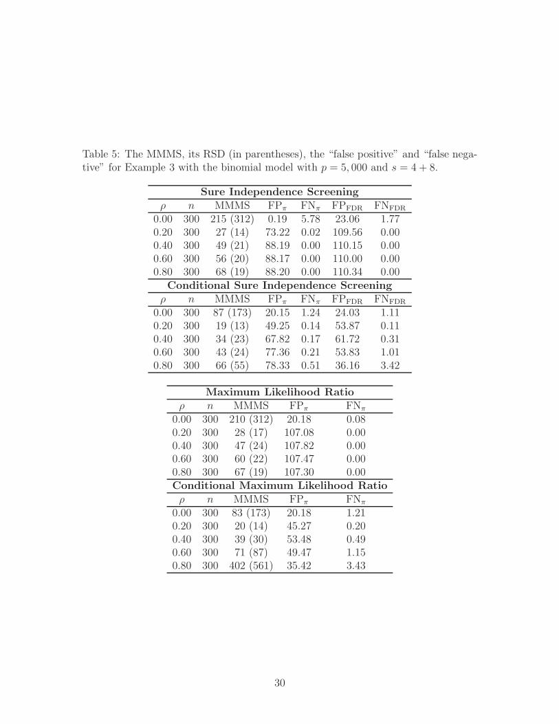
Table 5: The MMMS, its RSD (in parentheses), the “false positive” and “false nega-tive” for Example 3 with the binomial model with p = 5, 000 and s = 4 + 8.



0.00 300 215 (312) 0.19 5.78 23.06 1.770.20 300 27 (14) 73.22 0.02 109.56 0.000.40 300 49 (21) 88.19 0.00 110.15 0.000.60 300 56 (20) 88.17 0.00 110.00 0.000.80 300 68 (19) 88.20 0.00 110.34 0.00



0.00 300 87 (173) 20.15 1.24 24.03 1.110.20 300 19 (13) 49.25 0.14 53.87 0.110.40 300 34 (23) 67.82 0.17 61.72 0.310.60 300 43 (24) 77.36 0.21 53.83 1.010.80 300 66 (55) 78.33 0.51 36.16 3.42


ρ n MMMS FPπ FNπ


ρ n MMMS FPπ FNπ

0.00 300 83 (173) 20.18 1.210.20 300 20 (14) 45.27 0.200.40 300 39 (30) 53.48 0.490.60 300 71 (87) 49.47 1.150.80 300 402 (561) 35.42 3.43

30

Table 6: The MMMS, its RSD (in parentheses), the “false positive” and “false nega-tive” for Example 4 with the binomial model with p = 40, 000 and s = 2 + 4.



0.00 500 318 (7038) 12.04 1.22 51.32 0.790.20 500 38 (428) 32.47 0.57 68.46 0.380.40 500 38 (12) 38.66 0.27 73.42 0.190.60 500 38 (12) 41.99 0.16 76.11 0.100.80 500 35 (12) 43.84 0.03 77.38 0.02



0.00 500 13 (354) 5.96 0.66 42.51 0.490.20 500 15 (16) 14.51 0.39 49.79 0.270.40 500 16 (13) 19.11 0.24 51.68 0.220.60 500 19 (10) 22.80 0.21 51.78 0.240.80 500 19 (10) 26.39 0.14 46.49 0.64


ρ n MMMS FPπ FNπ

0.00 500 309 (7030) 14.06 0.220.20 500 37 (255) 34.10 0.090.40 500 35.5 (11) 40.50 0.050.60 500 35.5 (12) 42.89 0.030.80 500 33.5 (14) 44.39 0.00Conditional Maximum Likelihood Ratio

ρ n MMMS FPπ FNπ

0.00 500 25 (892) 5.96 0.140.20 500 13 (62) 12.38 0.090.40 500 13 (22) 14.17 0.080.60 500 15.5 (17) 13.75 0.110.80 500 22 (72) 9.30 0.28

31

5.2 Leukemia Data

In this section, we demonstrate how CSIS can be used to do variable selection with

an empirical dataset. We consider the leukemia dataset which was first studied by

Golub et al. (1999) and is available at http://www.broad.mit.edu/cgi-bin/cancer/datasets.cgi.

The data come from a study of gene expression in two types of acute leukemias, acute

lymphoblastic leukemia (ALL) and acute myeloid leukemia (AML). Gene expression

levels were measured using Affymetrix oligonucleotide arrays containing 7129 genes

and 72 samples coming from two classes, namely 47 in class ALL and 25 in class AML.

Among these 72 samples, 38 (27 ALL and 11 AML) are set to be training samples

and 34 (20 ALL and 14 AML) are set as test samples. For this dataset we want to se-

lect the relevant genes, and based on the selected genes estimate whether the patient

has ALL or AML. AML progresses very fast and has a poor prognosis. Therefore, a

consistent classification method that relies on gene expression levels would be very

beneficial for the diagnosis.

In order to choose the conditioning genes, we take a pair of genes described in

Golub et al. (1999) that result in low test errors. First is Zyxin and the second one

is Transcriptional activator hSNF2b. Both genes have empirically high correlations

for the difference between people with AML and ALL.

After conditioning on the aforementioned genes, we implement our conditional

selection procedure using logistic regression. Using the random decoupling method,

we select a single gene, TCRD (T-cell receptor delta locus). Although this gene has

not been discovered by the ALL/AML studies so far, it is known to have a relation

with T-Cell ALL, a subgroup of ALL (Szczepaski et al. 2003). By using only these

three genes, we are able to obtain a training error of 0 out of 38, and a test error

of 1 out of 34. Similar studies in the past using sparse linear discriminant analysis

or nearest shrunken centroids methods have obtained test errors of 1 by using more

32

http://www.broad.mit.edu/cgi-bin/cancer/datasets.cgi

than 10 variables. We conjecture that this is due to the high correlation between the

Zyxin gene and others, and that this correlation masks the information contained in

the TCRD gene.

5.3 Financial Data

In this section we illustrate the advantages of conditional sure independence screening

on a factor model with financial data. From the website http://mba.tuck.dartmouth.edu/pages

/faculty/ken.french/ we obtain 30 portfolios formed with respect to their industries.

The returns for each portfolio are denoted by yj (for j = 1, . . . 30). The Fama-French

three-factor model suggests that these returns follow the following equation

yji = bj1f1i + bj2f

2i + bj3f

3i + εi, (17)

where f 1 is the excess return of the proxy market portfolio (given by the difference

of the one-month T-Bill yield and the value weighted return of all stocks on NYSE,

AMEX and NASDAQ), f 2 is the difference between the return of small and big com-

panies (measured by the difference of returns of two portfolios, one with companies

that have small market cap and one with companies with large market cap) and fi-

nally f 3 is the difference of return from value companies and growth companies. This

model was first proposed by Fama and French (1993) and has been extensively ana-

lyzed since then. Since this seminal work, many other factors have been considered.

In our numerical example, we used screening with the permutation test to detect if

other factors are necessary. Besides the three factors mentioned above, we consider

the momentum factor as an additional factor. This gives us 4 factors that are condi-

tioned upon in CSIS. For each given industrial portfolio, we also consider the returns

from the other 29 portfolios as potential prediction factors.

33

We use daily returns data from 1/3/2002 to 12/31/2007. For each portfolio (30

in total), we first consider the marginal screening without conditioning. On average,

for each portfolio, marginal screening picks 25.3 among 29 other industrial portfolios

as predictors. This is mainly due to correlations between the returns of different

portfolios. We next consider conditional marginal screening, in which the three Fama-

French factors and the momentum factor are conditioned upon. As expected, the

number of the selected variables decreases significantly to an average of 4.8. That

is, about 4.8 portfolios on average can still have some potential prediction power in

presence of the aforementioned four major factors. The marginal and conditional fits

of the values are given in Figure 4. The black parts indicate the variables which are

not included.

It is seen from these results that, conditional screening is more advantageous

compared to marginal screening if few of the factors are known to be important. Fur-

thermore, when there is significant correlation between some of the factors, as shown

in the introduction, marginal screening considers most of the factors as relevant. In

almost all financial models, stock returns are correlated with the return of the market

portfolio. Therefore, in variable selection for financial factor models with many vari-

ables, one should always consider the returns conditional on the main driving forces

of the market.

APPENDIX

A.1 Proof of Theorem 1

Proof of Theorem 1. The necessary part has already been proven in Section 3.1. To

prove the sufficient condition, we first note that condition CovL(

Y,Xj

∣

∣XC

)

= 0 is

34

5

10

15

20

25

305 10 15 20 25 30

0

0.2

0.4

0.6

0.8

1

1.2

(a)∣

∣

∣βM

∣

∣

∣ using marginal screening

5 10 15 20 25 30

5

10

15

20

25

30

0.1

0.2

0.3

0.4

0.5

0.6

0.7

0.8

0.9

1

(b)∣

∣

∣βM

∣

∣

∣ using conditional screening

Figure 4: Chosen factors with marginal (left) and conditional screening (right).

equivalent to

E b′(XTCβ

MC )Xj = EY Xj ,

as shown in Section 3.1. This and (11) imply that ((βMC )T , 0)T is a solution to equation

(9). By the uniqueness, it follows that βMCj = ((βM

C )T , 0)T , namely βMj = 0. This

completes the proof.


Proof of Theorem 2. We denote the matrix EmjXCjXTCj as Ωj and partition it as

Ωj =

EmjXCXTC EmjXCXj

EmjXjXTC EmjX

2j

=

ΩC,C ΩC,j

ΩTC,j Ωj,j

.

From the score equations, i.e. equations (9) and (11), we have that

E b′(

XTCβ

MC

)

XC = E b′(

XTCjβ

MCj

)

XC.

35

Using the definition of mj , the above equation can be written as

Emj(XTCjβ

MCj −XT

CβMC )XC = 0.

By letting β∆,j = βMCj1 − βM

C , we have that

Emj(XTCβ

M∆,j +XT

j βMj )XC = 0.

or equivalently

β∆,j =− Ω−1C,CΩC,jβ

Mj . (A.1)

Furthermore, by (13), we can express CovL(Y,Xj|XC) as

CovL(Y,Xj|XC) = EXjY − EL(Y |XTC ). (A.2)

It follows from (12) that

CovL(Y,Xj|XC) = EXj

b′(

XTCjβ

MCj

)

− b′(

XTCβ

MC

)

. (A.3)

Using the definition of mj again, we have

CovL(Y,Xj|XC) = EmjXj(XTCjβ

MCj −XT

CβMC )

= EmjXj(XTCβ

M∆,j +XT

j βMj )

= ΩTC,jβ∆,j + Ωj,jβ

Mj .

By (A.1), we conclude that

CovL(Y,Xj|XC) = (Ωj,j − ΩTC,jΩ

−1C,CΩC,j)β

Mj . (A.4)

36

Now it is easy to see by Condition 1 that

|βMj | ≥ c−1

2 |CovL(Y,Xj|XC)| ≥ c3n−κ,

where c3 = c1/c2. Taking the minimum over all j ∈ MD⋆ gives the result.


The proof of Theorem 3 uses an exponential bound for a quasi maximum likelihood

estimator. This bound is shown in Fan and Song (2010) and we repeat their theorem

here to facilitate the reading.

Let β0 = argminβ El(XTβ, Y ) the population parameter, which is an interior

point of a large compact and convex set B ⊂ IRp.

Condition 5.

1. The Fisher information

I (β) = E

[

∂

∂βl(

XTβ, Y)

] [

∂

∂βl(

XTβ, Y)

]T

,

is finite and positive definite at β = β0. Furthermore, supβ∈B,x

∥

∥

∥I (β)1/2 x

∥

∥

∥/‖x‖

exists.

2. The function l(xTβ, y) is Lipschitz with a positive constant kn for any β in B,

and (x, y) in Λn = x, y : ‖x‖∞ ≤ Kn, |y| ≤ K⋆n with Kn and K⋆

n arbitrarily

large constants. Furthermore, there exists a constant C such that

supβ∈B,‖β−β

0‖≤CknV−1n (p/n)1/2

∣

∣E[

l(

XTβ, Y)

− l(

XTβ0, Y)]

(1− In (X, Y ))∣

∣ ≤ o (p/n) ,

(A.5)

37

where In (x, y) = I ((x, y) ∈ Λn) with constant Vn defined below.

3. The function l(

XTβ, Y)

is convex in β and

∣

∣E[

l(

XTβ, Y)

− l(

XTβ0, Y)]∣

∣ ≥ Vn ‖β − β0‖2 ,

for some positive constants Vn, and all ‖β − β0‖ ≤ CknV−1n (p/n)1/2.

Theorem 6. (Fan and Song 2010) Under Condition 5, for any t > 0 it holds that

P

(√n∥

∥

∥β − β0

∥

∥

∥≥ 16kn (1 + t) /Vn

)

≤ exp(

−2t2/K2n

)

+ nP (Λcn) .

The proof of Theorem 3 is based on Theorem 6.

Proof of Theorem 3. By Lemma 1 of Fan and Song (2010), Condition 2(ii) gives the

bound

P (|Y | ≥ u) ≤ s1 exp(−s0u).

Hence, we have

P(Λcn) ≤ P (‖X‖∞ > Kn) + P (|Y | ≥ K⋆

n) ≤ r2 exp(−r0Kαn ).

Using this and Theorem 6, letting 1 + t = c3Vnn1/2−κ/ (16kn), we have

P

(∣

∣

∣βMj − βM

j

∣

∣

∣≥ c3n

−κ)

≤ P

(∥

∥

∥β

M

Cj − βMCj

∥

∥

∥≥ c3n

−κ)

≤ exp(

−c4n1−2κ/ (knKn)

2)+ nr2 exp (−r0Kαn ) ,

for some positive constant c4. Then, by Bonferroni’s inequality, we obtain

P

(

maxq+1≤j≤p

∣

∣

∣βMj − βM

j

∣

∣

∣≥ c3n

−κ

)

≤ d(

exp(

−c4n1−2κ(knKn)

−2)

+nr2 exp(

−r0Kαn

)

)

.

38

This proves the first conclusion.

The second statement can be shown by considering the event

An =

maxj∈M⋆D

∣

∣

∣βMj − βM

j

∣

∣

∣≤ c3n

−κ/2

.

On the event An, by Theorem 2, it holds that for all j ∈ M⋆D

∣

∣

∣βMj

∣

∣

∣≥ c3n

−κ/2.

By letting γ = c5n−κ ≤ c3n

−κ/2, on the event An we have the sure screening property,

that is M⋆D ⊂ MD,γ. The probability bound can be shown by using the first result

along with Bonferroni’s inequality over all chosen j, which gives

P (Acn) ≤ s

[

exp(

−c4n1−2κ(knKn)

−2)

+ nr2 exp (−r0Kαn )]

.

This completes the proof.


Proof of Theorem 4. The first part of the proof is similar to that of Theorem 5 of

Fan and Song (2010). The idea of this proof is to show that

‖βD‖2 = O(

λmax

(

ΣD|C

))

. (A.6)

39

If this holds, the size of the set j = q + 1, . . . , p : |βMj | > εn−κ can not exceed

O(

n2κλmax

(

ΣD|C

))

for any ε > 0. Thus on the event

Bn =

maxq+1≤j≤p

|βMj − βM

j | ≤ εn−κ

,

the set j = q + 1, . . . , p : |βMj | > 2εn−κ is a subset of the set j = q + 1, . . . , p :

|βMj | > εn−κ, whose size is bounded by O

(

n2κλmax

(

ΣD|C

))

. If we take ε = c5/2, we

obtain that

P

(

|MD,γ| ≤ O(

n2κλmax

(

ΣD|C

))

)

≥ P(Bn).

Finally, by Theorem 3, we obtain that

P(Bn) ≥ 1− d(

exp(


−2)

+ nr2 exp(

− r0Kαn

)

)

and therefore the statement of the theorem follows.

We now prove (A.6) by using Var(XTβ⋆) = O(1) and (A.4). By Condition 3(ii),

the Schur’s complement (Ωj,j−ΩTC,jΩ

−1C,CΩC,j) is uniformly bounded from below. There-

fore, by (A.4), we have

|βMj | ≤ D1|CovL(Y,Xj |XC)|,

for a positive constant D1. Hence, we need only to bound the conditional covariance.

By (A.3), (9) and Lipschitz continuity of b′(·), we have

|CovL(Y,Xj|XC)| = E∣

∣Xj

b′(

XTβ∗)

− b′(

XTCβ

MC

)∣

∣

≤ D2 E∣

∣Xj(XTβ⋆ −XT

CβMC )

∣

∣

= D2 E∣

∣Xj [XTCβ

∆C +XT

Dβ⋆D]∣

∣.

40

where β∆C = (β⋆

C − βMC ). Writing the last term in the vector form, we need to bound

‖EXDXTDβ

⋆D +XDX

TCβ

∆C ‖2.

From the property of the least-squares, we have E[EL(XD|XC)XTC ] = E[XDX

TC ]. Thus

the above expression can be written as

‖[

ΣD|C

]

β⋆D + EEL(XD|XC)[X

TCβ

∆C + EL(X

TD|XC)β

∗D)]‖ =

∥

∥

[

ΣD|C

]

β⋆D + Z

∥

∥

2,

recalling the definition of Z = EEL(XD|XC)(

XTβ⋆ −XTCβ

MC

)

in Condition 3.

Using the law of total variance, we have that

∥

∥

[

ΣD|C

]

β⋆D + Z

∥

∥

2= β⋆

DT [ΣD|C

]2β⋆

D + 2ZT[

ΣD|C

]

+ ZTZ

≤ λmax

([

ΣD|C

])

(

β⋆DT [ΣD|C

]

β⋆D

)

+ 2ZT[

ΣD|C

]

+ ZTZ

≤ λmax

([

ΣD|C

])

Var(XTβ⋆) + 2ZT[

ΣD|C

]

+ ZTZ,

and the last two terms are o(

λmax

([

ΣD|C

]))

due to Condition 3. Therefore, we have

that

‖βD‖2 = O(

λmax

([

ΣD|C

]))

,

and that gives us the desired result.


Proof of Theorem 5. Note that the false discovery proportion can be rewritten as

E

∣

∣

∣MD,δ ∩ (M⋆D)

c∣

∣

∣

|(M⋆D)c|

=1

d− |M⋆D|∑

j∈(M⋆D)c

P

(

Ij

(

βMj

)1/2 ∣∣

∣βMj

∣

∣

∣≥ δ

)

.

41

With the given conditions, by Theorem 1, we have βMj = 0. Since XC includes the

intercept term, E ei = 0. It is known that Ij

(

βMj

)1/2 ∣∣

∣βMj

∣

∣

∣(for j ∈ (M⋆D)

c) has an

asymptotically standard normal distribution (Gao et al., 2008, Heyde, 1997). Then,

it follows that for a c7 > 0

supz

∣

∣

∣

∣

P

(

Ij

(

βMj

)1/2 ∣∣

∣βMj

∣

∣

∣≥ z

)

− Φ(z)

∣

∣

∣

∣

≤ c7n−1/2.

Combining both equations, we obtain

E

∣

∣

∣MD,δ ∩ (M⋆D)

c∣

∣

∣

|(M⋆D)c|

≤ 1

d− |M⋆D|∑

j∈(M⋆D)c

(

2 (1− Φ (δ)) + c7n−1/2

)

.

Setting δ = Φ−1(

1− f2d

)

gives the result.

References

Bickel, P.J., Ritov, Y., and Tsybakov, A.B. (2009), “Simultaneous Analysis of Lasso

and Dantzig selector,” The Annals of Statistics, 37 1705–1732.

Buhlmann, P., and van de Geer, S. (2011), Statistics for High-Dimensional Data:

Methods, Theory and Applications, New York: Springer.

Candes, E., and Tao, T. (2007), “The Dantzig Selector: Statistical Estimation When

p Is Much Larger Than n” (with discussion), The Annals of Statistics, 35, 2313–

2351.

Efron B., Hastie T., Johnstone I., and Tibshirani R. (2004), “Least Angle Regression,”

The Annals of Statistics, 32, 407–499.

42

Fama, E.F., and French, K.R. (1993), “Common Risk Factors in the Returns on

Stocks and Bonds,” Journal of Financial Economics, 33, 3–56.

Fan, J., Feng, Y., and Song, R. (2011), “Nonparametric Independence Screening in

Sparse Ultra-High-Dimensional Additive Models,” Journal of the American Statis-

tical Association, 106, 544–557.

Fan, J., and Li, R. (2001), “Variable Selection via Nonconcave Penalized Likelihood

and its Oracle Properties,” Journal of the American Statistical Association, 96,

1348–1360.

Fan, J., and Lv, J. (2008), “Sure Independence Screening for Ultrahigh Dimen-

sional Feature Space,” Journal of the Royal Statistical Society: Series B (Statistical

Methodology), 70, 849–911.

Fan, J., and Lv, J. (2011), “Nonconcave Penalized Likelihood With NP-

Dimensionality,” Information Theory, IEEE Transactions, 57, 5467–5484.

Fan, J., Samworth, R., and Wu, Y. (2009), “Ultrahigh Dimensional Feature Selection:

Beyond the Linear Model,” The Journal of Machine Learning Research, 10, 2013–

2038.

Fan, J., and Song, R. (2010), “Sure Independence Screening in Generalized Linear

Models with NP-dimensionality,” The Annals of Statistics, 38, 3567–3604.

Frank, I.E., and Friedman, J. (1993), “A Statistical View of Some Chemometrics

Regression Tools,” Technometrics, 35, 109–135.

Gao, Q., Wu, Y., Zhu, C. and Wang, Z. (2008), “Asymptotic Normality of Maximum

Quasi-Likelihood Estimators in Generalized Linear Models with Fixed Design,”

Journal of Systems Science and Complexity, 21, 463–473.

43

Golub, T., Slonim, D., Tamayo, P., Huard, C., Gaasenbeek, M., Mesirov, J., Coller,

H., Loh, M., Downing, J., Caligiuri, M., Bloomfield, C., and Lander, E. (1999),

“Molecular Classification of Cancer: Class Discovery and Class Prediction by Gene

Expression Monitoring,” Science, 286, 531–537.

Hall, P., and Miller, H. (2009), “Using Generalized Correlation to Effect Variable

Selection in Very High Dimensional Problems,” Journal of Computational and

Graphical Statistics, 18, 533–550.

Hastie, T.J., Tibshirani, R., and Friedman, J. (2009), The Elements of Statistical

Learning: Data Mining, Inference and Prediction, New York: Springer.

Hall, P., Titterington, D.M., and Xue, J. H. (2009), “Tilting Methods for Assess-

ing the Influence of Components in a Classifier,” Journal of the Royal Statistical

Society: Series B (Statistical Methodology), 71, 783–803.

Heyde, C.C. (1997), Quasi-likelihood and its Application: a General Approach to

Optimal Parameter Estimation, New York: Springer.

Li, G., Peng, H., Zhang, J., and Zhu, L. (2012), “Robust Sure Independence Screening

Based on Rank Correlation for the Ultrahigh Dimensional Models,” manuscript,

Beijing University of Technology.

Osborne, M.R., Presnell, B. and Turlach, B.A. (2000a), “On the LASSO and its

Dual,” Journal of Computational and Graphical Statistics, 9, 319–337.

Osborne, M.R., Presnell, B. and Turlach, B.A. (2000b), “A New Approach to Variable

Selection in Least Squares Problems,” IMA Journal of Numerical Analysis, 20,

389–403.

Szczepaski, T., van der Velden, V.H., Raff, T., Jacobs, D.C., van Wering, E.R.,

Brggemann, M., Kneba, M., and van Dongen, J.J. (2003), “Comparative Anal-

44

ysis of T-cell Receptor Gene Rearrangements at Diagnosis and Relapse of T-cell

Acute Lymphoblastic Leukemia (T-ALL) Shows High Stability of Clonal Markers

for Monitoring of Minimal Residual Disease and Reveals the Occurrence of Second

T-ALL,” Leukemia, 17, 2149–2156.

Tibshirani, R. (1996), “Regression Shrinkage and Selection via the Lasso,” Journal

of the Royal Statistical Society: Series B (Statistical Methodology), 58, 267–288.

Wasserman, L., and Roeder, K. (2009), “High-dimensional Variable Selection,” The

Annals of Statistics, 37, 2178–2201.

Zhang, C., and Zhang, T. (2012), “A General Theory of Concave Regularization for

High Dimensional Sparse Estimation Problems,” manuscript, Rutgers University.

Zhao, S.D., and Li, Y. (2012), “Principled Sure Independence Screening for Cox Mod-

els with Ultra-high Dimensional Covariates,” Journal of Multivariate Analysis, 105,

397–411.

45

conditional sure independence screening - arxiv · of variables. this results in conditional sure...

Documents