on over-fitting in model selection and subsequent selection bias in

Journal of Machine Learning Research 11 (2010) 2079-2107 Submitted 10/09; Revised 3/10; Published 7/10

On Over-fitting in Model Selection and Subsequent Selection Bias inPerformance Evaluation

Gavin C. Cawley [email protected]

Nicola L. C. Talbot [email protected]

School of Computing SciencesUniversity of East AngliaNorwich, United Kingdom NR4 7TJ

Editor: Isabelle Guyon

Abstract

Model selection strategies for machine learning algorithms typically involve the numerical opti-misation of an appropriate model selection criterion, often based on an estimator of generalisationperformance, such ask-fold cross-validation. The error of such an estimator can be broken downinto bias and variance components. While unbiasedness is often cited as a beneficial quality of amodel selection criterion, we demonstrate that a low variance is at least as important, as a non-negligible variance introduces the potential for over-fitting in model selection as well as in trainingthe model. While this observation is in hindsight perhaps rather obvious, the degradation in perfor-mance due to over-fitting the model selection criterion can be surprisingly large, an observation thatappears to have received little attention in the machine learning literature to date. In this paper, weshow that the effects of this form of over-fitting are often ofcomparable magnitude to differencesin performance between learning algorithms, and thus cannot be ignored in empirical evaluation.Furthermore, we show that some common performance evaluation practices are susceptible to aform of selection bias as a result of this form of over-fittingand hence are unreliable. We dis-cuss methods to avoid over-fitting in model selection and subsequent selection bias in performanceevaluation, which we hope will be incorporated into best practice. While this study concentrateson cross-validation based model selection, the findings arequite general and apply to any modelselection practice involving the optimisation of a model selection criterion evaluated over a finitesample of data, including maximisation of the Bayesian evidence and optimisation of performancebounds.

Keywords: model selection, performance evaluation, bias-variance trade-off, selection bias, over-fitting

1. Introduction

This paper is concerned with two closely related topics that form core components of best practice inboth the real world application of machine learning methods and the development of novel machinelearning algorithms, namely model selection and performance evaluation. Themajority of machinelearning algorithms are based on some form of multi-level inference, wherethe model is definedby a set of model parameters and also a set of hyper-parameters (Guyon et al., 2009), for examplein kernel learning methods the parameters correspond to the coefficients of the kernel expansionand the hyper-parameters include the regularisation parameter, the choiceof kernel function andany associated kernel parameters. This division into parameters and hyper-parameters is typically

c©2010 Gavin C. Cawley and Nicola L. C. Talbot.

CAWLEY AND TALBOT

performed for computational convenience; for instance in the case of kernel machines, for fixedvalues of the hyper-parameters, the parameters are normally given by thesolution of a convexoptimisation problem for which efficient algorithms are available. Thus it makessense to takeadvantage of this structure and fit the model iteratively using a pair of nested loops, with the hyper-parameters adjusted to optimise a model selection criterion in the outer loop (modelselection) andthe parameters set to optimise a training criterion in the inner loop (model fitting/training). Inour previous study (Cawley and Talbot, 2007), we noted that the variance of the model selectioncriterion admitted the possibility of over-fitting during model selection as well as the more familiarform of over-fitting that occurs during training and demonstrated that this could be ameliorated tosome extent by regularisation of the model selection criterion. The first part of this paper discussesthe problem of over-fitting in model selection in more detail, providing illustrativeexamples, anddescribes how to avoid this form of over-fitting in order to gain the best attainable performance,desirable in practical applications, and required for fair comparison of machine learning algorithms.

Unbiased and robust1 performance evaluation is undoubtedly the cornerstone of machine learn-ing research; without a reliable indication of the relative performance of competing algorithms,across a wide range of learning tasks, we cannot have the clear pictureof the strengths and weak-nesses of current approaches required to set the direction for future research. This topic is consid-ered in the second part of the paper, specifically focusing on the undesirable optimistic bias thatcan arise due to over-fitting in model selection. This phenomenon is essentiallyanalogous to theselection bias observed by Ambroise and McLachlan (2002) in microarrayclassification, due tofeature selection prior to performance evaluation, and shares a similar solution. We show that some,apparently quite benign, performance evaluation protocols in common use bythe machine learningcommunity are susceptible to this form of bias, and thus potentially give spurious results. In orderto avoid this bias, model selection must be treated as an integral part of the model fitting process andperformed afresh every time a model is fitted to a new sample of data. Furthermore, as the differ-ences in performance due to model selection are shown to be often of comparable magnitude to thedifference in performance between learning algorithms, it seems no longer meaningful to evaluatethe performance of machine learning algorithms in isolation, and we should instead compare learn-ing algorithm/model selection procedure combinations. However, this means that robust unbiasedperformance evaluation is likely to require more rigorous and computationally intensive protocols,such a nested cross-validation or “double cross” (Stone, 1974).

None of the methods or algorithms discussed in this paper are new; the novelcontributionof this work is an empirical demonstration that over-fitting at the second levelof inference (i.e.,model selection) can have a very substantial deleterious effect on the generalisation performance ofstate-of-the-art machine learning algorithms. Furthermore the demonstrationthat this can lead to amisleading optimistic bias in performance evaluation using evaluation protocols in common use inthe machine learning community is also novel. The paper is intended to be of some tutorial value inpromoting best practice in model selection and performance evaluation, however we also hope thatthe observation that over-fitting in model selection is a significant problem willencourage muchneeded algorithmic and theoretical development in this area.

The remainder of the paper is structured as follows: Section 2 provides a brief overview of thekernel ridge regression classifier used as the base classifier for the majority of the experimental work

1. The term “robust” is used here to imply insensitivity to irrelevant experimental factors, such as the sampling and par-titioning of the data to form training, validation and test sets; this is normally achieved by computationally expensiveresampling schemes, for example, cross-validation (Stone, 1974) and the bootstrap (Efron and Tibshirani, 1994).

2080

OVERFITTING IN MODEL SELECTION AND SELECTION BIAS IN PERFORMANCEEVALUATION

and Section 3 describes the data sets used. Section 4 demonstrates the importance of the varianceof the model selection criterion, as it can lead to over-fitting in model selection,resulting in poorgeneralisation performance. A number of methods to avoid over-fitting in model selection are alsodiscussed. Section 5 shows that over-fitting in model selection can result inbiased performanceevaluation if model selection is not viewed as an integral part of the modelling procedure. Twoapparently benign and widely used performance evaluation protocols areshown to be affected bythis problem. Finally, the work is summarised in Section 6.

2. Kernel Ridge Regression

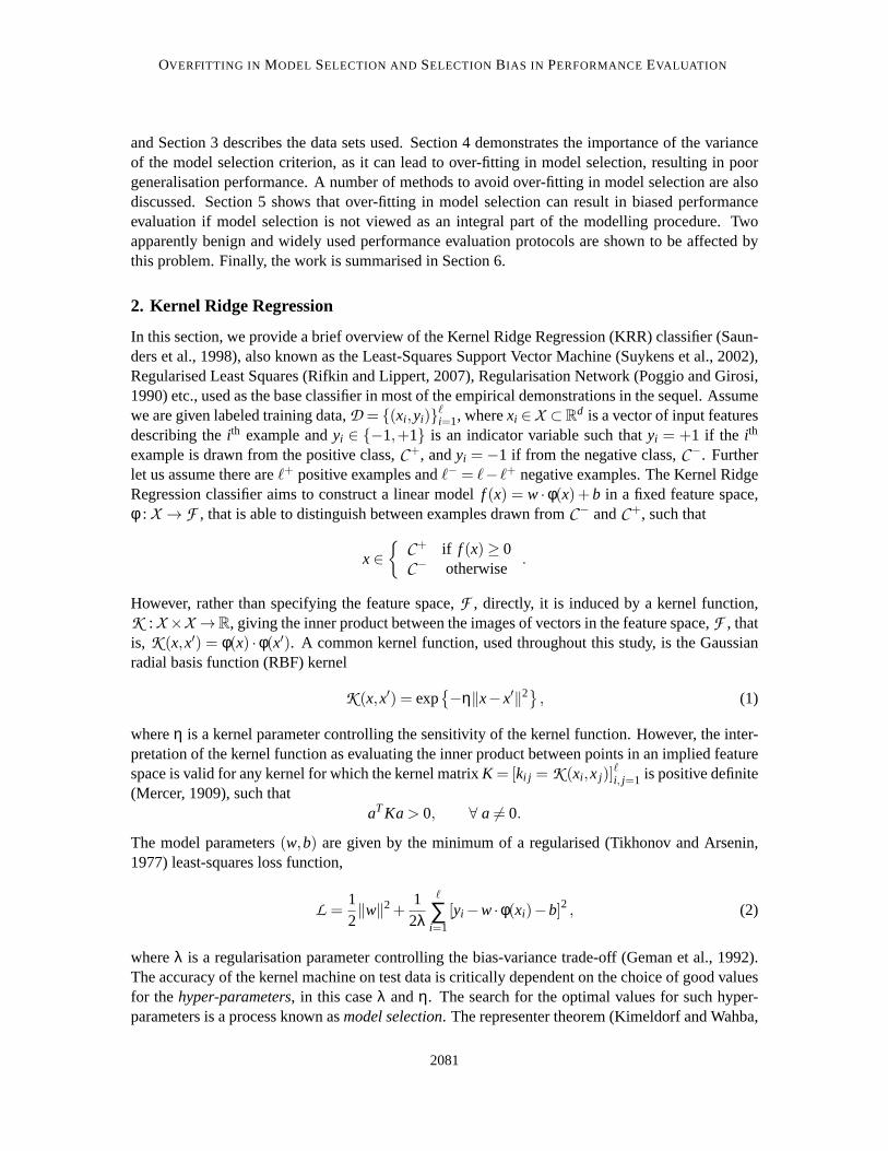
In this section, we provide a brief overview of the Kernel Ridge Regression (KRR) classifier (Saun-ders et al., 1998), also known as the Least-Squares Support Vector Machine (Suykens et al., 2002),Regularised Least Squares (Rifkin and Lippert, 2007), RegularisationNetwork (Poggio and Girosi,1990) etc., used as the base classifier in most of the empirical demonstrations inthe sequel. Assumewe are given labeled training data,D = {(xi ,yi)}

ℓi=1, wherexi ∈ X ⊂R

d is a vector of input featuresdescribing theith example andyi ∈ {−1,+1} is an indicator variable such thatyi = +1 if the ith

example is drawn from the positive class,C+, andyi = −1 if from the negative class,C−. Furtherlet us assume there areℓ+ positive examples andℓ− = ℓ− ℓ+ negative examples. The Kernel RidgeRegression classifier aims to construct a linear modelf (x) = w · φ(x)+b in a fixed feature space,φ : X → F , that is able to distinguish between examples drawn fromC− andC+, such that

x∈

{

C+ if f (x)≥ 0C− otherwise

.

However, rather than specifying the feature space,F , directly, it is induced by a kernel function,K : X ×X →R, giving the inner product between the images of vectors in the feature space,F , thatis, K (x,x′) = φ(x) ·φ(x′). A common kernel function, used throughout this study, is the Gaussianradial basis function (RBF) kernel

K (x,x′) = exp{

−η‖x−x′‖2} , (1)

whereη is a kernel parameter controlling the sensitivity of the kernel function. However, the inter-pretation of the kernel function as evaluating the inner product between points in an implied featurespace is valid for any kernel for which the kernel matrixK = [ki j =K (xi ,x j)]

ℓi, j=1 is positive definite

(Mercer, 1909), such thataTKa> 0, ∀ a 6= 0.

The model parameters(w,b) are given by the minimum of a regularised (Tikhonov and Arsenin,1977) least-squares loss function,

L =12‖w‖2+

12λ

ℓ

∑i=1

[yi −w·φ(xi)−b]2 , (2)

whereλ is a regularisation parameter controlling the bias-variance trade-off (Geman et al., 1992).The accuracy of the kernel machine on test data is critically dependent onthe choice of good valuesfor thehyper-parameters, in this caseλ andη. The search for the optimal values for such hyper-parameters is a process known asmodel selection. The representer theorem (Kimeldorf and Wahba,

2081

CAWLEY AND TALBOT

1971) states that the solution to this optimisation problem can be written as an expansion of theform

w=ℓ

∑i=1

αiφ(xi) =⇒ f (x) =ℓ

∑i=1

αiK (xi ,x)+b.

The dual parameters of the kernel machine,α, are then given by the solution of a system of linearequations,

[

K+λI 11T 0

][

αb

]

=

[

y0

]

. (3)

wherey = (y1,y2, . . . ,yℓ)T , which can be solved efficiently via Cholesky factorisation ofK + λI ,with a computational complexity ofO(ℓ3) operations (Suykens et al., 2002). The simplicity andefficiency of the kernel ridge regression classifier makes it an ideal candidate for relatively small-scale empirical investigations of practical issues, such as model selection.

2.1 Efficient Leave-One-Out Cross-Validation

Cross-validation (e.g., Stone, 1974) provides a simple and effective methodfor both model selec-tion and performance evaluation, widely employed by the machine learning community. Underk-fold cross-validation the data are randomly partitioned to formk disjoint subsets of approximatelyequal size. In theith fold of the cross-validation procedure, theith subset is used to estimate thegeneralisation performance of a model trained on the remainingk− 1 subsets. The average ofthe generalisation performance observed over allk folds provides an estimate (with a slightly pes-simistic bias) of the generalisation performance of a model trained on the entiresample. The mostextreme form of cross-validation, in which each subset contains only a single pattern is known asleave-one-out cross-validation (Lachenbruch and Mickey, 1968; Luntz and Brailovsky, 1969). Anattractive feature of kernel ridge regression is that it is possible to perform leave-one-out cross-validation in closed form, with minimal cost as a by-product of the training algorithm (Cawley andTalbot, 2003). LetC represent the matrix on the left hand side of (3), then the residual errorfor theith training pattern in theith fold of the leave-one-out process is given by,

r(−i)i = yi − y(−i)

i =αi

C−1ii

,

wherey(− j)i is the output of the kernel ridge regression machine for theith observation in thej th fold

of the leave-one-out procedure andC−1ii is the ith element of the principal diagonal of the inverse

of the matrixC. Similar methods have been used in least-squares linear regression for many years,(e.g., Stone, 1974; Weisberg, 1985). While the optimal model parameters ofthe kernel machineare given by the solution of a simple system of linear equations, (3), some form of model selectionis required to determine good values for thehyper-parameters, θ = (λ,η), in order to maximisegeneralisation performance. The analytic leave-one-out cross-validation procedure described herecan easily be adapted to form the basis of an efficient model selection strategy (cf. Chapelle et al.,2002; Cawley and Talbot, 2003; Bo et al., 2006). In order to obtain a continuous model selectioncriterion, we adopt Allen’s Predicted REsidual Sum-of-Squares (PRESS) statistic (Allen, 1974),

PRESS(θ) =ℓ

∑i=1

[

r(−i)i

]2.

2082


The PRESS criterion can be optimised efficiently using scaled conjugate gradient descent (Williams,1991) or Nelder-Mead simplex (Nelder and Mead, 1965) procedures.For full details of the train-ing and model selection procedures for the kernel ridge regression classifier, see Cawley (2006).A public domain MATLAB implementation of the kernel ridge regression classifier, including au-tomated model selection, is provided by the Generalised Kernel Machine (GKM) (Cawley et al.,2007) toolbox.2

3. Data Sets used in Empirical Demonstrations

In this section, we describe the benchmark data sets used in this study to illustrate the problemof over-fitting in model selection and to demonstrate the bias this can introduce into performanceevaluation.

3.1 A Synthetic Benchmark

A synthetic benchmark, based on that introduced by Ripley (1996), is used widely in the nextsection to illustrate the nature of over-fitting in model selection. The data are drawn from fourspherical bivariate Gaussian distributions, with equal probability. All four Gaussians have a com-mon variance,σ2 = 0.04. Patterns belonging to the positive classes are drawn from Gaussianscentered on[+0.4,+0.7] and [−0.3,+0.7]; the negative patterns are drawn from Gaussians cen-tered on[−0.7,+0.3] and [+0.3,+0.3]. Figure 1 shows a realisation of the synthetic benchmark,consisting of 256 patterns, showing the Bayes-optimal decision boundaryand contours representingan a-posteriori probability of belonging to the positive class of 0.1 and 0.9. The Bayes error forthis benchmark is approximately 12.38%. This benchmark is useful firstly as the Bayes optimaldecision boundary is known, but also because it provides an inexhaustible supply of data, allowingthe numerical approximation of various expectations.

3.2 A Suite of Benchmarks for Robust Performance Evaluation

In addition to illustrating the nature of over-fitting in model selection, we need to demonstrate thatit is a serious concern in practical applications and show that it can resultin biased performanceevaluation if not taken into consideration. Table 1 gives the details of a suite of thirteen benchmarkdata sets, introduced by Ratsch et al. (2001). Each benchmark is based on a data set from theUCI machine learning repository, augmented by a set of 100 pre-definedpartitions to form multiplerealisations of the training and test sets (20 in the case of the largerimage andsplice data sets).The use of multiple benchmarks means that the evaluation is more robust as the selection of datasets that provide a good match to the inductive bias of a particular classifier becomes less likely.Likewise, the use of multiple partitions provides robustness against sensitivity to the sampling ofdata to form training and test sets. Results on this suite of benchmarks thus provides a reasonableindication of the magnitude of the effects of over-fitting in model selection that we might expect tosee in practice.

2. Toolbox can be found athttp://theoval.cmp.uea.ac.uk/ ˜ gcc/projects/gkm .

2083

CAWLEY AND TALBOT

x1

x 2

−1.5 −1 −0.5 0 0.5 1−0.5

0

0.5

1

1.5

p(C+|x) = 0.9

p(C+|x) = 0.5

p(C+|x) = 0.1

x1

x 2

−1.5 −1 −0.5 0 0.5 1−0.5

0

0.5

1

1.5

f(x) = +1f(x) = 0f(x) = −1

(a) (b)

Figure 1: Realisation of the Synthetic benchmark data set, with Bayes optimal decision bound-ary (a) and kernel ridge regression classifier with an automatic relevance determination(ARD) kernel where the hyper-parameters are tuned so as to minimise the true test MSE(b).

Data SetTraining Testing Number of InputPatterns Patterns Replications Features

banana 400 4900 100 2breast cancer 200 77 100 9diabetis 468 300 100 8flare solar 666 400 100 9german 700 300 100 20heart 170 100 100 13image 1300 1010 20 18ringnorm 400 7000 100 20splice 1000 2175 20 60thyroid 140 75 100 5titanic 150 2051 100 3twonorm 400 7000 100 20waveform 400 4600 100 21

Table 1: Details of data sets used in empirical comparison.

4. Over-fitting in Model Selection

We begin by demonstrating that it is possible to over-fit a model selection criterion based on a finitesample of data, using the synthetic benchmark problem, where ground truth isavailable. Here weuse “over-fitting in model selection” to mean minimisation of the model selection criterion beyondthe point at which generalisation performance ceases to improve and subsequently begins to decline.

2084


Figure 1 (b) shows the output of a kernel ridge regression classifier for the synthetic problem, withthe Automatic Relevance Determination (ARD) variant of the Gaussian radial basis function kernel,

K (x,x′) = exp

{

−d

∑i=1

ηi(xi −x′i)2

}

,

which has a separate scaling parameter,ηi , for each feature. A much larger training set of 4096samples was used, and the hyper-parameters were tuned to minimise the true test mean squarederrors (MSE). The performance of this model achieved an error rate of 12.50%, which suggests thata model of this form is capable of approaching the Bayes error rate for this problem, at least inprinciple, and so there is little concern of model mis-specification.

0 20 40 60 80 1000.2

0.205

0.21

0.215

0.22

0.225

0.23

iteration

MS

E

X−Validation

Test

0 20 40 60 80 1000.2

0.21

0.22

0.23

0.24

0.25

0.26

0.27

iteration

MS

E

X−Validation

Test

(a) (b)

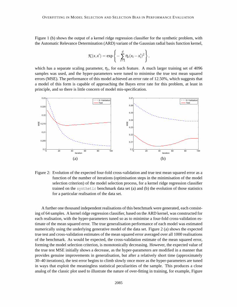
Figure 2: Evolution of the expected four-fold cross-validation and true test mean squared error as afunction of the number of iterations (optimisation steps in the minimisation of the modelselection criterion) of the model selection process, for a kernel ridge regression classifiertrained on thesynthetic benchmark data set (a) and (b) the evolution of those statisticsfor a particular realisation of the data set.

A further one thousand independent realisations of this benchmark weregenerated, each consist-ing of 64 samples. A kernel ridge regression classifier, based on the ARD kernel, was constructed foreach realisation, with the hyper-parameters tuned so as to minimise a four-foldcross-validation es-timate of the mean squared error. The true generalisation performance of each model was estimatednumerically using the underlying generative model of the data set. Figure 2 (a) shows the expectedtrue test and cross-validation estimates of the mean squared error averaged over all 1000 realisationsof the benchmark. As would be expected, the cross-validation estimate of themean squared error,forming the model selection criterion, is monotonically decreasing. However,the expected value ofthe true test MSE initially shows a decrease, as the hyper-parameters are modified in a manner thatprovides genuine improvements in generalisation, but after a relatively short time (approximately30–40 iterations), the test error begins to climb slowly once more as the hyper-parameters are tunedin ways that exploit the meaningless statistical peculiarities of the sample. This produces a closeanalog of the classic plot used to illustrate the nature of over-fitting in training,for example, Figure

2085

CAWLEY AND TALBOT

9.7 of the book by Bishop (1995). Figure 2 (b) shows the same statistics forone particular realisationof the data, demonstrating that the over-fitting can in some cases be quite substantial, clearly in thiscase some form of early-stopping in the model selection process would have resulted in improvedgeneralisation. Having demonstrated that the classic signature of over-fitting during training is alsoapparent in the evolution of cross-validation and test errors during model selection, we discuss inthe next section the origin of this form of over-fitting in terms of thebiasandvarianceof the modelselection criterion.

4.1 Bias and Variance in Model Selection

Model selection criteria are generally based on an estimator of generalisation performance evaluatedover a finite sample of data, this includes resampling methods, such as split sample estimators,cross-validation (Stone, 1974) and bootstrap methods (Efron and Tibshirani, 1994), but also moreloosely, the Bayesian evidence (MacKay, 1992; Rasmussen and Williams, 2006) and theoreticalperformance bounds such as the radius-margin bound (Vapnik, 1998). The error of an estimator canbe decomposed into two components,biasandvariance. Let G(θ) represent the true generalisationperformance of a model with hyper-parametersθ, andg(θ;D) be an estimate of generalisationperformance evaluated over a finite sample,D, of n patterns. The expected squared error of theestimator can then be written in the form (Geman et al., 1992; Duda et al., 2001),

ED

{

[g(θ;D)−G(θ)]2}

= [ED {g(θ;D)−G(θ)}]2+ ED

{

[

g(θ;D)−ED ′

{

g(θ;D ′)}]2

}

,

whereED{·} represents an expectation evaluated over independent samples,D, of sizen. The firstterm, the squaredbias, represents the difference between the expected value of the estimator and theunknown value of the true generalisation error. The second term, knownas thevariance, reflectsthe variability of the estimator around its expected value due to the sampling of the dataD onwhich it is evaluated. Clearly if the expected squared error is low, we may reasonably expectg(·) toperform well as a model selection criterion. However, in practice, the expected squared error maybe significant, in which case, it is interesting to ask whether the bias or the variance component isof greatest importance in reliably achieving optimal generalisation.

It is straightforward to demonstrate that leave-one-out cross-validationprovides an almost un-biased estimate of the true generalisation performance (Luntz and Brailovsky, 1969), and this isoften cited as being an advantageous property of the leave-one-out estimator in the setting of modelselection (e.g., Vapnik, 1998; Chapelle et al., 2002). However, for the purpose of model selection,rather than performance evaluation, unbiasednessper seis relatively unimportant, instead the pri-mary requirement is merely for the minimum of the model selection criterion to provide a reliableindication of the minimum of the true test error in hyper-parameter space. Thispoint is illustratedin Figure 3, which shows a hypothetical example of a model selection criterionthat is unbiased (byconstruction) (a) and another that is clearly biased (b). Unbiasednessprovides the assurance thatthe minimum of the expected value of the model selection criterion,ED{g(θ;D)} coincides withthe minimum of the test error,G(θ). However, in practice, we have only a finite sample of data,Di ,over which to evaluate the model selection criterion, and so it is the minimum ofg(θ;Di) that is ofinterest. In Figure 3 (a), it can be seen that while the estimator is unbiased, ithas a high variance,and so there is a large spread in the values ofθ at which the minimum occurs for different samplesof data, and sog(θ;Di) is likely to provide a poor model selection criterion in practice. On the otherhand, Figure 3 (b) shows a criterion with lower variance, and hence is thebetter model selection

2086


criterion, despite being biased, as the minima ofg′(θ;Di) for individual samples lie much closerto the minimum of the true test error. This demonstrates that while unbiasednessis reassuring, asit means that the form of the model selection criterion is correcton average, the variance of thecriterion is also vitally important as it is this that ensures that the minimum of the selection criterionevaluated on a particular sample will provide good generalisation.

0 2 4 6 8 100

0.2

0.4

0.6

0.8

1

err

or

rate

θ

test errorE

Dg(θ;D)

g(θ;Di)

0 2 4 6 8 100

0.2

0.4

0.6

0.8

1

err

or

rate

θ

test errorE

Dg’(θ;D)

g’(θ;Di)

(a) (b)

Figure 3: Hypothetical example of an unbiased (a) and a biased (b) modelselection criterion. Notethat the biased model selection criterion (b) is likely to provide the more effective modelselection criterion as it has a lower variance, even though it is significantly biased. Forclarity, the true error rate and the expected value of the model selection criteria are shownwith vertical displacements of−0.6 and−0.4 respectively.

4.2 The Effects of Over-fitting in Model Selection

In this section, we investigate the effect of the variance of the model selection criterion using amore realistic example, again based on thesynthetic benchmark, where the underlying generativemodel is known and so we are able to evaluate the true test error. It is demonstrated that over-fittingin model selection can cause both under-fitting and over-fitting of the trainingsample. A fixedtraining set of 256 patterns is generated and used to train a kernel ridge regression classifier, usingthe simple RBF kernel (1), with hyper-parameter settings defining a fine gridspanning reasonablevalues of the regularisation and kernel parameters,λ andη respectively. The smoothed error rate(Bo et al., 2006),

SER(θ) =12n

n

∑i=1

[1−yi tanh{γ f (xi)}]

is used as the statistic of interest, in order to improve the clarity of the figures, whereγ is a param-eter controlling the amount of smoothing applied (γ = 8 is used throughout, however the precisevalue is not critical). Figure 4 (a) shows the true test smoothed error rate as a function of the hyper-parameters. As these are both scale parameters, a logarithmic representation is used for both axes.The true test smoothed error rate is an approximately unimodal function of thehyper-parameters,

2087

CAWLEY AND TALBOT

with a single distinct minimum, indicating the hyper-parameter settings giving optimal generalisa-tion.

log2η

log

2λ

−8 −6 −4 −2 0 2 4 6 8

−10

−8

−6

−4

−2

0

2

4

6

8

log2η

log

2λ

−8 −6 −4 −2 0 2 4 6 8

−10

−8

−6

−4

−2

0

2

4

6

8

(a) (b)

Figure 4: Plot of the true test smoothed error rate (a) and mean smoothed error rate over 100 randomvalidation sets of 64 samples (b), for a kernel ridge regression classifier as a function ofthe hyper-parameters. In each case, the minimum is shown by a yellow cross, +.

In practical applications, however, the true test error is generally unknown, and so we must relyon an estimator of some sort. The simplest estimator for use in model selection is theerror computedover an independent validation set, that is, the split-sample estimator. It seemsentirely reasonableto expect the split-sample estimator to be unbiased. Figure 4 (b) shows a plot of the mean smoothederror rate using the split-sample estimator, over 100 random validation sets, each of which consistsof 64 patterns. Note that the same fixed training set is used in each case. This plot is very similarto the true smoothed error, shown in Figure 4 (a), demonstrating that the splitsample estimator isindeed approximately unbiased.

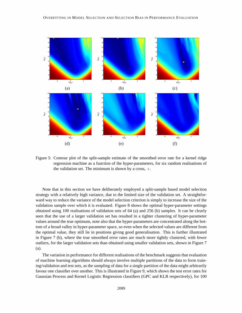
While the split-sample estimator is unbiased, it may have a high variance, especially as in thiscase the validation set is (intentionally) relatively small. Figure 5 shows plots ofthe split-sampleestimate of the smoothed error rate for six selected realisations of a validation set of 64 patterns.Clearly, the split-sample error estimate is no longer as smooth, or indeed unimodal. More impor-tantly, the hyper-parameter values selected by minimising the validation set error, and therefore thetrue generalisation performance, depends on the particular sample of dataused to form the valida-tion set. Figure 6 shows that the variance of the split-sample estimator can result in models rangingfrom severely under-fit (a) to severely over-fit (f), with variations inbetween these extremes.

Figure 7 (a) shows a scatter plot of the validation set and true error ratesfor kernel ridge re-gression classifiers for the synthetic benchmark, with split-sample based model selection using 100random realisations of the validation set. Clearly, the split-sample based modelselection procedurenormally performs well. However, there is also significant variation in performance with differentsamples forming the validation set. We can also see that the validation set erroris strongly biased,having been directly minimised during model selection, and (of course) should not be used forperformance estimation.

2088


log2η

log

2λ

−5 0 5

−10

−8

−6

−4

−2

0

2

4

6

8

log2η

log

2λ

−5 0 5

−10

−8

−6

−4

−2

0

2

4

6

8

log2η

log

2λ

−5 0 5

−10

−8

−6

−4

−2

0

2

4

6

8

(a) (b) (c)

log2η

log

2λ

−5 0 5

−10

−8

−6

−4

−2

0

2

4

6

8

log2η

log

2λ

−5 0 5

−10

−8

−6

−4

−2

0

2

4

6

8

log2η

log

2λ

−5 0 5

−10

−8

−6

−4

−2

0

2

4

6

8

(d) (e) (f)

Figure 5: Contour plot of the split-sample estimate of the smoothed error rate for a kernel ridgeregression machine as a function of the hyper-parameters, for six random realisations ofthe validation set. The minimum is shown by a cross,+.

Note that in this section we have deliberately employed a split-sample based model selectionstrategy with a relatively high variance, due to the limited size of the validation set.A straightfor-ward way to reduce the variance of the model selection criterion is simply to increase the size of thevalidation sample over which it is evaluated. Figure 8 shows the optimal hyper-parameter settingsobtained using 100 realisations of validation sets of 64 (a) and 256 (b) samples. It can be clearlyseen that the use of a larger validation set has resulted in a tighter clusteringof hyper-parametervalues around the true optimum, note also that the hyper-parameters are concentrated along the bot-tom of a broad valley in hyper-parameter space, so even when the selected values are different fromthe optimal value, they still lie in positions giving good generalisation. This is further illustratedin Figure 7 (b), where the true smoothed error rates are much more tightly clustered, with feweroutliers, for the larger validation sets than obtained using smaller validation sets, shown in Figure 7(a).

The variation in performance for different realisations of the benchmarksuggests that evaluationof machine learning algorithms should always involve multiple partitions of the datato form train-ing/validation and test sets, as the sampling of data for a single partition of the data might arbitrarilyfavour one classifier over another. This is illustrated in Figure 9, which shows the test error rates forGaussian Process and Kernel Logistic Regression classifiers (GPC and KLR respectively), for 100

2089

CAWLEY AND TALBOT

x1

x2

−1.5 −1 −0.5 0 0.5 1−0.5

0

0.5

1

1.5

x1

x2

−1.5 −1 −0.5 0 0.5 1−0.5

0

0.5

1

1.5

x1

x2

−1.5 −1 −0.5 0 0.5 1−0.5

0

0.5

1

1.5

(a) (b) (c)

x1

x2

−1.5 −1 −0.5 0 0.5 1−0.5

0

0.5

1

1.5

x1

x2

−1.5 −1 −0.5 0 0.5 1−0.5

0

0.5

1

1.5

x1

x2

−1.5 −1 −0.5 0 0.5 1−0.5

0

0.5

1

1.5

(d) (e) (f)

Figure 6: Kernel ridge regression models of the synthetic benchmark, using hyper-parameters se-lected according to the smoothed error rate over six random realisations ofthe validationset (shown in Figure 5). The variance of the model selection criterion canresult in modelsranging from under-fit, (a) and (b), through well-fitting, (c) and (d),to over-fit (e) and (f).

random realisations of thebanana benchmark data set used in Ratsch et al. (2001) (see Section 5.1for details). On 64 realisations of the data GPC out-performs KLR, but on 36 KLR out-performsGPC, even though the GPC is better on average (although the difference isnot statistically signif-icant in this case). If the classifiers had been evaluated on only one of thelatter 36 realisations, itmight incorrectly be concluded that the KLR classifier is superior to the GPC for that benchmark.However, it should also be noted that a difference in performance between two algorithms is un-likely to be of practical significance, even if it isstatisticallysignificant, if it is smaller than thevariation in performance due to the random sampling of the data, as it is probable that a greaterimprovement in performance would be obtained by further data collection than by selection of theoptimal classifier.

4.3 Is Over-fitting in Model Selection Really a Genuine Concern in Practice?

In the preceding part of this section we have demonstrated the deleterious effects of the varianceof the model selection criterion using a synthetic benchmark data set, however this is not sufficientto establish that over-fitting in model selection is actually a genuine concern in practical applica-tions or in the development of machine learning algorithms. Table 2 shows results obtained using

2090


0 0.05 0.1 0.15 0.2 0.250.18

0.2

0.22

0.24

0.26

0.28

0.3

0.32

0.34

0.36

0.38

validation SER

true S

ER

0 0.05 0.1 0.15 0.2 0.250.18

0.2

0.22

0.24

0.26

0.28

0.3

0.32

0.34

0.36

0.38

validation SER

true S

ER

(a) (b)

Figure 7: Scatter plots of the true test smoothed error rate as a function of the validation setsmoothed error rate for 100 randomly generated validation sets of (a) 64 and (b) 256patterns.

log2η

log

2λ

−8 −6 −4 −2 0 2 4 6 8

−10

−8

−6

−4

−2

0

2

4

6

8

log2η

log

2λ

−8 −6 −4 −2 0 2 4 6 8

−10

−8

−6

−4

−2

0

2

4

6

8

(a) (b)

Figure 8: Contour plot of the mean validation set smoothed error rate over 100 randomly generatedvalidation sets of (a) 64 and (b) 256 patterns. The minimum of the mean validationseterror is marked by a large (yellow) cross, and the minimum for each realisation of thevalidation set marked by a small (red) cross.

kernel ridge regression (KRR) classifiers, with RBF and ARD kernel functions over the thirteenbenchmarks described in Section 3.2. In each case, model selection was performed independentlyfor each realisation of each benchmark by minimising the PRESS statistic using theNelder-Meadsimplex method (Nelder and Mead, 1965). For the majority of the benchmarks,a significantly lower

2091

CAWLEY AND TALBOT

0.09 0.095 0.1 0.105 0.11 0.115 0.120.09

0.095

0.1

0.105

0.11

0.115

0.12

0.09 0.095 0.1 0.105 0.11 0.115 0.120.09

0.095

0.1

0.105

0.11

0.115

0.12

GPC error rate

KLR

err

or

rate

0.09 0.095 0.1 0.105 0.11 0.115 0.120.09

0.095

0.1

0.105

0.11

0.115

0.12

GPC error rate

KLR

err

or

rate

0.09 0.095 0.1 0.105 0.11 0.115 0.120.09

0.095

0.1

0.105

0.11

0.115

0.12

GPC error rate

KLR

err

or

rate

Figure 9: Scatter plots of the test set error for Gaussian process and Kernel Logistic regressionclassifiers (GPC and KLR respectively) for 100 realisations of thebanana benchmark.

test error is achieved (according to the Wilcoxon signed ranks test) usingthe basic RBF kernel; theARD kernel only achieves statistical superiority on one of the thirteen (image ). This is perhaps asurprising result as the models are nested, the RBF kernel being a special case of the ARD kernel,so the optimal performance that can be achieved with the ARD kernel is guaranteed to be at leastequal to the performance achievable using the RBF kernel. The reason for the poor performance ofthe ARD kernel in practice is because there are many more kernel parameters to be tuned in modelselection and so many degrees of freedom available in optimising the model selection criterion. Ifthe criterion used has a non-negligible variance, this includes optimisations exploiting the statisticalpeculiarities of the particular sample of data over which it is evaluated, and hence there will be morescope for over-fitting. Table 2 also shows the mean value of the PRESS statistic, following modelselection, the fact that the majority of ARD models display a lower value for the PRESS statisticthan the corresponding RBF model, while exhibiting a higher test error rate,is a strong indicationof over-fitting the model selection criterion. This is a clear demonstration that over-fitting in modelselection can be a significant problem in practical applications, especially where there are manyhyper-parameters or where only a limited supply of data is available.

Table 3 shows the results of the same experiment performed using expectation-propagationbased Gaussian process classifiers (EP-GPC) (Rasmussen and Williams,2006), where the hyper-parameters are tuned independently for each realisation, for each benchmark individually by max-imising the Bayesian evidence. While the leave-one-out cross-validation based PRESS criterionis known to exhibit a high variance, the variance of the evidence (which is also evaluated over afinite sample of data) is discussed less often. We find again here that the RBFcovariance functionoften out-performs the more general ARD covariance function, and again the test error rate is oftennegatively correlated with the evidence for the models. This indicates that over-fitting the evidenceis also a significant practical problem for the Gaussian process classifier.

2092


Data SetTest Error Rate PRESS

RBF ARD RBF ARDbanana 10.610± 0.051 10.638± 0.052 60.808± 0.636 60.957± 0.624breast cancer 26.727± 0.466 28.766± 0.391 70.632± 0.328 66.789± 0.385diabetis 23.293± 0.169 24.520± 0.215 146.143± 0.452 141.465± 0.606flare solar 34.140± 0.175 34.375± 0.175 267.332± 0.480 263.858± 0.550german 23.540± 0.214 25.847± 0.267 228.256± 0.666 221.743± 0.822heart 16.730± 0.359 22.810± 0.411 42.576± 0.356 37.023± 0.494image 2.990± 0.159 2.188± 0.134 74.056± 1.685 44.488± 1.222ringnorm 1.613± 0.015 2.750± 0.042 28.324± 0.246 27.680± 0.231splice 10.777± 0.144 9.943± 0.520 186.814± 2.174 130.888± 6.574thyroid 4.747± 0.235 4.693± 0.202 9.099± 0.152 6.816± 0.164titanic 22.483± 0.085 22.562± 0.109 48.332± 0.622 47.801± 0.623twonorm 2.846± 0.021 4.292± 0.086 32.539± 0.279 35.620± 0.490waveform 9.792± 0.045 11.836± 0.085 61.658± 0.596 56.424± 0.637

Table 2: Error rates of kernel ridge regression (KRR) classifier over thirteen benchmark data sets(Ratsch et al., 2001), using both standard radial basis function (RBF) andautomatic rel-evance determination (ARD) kernels. Results shown in bold indicate an error rate that isstatistically superior to that obtained with the same classifier using the other kernel func-tion, or a PRESS statistic that is significantly lower.

Data SetTest Error Rate -Log Evidence

RBF ARD RBF ARDbanana 10.413± 0.046 10.459± 0.049 116.894± 0.917 116.459± 0.923breast cancer 26.506± 0.487 27.948± 0.492 110.628± 0.366 107.181± 0.388diabetis 23.280± 0.182 23.853± 0.193 230.211± 0.553 222.305± 0.581flare solar 34.200± 0.175 33.578± 0.181 394.697± 0.546 384.374± 0.512german 23.363± 0.211 23.757± 0.217 359.181± 0.778 346.048± 0.835heart 16.670± 0.290 19.770± 0.365 73.464± 0.493 67.811± 0.571image 2.817± 0.121 2.188± 0.076 205.061± 1.687 123.896± 1.184ringnorm 4.406± 0.064 8.589± 0.097 121.260± 0.499 91.356± 0.583splice 11.609± 0.180 8.618± 0.924 365.208± 3.137 242.464± 16.980thyroid 4.373± 0.219 4.227± 0.216 25.461± 0.182 18.867± 0.170titanic 22.637± 0.134 22.725± 0.133 78.952± 0.670 78.373± 0.683twonorm 3.060± 0.034 4.025± 0.068 45.901± 0.577 42.044± 0.610waveform 10.100± 0.047 11.418± 0.091 105.925± 0.954 91.239± 0.962

Table 3: Error rates of expectation propagation based Gaussian process classifiers (EP-GPC), usingboth standard radial basis function (RBF) and automatic relevance determination (ARD)kernels. Results shown in bold indicate an error rate that is statistically superior to thatobtained with the same classifier using the other kernel function or evidencethat is signif-icantly higher.

2093

CAWLEY AND TALBOT

4.4 Avoiding Over-fitting in Model Selection

It seems reasonable to suggest that over-fitting in model selection is possible whenever a modelselection criterion evaluated over a finite sample of data is directly optimised. Likeover-fitting intraining, over-fitting in model selection is likely to be most severe when the sampleof data is smalland the number of hyper-parameters to be tuned is relatively large. Likewise, assuming additionaldata are unavailable, potential solutions to the problem of over-fitting the model selection criterionare likely to be similar to the tried and tested solutions to the problem of over-fitting the trainingcriterion, namely regularisation (Cawley and Talbot, 2007), early stopping (Qi et al., 2004) andmodel or hyper-parameter averaging (Cawley, 2006; Hall and Robinson, 2009). Alternatively, onemight minimise the number of hyper-parameters, for instance by treating kernel parameters as sim-ply parameters and optimising them at the first level of inference and have asingle regularisationhyper-parameter controlling the overall complexity of the model. For very small data sets, wherethe problem of over-fitting in both learning and model selection is greatest, thepreferred approachwould be to eliminate model selection altogether and opt for a fully Bayesian approach, where thehyper-parameters are integrated out rather than optimised (e.g., Williams and Barber, 1998). An-other approach is simply to avoid model selection altogether using an ensemble approach, for exam-ple the Random Forest (RF) method (Breiman, 2001). However, while such methods often achievestate-of-the-art performance, it is often easier to build expert knowledge into hierarchical models,for example through the design of kernel or covariance functions, so unfortunately approaches suchas the RF are not a panacea.

While the problem of over-fitting in model selection is of the same nature as that of over-fittingat the first level of inference, the lack of mathematical tractability appears tohave limited the the-oretical analysis of model selection via optimisation of a model selection criterion. For example,regarding leave-one-out cross-validation, Kulkarni et al. (1998) comment “In spite of the practicalimportance of this estimate, relatively little is known about its properties.The available theory isespecially poor when it comes to analysing parameter selection based on minimizing the deletedestimate.” (our emphasis). While some asymptotic results are available (Stone, 1977;Shao, 1993;Toussaint, 1974), these are not directly relevant to the situation considered here, where over-fittingoccurs due to optimising the values of hyper-parameters using a model selection criterion evaluatedover a finite, often quite limited, sample of data. Estimates of the variance of the cross-validationerror are available for some models (Luntz and Brailovsky, 1969; Vapnik, 1982), however Bengioand Grandvalet (2004) have shown there is no unbiased estimate of the variance of (k-fold) cross-validation. More recently bounds on the error of leave-one-out cross-validation based on the idea ofstability have been proposed (Kearns and Ron, 1999; Bousquet and Elisseeff, 2002; Zhang, 2003).In this section, we have demonstrated that over-fitting in model selection is a genuine problem inmachine learning, and hence is likely to be an area that could greatly benefitfrom further theoreticalanalysis.

5. Bias in Performance Estimation

Avoiding potentially significant bias in performance evaluation, arising due toover-fitting in modelselection, is conceptually straightforward. The key is to treat both trainingand model selectiontogether, as integral parts of the model fitting procedure and ensure theyare never performed sepa-rately at any point of the evaluation process. We present two examples ofpotentially biased evalua-tion protocols that do not adhere to this principle. The scale of the bias observed on some data sets

2094


is much larger than the difference in performance between learning algorithms, and so one couldeasily draw incorrect inferences based on the results obtained. This highlights the importance ofthis issue in empirical studies. We also demonstrate that the magnitude of the bias depends on thelearning and model selection algorithms involved in the comparison and that combinations that aremore prone to over-fitting in model selection are favored by biased protocols. This means that stud-ies based on potentially biased protocols are not internally consistent, evenif it is acknowledgedthat a bias with respect to other studies may exist.

5.1 An Unbiased Performance Evaluation Methodology

We begin by describing an unbiased performance protocol, that correctly accounts for any over-fitting that may occur in model selection. Three classifiers are evaluated using an unbiased proto-col, in which model selection is performed separately for each realisation ofeach data set. Thisis termed the “internal” protocol as the model selection process is performedindependently withineach fold of the resampling procedure. In this way, the performance estimate includes a componentproperly accounting for the error introduced by over-fitting the model selection criterion. The clas-sifiers used were as follows: RBF-KRR—kernel ridge regression with aradial basis function kernel,with model selection based on minimisation of Allen’s PRESS statistic, as describedin Section 2.RBF-KLR—kernel logistic regression with a radial basis function kerneland model selection basedon an approximate leave-one-out cross-validation estimate of the log-likelihood (Cawley and Tal-bot, 2008). EP-GPC—expectation-propagation based Gaussian process classifier, with an isotropicsquared exponential covariance function, with model selection based onmaximising the marginallikelihood (e.g., Rasmussen and Williams, 2006). The mean error rates obtained using these classi-fiers under an unbiased protocol are shown in Table 4. In this case, themean ranks of all methodsare only minimally different, and so there is little if any evidence for a statistically significant superi-ority of any of the classifiers over any other. Figure 10 shows a critical difference diagram (Demsar,2006), providing a graphical illustration of this result. A critical difference diagram displays themean rank of a set of classifiers over a suite of benchmark data sets, with cliques of classifierswith statistically similar performance connected by a bar. The critical difference in average ranksrequired for a statistical superiority of one classifier over another is alsoshown, labelled “CD”.

CD

3 2 1

1.9231RBF−KRR (internal)

2EP−GPC (internal)

2.0769RBF−KLR (internal)

Figure 10: Critical difference diagram (Demsar, 2006) showing the average ranks of three classi-fiers with internal model selection protocol.

2095

CAWLEY AND TALBOT

Data Set GPC KLR KRR(internal) (internal) (internal)

banana 10.413± 0.046 10.567± 0.051 10.610± 0.051breast cancer 26.506± 0.487 26.636± 0.467 26.727± 0.466diabetis 23.280± 0.182 23.387± 0.180 23.293± 0.169flare solar 34.200± 0.175 34.197± 0.170 34.140± 0.175german 23.363± 0.211 23.493± 0.208 23.540± 0.214heart 16.670± 0.290 16.810± 0.315 16.730± 0.359image 2.817± 0.121 3.094± 0.130 2.990± 0.159ringnorm 4.406± 0.064 1.681± 0.031 1.613± 0.015splice 11.609± 0.180 11.248± 0.177 10.777± 0.144thyroid 4.373± 0.219 4.293± 0.222 4.747± 0.235titanic 22.637± 0.134 22.473± 0.103 22.483± 0.085twonorm 3.060± 0.034 2.944± 0.042 2.846± 0.021waveform 10.100± 0.047 9.918± 0.043 9.792± 0.045

Table 4: Error rate estimates of three classifiers over a suite of thirteen benchmark data sets: Theresults for each method are presented in the form of the mean error rate over test data for100 realisations of each data set (20 in the case of theimage andsplice data sets), alongwith the associated standard error.

It is not unduly surprising that there should be little evidence for any statistically significantsuperiority, as all three methods give rise to structurally similar models. The models though dif-fer significantly in their model selection procedures, the EP-GPC is based on stronger statisticalassumptions, and so can be expected to excel where these assumptions are justified, but poorlywhere the model is mis-specified (e.g., the ringnorm benchmark). The cross-validation based modelselection procedures, on the other hand, are more pragmatic and being based on much weaker as-sumptions might be expected to provide a more consistent level of accuracy.

5.2 An Example of Biased Evaluation Methodology

The performance evaluation protocol most often used in conjunction with thesuite of benchmarkdata sets, described in Section 3.2, seeks to perform model selection independently for only thefirst five realisations of each data set. The median values of the hyper-parameters over these fivefolds are then determined and subsequently used to evaluate the error rates for each realisation. This“median” performance evaluation protocol was introduced in the same paper that popularised thissuite of benchmark data sets (Ratsch et al., 2001) and has been widely adopted (e.g., Mika et al.,1999; Weston, 1999; Billings and Lee, 2002; Chapelle et al., 2002; Chu et al., 2003; Stewart, 2003;Mika et al., 2003; Gold et al., 2005; Pena Centeno and D., 2006; Andelic et al., 2006; An et al.,2007; Chen et al., 2009). The original motivation for this protocol was that the internal modelselection protocol was prohibitively expensive using workstations available (Ratsch et al., 2001),which was perfectly reasonable at the time, but is no longer true.3 The use of the median, however,can be expected to introduce an optimistic bias into the performance estimates obtained using this“median” protocol. Firstly all of the training data comprising the first five realisations have been

3. All of the experimental results presented in this paper were obtained using a single modern Linux workstation.

2096


Data Set KRR KRR Bias(internal) (median)

banana 10.610± 0.051 10.384± 0.042 0.226± 0.034breast cancer 26.727± 0.466 26.377± 0.441 0.351± 0.195diabetis 23.293± 0.169 23.150± 0.157 0.143± 0.074flare solar 34.140± 0.175 34.013± 0.166 0.128± 0.082german 23.540± 0.214 23.380± 0.220 0.160± 0.067heart 16.730± 0.359 15.720± 0.306 1.010± 0.186image 2.990± 0.159 2.802± 0.129 0.188± 0.095ringnorm 1.613± 0.015 1.573± 0.010 0.040± 0.010splice 10.777± 0.144 10.763± 0.137 0.014± 0.055thyroid 4.747± 0.235 4.560± 0.200 0.187± 0.100titanic 22.483± 0.085 22.407± 0.102 0.076± 0.077twonorm 2.846± 0.021 2.868± 0.017 -0.022± 0.014waveform 9.792± 0.045 9.821± 0.039 -0.029± 0.020

Table 5: Error rate estimates of three classifiers over a suite of thirteen benchmark data sets: Theresults for each method are presented in the form of the mean error rate over test data for100 realisations of each data set (20 in the case of the image and splice data sets), alongwith the associated standard error.

used during the model selection process for the classifiers used in everyfold of the re-sampling. Thismeans that some of the test data for each fold is no longer statistically “pure” as it has been seenduring model selection. Secondly, and more importantly, the median operation acts as a variancereduction step, so the median of the five sets of hyper-parameters is likely to be better on averagethan any of the five from which it is derived. Lastly, as the hyper-parameters are now fixed, there isno longer scope for over-fitting the model selection criterion due to peculiarities of the sampling ofdata for the training and test partitions in each realisation.

We begin by demonstrating that the results using the internal and median protocols are not com-mensurate, and so the results obtained using different methods are not directly comparable. Table 5shows the error rate obtained using the RBF-KRR classifier with the internaland median perfor-mance evaluation protocols and the resulting bias, that is, the difference between the mean errorrates obtained with the internal and median protocols. It is clearly seen that the median protocolintroduces a positive bias on almost all benchmarks (twonorm andwaveform being the exceptions)and that the bias can be quite substantial on some benchmarks. Indeed, for several benchmarks,breast cancer , german , heart andthyroid in particular, the bias is larger than the typical dif-ference in performance between classifiers evaluated using an unbiased protocol. Demsar (2006)recommends the Wilcoxon signed ranks test for determination of the statistical significance of thesuperiority of one classifier over another over multiple data sets. Applying this test to the data shownfor EP-GPC (internal), RBF-KLR (internal) and RBF-KRR (median), from Tables 4 and 5, revealsthat the RBF-KRR (median) classifier is statistically superior to the remaining classifiers, at the 95%level of significance. A critical difference diagram summarising this resultis shown in Figure 12.However, the difference in performance is entirely spurious as it is purely the result of reducing theeffects of over-fitting in model selection and does not reflect the true operational performance ofthe combination of classifier and model selection method. It is clear then that results obtained using

2097

CAWLEY AND TALBOT

the internal and median protocols are not directly comparable, and so reliable inferences cannot bedrawn by comparison of results from different studies, using biased and unbiased protocols.

5.2.1 IS THE BIAS SOLELY DUE TO INADVERTENT RE-USE OFTEST SAMPLES?

One explanation for the observed bias of the median protocol is that some ofthe training samples forthe first five realisations of the benchmark, which have been used in tuningthe hyper-parameters,also appear in the test sets for other realisations of the benchmark used for performance analysis.In this section, we demonstrate that this inadvertent re-use of test samples isnot the only cause ofthe bias. One hundred replications of the internal and median protocol were performed using thesynthetic benchmark, for which an inexhaustible supply of i.i.d. data is available. However, inthis case in each realisation, 100 training sets of 64 patterns and a large testset of 4096 samples weregenerated, all mutually disjoint. This means the only remaining source of bias is the ameliorationof over-fitting in model selection by the reduction of variance by taking the median of the hyper-parameters over the first five folds (cf. Hall and Robinson, 2009). Figure 11 shows the mean testerrors for the internal and median protocols over 100 replications, showing a very distinct optimisticbias in the median protocol (statistically highly significant according to the Wilcoxon signed rankstest,p< 0.001), even though there is absolutely no inadvertent re-use of test data.

0.13 0.14 0.15 0.160.125

0.13

0.135

0.14

0.145

0.15

0.155

0.16

0.165

Error rate (internal)

Err

or

rate

(m

edia

n)

Figure 11: Mean error rates for the internal and median evaluation protocols for thesyntheticbenchmark, without inadvertent re-use of test data.

5.2.2 IS THE MEDIAN PROTOCOL INTERNALLY CONSISTENT?

Having established that the median protocol introduces an optimistic bias, and that the results ob-tained using the internal and median protocols do not give comparable results, we next turn ourattention to whether the median protocol is internally consistent, that is, does themedian protocolgive the correct rank order of the classifiers? Table 6 shows the performance of three classifiersevaluated using the median protocol; the corresponding critical difference diagram is shown in Fig-ure 13. In this case the difference in performance between classifiers isnot statistically significantaccording to the Friedman test, however it can clearly be seen that the bias of the median protocol

2098


Data Set EP-GPC RBF-KLR RBF-KRR(median) (median) (median)

banana 10.371± 0.045 10.407± 0.047 10.384± 0.042breast cancer 26.117± 0.472 26.130± 0.474 26.377± 0.441diabetis 23.333± 0.191 23.300± 0.177 23.150± 0.157flare solar 34.150± 0.170 34.212± 0.176 34.013± 0.166german 23.160± 0.216 23.203± 0.218 23.380± 0.220heart 16.400± 0.273 16.120± 0.295 15.720± 0.306image 2.851± 0.102 3.030± 0.120 2.802± 0.129ringnorm 4.400± 0.064 1.574± 0.011 1.573± 0.010splice 11.607± 0.184 11.172± 0.168 10.763± 0.137thyroid 4.307± 0.217 4.040± 0.221 4.560± 0.200titanic 22.490± 0.095 22.591± 0.135 22.407± 0.102twonorm 3.241± 0.039 3.068± 0.033 2.868± 0.017waveform 10.163± 0.045 9.888± 0.042 9.821± 0.039

Table 6: Error rate estimates of three classifiers over a suite of thirteen benchmark data sets: Theresults for each method are presented in the form of the mean error rate over test data for100 realisations of each data set (20 in the case of the image and splice data sets), alongwith the associated standard error.

has favored one classifier, namely the RBF-KRR, much more strongly than the others. It seemsfeasible then that the bias of the median protocol may be sufficient in other cases to amplify a smalldifference in performance, due perhaps to an accidentally favorable choice of data sets, to the pointwhere it spuriously appears to be statistically significant. This suggests thatthe median protocolmay be unreliable and perhaps should be deprecated.

CD

3 2 1

1.2308RBF−KRR (median)

2.3846EP−GPC (internal)

2.3846RBF−KLR (internal)

Figure 12: Critical difference diagram (Demsar, 2006) showing the average ranks of three clas-sifiers, EP-GPC and RBF-KLR with internal model selection protocol and RBF-KLRusing the optimistically biased median protocol (cf. Figure 10).

Next, we perform a statistical analysis to determine whether there is a statisticallysignificantdifference in the magnitude of the biases introduced by the median protocol for different classifiers,

2099

CAWLEY AND TALBOT

Data Set RBF-KRR RBF-EP-GPC Wilcoxonbias bias p-value

banana 0.226± 0.034 0.043± 0.012 < 0.05breast cancer 0.351± 0.195 0.390± 0.186 0.934diabetis 0.143± 0.074 -0.053± 0.051 < 0.05flare solar 0.128± 0.082 0.050± 0.090 0.214german 0.160± 0.067 0.203± 0.051 0.458heart 1.010± 0.186 0.270± 0.120 < 0.05image 0.188± 0.095 -0.035± 0.032 0.060ringnorm 0.040± 0.010 0.006± 0.002 < 0.05splice 0.014± 0.055 0.002± 0.014 0.860thyroid 0.187± 0.100 0.067± 0.064 0.159titanic 0.076± 0.077 0.147± 0.090 0.846twonorm -0.022± 0.014 -0.180± 0.032 < 0.05waveform -0.029± 0.020 -0.064± 0.022 0.244

Table 7: Results of a statistical analysis of the bias introduced by the median protocol into the testerror rates for RBF-KRR and RBF-EP-GPC, using the Wilcoxon signed ranks test.

CD

3 2 1

1.5385RBF−KRR (median)

2.2308EP−GPC (median)

2.2308RBF−KLR (median)

Figure 13: Critical difference diagram showing the average ranks of three classifiers with the me-dian model selection protocol (cf. Figure 10).

for each benchmark data set.4 First the bias introduced by the use of the median protocol wascomputed for the RBF KRR and RBF EP-GPC classifiers as the difference between the test set errorestimated by the internal and median protocols. The Wilcoxon signed rank testwas then used todetermine whether there is a statistically significant difference in the bias, over the 100 realisationsof the benchmark (20 in the case of theimage and splice benchmarks) . The results obtainedare shown in Table 7, the p-value is below 0.05 for five of the thirteen benchmarks, indicatingthat in each case the median protocol is significantly biased in favour of the RBF KRR classifier.Clearly, as the median protocol does not impose a commensurate bias on the estimated test errorrates for different classifiers, it does not provide a reliable protocolfor comparing the performanceof machine learning algorithms.

4. We are grateful to an anonymous reviewer for suggesting this particular form of analysis.

2100


2 4 6 8 10 12 14 16 18 201

1.2

1.4

1.6

1.8

2

2.2

2.4

2.6

2.8

3

number of folds

mean r

ank

EP−GPC

RBF−KLR

RBF−KRR

2 4 6 8 10 12 14 16 18 201

1.2

1.4

1.6

1.8

2

2.2

2.4

2.6

2.8

3

number of folds

mean r

ank

EP−GPC

RBF−KLR

RBF−KRR

(a) (b)

Figure 14: Mean ranks of three classifiers as a function of the number offolds used in the re-peated split sample model selection procedure employed by the kernel ridgeregression(RBF-KRR) machine, using (a) the unbiasedinternalprotocol and (b) the biasedmedianprotocol.

In the final illustration of this section, we show that the magnitude of the bias introduced bythe median protocol is greater for model selection criteria with a high variance. This means themedian protocol favors most the least reliable model selection proceduresand as a result does notprovide a reliable indicator even of relative performance of classifier-model selection procedurescombinations. Again the RBF-KRR model is used as the base classifier, however in this case arepeated split-sample model selection criterion is used, where the data are repeatedly split at randomto form disjoint training and validation sets in proportions 9:1, and the hyper-parameters tuned tooptimise the average mean-squared error over the validation sets. In this way, the variance of themodel selection criterion can be controlled by varying the number of repetitions, with the variancedecreasing as the number of folds becomes larger. Figure 14 (a) showsa plot of the average ranksof EP-GPC and RBF-KLR classifiers, with model selection performed as in previous experiments,and RBF-KRR with repeated split-sample model selection, as a function of the number of folds.In each case the unbiased internal evaluation protocol was used. Clearly if the number of folds issmall (five or less), the RBF-KRR model performs poorly, due to over-fitting in model selection dueto the high variance of the criterion used. However, as the number of foldsincreases, the varianceof the model selection criterion falls, and the performances of all three algorithms are very similar.Figure 14 (b) shows the corresponding result using the biased median protocol. The averaging ofhyper-parameters reduces the apparent variance of the model selection criterion, and this disguisesthe poor performance of the RBF-KRR model when the number of folds is small. This demonstratesthat the bias introduced by the median protocol favors most the worst modelselection criterion,which is a cause for some concern.

2101

CAWLEY AND TALBOT

Data Set External Internal Biasbanana 10.355± 0.146 10.495± 0.158 0.140± 0.035breast cancer 26.280± 0.232 27.470± 0.250 1.190± 0.135diabetis 22.891± 0.127 23.056± 0.134 0.165± 0.050flare solar 34.518± 0.172 34.707± 0.179 0.189± 0.051german 23.999± 0.117 24.217± 0.125 0.219± 0.045heart 16.335± 0.214 16.571± 0.220 0.235± 0.073image 3.081± 0.102 3.173± 0.112 0.092± 0.035ringnorm 1.567± 0.058 1.607± 0.057 0.040± 0.014splice 10.930± 0.219 11.170± 0.280 0.240± 0.152thyroid 3.743± 0.137 4.279± 0.152 0.536± 0.073titanic 22.167± 0.434 22.487± 0.442 0.320± 0.077twonorm 2.480± 0.067 2.502± 0.070 0.022± 0.021waveform 9.613± 0.168 9.815± 0.183 0.203± 0.064

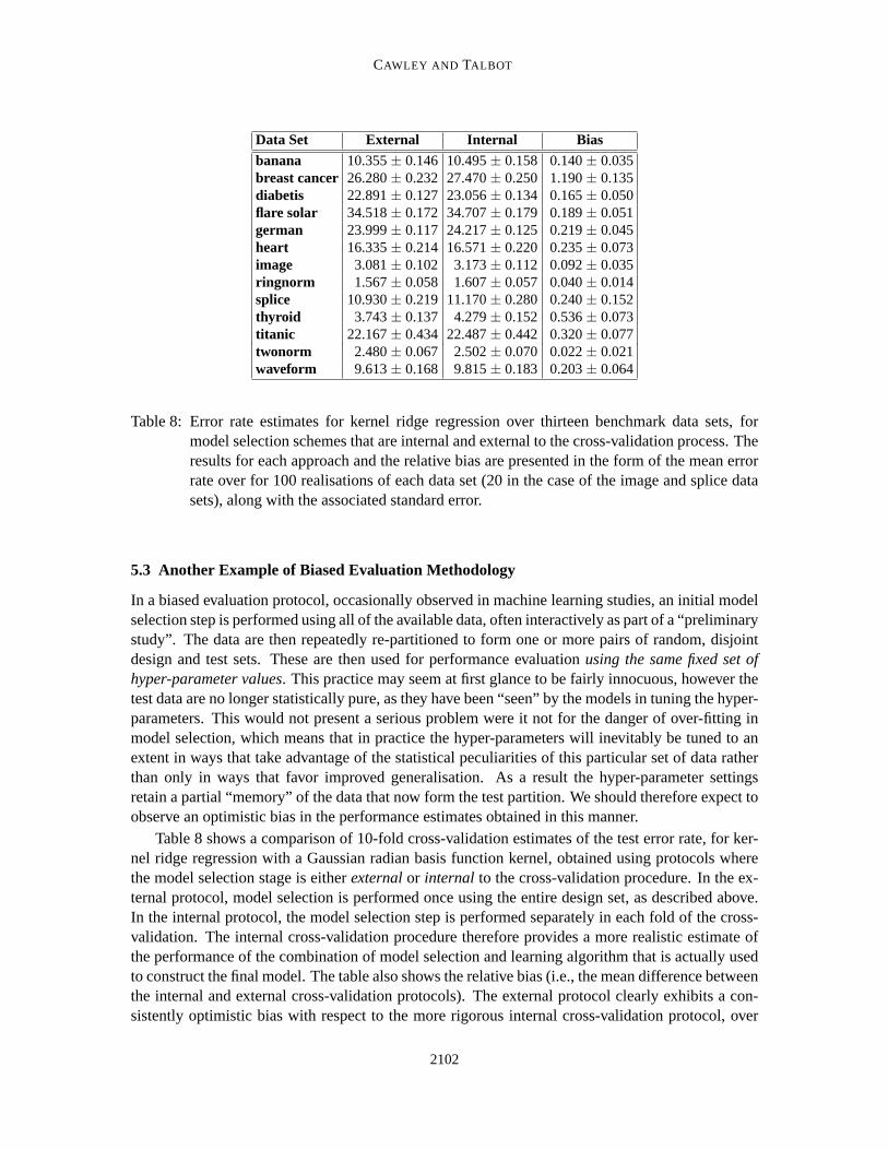
Table 8: Error rate estimates for kernel ridge regression over thirteen benchmark data sets, formodel selection schemes that are internal and external to the cross-validation process. Theresults for each approach and the relative bias are presented in the form of the mean errorrate over for 100 realisations of each data set (20 in the case of the image and splice datasets), along with the associated standard error.

5.3 Another Example of Biased Evaluation Methodology

In a biased evaluation protocol, occasionally observed in machine learningstudies, an initial modelselection step is performed using all of the available data, often interactivelyas part of a “preliminarystudy”. The data are then repeatedly re-partitioned to form one or more pairs of random, disjointdesign and test sets. These are then used for performance evaluationusing the same fixed set ofhyper-parameter values. This practice may seem at first glance to be fairly innocuous, however thetest data are no longer statistically pure, as they have been “seen” by the models in tuning the hyper-parameters. This would not present a serious problem were it not for the danger of over-fitting inmodel selection, which means that in practice the hyper-parameters will inevitably be tuned to anextent in ways that take advantage of the statistical peculiarities of this particular set of data ratherthan only in ways that favor improved generalisation. As a result the hyper-parameter settingsretain a partial “memory” of the data that now form the test partition. We shouldtherefore expect toobserve an optimistic bias in the performance estimates obtained in this manner.

Table 8 shows a comparison of 10-fold cross-validation estimates of the testerror rate, for ker-nel ridge regression with a Gaussian radian basis function kernel, obtained using protocols wherethe model selection stage is eitherexternalor internal to the cross-validation procedure. In the ex-ternal protocol, model selection is performed once using the entire design set, as described above.In the internal protocol, the model selection step is performed separately in each fold of the cross-validation. The internal cross-validation procedure therefore provides a more realistic estimate ofthe performance of the combination of model selection and learning algorithm that is actually usedto construct the final model. The table also shows the relative bias (i.e., the mean difference betweenthe internal and external cross-validation protocols). The external protocol clearly exhibits a con-sistently optimistic bias with respect to the more rigorous internal cross-validation protocol, over

2102


all thirteen benchmarks. Furthermore, the bias is statistically significant (i.e., larger than twice thestandard error of the estimate) for all benchmarks, apart fromsplice andtwonorm . In many cases,the bias is of similar magnitude to the typical difference observed between competitive learning al-gorithms (cf. Table 4). In some cases, for example,banana andthyroid benchmarks, the bias is ofa surprising magnitude, likely to be large enough to conceal even the true difference between evenstate-of-the-art and uncompetitive learning algorithms. This clearly showsthat the external cross-validation protocol exhibits a consistent optimistic bias, potentially of a very substantial magnitudeeven when the number of hyper-parameters is small (in this case only two), and so should not beused in practice.

6. Conclusions

In this paper, we have discussed the importance of bias and variance in model selection and perfor-mance evaluation, and demonstrated that a high variance can lead to over-fitting in model selection,and hence poor performance, even when the number of hyper-parameters is relatively small. Fur-thermore, we have shown that a potentially severe form of selection bias can be introduced intoperformance evaluation by protocols that have been adopted in a number of existing empirical stud-ies. Fortunately, it seems likely that over-fitting in model selection can be overcome using methodsthat have already been effective in preventing over-fitting during training, such as regularisation orearly stopping. Little attention has so far been focused on over-fitting in model selection, howeverin this paper we have shown that it presents a genuine pitfall in the practicalapplication of machinelearning algorithms and in empirical comparisons. In order to overcome the bias in performanceevaluation, model selection should be viewed as an integral part of the modelfitting procedure, andshould be conducted independently in each trial in order to prevent selection bias and because itreflects best practice in operational use. Rigorous performance evaluation therefore requires a sub-stantial investment of processor time in order to evaluate performance overa wide range of datasets, using multiple randomised partitionings of the available data, with model selection performedseparately in each trial. However, it is straightforward to fully automate thesesteps, and so requireslittle manual involvement. Performance evaluation according to these principlesrequires repeatedtraining of models using different sets of hyper-parameter values on different samples of the avail-able data, and so is also well-suited to parallel implementation. Given the recenttrend in processordesign towards multi-core designs, rather than faster processor speeds, rigorous performance eval-uation is likely to become less and less time-consuming, and so there is little justificationfor thecontinued use of potentially biased protocols.

Acknowledgments

The authors would like to thank Gareth Janacek, Wenjia Wang and the anonymous reviewers fortheir helpful comments on earlier drafts of this paper, and the organisers and participants of theWCCI-2006 Performance Prediction Challenge and workshop that provided the inspiration for ourwork on model selection and performance prediction. G. C. Cawley is supported by the Engineer-ing and Physical Sciences Research Council (EPSRC) grant EP/F010508/1 - Advancing MachineLearning Methodology for New Classes of Prediction Problems.

2103

CAWLEY AND TALBOT

References

D. M. Allen. The relationship between variable selection and prediction.Technometrics, 16:125–127, 1974.

C. Ambroise and G. J. McLachlan. Selection bias in gene extraction on the basis of microarray gene-expression data.Proceedings of the National Academy of Sciences, 99(10):6562–6566, May 142002. doi: 10.1073/pnas.102102699.

S. An, W. Liu, and S. Venkatesh. Fast cross-validation algorithms for least squares support vectormachines and kernel ridge regression.Pattern Recognition, 40(8):2154–2162, August 2007. doi:10.1016/j.patcog.2006.12.015.

E. Andelic, M. Schaffoner, M. Katz, S. E. Kruger, and A. Wendermuth. Kernel least-squares modelsusing updates of the pseudoinverse.Neural Computation, 18(12):2928–2935, December 2006.doi: 10.1162/neco.2006.18.12.2928.

Y. Bengio and Y. Grandvalet. No unbiased estimator of the variance of k-fold cross-validation.Journal of Machine Learning Research, 5:1089–1105, 2004.

S. A. Billings and K. L. Lee. Nonlinear Fisher discriminant analysis using a minimum squarederror cost function and the orthogonal least squares algorithm.Neural Networks, 15(2):263–270,March 2002. doi: 10.1016/S0893-6080(01)00142-3.

C. M. Bishop.Neural Networks for Pattern Recognition. Oxford University Press, 1995.

L. Bo, L. Wang, and L. Jiao. Feature scaling for kernel Fisher discriminant analysis using leave-one-out cross validation.Neural Computation, 18(4):961–978, April 2006. doi: 10.1162/neco.2006.18.4.961.

O. Bousquet and A. Elisseeff. Stability and generalization.Journal of Machine Learning Research,2:499–526, 2002.

L. Breiman. Random forests.Machine Learning, 45(1):5–32, October 2001. doi: 10.1023/A:1010933404324.

G. C. Cawley. Leave-one-out cross-validation based model selection criteria for weighted LS-SVMs. In Proceedings of the IEEE/INNS International Joint Conference on Neural Networks(IJCNN-06), pages 1661–1668, Vancouver, BC, Canada, July 16–21 2006. doi: 10.1109/IJCNN.2006.246634.

G. C. Cawley and N. L. C. Talbot. Efficient leave-one-out cross-validation of kernel Fisher dis-criminant classifiers.Pattern Recognition, 36(11):2585–2592, November 2003. doi: 10.1016/S0031-3203(03)00136-5.

G. C. Cawley and N. L. C. Talbot. Preventing over-fitting during model selection via Bayesianregularisation of the hyper-parameters.Journal of Machine Learning Research, 8:841–861, April2007.

2104


G. C. Cawley and N. L. C. Talbot. Efficient approximate leave-one-out cross-validation forkernel logistic regression.Machine Learning, 71(2–3):243–264, June 2008. doi: 10.1007/s10994-008-5055-9.

G. C. Cawley, G. J. Janacek, and N. L. C. Talbot. Generalised kernelmachines. InProceedings of theIEEE/INNS International Joint Conference on Neural Networks (IJCNN-07), pages 1720–1725,Orlando, Florida, USA, August 12–17 2007. doi: 10.1109/IJCNN.2007.4371217.

O. Chapelle, V. Vapnik, O. Bousquet, and S. Mukherjee. Choosing multipleparameters for sup-port vector machines.Machine Learning, 46(1–3):131–159, January 2002. doi: 10.1023/A:1012450327387.

H. Chen, P. Tino, and X. Yao. Probabilistic classification vector machines.IEEE Transactions onNeural Networks, 20(6):901–914, June 2009. doi: 10.1109/TNN.2009.2014161.

W. Chu, S. S. Keerthi, and C. J. Ong. Bayesian trigonometric support vector classifier. NeuralComputation, 15(9):2227–2254, September 2003. doi: 10.1162/089976603322297368.

J. Demsar. Statistical comparisons of classifiers over multiple data sets.Journal of Machine Learn-ing Research, 7:1–30, 2006.

R. O. Duda, P. E. Hart, and D. G. Stork.Pattern Classification. John Wiley and Sons, secondedition, 2001.

B. Efron and R. J. Tibshirani.Introduction to the Bootstrap. Monographs on Statistics and AppliedProbability. Chapman & Hall, 1994.

S. Geman, E. Bienenstock, and R. Doursat. Neural networks and the bias/variance dilemma.NeuralComputation, 4(1):1–58, January 1992. doi: 10.1162/neco.1992.4.1.1.

C. Gold, A. Holub, and P. Sollich. Bayesian approach to feature selectionand parameter tuningfor support vector machine classifiers.Neural Networks, 18(5):693–701, July/August 2005. doi:10.1016/j.neunet.2005.06.044.

I. Guyon, A. Saffari, G. Dror, and G. Cawley. Model selection: Beyond the Bayesian/frequentistdivide. Journal of Machine Learning Research, 11:61–87, 2009.

P. Hall and A. P. Robinson. Reducing the variability of crossvalidation forsmoothing parameterchoice.Biometrika, 96(1):175–186, March 2009. doi: doi:10.1093/biomet/asn068.

M. Kearns and D. Ron. Algorithmic stability and sanity-check bounds for leave-one-outcross-validation. Neural Computation, 11(6):1427–1453, August 1999. doi: 10.1162/089976699300016304.

G. S. Kimeldorf and G. Wahba. Some results on Tchebycheffian spline functions. Journal ofMathematical Analysis and Applications, 33:82–95, 1971.

S. R. Kulkarni, G. Lugosi, and S. S. Venkatesh. Learning pattern classification — a survey.IEEETransactions on Information Theory, 44(6):2178–2206, October 1998.

2105

CAWLEY AND TALBOT

P. A. Lachenbruch and M. R. Mickey. Estimation of error rates in discriminant analysis.Techno-metrics, 10(1):1–12, February 1968.

A. Luntz and V. Brailovsky. On estimation of characters obtained in statisticalprocedure of recog-nition (in Russian).Techicheskaya Kibernetica, 3, 1969.

D. J. C. MacKay. Bayesian interpolation.Neural Computation, 4(3):415–447, May 1992. doi:10.1162/neco.1992.4.3.415.

J. Mercer. Functions of positive and negative type and their connectionwith the theory of integralequations.Philosophical Transactions of the Royal Society of London, Series A, 209:415–446,1909.

S. Mika, G. Ratsch, J. Weston, B. Scholkopf, and K.-R. Muller. Fisher discriminant analysis withkernels. InNeural Networks for Signal Processing IX, Proceedings of the 1999 IEEE SignalProcessing Society Workshop, pages 41–48, Maddison, WI, USA, 21–25 August 1999. doi:10.1109/NNSP.1999.788121.

S. Mika, G. Ratsch, J. Weston, B. Scholkpf, and K.-R. Muller. Contructing descriptive and dis-criminative nonlinear features: Rayleigh coefficients in kernel feature spaces.IEEE Transactionson Pattern Analysis and Machine Intelligence, 25(5):623–628, May 2003. doi: 10.1109/TPAMI.2003.1195996.

J. A. Nelder and R. Mead. A simplex method for function minimization.Computer Journal, 7:308–313, 1965.

T. Pena Centeno and Lawrence N. D. Optimising kernel parameters and regularisation coefficientsfor non-linear discriminant analysis.Journal of Machine Learning Research, 7:455–491, Febru-ary 2006.

T. Poggio and F. Girosi. Networks for approximation and learning.Proceedings of the IEEE, 78(9):1481–1497, September 1990. doi: 10.1109/5.58326.

Y. Qi, T. P. Minka, R. W. Picard, and Z. Ghahramani. Predictive automatic relevance determinationby expectation propagation. InProceedings of the Twenty First International Conference onMachine Learning (ICML-04), pages 671–678, Banff, Alberta, Canada, July 4–8 2004.

C. E. Rasmussen and C. K. I. Williams.Gaussian Processes for Machine Learning. AdaptiveComputation and Machine Learning. MIT Press, 2006.

G. Ratsch, T. Onoda, and K.-R. Muller. Soft margins for AdaBoost.Machine Learning, 42(3):287–320, March 2001. doi: 10.1023/A:1007618119488.

R. M. Rifkin and R. A. Lippert. Notes on regularized least squares. Technical Report MIT-CSAIL-TR-2007-025, Computer Science and Artificial Intelligence Laboratory,MIT, May 2007.

B. D. Ripley. Pattern Recognition and Neural Networks. Cambridge University Press, 1996.

C. Saunders, A. Gammerman, and V. Vovk. Ridge regression learning algorithm in dual variables.In Proceedings of the Fifteenth International Conference on Machine Learning (ICML-98), pages515–521. Morgan Kaufmann, 1998.

2106


J. Shao. Linear model selection by cross-validation.Journal of the American Statistical Society,88:486–494, 1993.

I. Stewart. On the optimal parameter choice forν-support vector machines.IEEE Transactionson Pattern Analysis and Machine Intelligence, 25(10):1274–1284, October 2003. doi: 10.1109/TPAMI.2003.1233901.

M. Stone. Cross-validatory choice and assessment of statistical predictions. Journal of the RoyalStatistical Society, Series B (Statistical Methodology), 36(2):111–147, 1974.

M. Stone. Asymptotics for and against cross-validation.Biometrika, 64(1):29–35, April 1977. doi:10.1093/biomet/64.1.29.

J. A. K. Suykens, T. Van Gestel, J. De Brabanter, B. De Moor, and J.Vanderwalle.Least SquaresSupport Vector Machine. World Scientific Publishing Company, Singapore, 2002. ISBN 981-238-151-1.

A. N. Tikhonov and V. Y. Arsenin.Solutions of Ill-posed Problems. John Wiley, New York, 1977.

G. Toussaint. Bibliography on estimation of misclassification.IEEE Transactions on InformationTheory, IT-20(4):472–479, July 1974.

V. N. Vapnik. Estimation of Dependences Based on Empirical Data. Springer, 1982.

V. N. Vapnik. Statistical Learning Theory. Adaptive and learning systems for signal processing,communications and control series. Wiley, 1998.

S. Weisberg.Applied Linear Regression. Probability and Mathematical Statistics. John Wiley &Sons, second edition, 1985.

J. Weston. Leave-one-out support vector machines. InProceedings of the Sixteenth InternationalJoint Conference on Artificial Intelligence (IJCAI-99), pages 727–733, San Fransisco, CA, USA,1999. Morgan Kaufmann.

C. K. I. Williams and D. Barber. Bayesian classification with Gaussian processes. IEEE Trans-actions on Pattern Analysis and Machine Intelligence, 20(12):1342–1351, December 1998. doi:10.1109/34.735807.

P. M. Williams. A Marquardt algorithm for choosing the step size in backpropagation learning withconjugate gradients. Technical Report CSRP-229, University of Sussex, February 1991.

T. Zhang. Leave-one-out bounds for kernel machines.Neural Computation, 15(6):1397–1437, June2003. doi: 10.1162/089976603321780326.

2107

on over-fitting in model selection and subsequent selection bias in

Documents