1 (18)

Sample Selection Bias in the Swedish CPI

Kristina Strandberg and Anders Norberg, Statistics Sweden

e-mail: kristina.strandberg@scb.se, anders.norberg@scb.se

Paper presented at the Joint UNECE/ILO Meeting of the Group of Experts

on Consumer Price Indices, Geneva, Mya 26 – 28, 2014

0. Abstract

A bias occurs for a consumer price index, CPI, if price collectors avoid product

varieties on sale when selecting the sample in the reference month (December).

Once the sample is fixed, price collectors cannot avoid sales prices since they are

commissioned to collect prices almost as long as products are offered to

consumers for purchase. In December twelve months later the proportion of

reduced prices will normally be higher than in the reference month, creating a

downward bias in the CPI.

If price collectors favor products that have low campaign prices in the reference

month the opposite effect can occur.

Statistics Sweden (SCB) has applied an adjustment for selection bias for clothing

and footwear in the Swedish CPI and the HICP since 1993. It has been discussed

whether the same adjustment method is applicable and needed for other product

groups as well. In this report, we evaluate methods for hindering selection bias to

occur and explore the need for an adjustment of bias.

1. Sampling

The sampling of product offers has three stages; 1) sampling of outlets annually,

2) definitions of product groups (Strata) and definitions of the representative

items and finally, 3) the selection of specific product offers for the combinations

of outlets and representative items.

1.1 Sampling of Outlets

For product groups where local price collection or scanner data is used, outlets

are divided into 38 retail trade and service strata according to the Swedish

Standard Industrial Classification (SNI, which closely follows NACE, Rev. 2,

the EU standard). In each stratum a gross sample of units (outlets) is drawn from

the SAMU1 version of the Central Business Register by the method Sequential

Poisson sampling which is an order πps technique. This first gross sample is

drawn about six months before the year in which it is to be used. This sample is

screened in October and November, both in the central office and by the price

collectors visiting the units. Some of the units initially drawn are excluded for

various reasons. For example, they may be head offices rather than outlets, or

they may not sell any of the targeted products. After screening, outlets are picked

from the list one by one in order, until the predetermined net sample size is

1 SAMU is a tool used by a majority of the business surveys at Statistics Sweden to

establish a frame population to draw coordinated samples.

2 (18)

reached. Positive coordination of outlet samples between years is obtained

through the use of random numbers “permanently” associated with each outlet in

the sampling frame, Ohlsson (1995). Sampling rotation is performed so that 20

per cent of these random numbers are changed every year. Combined with

market changes, this results in some 70-75 per cent of outlets remaining in the

sample from one year (y-1) to the next (y).

1.2 Sampling of Representative Items

Following common practice, most products in the Swedish local price survey are

chosen using the representative item method. General product specifications are

drawn up in the central office using the Household Budget Survey (HBS) as one

reference among others. Price collectors then get specific instructions on how to

choose between the different varieties of each product.

Example 1 show four examples of product specifications from the central office.

Some products have tight specifications with several criterions for the price

collector to follow, illustrated here by the skirt. Other products, like yarn, have

more generic or loose specifications.

Example 1: Item specification and selected variety

Skirt: Size 38-42 or similar. Not a pantskirt. Not wool, linen or silk

Digital Camcorder: Digital recording, flash memory and HD supported

Skis: Cross country skis, suitable for a recreational skier, length 200 cm

Yarn: Wool, wool/synthetic mix or fully synthetic.

For daily necessities like food, beverages, detergents etc. SCB makes a probabi-

lity sample of fully specified products. Prices are collected from scanner data.

1.3 Sampling of Product Offers

Price collectors are instructed to choose the variety that is “most sold” in terms

of volume within the specification of the representative item. The ”most sold”

rule also applies to replacements when an item disappears from the market. This

method could be viewed as a special case of cutoff sampling. Outlet staff is often

asked to assist in the judgments that have to be made when applying this

criterion. For new varieties it is difficult to know in advance which items will

have the highest sale numbers. It is by no means certain that this selection

process in practice catches the variety that will be the most sold.

For the sample in the reference month, December year y, 25-30 per cent of the

product offers are new because the outlets are new in the sample. For the outlets

that are retained in the sample from the previous year, y-1, price collectors are

instructed to keep the same product offers as in the final sample of year y. New

product offers should be selected only if the old varieties no longer represent

consumer behavior, as is the instruction for any other month. By applying this

instruction the product offer is still the same for the final month of year y-1 as for

the reference month of year y.

1.4 Probability versus Non-Probability Sampling Techniques

Using judgmental sampling, i.e. letting price collectors choose the varieties when

creating the new sample in the reference period, is of course a non-probability

sampling technique. In a statistical setting, it is sometimes hard to argue the

benefits of such methods. International Labour Organization (2004) supports

such methods under certain circumstances (see Appendix A). In particular, when

3 (18)

non-probabilistic replacements are made throughout the measurement period the

benefits of a probability sample is destroyed (chapter 5.31).

There are draw backs of non-probability sampling. Since products are chosen

arbitrarily, there is no way to estimate the probability of any one product being

included in the sample. Also, no assurance is given that each item has a chance

of being included, making it impossible to estimate sampling variance. We

believe it is a fair assessment that judgment samples can be highly prone to

researcher bias. The selection bias introduced below, is a good example of how

the subjectivity of the price collector can create issues in the resulting sample.

2. The Problem

The Swedish CPI is a chain index with annual links. In December, prices are

collected for two partially overlapping samples from the same population:

1) the last measurement for year y-1 and 2) the first measurement for year y.

Every year about 25-30% of the outlets in the old sample are replaced and

thereby the same proportion of product offers are new. Instructions for price

collection say that all varieties, regardless of type of price, should be considered

when choosing the product offer. However, we have observed2 that price

collectors “prefer” products they expect to remain in stores longer to avoid

frequent replacements. When making the reference period selection, price

collectors therefore tend to choose varieties sold at regular price and not varieties

on sale, thereby creating a sample where sales prices are underrepresented.

While it is possible for the price collector to avoid varieties with sale prices in

the reference period, the proportion of sales prices in the December sample one

year later will reflect proportion of sale prices in the population more closely.

The relative lack of sales prices in the reference period will lead to a downward

bias in the CPI.

Norberg (1993) brought this problem to the attention of the CPI Advisory Board.

For the index year 1993 a correction/adjustment for the bias in clothing and

footwear was introduced, referred to as a “sales price correction3.” The actual

adjustment factors are not normally recorded and saved, but between 1994 and

1998 they were (Norberg, 1998):

2,17

2,43

2,40

3,68 and

1,14 percent

The adjustment factor for 1998 was low because the same sample of outlets was

used in 1997 and 1998. In can be noted that the estimated average bias for

clothing has been around two percentage points downwards annually, which

means a decrease in the total CPI of about 0.1 percentage points (Norberg, 1995

and 1998). Bias for footwear is somewhat lower.

2 The authors accompanied several price collectors to learn about the collection process.

We then made the observation that collectors purposely stay away from products with

sales prices when making replacements. 3 Since the introduction of the “sales price correction” it has become clear that the term is

unfortunate. It is not a correction for sales prices occurring during the year but rather for

the bias created when the price collector stays clear of sales prices when creating the base

sample. A better fitting term is therefore “adjustment for selection bias.”

4 (18)

An interesting aspect of the problem is that campaign prices can cause a bias in

the opposite direction of that caused by sales prices. The difference is found in

the character of the strategies behind the reduced prices. Sales are often used to

quickly sell out merchandise to make room for new products. Campaigns on the

other hand, can be used to introduce a new kind of merchandise or a seasonal

product. While product offers sold at a sale price can be expected to disappear

from the store, product offers part of a campaign are more likely to remain. The

price collectors act consequently and when sales prices are avoided, campaign

prices are inviting.

Figure 1 and 2 show the occurrence of sales and campaigns in prices for clothes,

shoes and other quality assessed products4 collected for the Swedish CPI

between January 2010 and March 2014. Of interest is how different the two price

strategies are; sales peak in January and July while campaigns seem to be more

common in December. It should be noted than the strong seasonal occurrence of

sale prices to a large extent is driven by the many price observations collected

from clothes and shoes. However, the same pattern is found for other products as

well, even if the effect is not as strong.

Figure 1: Frequency of sales prices in data for clothes, shoes and other quality assessed products, collected between January 2010 and March 2014.

Since the selection bias is caused by new products brought in to the sample in the

reference period of the new year (y) it is of interest to compare the frequency of

sales and campaigns for new products to the frequency of sales and campaigns of

old products in the reference sample. In figures 3 to 6 we see the frequencies of

sale or campaign prices in 2013 for products remaining in the sample from the

previous year. For a clearer view, Clothes and Shoes are separated from other

quality assessed products. Product group with no interesting sale or campaign

activities are left out of the plot. To illustrate the origin of the selection bias the

frequency of sales or campaigns for products introduced to the sample in the

reference period of 2013 are added to the plot.

4 Only products that are quality adjusted at price changes are included in the study since

those are the only products where regular prices are collected together with the sale price

continuously.

5 (18)

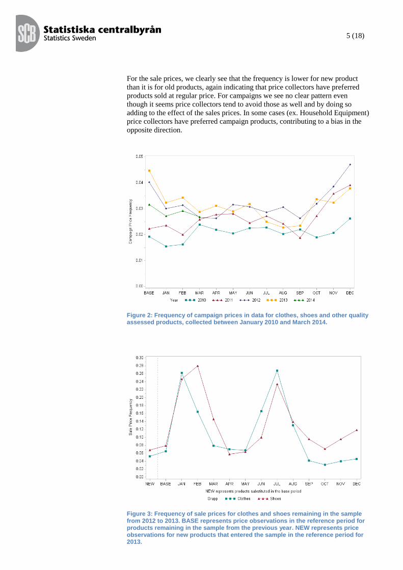
For the sale prices, we clearly see that the frequency is lower for new product

than it is for old products, again indicating that price collectors have preferred

products sold at regular price. For campaigns we see no clear pattern even

though it seems price collectors tend to avoid those as well and by doing so

adding to the effect of the sales prices. In some cases (ex. Household Equipment)

price collectors have preferred campaign products, contributing to a bias in the

opposite direction.

Figure 2: Frequency of campaign prices in data for clothes, shoes and other quality assessed products, collected between January 2010 and March 2014.

Figure 3: Frequency of sale prices for clothes and shoes remaining in the sample from 2012 to 2013. BASE represents price observations in the reference period for products remaining in the sample from the previous year. NEW represents price observations for new products that entered the sample in the reference period for 2013.

6 (18)

Figure 4: Frequency of campaign prices for clothes and shoes remaining in the sample from 2012 to 2013. BASE represents price observations in the reference period for products remaining in the sample from the previous year. NEW represents price observations for new products that entered the sample in the reference period for 2013.

Figure 5: Frequency of sale prices in 2013 for quality assessed products remaining in the sample from the previous year. BASE represents price observations in the reference period for products remaining in the sample from the previous year. NEW represents price observations for new products that entered the sample in the reference period for 2013.

To summarize, sale prices signals that the product offer will disappear from the

store. It is not favored by the price collector in the reference period since it will

cause a quick replacement. This will lead to a downward bias in the CPI. Product

7 (18)

offers sold in a campaign will remain in the store and they are very likely “most

sold.” Therefore they could be favored in the reference period and this could lead

to an upward bias in the CPI. However, it is obvious from Figure 2 that

campaigns are not as common as sales and we see no clear pattern of action from

the price collectors.

Figure 6: Frequency of campaign prices in 2013 for quality assessed products remaining in the sample from the previous year BASE represents price observations in the reference period for products remaining in the sample from the previous year. NEW represents price observations for new products that entered the sample in the reference period for 2013.

We suggest two groups of methods to deal with the selection bias;

Hinder the bias to arise

Adjust for the bias when/if it occurs

3. Methods for Avoiding the Bias

We present three methods for avoiding the bias that result when price collectors

tend to keep away from sales prices.

3.1 More Extensive Instructions to Price Collectors

Instructions say product variants sold at sale or campaign prices should be

selected if they are the most sold. Price itself must not be decisive for the

selection. Instructions are clear, but we can see a definite tendency that this

requirement is not fulfilled. We strongly question if more education of price

collectors would be a cost effective solution to the problem.

3.2 Draw New Samples in September or October

Selecting the sample for year y a couple of months earlier than the reference

period would allow the proportion of sales prices in the sample to increase until

they reach a stationary phase that is a good representation of the population. The

price measurements from the reference month (December) is then used for price

index calculations.

8 (18)

Norberg (1993) proposed that new samples were collected in November rather

than December for clothes. As it turned out, collecting the new sample one

month early did have some of the desired effect but it was not strong enough.

Although the selection bias was reduced, it was not completely eliminated. Up

for discussion is the possibility to draw the new sample already in September or

October. Three months might be enough for the proportion of sales prices in the

sample to better mimic that of the population.

One obvious drawback of carrying double samples is the added cost. For two or

three months price collectors will have to collect 25-30 per cent more prices ,

which will be more time consuming and expensive than collecting prices for one

sample.

On the other hand, an added benefit to drawing the new sample in September or

October would be the improvement in work environment for the price collectors.

Preparing a new sample and choosing new varieties in December, when

Christmas shopping is at a peak, is very stressful. It would be easier and less

stressful to perform this time consuming task in October when stores are not

heavily occupied by anxious Christmas shoppers.

3.3 Changing the CPI Linkage Months

December is not the best month to link short term indices based on the following

reasons:

There are a lot of price activities in December. Activities like end of

stock sales and campaigns brings variance to the price index link for the

month and chaining one index link with low statistical quality to another

with low statistical quality is worse than having two higher quality index

links. Table 1 below show the percentage of sale or campaign prices in

the sample, indicating that September and October are the overall best

choices for linking.

For working conditions for the price collectors in outlets it is an advan-

tage to move the almost double workload of the overlap period from

December to a less busy shopping month. September and October seems

to be good alternatives.

For working condition at the central CPI office at SCB it would be an

advantage to spread the heavy annual update workload over a longer

period.

A drawback with this method is that computation will be a little bit more

complex. The operationalization of the new index structure for the CPI as

suggested by Commission on the Review of the Swedish Consumer Price Index

(CPI), SOU 1999:124, documented in Ribe (2003), was approved by the CPI

Advisory Board at the meeting 219 in 2003.

The CPI construction works with a year-to-month-index my

gyI,

;2 for the product

group g , which in the simplest form is

my

gDy

Dy

gDy

m

my

gy

Dy

gDymy

gy II

I

II ,

;ec,1

ec,1

;ec,212

1

,2

;Dec,3

ec,2

;ec,3,

;2

12

1

.

9 (18)

For the months after September, if linking is indeed moved to September, the last

piece can be computed as

my

gSepty

Septy

gDy

my

gDy III ,

;,

,

;ec,1

,

;ec,1 .

In fact, the implementation can be made like imputation of reference prices. For

all product offers within a product group, the reference price for the last months

are the price in September divided by the index from December last year, y-

1,Dec to September current year, y,Sept.

Table 1: Percentage of price observations that are on sale or part of a campaign, per month 2010 to 2013.

Group

Month

1 2 3 4 5 6 7 8 9 10 11 12

Car Accessories 6 5 4 4 4 5 5 4 4 5 6 6

Clothes 31 21 12 10 9 18 32 19 7 7 9 12

Footwear 35 35 23 15 11 16 27 22 11 9 12 13

Furniture 9 7 6 6 6 7 8 6 5 6 6 6

High-Tech Products 16 10 11 13 12 14 19 11 10 13 10 9

Household Equipment 17 10 10 10 9 11 16 13 10 12 11 12

Household Goods 6 5 4 5 4 4 6 4 3 3 3 3

Household Textiles 20 16 14 15 10 16 17 18 12 14 14 17

Kitchen, Bath and Floors 6 7 7 7 6 7 6 6 5 9 9 8

Office Equipment 2 1 1 1 1 2 1 3 3 2 1 1

Optics 0 0 1 1 0 0 0 0 0 1 1 1

Other Personal Goods 14 14 13 16 15 15 16 17 14 9 10 12

Personal Hygiene 5 3 5 3 3 4 5 3 4 3 7 5

Tools & Garden Equipment 3 5 2 5 5 4 4 6 4 3 3 3

Toys and Sport Articles 16 19 20 16 15 16 18 16 16 16 15 15

Yarn & Fabric 1 2 1 1 0 0 1 1 1 0 0 0

4. Adjustment Method

December is the last month of last year’s link and the price reference period for

the next year’s link. This means that prices and information are collected for two

partially overlapping samples during the same week(s). Based on the two

samples we make two estimates of the effect of sales and campaigns on the mean

price level. If there is a purposive avoidance of sales prices in price reference

period, the effect of sale prices will be higher for the final December sample than

for the price reference period sample, for the identical period. The ratio between

these two estimates of the sales price effect is not only stochastic but also

systematic and would lead to a continuous bias in the CPI for the affected

products.

The formula for the index link for an elementary aggregate from December last

year y-1,Dec to the current month this year y,m in the Swedish CPI is

(∏

)

(∏

)

10 (18)

We use a similar formula as for the elementary aggregate of CPI-computation to

calculate the effect of sale prices. Put the observed prices in the place of the

comparison period prices, y,m, and the regular prices in the place of the price

reference period prices, y-1,12 to calculate the sales effects for the two samples.

For the final month of year y-1 we have for the product group g

(∏

)

(∏

)

For the reference month of year y we have

(∏

)

(∏

)

The bias of the prices of the base period is on average

Prices in the reference month are now adjusted by the ratio of the sales price

effect for the final December sample and the sales price effect for the price

reference period sample (1/BIAS). Alternatively an adjustment to the monthly

price index is made by the ratio between the sales price effect of the reference

month of the new sample to that of the final month of the old sample (BIAS).

This adjustment is applied during the following year, y.

Example 2: Calculation of Adjustment for Selection Bias All prices are collected in December some year y-1. There are four varieties

in the survey of the present year y-1 and five varieties to be measured the

following year y beginning in this month December.

Final month of last year's link Price ref. month of new year link

Regular price

Actual

price Regular price

Actual

price

199 199 199 199

199 149 199 149

98 98 98 98

595 495

599 599

899 899

Index (actual/regular)

= 88.8

Index (actual/regular)

= 94.4

In this example two out of four varieties had sales prices in the final month of

last year’s link and the actual prices were on average 88.8 per cent of the regular

prices. Analogously the actual prices in the new price reference period sample

were on average 94.4 per cent of the regular prices. The price index for every

month of the new year must be adjusted up-wards with the ratio 94.4/88.8 =

1.062.

11 (18)

5. Analysis of CPI Data

5.1 Data

Analysis has been carried out on real CPI data from the years 2010, 2011, 2012

and 2013 to see if any product and industry combination shows a big selection

bias, indicating that some kind of action, either to prevent the bias from

occurring or adjust for it when it occurs, would be beneficial.

Tableau: Product categories considered in this study

Category Products

Clothing All clothing

Footwear All footwear

High-tech products Television set, CD/cassette player, stereo, camcorder, DVD player, home theatre, MP3 player

Household goods China and utensils, drinking glass, pots and pans, kitchen scales

Household textiles Towel, bedding, comforter, curtains and cloth for curtains

Recreational goods Toys, sport articles, ski equipment, recreational goods, bike, music instruments

Personal hygiene Cosmetics, electric razor

Furniture Kitchen table, chair, upholstered chair, sofa, mirror, bed, shelves, rug, mattress, ceiling lamp

Car accessories Tires, car accessories, booster seat

Optics Glasses, contact lenses

Household equipment Laundry machine, dishwashing machine, vacuum cleaner, electric stove, refrigerator, microwave oven, coffee maker, water boiler

Yarn and fabric Yarn, thread, fabric

Kitchen, bath and interior Bathtub, toilet, kitchen cupboard, kitchen sink, wooden floor, door

Tools and garden equipment Hammer, grass mower, knife, garden spade, light bulb, electric screwdriver

Office equipment Writing paper, ink for printer

Other personal goods Watch, bag

5.2 Results

Results from the analysis can be seen in the tables 2-5 (tables 4 and 5 are found

in Appendix B.

It is not uncommon that some products have low counts in some of the industries

and thereby accidently introduce a significant bias. For example, in 2011 the bias

for baby pants sold in hypermarkets is extremely high (Table 5 in appendix B). A

closer inspection of the prices show that there are eight pairs of baby pants sold

in hypermarkets in the reference period with only one pair sold at a discount. In

December twelve months later there is only one pair left, sold at 35% of the

original price.

Clothing and footwear are adjusted for the selection bias every year. Looking at

table 2 it is clear that this adjustment is motivated. The extent of the bias varies

from year to year and depends on the particular product varieties chosen in the

reference month sample.

12 (18)

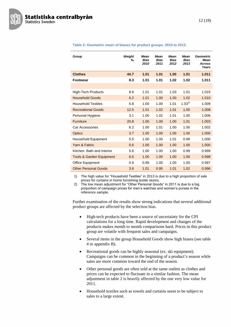
Table 2: Geometric mean of biases for product groups. 2010 to 2013.

Group

Weight

‰

Mean Bias 2010

Mean Bias 2011

Mean Bias 2012

Mean Bias 2013

Geometric

Mean Across

Years

Clothes 44.7 1.01 1.01 1.00 1.01 1.011

Footwear 8.3 1.01 1.01 1.02 1.02 1.011

High-Tech Products 8.6 1.01 1.01 1.03 1.01 1.015

Household Goods 6.2 1.01 1.00 1.00 1.02 1.010

Household Textiles 5.8 1.00 1.00 1.01 1.031)

1.009

Recreational Goods 12.5 1.01 1.02 1.01 1.00 1.008

Personal Hygiene 3.1 1.00 1.02 1.01 1.00 1.006

Furniture 20.8 1.00 1.00 1.00 1.01 1.003

Car Accessories 6.2 1.00 1.01 1.00 1.00 1.002

Optics 3.7 1.00 1.00 1.00 1.00 1.000

Household Equipment 5.5 1.00 1.00 1.01 0.99 1.000

Yarn & Fabric 0.6 1.00 1.00 1.00 1.00 1.000

Kitchen. Bath and Interior 5.6 1.00 1.00 1.00 0.99 0.999

Tools & Garden Equipment 6.5 1.00 1.00 1.00 1.00 0.998

Office Equipment 0.9 0.99 1.00 1.00 1.00 0.997

Other Personal Goods 3.6 1.01 0.95

1.01 1.02 0.996

1) The high value for “Household Textiles” in 2013 is due to a high proportion of sale prices for curtains in home furnishing textile stores.

2) The low mean adjustment for “Other Personal Goods” in 2011 is due to a big proportion of campaign prices for men’s watches and women’s purses in the reference sample.

Further examination of the results show strong indications that several additional

product groups are affected by the selection bias.

High-tech products have been a source of uncertainty for the CPI

calculations for a long time. Rapid development and changes of the

products makes month to month comparisons hard. Prices in this product

group are volatile with frequent sales and campaigns.

Several items in the group Household Goods show high biases (see table

4 in appendix B).

Recreational goods can be highly seasonal (ex. ski equipment).

Campaigns can be common in the beginning of a product’s season while

sales are more common toward the end of the season.

Other personal goods are often sold at the same outlets as clothes and

prices can be expected to fluctuate in a similar fashion. The mean

adjustment in table 2 is heavily affected by the one very low value for

2011.

Household textiles such as towels and curtains seem to be subject to

sales to a large extent.

13 (18)

5.3 Discussion of Method

During the measurement year the products chosen in the original sample will go

on sale and finally disappear and get replaced. In this fashion, the sample will

evolve from the originally low proportion of sales prices toward a proportion of

sales prices close to that of the general population. If price collectors in

December chose products completely new to the market we can expect this

process to take several months since sales prices usually occur in the tail end of

the product life. Since the adjustment factor is the same for all month of the

measurement year we could end up with a reverse bias in the beginning of the

year. Even if this is the case, the adjustment of selection bias will have a positive

effect overall.

Another thing to keep in mind is the quality of the reported regular prices.

Calculations of the bias is dependent on the assumption that the regular price of a

sale item is “correct”. For some product groups it is common practice to use

“recommended price” or “list price” rather than a “true” regular price. A

recommended price is almost never paid by the customer, but is used to make a

sale price more attractive. In such cases we would overestimate the selection

bias.

If all observed regular prices are generally X % higher than the “true” regular

prices there will be no effect on the adjustment for the selection bias. If, on the

other hand, regular prices for sale products are increased to make the sale appear

better, we will overestimate the selection bias. Table 3 shows that this practice is

not very common in Sweden. It appears that it is as common for the regular price

to decrease before a sale.

Table 3: Change of regular price from month before the sale price to the month with sale price. Proportions of price observations with price decrease and price increase.

Group

Decrease (%)

Increase (%)

Number

of obs

Car Accessories 1.7 2.3 346

Clothes 1.1 0.5 12 591

Footwear 1.0 0.9 5 078

Furniture 1.5 1.8 1 499

High-Tech Products 3.4 2.5 1 551

Household Equipment 2.9 3.0 1 811

Household Goods 1.2 1.6 429

Household Textiles 2.3 3.0 1 898

Kitchen. Bath & Floors 1.1 1.8 438

Office Equipment 7.5 5.7 53

Optics 0.0 0.0 10

Other Personal Goods 0.7 1.7 539

Personal Hygiene 1.7 2.2 179

Tools & Garden Equipment 1.5 2.3 263

Recreational Goods 0.9 2.0 2 056

Yarn & Fabric 10.0 0.0 10

14 (18)

We realize that the quality or relevance of regular prices can be questioned. After

examination of the regular prices in the Swedish CPI system, our opinion is that

they are trustworthy and of good enough quality to use in our bias calculations.

It should also be mentioned that since the estimates of the effects of sales prices

are stochastic, big (or small) values of the bias adjustment can appear randomly.

Table 5 in Appendix B shows that in 2011, the adjustment for baby pants in

hypermarkets is 2.48 which must be considered uncommonly high. In this case

there was only one product offer. It is obvious that the estimated bias has high

variance but there is also a strong negative covariance between the estimated

adjustment factor for year y and the index link between December year y-2 and

December year y-1. Adjusting for the bias should therefore result in less variance

in estimates of long term price movement.

6. Conclusions

Statistics Sweden has adjusted for the selection bias for clothing and footwear for

the past 20 years. Analysis carried out in this study supports this and continues to

point out clothing and footwear as product groups where selection bias is

present. Other product groups where the analysis indicate there is a selection bias

are High-Tech products, Household Goods, Household Textiles, Recreational

Goods and Other Personal Goods. The bias is not as strong or consistent in these

product groups, but sometimes big enough that something should be done to

counteract it.

Applying the method of adjusting for the selection bias to all or some of the

above mentioned product groups seems an intuitive solution to the problem. For

more uncommon situations as the example with a reverse bias due to campaign

prices in the reference month (i.e. the proportion of reduced prices is higher in

the reference sample than in the population) an adjustment will also be

beneficial.

Criticism of the correction method is that it appears to be volatile. As the

analysis show, some products can sometimes show “accidently” high biases due

to low counts in some products. This is variance. The quality of the “regular

prices” is also a matter of concern, the objection is that the so called regular

prices are not relevant or “true”.

After careful consideration and discussion in the Swedish CPI Advisory Board

the method we recommend for dealing with the selection bias is early selection

of the new sample. By choosing the new sample already in September or

October, the proportion of sale or campaign prices will mimic those in the

population. Although more expensive, this method is preferable over the

adjustment method since it is better to hinder the bias to arise than to adjust for it

when it is reality. For clothing and footwear the present adjustment method is

approved.

7. References

International Labour Organization (2004): The Consumer Price Index Manual:

Theory and Practice

Norberg, A. (1993-07-27): Förslag till reviderad metod för beräkning av

prisutvecklingen för kläder i konsumentprisindex, Paper presented at the

Swedish CPI Advisory Board, meeting 183, 1993.

15 (18)

Norberg, A. (1995-10-24): Quality Adjustment in the Swedish Price Index for

Clothing. Paper prepared for the Second Meeting of the International Working

Group on Price Indices, Stockholm 15-17 November, 1995.

Norberg, A. (1998-09-16): Behandling av kvalitetsförändringar på varor och

tjänster i KPI december 1997 – juli 1998. Paper presented at the Swedish CPI

Advisory Board, meeting 199. 1998.

Norberg, A. (1998-10-13): Quality Adjustment of Clothing in the Swedish

Consumer Price Index. Paper prepared for the statistical conference

“Methodological Issues in Official Statistics”, Stockholm 12 – 13 October 1998.

Ohlsson, E. (1990), Sequential Poisson Sampling from a Business Register and

its Application to the Swedish Consumer Price Index,

R&D Report 1990:6

Ohlsson, E. (1995): Coordination of Samples Using Permanent Random

Numbers. In Cox et al.: Business Survey Methods, Wiley, pp. 153-169

Ribe, M. (2003-05-26): Operationalisering av ny indexkonstruktion för KPI efter

KPI-utredningen. Promemoria presented at the Swedish CPI Advisory Board,

meeting 219, 2003.

16 (18)

Appendix A: The Consumer Price Index Manual

Reasons for using non-probability sampling 5.28 No sampling frame is available. This is often

true for the product dimension but less frequently so for

the outlet dimension, for which business registers or

telephone directories do provide frames, at least in some

countries, notably in Western Europe, North America

and Oceania. There is also the possibility of constructing

tailor-made frames in a limited number of cities or locations,

which are sampled as clusters in a first stage. For

products, it may be noted that the product assortment

exhibited in an outlet provides a natural sampling

frame, once the outlet is sampled as a kind of cluster, as

in the BLS sampling procedure presented above. So the

absence of sampling frames is not a good enough excuse

for not applying probability sampling.

5.29 Bias resulting from non-probability sampling is

negligible. There is some empirical evidence to support

this assertion for highly aggregated indexes. Dalén

(1998b) and De Haan, Opperdoes and Schut (1999)

both simulated cut-off sampling of products within item

groups. Dalén looked at about 100 groups of items sold

in supermarkets and noted large biases for the sub-indices

of many item groups, which however almost

cancelled out after aggregation. De Haan, Opperdoes

and Schut used scanner data and looked at three categories

(coffee, babies’ napkins and toilet paper) and,

although the bias for any one of these was large, the

mean square error (defined as the variance plus the

squared bias) was often smaller than that for pps

sampling. Biases were in both directions and so could

be interpreted to support Dale´ n’s findings. The large

biases for item groups could, however, still be disturbing.

Both Dalén and De Haan, Opperdoes and Schut

report biases for single-item groups of many index

points.

5.30 We need to ensure that samples can be monitored

for some time. If we are unlucky with our probability

sample, we may end up with a product that disappears

immediately after its inclusion in the sample. We are then

faced with a replacement problem, with its own bias

risks. Against this, it may happen that short-lived products

have a different price movement from the price

movement of long-lived ones and constitute a significant

part of the market, so leaving them out will create bias.

5.31 A probability sample with respect to the base

period is not a proper probability sample with respect to

the current period. This argument anticipates some of the

discussion in Chapter 8 below. It is certainly true that

the bias protection offered by probability sampling is to

a large extent destroyed by the need for non-probabilistic

replacements later on.

17 (18)

Appendix B: Result Tables

Table 4: Products and industries with the largest biases in 2013.

Product

Industry

Index Dec

n Dec

Index Base

n Base

BIAS

Drinking glass Glassware. china and kitchenware

90.24 7 100.00 12 1.11

Salad bowl Glassware. china and kitchenware

88.46 8 97.42 11 1.10

Floor mat Home furnishing textiles 64.32 3 70.73 2 1.10

Woman's coat Clothing 79.89 58 87.59 71 1.10

Street shoe Hypermarkets 93.87 7 100.00 6 1.07

Digital camera Photographic equipment 89.00 12 94.72 15 1.06

Cordless telephone Telecommunications equipment

90.34 37 95.29 37 1.05

Curtain Home furnishing textiles 82.37 40 86.40 43 1.05

Men's watch Watches and clocks 84.42 18 88.07 24 1.04

Men's shoe Footwear 90.68 39 94.54 40 1.04

Woman's wool coat Clothing 87.14 78 90.71 122 1.04

Curtain Hypermarkets 92.50 19 96.26 18 1.04

Floor hockey stick Sport and leisure 84.96 77 88.07 87 1.04

Rubber boots Sport and leisure 94.88 23 98.12 27 1.03

Gloves Sport and leisure 91.39 28 94.44 33 1.03

Coffee mug Hypermarkets 95.31 23 98.38 25 1.03

Suite case Hypermarkets 91.86 21 94.64 20 1.03

Men's sweater Clothing 93.37 107 96.10 126 1.03

Wall mounted mirror Home furniture 97.46 27 100.00 24 1.03

Woman's boots Footwear 91.30 68 93.60 66 1.03

Woman's heavy boots Footwear 93.60 92 95.79 89 1.02

Men's heavy boot Footwear 94.78 104 96.94 102 1.02

Woman's skirt Clothing 92.05 82 94.14 119 1.02

Woman's pumps Footwear 90.99 82 93.03 91 1.02

Salad bowl Hypermarkets 90.60 7 92.61 9 1.02

… …

Booster seat Other retail sale in specialized stores n.e.c.

91.31 14 89.94 12 0.98

Stroller Other retail sale in specialized stores n.e.c.

96.26 23 94.72 21 0.98

Door. storage unit Wood and other building material

100.00 18 98.17 19 0.98

Mountain bike Sport and leisure 94.38 36 92.59 37 0.98

Washing machine Electrical household appliances

91.96 13 90.15 20 0.98

Jeans Sport and leisure 92.18 5 90.32 4 0.98

Men's coat Sport and leisure 91.24 67 89.37 79 0.98

Espresso machine Hypermarkets 89.72 18 87.77 18 0.98

Pot Hypermarkets 99.21 12 97.01 16 0.98

Pot Glassware. china and kitchenware

96.86 7 94.61 10 0.98

Electric razor Electrical household appliances

100.00 8 97.14 11 0.97

Hammer Hypermarkets 100.00 11 96.30 13 0.96

Cordless screw driver Wood and other building material

100.00 16 95.78 20 0.96

Coffee maker Electrical household appliances

99.32 14 94.88 18 0.96

Refrigerator Electrical household appliances

96.49 7 92.11 10 0.95

Mountain bike Hypermarkets 81.64 10 77.60 11 0.95

18 (18)

Table 5: Products and industries with the largest biases in 2011.

Product

Industry

Index Dec

n Dec

Index Base

n Base

BIAS

Baby pant Hypermarkets 35,35 1 87,81 8 2,48

Man's shirt Hypermarkets 49,75 1 100,00 5 2,01

Home theatre Photographic equipment, specialized stores

62,50 1 88,23 1 1,41

Floor mat Hypermarkets 78,52 3 100,00 5 1,27

Television set, small Photographic equipment, specialized stores

79,99 1 100,00 2 1,25

Men's coat Hypermarkets 84,09 4 100,00 5 1,19

Jeans Hypermarkets 83,31 8 96,84 9 1,16

Electric razor Electrical household appliances, specialized stores

86,37 8 100,00 8 1,16

Dishwashing machine Electrical fittings, specialized stores

83,26 1 91,25 2 1,10

Woman's coat Sport and leisure goods 88,30 10 96,48 46 1,09

Digital camcorder Photographic equipment, specialized stores

86,30 3 93,88 7 1,09

Children’s sweater Hypermarkets 92,15 17 100,00 11 1,09

Floor hockey stick Sport and leisure goods 86,00 36 91,59 60 1,06

Electric razor Electrical fittings, specialized stores

88,52 2 94,09 4 1,06

Wool coat Clothing 86,55 45 91,77 46 1,06

Storage unit doors Wood and other building material

92,43 21 97,94 10 1,06

Dishwashing machine Electrical household appliances, specialized stores

92,58 8 97,25 8 1,05

Woman's wool coat Clothing 84,07 106 88,11 88 1,05

Television set, big Photographic equipment, specialized stores

95,74 2 100,00 4 1,04

Towel Home furnishing textiles, specialized stores

72,12 30 75,30 37 1,04

Men's pullover Sport and leisure goods 92,36 13 96,40 19 1,04

Women's top Sport and leisure goods 94,62 19 98,65 46 1,04

Digital camera Hypermarkets 89,60 5 93,36 8 1,04

Electric kettle Electrical fittings, specialized stores

90,86 4 94,67 7 1,04

Towel Hypermarkets 94,39 31 98,10 36 1,04

Back pack Sport and leisure goods 91,76 12 95,36 17 1,04

Toilet Carpets, rugs, wall and floor coverings, specialized stores

89,42 2 92,82 3 1,04

Push chair for kids Games and toys, specialized stores

95,91 30 99,50 25 1,04

Beddings Home furniture, specialized stores

93,46 41 96,90 44 1,04

Women's dress Clothing 93,82 78 97,24 95 1,04