on incidence between strata of the hilbert scheme of points on
TRANSCRIPT

Math. Z. (2007) 255:897–922DOI 10.1007/s00209-006-0057-4 Mathematische Zeitschrift
On incidence between strata of the Hilbert schemeof points on P
2
Koen De Naeghel · Michel Van den Bergh
Received: 17 March 2005 / Accepted: 31 July 2006 /Published online: 15 November 2006© Springer-Verlag 2006
Abstract The Hilbert scheme of n points in the projective plane has a naturalstratification obtained from the associated Hilbert series. In general, the precise inclu-sion relation between the closures of the strata is still unknown. Guerimand, Ph.DThesis, Universite’de Nice, 2002 studied this problem for strata whose Hilbert seriesare as close as possible. Preimposing a certain technical condition he obtained neces-sary and sufficient conditions for the incidence of such strata. In this paper we presenta new approach, based on deformation theory, to Guerimand’s result. This allows usto show that the technical condition is not necessary.
Keywords Projective plane · Hilbert scheme of points · Incidence · Stratification ·Deformation
Mathematics Subject Classification (1991) Primary 14C99
1 Introduction and main result
Below k is an algebraically closed field of arbitrary characteristic and A = k[x, y, z].We will consider the Hilbert scheme Hilbn(P
2) parametrizing zero-dimensionalsubschemes of length n in P
2. It is well known that this is a smooth connected projectivevariety of dimension 2n.
Michel Van den Bergh is a director of research at the FWO.
K. De Naeghel (B) · M. Van den BerghDepartement WNI, Limburgs Universitair Centrum, Universitaire Campus, Building D,3590 Diepenbeek, Belgiume-mail: [email protected]; [email protected]
M. Van den Berghe-mail: [email protected]
898 K. De Naeghel, M. Van den Bergh
Associated to X ∈ Hilbn(P2) there is an ideal IX ⊂ O
P2 and a graded ideal IX =
⊕nH0(P2, IX(n)) ⊂ A. The Hilbert function hX of X is the Hilbert function of thegraded ring A(X) = A/IX . Classically hX(m) is the number of conditions for a curveof degree m to contain X. Clearly hX(m) = n for m � 0.
It seems Castelnuovo was the first to recognize the utility of the difference function(see [5])
sX(m) = hX(m)− hX(m − 1)
Thus sX(m) = 0 for m � 0. Knowing sX we can reconstruct hX .It is known [5,8,11] that a function h is of the form hX for X ∈ Hilbn(P
2) if andonly if h(m) = 0 for m < 0 and h(m)− h(m − 1) is a so-called Castelnuovo function ofweight n.
A Castelnuovo function [5] by definition has the form
s(0) = 1, s(1) = 2, . . . , s(σ − 1) = σ and s(σ − 1) ≥ s(σ ) ≥ s(σ + 1) ≥ · · · ≥ 0.(1.1)
for some integer σ ≥ 0, and the weight of s is the sum of its values.It is convenient to visualize s using the graph of the staircase function
Fs : R → N : x �→ s(x)
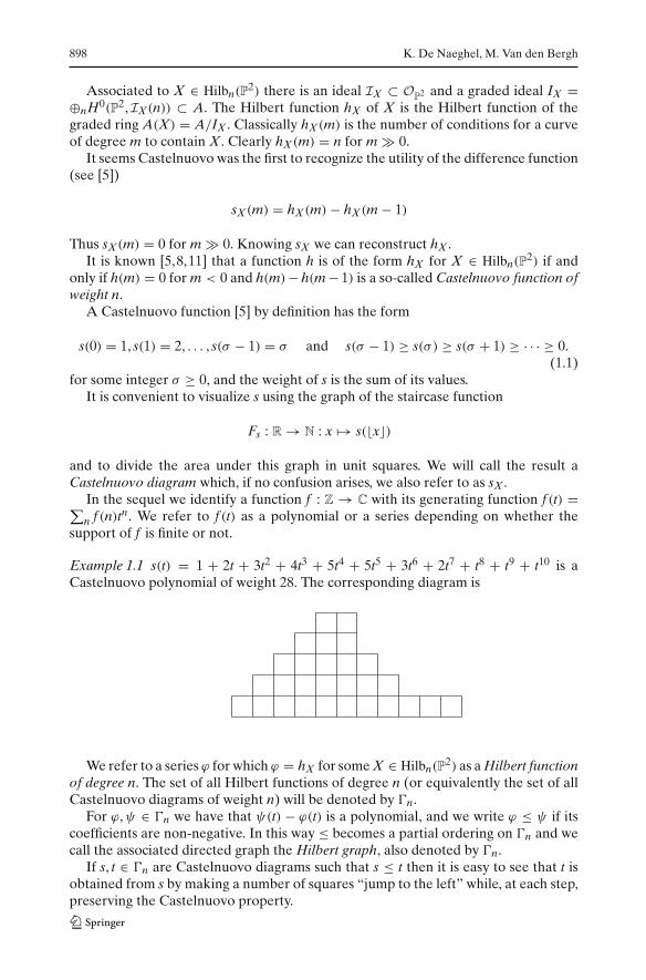
and to divide the area under this graph in unit squares. We will call the result aCastelnuovo diagram which, if no confusion arises, we also refer to as sX .
In the sequel we identify a function f : Z → C with its generating function f (t) =∑n f (n)tn. We refer to f (t) as a polynomial or a series depending on whether the
support of f is finite or not.
Example 1.1 s(t) = 1 + 2t + 3t2 + 4t3 + 5t4 + 5t5 + 3t6 + 2t7 + t8 + t9 + t10 is aCastelnuovo polynomial of weight 28. The corresponding diagram is
We refer to a series ϕ for which ϕ = hX for some X ∈ Hilbn(P2) as a Hilbert function
of degree n. The set of all Hilbert functions of degree n (or equivalently the set of allCastelnuovo diagrams of weight n) will be denoted by �n.
For ϕ,ψ ∈ �n we have that ψ(t) − ϕ(t) is a polynomial, and we write ϕ ≤ ψ if itscoefficients are non-negative. In this way ≤ becomes a partial ordering on �n and wecall the associated directed graph the Hilbert graph, also denoted by �n.
If s, t ∈ �n are Castelnuovo diagrams such that s ≤ t then it is easy to see that t isobtained from s by making a number of squares “jump to the left” while, at each step,preserving the Castelnuovo property.

On incidence between strata of the Hilbert scheme of points on P2 899
Example 1.2 There are two Castelnuovo diagrams of weight 3.
≤
These distinguish whether three points are collinear or not. The correspondingHilbert functions are 1, 2, 3, 3, 3, 3, . . . and 1, 3, 3, 3, 3, 3, . . ..
Remark 1.3 The number of Castelnuovo diagrams with weight n is equal to the num-ber of partitions of n with distinct parts (or equivalently the number of partitions of nwith odd parts) [7]. In loc. cit. there is a table of Castelnuovo diagrams of weight upto 6 as well as some associated data. The Hilbert graph is rather trivial for low valuesof n. The case n = 17 is more typical (see Appendix A).
Hilbert functions provide a natural stratification of the Hilbert scheme. For anyHilbert function ψ of degree n one defines a smooth connected subscheme [7,10] Hψ
of Hilbn(P2) by
Hψ = {X ∈ Hilbn(P2) | hX = ψ}.
The family {Hψ }ψ∈�n forms a stratification of Hilbn(P2) in the sense that
Hψ ⊂⋃
ϕ≤ψHϕ
It follows that if Hϕ ⊂ Hψ then ϕ ≤ ψ . The converse implication is in general falseand it is still an open problem to find necessary and sufficient conditions for the exis-tence of an inclusion Hϕ ⊂ Hψ [2–4,14]. This problem is sometimes referred to as theincidence problem.
Guerimand in his PhD-thesis [12] introduced two additional necessary conditionsfor incidence of strata which we now discuss.
the dimension condition: dim Hϕ < dim Hψ (1.2)
This criterion can be used effectively since there are formulas for dim Hψ [7,10].The tangent function tϕ of a Hilbert function ϕ ∈ �n is defined as the Hilbert
function of IX ⊗P
2 TP
2 , where X ∈ Hϕ is generic. Semi-continuity yields:
the tangent condition: tϕ ≥ tψ (1.3)
Again it is possible to compute tψ fromψ (see [12, Lemme 2.2.4] and also Proposition3.3.1 below).
Let us say that a pair of Hilbert functions (ϕ,ψ) of degree n has length zero ifϕ < ψ and there are no Hilbert functions τ of degree n such that ϕ < τ < ψ .1 It iseasy to see (ϕ,ψ) has length zero if and only if the Castelnuovo diagram of ψ can beobtained from that of ϕ by making a minimal movement to the left of one square [12,Proposition 2.1.7].
1 This is a minor deviation from Guerimand’s definition.
900 K. De Naeghel, M. Van den Bergh
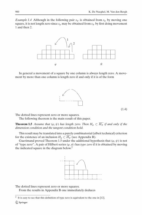
Example 1.4 Although in the following pair sψ is obtained from sϕ by moving onesquare, it is not length zero since sϕ may be obtained from sψ by first doing movement1 and then 2.
ϕ ψ
12
In general a movement of a square by one column is always length zero. A move-ment by more than one column is length zero if and only if it is of the form
(1.4)
The dotted lines represent zero or more squares.The following theorem is the main result of this paper.
Theorem 1.5 Assume that (ϕ,ψ) has length zero. Then Hϕ ⊂ Hψ if and only if thedimension condition and the tangent condition hold.
This result may be translated into a purely combinatorial (albeit technical) criterionfor the existence of an inclusion Hϕ ⊂ Hψ (see Appendix B).
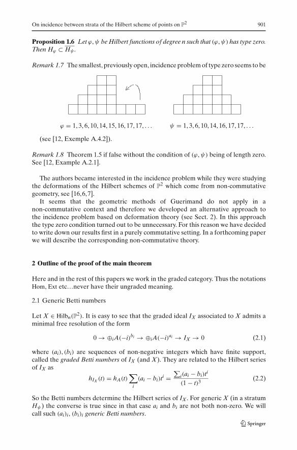
Guerimand proved Theorem 1.5 under the additional hypothesis that (ϕ,ψ) is notof “type zero”. A pair of Hilbert series (ϕ,ψ) has type zero if it is obtained by movingthe indicated square in the diagram below.2
The dotted lines represent zero or more squares.From the results in Appendix B one immediately deduces
2 It is easy to see that this definition of type zero is equivalent to the one in [12].
On incidence between strata of the Hilbert scheme of points on P2 901
Proposition 1.6 Let ϕ,ψ be Hilbert functions of degree n such that (ϕ,ψ) has type zero.Then Hϕ ⊂ Hψ .
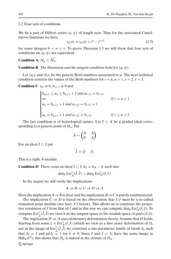
Remark 1.7 The smallest, previously open, incidence problem of type zero seems to be
ϕ = 1, 3, 6, 10, 14, 15, 16, 17, 17, . . . ψ = 1, 3, 6, 10, 14, 16, 17, 17, . . .
(see [12, Exemple A.4.2]).
Remark 1.8 Theorem 1.5 if false without the condition of (ϕ,ψ) being of length zero.See [12, Example A.2.1].
The authors became interested in the incidence problem while they were studyingthe deformations of the Hilbert schemes of P
2 which come from non-commutativegeometry, see [16,6,7].
It seems that the geometric methods of Guerimand do not apply in anon-commutative context and therefore we developed an alternative approach tothe incidence problem based on deformation theory (see Sect. 2). In this approachthe type zero condition turned out to be unnecessary. For this reason we have decidedto write down our results first in a purely commutative setting. In a forthcoming paperwe will describe the corresponding non-commutative theory.
2 Outline of the proof of the main theorem
Here and in the rest of this papers we work in the graded category. Thus the notationsHom, Ext etc…never have their ungraded meaning.
2.1 Generic Betti numbers
Let X ∈ Hilbn(P2). It is easy to see that the graded ideal IX associated to X admits a
minimal free resolution of the form
0 → ⊕iA(−i)bi → ⊕iA(−i)ai → IX → 0 (2.1)
where (ai), (bi) are sequences of non-negative integers which have finite support,called the graded Betti numbers of IX (and X). They are related to the Hilbert seriesof IX as
hIX (t) = hA(t)∑
i
(ai − bi)ti =∑
i(ai − bi)ti
(1 − t)3(2.2)
So the Betti numbers determine the Hilbert series of IX . For generic X (in a stratumHψ ) the converse is true since in that case ai and bi are not both non-zero. We willcall such (ai)i, (bi)i generic Betti numbers.
902 K. De Naeghel, M. Van den Bergh
2.2 Four sets of conditions
We fix a pair of Hilbert series (ϕ,ψ) of length zero. Thus for the associated Castel-nuovo functions we have
sψ(t) = sϕ(t)+ tu − tv+1 (2.3)
for some integers 0 < u ≤ v. To prove Theorem 1.5 we will show that four sets ofconditions on (ϕ,ψ) are equivalent.
Condition A Hϕ ⊂ Hψ .
Condition B The dimension and the tangent condition hold for (ϕ,ψ).
Let (ai)i and (bi)i be the generic Betti numbers associated to ϕ. The next technicalcondition restricts the values of the Betti numbers for i = u, u + 1, v + 2, v + 3.
Condition C au = 0, bv+3 = 0 and⎧⎪⎪⎪⎪⎪⎪⎨
⎪⎪⎪⎪⎪⎪⎩
bu+1 ≤ au ≤ bu+1 + 1 and av+2 = bv+3
or if v = u + 1au = bu+1 + 1 and av+2 = bv+3 + 1
au = bu+1 + 1 and av+2 = bv+3 if v ≥ u + 2
The last condition is of homological nature. Let I ⊂ A be a graded ideal corre-sponding to a generic point of Hϕ . Put
A =(
A A0 A
)
For an ideal J ⊂ I put
J = (J I
)
This is a right A-module.
Condition D There exists an ideal J ⊂ I, hJ = hA − ψ such that
dimk Ext1A(J, J) < dimk Ext1
A(J, J )
In the sequel we will verify the implications
A ⇒ B ⇒ C ⇒ D ⇒ A
Here the implication A⇒B is clear and the implication B⇒C is purely combinatorial.The implication C ⇒ D is based on the observation that I/J must be a so-called
truncated point module (see Sect. 4.1 below). This allows us to construct the projec-tive resolution of J from that of I and in this way we can compute dimk Ext1
A(J, J). Tocompute Ext1
A(J, J) we view it as the tangent space to the moduli-space of pairs (J, I).
The implication D ⇒ A uses elementary deformation theory. Assume that D holds.Starting from some ζ ∈ Ext1
A(J, J) (which we view as a first order deformation of J),not in the image of Ext1
A(J, J) we construct a one-parameter family of ideals Jθ such
that J0 = J and pd Jθ = 1 for θ = 0. Since I and J = J0 have the same image inHilbn(P
2), this shows that Hϕ is indeed in the closure of Hψ .

On incidence between strata of the Hilbert scheme of points on P2 903
3 The implication B ⇒ C
In this section we translate the length zero condition, the dimension condition andthe tangent condition in terms of Betti numbers. As a result we obtain that ConditionB implies Condition C.
To make the connection between Betti numbers and Castelnuovo diagrams wefrequently use the identities
al − bl = −sl + 2sl−1 − sl−2 if l > 0 (3.1)∑
i≤l
(ai − bi) = 1 + sl−1 − sl if l ≥ 0 (3.2)
l∑
m+1
(ai − bi) = −sm−1 + sm + sl−1 − sl if 0 ≤ m ≤ l (3.3)
Throughout we fix a pair of Hilbert functions (ϕ,ψ) of degree n and length zero andwe let s = sϕ , s = sψ be the corresponding Castelnuovo diagrams. Thus we have
ψ(t) = ϕ(t)+ tu + tu+1 + · · · + tv (3.4)
ands = s + tu − tv+1 (3.5)
for some 0 < u ≤ v. The corresponding generic Betti numbers (cfr Sect. 2.1) arewritten as (ai), (bi) resp. (ai), (bi). We also write σ = max{si}, σ = max{si}. Note that
σ = min{i | si ≥ si+1} + 1 = min{i | ai > 0}σ = min{i | si ≥ si+1} + 1 = min{i | ai > 0}
As in (1.4), the length zero condition on (ϕ,ψ) may be visualized by means of thediagrams of ϕ,ψ . It is easy to express this in terms of the coefficients of s = sϕ .
Proposition 3.1 If v = u then we either have
σ = u and su−1 ≥ su ≥ sv+1 > sv+2
��≥ 0
����
��≥ 1
≥ 0
≥ 1
or
σ < u and su−1 > su ≥ sv+1 > sv+2��≥ 0
��
��
≥ 1
≥ 1
��≥ 1
��≥ 1

904 K. De Naeghel, M. Van den Bergh
If v ≥ u + 1 then we either have
σ = u and su−1 ≥ su = su+1 = · · · = sv+1 > sv+2
��
��
≥ 0
≥ 1��
��≥ 1≥ 3
or
σ < u and su−1 > su = su+1 = · · · = sv+1 > sv+2
��
≥ 1
��
��
��
≥ 1
��≥ 1 ≥ 1≥ 3
��≥ 0
3.1 Translation of the length zero condition
Proposition 3.1.1 If v ≥ u + 1 then we have
i . . . u u + 1 u + 2 . . . v + 1 v + 2 v + 3 . . .
ai . . . ∗ 0 0 . . . 0 ∗ ∗ . . .
bi . . . ∗ ∗ 0 . . . 0 0 ∗ . . .
(3.6)
where
au ≤ bu+1 + 1, av+2 > 0, bv+3 ≤ av+2.
Moreover, au = bu+1 + 1 if and only if σ = u.
Proof Table (3.6) is obtained by combining the identity (3.1) with Proposition 3.1,where one uses the fact that (ai)i, (bi)i are generic Betti numbers, i.e. for all ithe positive integers ai, bi are not both non-zero. In particular, av+2 − bv+2 =−sv+2 + 2sv+1 − sv = −sv+2 + sv+1 > 0 hence av+2 > 0. Further, (3.2) implies
∑i≤u+1
(ai − bi) = 1. On the other hand, by (3.2) and (3.6)
∑
i≤u+1
(ai − bi) =∑
i≤u−1
(ai − bi)+ (au − bu)− bu+1
= 1 + su−2 − su−1 + (au − bu)− bu+1
≥ (au − bu)− bu+1
where we have used (1.1) to obtain the last inequality, and from Proposition 3.1 wesee that equality holds if and only if σ = u. Thus we have shown au ≤ bu+1 + 1, andau = bu+1 + 1 if and only if σ = u. In a similar way we obtain

On incidence between strata of the Hilbert scheme of points on P2 905
1 ≤∑
i≤v+3
(ai − bi)=∑
i≤v+1
(ai − bi)+ av+2 + (av+3 − bv+3) = 1 + av+2 + (av+3 − bv+3)
Again using the fact that (ai)i, (bi)i are generic Betti numbers completes the proof.��
3.2 Translation of the dimension condition
The following result allows us to compare the dimensions of the strata Hϕ and Hψ .
Proposition 3.2.1 One has
dim Hψ − dim Hϕ =
⎧⎪⎪⎨
⎪⎪⎩
(au − bu)− (av+3 − bv+3)− 1 if v = u
(au − bu)− bu+1 − av+2 − (av+3 − bv+3)+ 1 if v = u + 1
(au − bu)− bu+1 − av+2 − (av+3 − bv+3) if v ≥ u + 2
Proof One has the formula [7, Proposition 6.2.2]
dim Hϕ = 1 + n + cϕ
where cϕ is the constant term of
fϕ(t) = (t−1 − t−2)sϕ(t−1)sϕ(t)
By (3.5) we find
fψ(t) = (t−1 − t−2)sψ(t−1)sψ(t)
= (t−1 − t−2)(sϕ(t−1)+ t−u − t−v−1)(sϕ(t)+ tu − tv+1)
= (t−1 − t−2)
(∑
i
sit−i + t−u − t−v−1)(∑
j
sjtj + tu − tv+1)
= fϕ(t)+ (t−1 − t−2)
(∑
i
situ−i −∑
i
sitv+1−i
+∑
j
sjtj−u −∑
j
sjtj−v−1 − tv+1−u − tu−v−1 + 2)
Taking constant terms we obtain
dim Hψ − dim Hϕ = (−su−2 + su−1 + su+1 − su+2)− (−sv−1 + sv + sv+2 − sv+3)+ e
where
e =⎧⎨
⎩
−1 if v = u1 if v = u + 10 if v ≥ u + 2
Invoking (3.3) yields

906 K. De Naeghel, M. Van den Bergh
dim Hψ − dim Hϕ =u+2∑
u
(ai − bi)−v+3∑
v+1
(ai − bi)+ e
and application of (3.6) finishes the proof. ��
We obtain the following consequence of the dimension condition.
Corollary 3.2.2 We have
(1) If v = u + 1 then
dim Hϕ < dim Hψ ⇔⎧⎨
⎩
bu+1 ≤ au ≤ bu+1 + 1, bu = 0 and av+2 = bv+3orau = bu+1 + 1 and av+2 = bv+3 + 1, av+3 = 0
(3.7)
and if this is the case then we have
dim Hψ = dim Hϕ + 1 or dim Hψ = dim Hϕ + 2
(2) If v ≥ u + 2 then
dim Hϕ < dim Hψ ⇔ au = bu+1 + 1 and av+2 = bv+3 (3.8)
and if this is the case then we have in addition
dim Hψ = dim Hϕ + 1 and u = σ , au > 0, bv+3 > 0
Proof We will frequently use the inequalities from Proposition 3.1.1
au ≤ bu+1 + 1, av+2 > 0, bv+3 ≤ av+2.
We begin with the proof of the first statement. By Proposition 3.2.1, in order to prove(3.7) it is sufficient to show
av+2 + (av+3 − bv+3) ≤ (au − bu)− bu+1 ⇔⎧⎨
⎩
bu+1 ≤ au ≤ bu+1 + 1, bu = 0, av+2 = bv+3orau = bu+1 + 1, av+2 = bv+3 + 1, av+3 = 0
(3.9)
First, assume the righthandside of (3.9) holds. Then bu = 0, av+3 = 0 (using av+2 > 0).Substitution easily yields av+2 + (av+3 − bv+3) ≤ (au − bu)− bu+1. To prove the con-verse of (3.9), assume av+2 + (av+3 −bv+3) ≤ (au −bu)−bu+1. By bv+3 ≤ av+2 we find0 ≤ (au − bu)− bu+1. As bu+1 ≥ 0 we must have bu = 0. Hence bu+1 ≤ au ≤ bu+1 + 1.We distinguish two cases.
Case 1 au = bu+1. Then 0 ≤ av+2 + (av+3 − bv+3) ≤ (au − bu) − bu+1 = 0, hencebv+3 = av+2+av+3. As av+2 > 0 we obtain bv+3 > 0 hence av+3 = 0. Thus av+2 = bv+3.
Case 2 au = bu+1 + 1. We then obtain 0 ≤ av+2 + (av+3 − bv+3) ≤ 1. If 0 = av+2 +(av+3 − bv+3) then similarly as in Case 1 we get av+2 = bv+3. So let us assumeav+2 + (av+3 − bv+3) = 1. As av+2 > 0, we must have av+3 = 0 since otherwise bv+3would be nonzero as well, a contradiction. Hence av+2 = bv+3 + 1.

On incidence between strata of the Hilbert scheme of points on P2 907
This completes the proof of the equivalence (3.9) and therefore of (3.7). That inthis case dim Hψ − dim Hϕ = 1 or 2 follows directly from Proposition 3.2.1.
We now prove the second statement of the current corollary. By Proposition 3.2.1we have
dim Hψ = dim Hϕ + (au − bu)− bu+1 − av+2 − (av+3 − bv+3) (3.10)
Thus in order to prove (3.8) it is sufficient to show
av+2+(av+3−bv+3) < (au−bu)−bu+1 ⇔ au = bu+1+1 and av+2 = bv+3 (3.11)
If au = bu+1 + 1 and av+2 = bv+3 holds then au > 0 and bv+3 > 0 (using av+2 > 0)hence bu = av+3 = 0. We then find av+2 + (av+3 − bv+3) < (au − bu)− bu+1. To provethe converse, assume av+2 + (av+3 −bv+3) < (au −bu)−bu+1. By bv+3 ≤ av+2 we find0 < (au − bu)− bu+1. From this we deduce au > 0 thus bu = 0 and bu+1 < au. Sincealso au ≤ bu+1 +1 we must have au = bu+1 +1. Substitution in av+2 + (av+3 −bv+3) <
(au − bu) − bu+1 reveals av+2 < bv+3 − av+3 + 1. Since also bv+3 ≤ av+2 we findbv+3 = av+2. This ends the proof of the equivalence (3.11) and hence of (3.8). That inthis case dim Hψ = dim Hϕ + 1 follows from (3.10). ��3.3 Translation of the tangent condition
Recall from the introduction that the tangent function tϕ is the Hilbert function ofIX ⊗
P2 T
P2 for X ∈ Hϕ generic.
Proposition 3.3.1 (See also [12, Lemme 2.2.24]) We have
tϕ(t) = hTP2 (t)− (3t−1 − 1)ϕ(t)+
∑
i
bi+3ti (3.12)
Proof From the exact sequence
0 → TP
2 → O(2)3 → O(3) → 0
we deduce
H1(P2, TP
2(n)) ={
k if n = −30 otherwise
(3.13)
Let I = IX (X generic) and consider the associated resolution.
0 → ⊕jO(−j)bj → ⊕iO(−i)ai → I → 0
Tensoring with TP
2(n) and applying the long exact sequence for H∗(P2, −) we obtainan exact sequence
0 → ⊕j�(P2, T (n − j)bj) → ⊕i�(P
2, T (n − i)ai) → �(P2, I ⊗ T (n))→ ⊕jH1(P2, T (n − j)bj) → ⊕iH1(P2, T (n − i)ai)
It follows from (3.13) that the rightmost arrow is zero. This easily yields the requiredformula. ��
908 K. De Naeghel, M. Van den Bergh
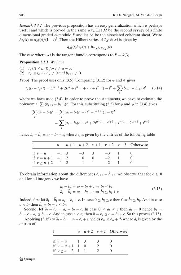
Remark 3.3.2 The previous proposition has an easy generalization which is perhapsuseful and which is proved in the same way. Let M be the second syzygy of a finitedimensional graded A-module F and let M be the associated coherent sheaf. WritehM(t) = qM(t)/(1 − t)3. Then the Hilbert series of IX ⊗ M is given by
qM(t)hIX (t)+ hTorA1 (F,IX )
(t)
The case where M is the tangent bundle corresponds to F = k(3).
Proposition 3.3.3 We have
(1) tψ(l) ≤ tϕ(l) for l = u − 3, v(2) tψ ≤ tϕ ⇔ au = 0 and bv+3 = 0
Proof The proof uses only (3.5). Comparing (3.12) for ϕ and ψ gives
tϕ(t)− tψ(t) = 3tu−1 + 2(tu + tu+1 + · · · + tv−1)− tv +∑
i
(bi+3 − bi+3)ti (3.14)
where we have used (3.4). In order to prove the statements, we have to estimate thepolynomial
∑i(bi+3 − bi+3)ti. For this, substituting (2.2) for ϕ and ψ in (3.4) gives
∑
i
(ai − bi)ti =∑
i
(ai − bi)ti − (tu − tv+1)(1 − t)2
=∑
i
(ai − bi)ti − tu + 2tu+1 − tu+2 + tv+1 − 2tv+2 + tv+3
hence al − bl = al − bl + el where el is given by the entries of the following table
l u u + 1 u + 2 v + 1 v + 2 v + 3 Otherwise
if v = u −1 3 −3 3 −3 1 0if v = u + 1 −1 2 0 0 −2 1 0if v ≥ u + 2 −1 2 −1 1 −2 1 0
To obtain information about the differences bi+3 − bi+3, we observe that for c ≥ 0and for all integers l we have
al − bl = al − bl + c ⇒ bl ≤ bl
al − bl = al − bl − c ⇒ bl ≤ bl + c(3.15)
Indeed, first let al − bl = al − bl + c. In case 0 ≤ bl ≤ c then 0 = bl ≤ bl. And in casec < bl then bl = bl − c ≤ bl.
Second, let al − bl = al − bl − c. In case 0 ≤ al ≤ c then al = 0 hence bl =bl + c − al ≤ bl + c. And in case c < al then 0 = bl ≤ c = bl + c. So this proves (3.15).
Applying (3.15) to al − bl = al − bl + el yields bu ≤ bu + dl where dl is given by theentries of
l u u + 2 v + 2 Otherwise
if v = u 1 3 3 0if v = u + 1 1 0 2 0if v ≥ u + 2 1 1 2 0

On incidence between strata of the Hilbert scheme of points on P2 909
Now we are able to prove the first statement. Combining bu ≤ bu +dl and (3.14) gives
tϕ(t)− tψ(t) ≥⎧⎨
⎩
−tu−3 − tv if v = u−tu−3 + 3tu−1 − tv if v = u + 1−tu−3 + 2(tu−1 + tu + · · · + tv−2)− tv if v ≥ u + 2
(3.16)
and therefore tϕ(t)−tψ(t) ≥ −tu−3−tv which concludes the proof of the first statement.For the second part, assume that tψ ≤ tϕ . Equation (3.14) implies that
bu ≤ bu
bv+3 ≤ bv+3 − 1(3.17)
Since bv+3 ≥ 0 we clearly have bv+3 > 0. Assume, by contradiction, that au = 0. Fromal − bl = al − bl + el we have au − bu = au − bu − 1 hence au = 0 and bu = bu + 1.But this gives a contradiction with (3.17). Therefore
tψ ≤ tϕ ⇒ au > 0 and bv+3 > 0
To prove the converse let au > 0 and bv+3 > 0. Due to the first part we only need toprove that tψ(u − 3) ≤ tϕ(u − 3) and tψ(v) ≤ tϕ(v). Equation (3.14) gives us
tϕ(u − 3)− tψ(u − 3) = bu − bu
tϕ(v)− tψ(v) = bv+3 − bv+3 − 1 (3.18)
while from al − bl = al − bl + el we have
au − bu = au − bu − 1
av+3 − bv+3 = av+3 − bv+3 + 1
Since au > 0, bv+3 > 0 we have bu = 0, av+3 = 0 hence
au − bu = au − 1
av+3 − bv+3 = −bv+3 + 1
which implies au − bu ≥ 0, av+3 − bv+3 ≤ 0 hence bu = 0, av+3 = 0. Thus bu = bu = 0and bv+3 = bv+3 − 1. Combining with (3.18) this proves that tϕ(u − 3) = tψ(u − 3) andtϕ(v) = tψ(v), finishing the proof. ��
3.4 Combining everything
In this section we prove that Condition B implies Condition C. So assume that Con-dition B holds.
Since the tangent condition holds we have by Proposition 3.3.3
au = 0 and bv+3 = 0
This means there is nothing to prove if u = v. So assume that v ≥ u + 1. Sincethe dimension condition holds, Corollary 3.2.2 implies Condition C. This finishes theproof.

910 K. De Naeghel, M. Van den Bergh
Remark 3.4.1 By the above results it is easy to see that Condition C implies ConditionB, where in case v ≥ u + 1 one makes use of Corollary 3.2.2. This gives a direct proofof the implication C ⇒ B (i.e. without going through the other conditions).
Remark 3.4.2 The reader will have noticed that our proof of the implication B ⇒ Cis rather involved. Since the equivalence of B and C is purely combinatorial it can bechecked directly for individual n. Using a computer we have verified the equivalenceof B and C for n ≤ 70.
Remark 3.4.3 The reader may observe that in case v = u we have
tψ ≤ tϕ ⇒ dim Hϕ < dim Hψ (3.19)
while if v ≥ u + 2 we have
dim Hϕ < dim Hψ ⇒ tψ ≤ tϕ (3.20)
It is easy to construct counter examples which show that the reverse implications donot hold, and neither (3.19) nor (3.20) is valid in case v = u + 1.
4 The implication C ⇒ D
In this section (ϕ,ψ) will have the same meaning as in Sect. 3 and we also keep theassociated notations.
4.1 Truncated point modules
A truncated point module of length m is a graded A-module generated in degree zerowith Hilbert series 1 + t + · · · + tm−1.
If F is a truncated point module of length > 1 then there are two independenthomogeneous linear forms l1, l2 vanishing on F and their intersection defines a pointp ∈ P
2. We may choose basis vectors ei ∈ Fi such that
xei = xpei+1, yei = ypei+1, zei = zpei+1
where (xp, yp, zp) is a set of homogeneous coordinates of p. It follows that if f ∈ A ishomogeneous of degree d and i + d ≤ m − 1 then
fei = fpei+d
where (−)p stands for evaluation in p (with respect to the homogeneous coordinates(xp, yp, zp)).
If G = ⊕iA(−i)ci then we have
HomA(G, F) = ⊕0≤i≤m−1Fcii
∼= k∑
0≤i≤m−1 ci (4.1)
where the last identification is made using the basis (ei)i introduced above.

On incidence between strata of the Hilbert scheme of points on P2 911
In the sequel we will need the minimal projective resolution of a truncated pointmodule F of length m. It is easy to see that it is given by
0 → A(−m − 2)
⎛
⎜⎜⎝
l1l2ρ
⎞
⎟⎟⎠
−−−→f3
A(−m − 1)2 ⊕ A(−2)
⎛
⎜⎜⎝
0 −ρ l2ρ 0 −l1
−l2 l1 0
⎞
⎟⎟⎠
−−−−−−−−−−−→f2
A(−1)2
⊕ A(−m)
(l1 l2 ρ
)
−−−−−−→f1
A → F → 0 (4.2)
where l1, l2 are the linear forms vanishing on F and ρ is a form of degree m such thatρp = 0 for the point p corresponding to F. Without loss of generality we may and wewill assume that ρp = 1.
4.2 A complex whose homology is J
In this section I is a graded ideal corresponding to a generic point in Hϕ . The followinglemma gives the connection between truncated point modules and Condition D.
Lemma 4.2.1 If an ideal J ⊂ I has Hilbert series hA − ψ then I/J is a (shifted bygrading) truncated point module of length v + 1 − u.
Proof Since F = I/J has the correct (shifted) Hilbert function, it is sufficient to showthat F is generated in degree u.
If v = u then there is nothing to prove. If v ≥ u + 1 then by Proposition 3.1.1 thegenerators of I are in degrees ≤ u and ≥ v + 2. Since F lives in degrees u, . . . , v thisproves what we want. ��
Let J, F be as in the previous lemma. Below we will need a complex whose homol-ogy is J. We write the minimal resolution of F as
0 → G3f3−→ G2
f2−→ G1f1−→ G0 −→ F → 0
where the maps fi are as in (4.2), and the minimal resolution of I as
0 → F1 → F0 → I → 0
The map I → F induces a map of projective resolutions
0 −−−−−→ F1M−−−−−→ F0 −−−−−→ I −−−−−→ 0
γ1
⏐⏐� γ0
⏐⏐�
⏐⏐�
0 −−−−−→ G3f3−−−−−→ G2
f2−−−−−→ G1f1−−−−−→ G0
f0−−−−−→ F −−−−−→ 0
(4.3)
Taking cones yields that J is the homology at G1 ⊕ F0 of the following complex
0 → G3
(f30
)
−−−→ G2 ⊕ F1
(f2 γ10 −M
)
−−−−−−−−→ G1 ⊕ F0
(f1 γ0
)
−−−−−−→ G0 → 0 (4.4)
Note that the rightmost map is split here. By selecting an explicit splitting we mayconstruct a free resolution of J, but it will be convenient not to do this.

912 K. De Naeghel, M. Van den Bergh
For use below we note that the map J → I is obtained from taking homology ofthe following map of complexes.
0 �� G3
(f30
)
�� G2 ⊕ F1(0 −1
)
��
(f2 γ10 −M
)
�� G1 ⊕ F0(0 1
)
��
(f1 γ0
)
�� G0 �� 0
0 �� F1 M�� F0 �� 0
(4.5)
4.3 The Hilbert scheme of an ideal
In this section I is a graded ideal corresponding to a generic point in Hϕ .Let V be the Hilbert scheme of graded quotients F of I with Hilbert series tu+· · ·+tv.
To see that V exists one may realize it as a closed subscheme of
Proj S(Iu ⊕ · · · ⊕ Iv)
where SV is the symmetric algebra of a vector space V. Alternatively see [1,9].We will give an explicit description of V by equations. Here and below we use
the following convention: if N is a matrix with coefficients in A representing a map⊕jA(−j)dj → ⊕iA(−i)ci then N(p, q) stands for the submatrix of N representing theinduced map A(−q)dq → A(−p)cp .
We now distinguish two cases.
v = u In this case it is clear that V ∼= Pau−1.
v ≥ u + 1 Let F ∈ V and let p ∈ P2 be the associated point. Let (ei)i be a basis for F
as in Sect. 4.1. The map I → F defines a map
λ : A(−u)au → F
such that the composition
A(−u − 1)bu+1M(u,u+1)·−−−−−−→ A(−u)au → F (4.6)
is zeroWe may view λ as a scalar row vector as in (4.1). The fact that (4.6) haszero composition then translates into the condition
λ · M(u, u + 1)p = 0 (4.7)
It is easy to see that this procedure is reversible and that the equations(4.7) define V as a subscheme of P
au−1 × P2.
Proposition 4.3.1 Assume that Condition C holds. Then V is smooth and
dim V ={
au − 1 if v = u
au + 1 − bu+1 if v ≥ u + 1
Proof The case v = u is clear so assume v ≥ u + 1. If we look carefully at (4.7)then we see that it describes V as the zeroes of bu+1 generic sections of the veryample line bundle O
Pau−1(1)� O
P2(1) on P
au−1 × P2. It follows from Condition C that
On incidence between strata of the Hilbert scheme of points on P2 913
bu+1 ≤ dim(P2 × Pau−1) = au + 1. Hence by Bertini (see [13]) we deduce that V is
smooth of dimension au + 1 − bu+1. ��
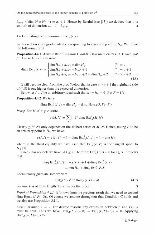
4.4 Estimating the dimension of Ext1A(J, J)
In this section I is a graded ideal corresponding to a generic point of Hϕ . We provethe following result
Proposition 4.4.1 Assume that Condition C holds. Then there exists F ∈ V such thatfor J = ker(I → F) we have
dimk Ext1A(J, J) ≥
⎧⎪⎨
⎪⎩
dim Hψ + av+3 = dim Hψ if v = u
dim Hψ + av+2 − bv+3 + 1 if v = u + 1dim Hψ + av+2 − bv+3 + 2 = dim Hψ + 2 if v ≥ u + 2
(4.8)
It will become clear from the proof below that in case v ≥ u + 1 the righthand sideof (4.8) is one higher than the expected dimension.
Below let J ⊂ I be an arbitrary ideal such that hJ = hA − ψ . Put F = I/J.
Proposition 4.4.2 We have
dimk Ext1A(J, J) = dim Hψ + dimk HomA(J, F(−3))
Proof For M, N ∈ gr A write
χ(M, N) =∑
i
(−1)i dimk ExtiA(M, N)
Clearly χ(M, N) only depends on the Hilbert series of M, N. Hence, taking J′ to bean arbitrary point in Hψ we have
χ(J, J) = χ(J′, J′) = 1 − dimk Ext1A(J
′, J′) = 1 − dim Hψ
where in the third equality we have used that Ext1A(J
′, J′) is the tangent space toHψ [7].
Since J has no socle we have pd J ≤ 2. Therefore ExtiA(J, J) = 0 for i ≥ 3. It follows
that
dimk Ext1A(J, J) = −χ(J, J)+ 1 + dimk Ext2
A(J, J)
= dim Hψ + dimk Ext3A(F, J)
Local duality gives an isomorphism
Ext3A(F, J)∗ ∼= HomA(J, F(−3)) (4.9)
because F is of finite length. This finishes the proof. ��Proof of Proposition 4.4.1 It follows from the previous result that we need to controldimk HomA(J, F(−3)). Of course we assume throughout that Condition C holds andwe also use Proposition 3.1.1.
Case 1 Assume v = u. For degree reasons any extension between F and F(−3)must be split. Thus we have HomA(F, F(−3)) = Ext1
A(F, F(−3)) = 0. ApplyingHomA(−, F(−3)) to

914 K. De Naeghel, M. Van den Bergh
0 → J → I → F → 0
we find
HomA(J, F(−3)) = HomA(I, F(−3))
Hence
dimk HomA(J, F(−3)) = av+3 = 0
Case 2 Assume v = u + 1. As in the previous case we find HomA(J, F(−3)) =HomA(I, F(−3)).
Thus a map J → F(−3) is now given (using Proposition 3.1.1) by a map
β : A(−v − 2)av+2 → F(−3)
(identified with a scalar vector as in (4.1)) such that the composition
A(−v − 3)bv+3M(v+2,v+3)−−−−−−−→ A(−v − 2)av+2
β−→ F(−3)
is zero. This translates into the condition
β · M(v + 2, v + 3)p = 0 (4.10)
where p is the point corresponding to F. Now M(v + 2, v + 3) is a av+2 × bv+3 matrix.Since bv+3 ≤ av+2 (by Proposition 3.1.1) we would expect (4.10) to have av+2 − bv+3independent solutions. To have more, M(v + 2, v + 3) has to have non-maximal rank.I.e. there should be a non-zero solution to the equation
M(v + 2, v + 3)p · δ = 0 (4.11)
This should be combined with (see (4.7))
λ · M(u, u + 1)p = 0 (4.12)
We view (4.11) and (4.12) as a system of av+2 + bu+1 equations inP
au−1 × P2 × P
bv+3−1. Since (Condition C)
av+2 + bu+1 ≤ dim(Pau−1 × P2 × P
bv+3−1) = au + bv+3
the system (4.11)(4.12) has a solution provided the divisors in Pau−1 × P
2 × Pbv+3−1
determined by the equations of the system have non-zero intersection product.Let r, s, t be the hyperplane sections in P
au−1, P2 and P
bv+3−1, respectively. TheChow ring of P
au−1 × P2 × P
bv+3−1 is given by
Z[r, s, t]/(rau , s3, tbv+3) (4.13)
The intersection product we have to compute is
(s + t)av+2(r + s)bu+1
This product contains the terms
tav+2−2s2rbu+1
tav+2−1s2rbu+1−1
tav+2 s2rbu+1−2
at least one of which is non-zero in (4.13) (using Condition C).
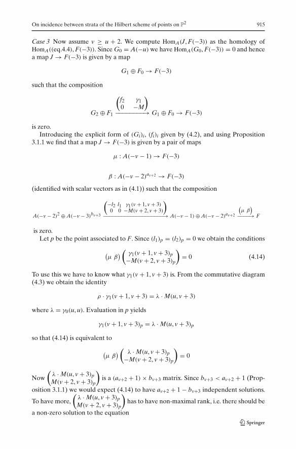
On incidence between strata of the Hilbert scheme of points on P2 915
Case 3 Now assume v ≥ u + 2. We compute HomA(J, F(−3)) as the homology ofHomA((eq.4.4), F(−3)). Since G0 = A(−u) we have HomA(G0, F(−3)) = 0 and hencea map J → F(−3) is given by a map
G1 ⊕ F0 → F(−3)
such that the composition
G2 ⊕ F1
(f2 γ10 −M
)
−−−−−−−−→ G1 ⊕ F0 → F(−3)
is zero.Introducing the explicit form of (Gi)i, (fi)i given by (4.2), and using Proposition
3.1.1 we find that a map J → F(−3) is given by a pair of maps
μ : A(−v − 1) → F(−3)
β : A(−v − 2)av+2 → F(−3)
(identified with scalar vectors as in (4.1)) such that the composition
A(−v − 2)2 ⊕ A(−v − 3)bv+3
(−l2 l1 γ1(v + 1, v + 3)0 0 −M(v + 2, v + 3)
)
−−−−−−−−−−−−−−−−−−−−→ A(−v − 1)⊕ A(−v − 2)av+2
(μ β
)
−−−−→ F
is zero.Let p be the point associated to F. Since (l1)p = (l2)p = 0 we obtain the conditions
(μ β
)(γ1(v + 1, v + 3)p
−M(v + 2, v + 3)p
)
= 0 (4.14)
To use this we have to know what γ1(v + 1, v + 3) is. From the commutative diagram(4.3) we obtain the identity
ρ · γ1(v + 1, v + 3) = λ · M(u, v + 3)
where λ = γ0(u, u). Evaluation in p yields
γ1(v + 1, v + 3)p = λ · M(u, v + 3)p
so that (4.14) is equivalent to
(μ β
)(λ · M(u, v + 3)p
−M(v + 2, v + 3)p
)
= 0
Now(λ · M(u, v + 3)pM(v + 2, v + 3)p
)
is a (av+2 + 1)× bv+3 matrix. Since bv+3 < av+2 + 1 (Prop-
osition 3.1.1) we would expect (4.14) to have av+2 + 1 − bv+3 independent solutions.
To have more,(λ · M(u, v + 3)pM(v + 2, v + 3)p
)
has to have non-maximal rank, i.e. there should be
a non-zero solution to the equation
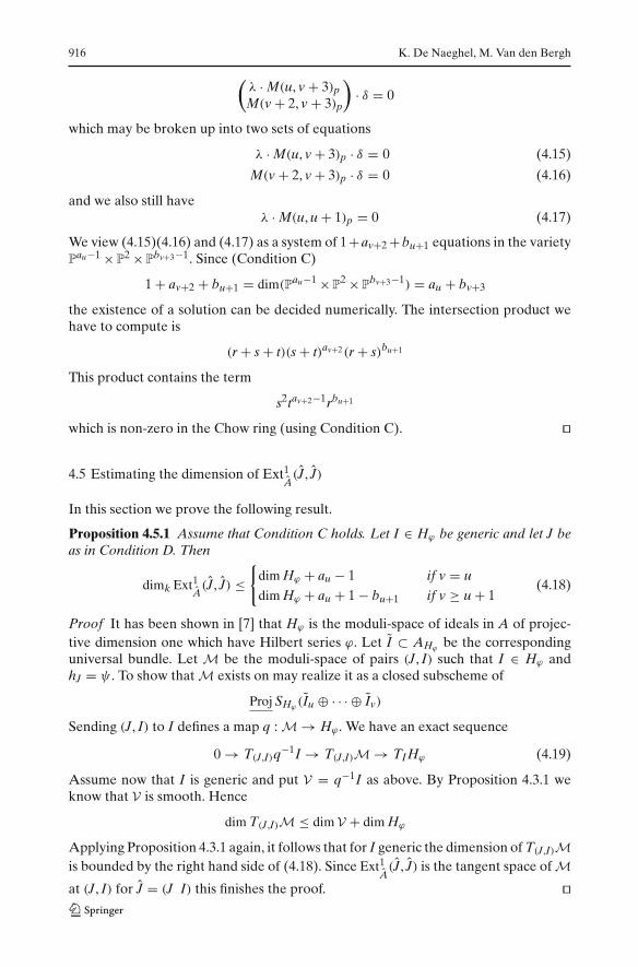
916 K. De Naeghel, M. Van den Bergh
(λ · M(u, v + 3)pM(v + 2, v + 3)p
)
· δ = 0
which may be broken up into two sets of equations
λ · M(u, v + 3)p · δ = 0 (4.15)
M(v + 2, v + 3)p · δ = 0 (4.16)
and we also still haveλ · M(u, u + 1)p = 0 (4.17)
We view (4.15)(4.16) and (4.17) as a system of 1+av+2 +bu+1 equations in the varietyP
au−1 × P2 × P
bv+3−1. Since (Condition C)
1 + av+2 + bu+1 = dim(Pau−1 × P2 × P
bv+3−1) = au + bv+3
the existence of a solution can be decided numerically. The intersection product wehave to compute is
(r + s + t)(s + t)av+2(r + s)bu+1
This product contains the term
s2tav+2−1rbu+1
which is non-zero in the Chow ring (using Condition C). ��
4.5 Estimating the dimension of Ext1A(J, J)
In this section we prove the following result.
Proposition 4.5.1 Assume that Condition C holds. Let I ∈ Hϕ be generic and let J beas in Condition D. Then
dimk Ext1A(J, J) ≤
{dim Hϕ + au − 1 if v = u
dim Hϕ + au + 1 − bu+1 if v ≥ u + 1(4.18)
Proof It has been shown in [7] that Hϕ is the moduli-space of ideals in A of projec-tive dimension one which have Hilbert series ϕ. Let I ⊂ AHϕ
be the correspondinguniversal bundle. Let M be the moduli-space of pairs (J, I) such that I ∈ Hϕ andhJ = ψ . To show that M exists on may realize it as a closed subscheme of
Proj SHϕ(Iu ⊕ · · · ⊕ Iv)
Sending (J, I) to I defines a map q : M → Hϕ . We have an exact sequence
0 → T(J,I)q−1I → T(J,I)M → TIHϕ (4.19)
Assume now that I is generic and put V = q−1I as above. By Proposition 4.3.1 weknow that V is smooth. Hence
dim T(J,I)M ≤ dim V + dim Hϕ
Applying Proposition 4.3.1 again, it follows that for I generic the dimension of T(J,I)Mis bounded by the right hand side of (4.18). Since Ext1
A(J, J) is the tangent space of M
at (J, I) for J = (J I) this finishes the proof. ��

On incidence between strata of the Hilbert scheme of points on P2 917
Remark 4.5.2 It is not hard to see that (4.18) is actually an equality. This follows fromthe easily proved fact that the map q is generically smooth.
4.6 Tying things together
Combining the results of the previous two sections we see that if Condition C holdswe have for a suitable choice of J
dimk Ext1A(J, J)− dimk Ext1
A(J, J)
≥
⎧⎪⎨
⎪⎩
dim Hψ − dim Hϕ + av+3 − au + 1 if v = u
dim Hψ − dim Hϕ + av+2 − bv+3 − au + bu+1 if v = u + 1dim Hψ − dim Hϕ + av+2 − bv+3 − au + bu+1 + 1 if v ≥ u + 2
We may combine this with Proposition 3.2.1 which by au > 0, bv+3 > 0 (Condition C)works out as
dim Hψ − dim Hϕ =
⎧⎪⎨
⎪⎩
au + bv+3 − 1 if v = u
au − bu+1 − av+2 + bv+3 + 1 if v = u + 1au − bu+1 − av+2 + bv+3 if v ≥ u + 2
We then obtain
dimk Ext1A(J, J)− dimk Ext1
A(J, J) ≥
{bv+3 if v = u
1 if v ≥ u + 1
Hence in all cases we obtain a strictly positive result. This finishes the proof thatCondition C implies Condition D.
Remark 4.6.1 As in Remark 3.4.1 it is possible to prove directly the converse impli-cation D ⇒ C.
5 The implication D ⇒ A
In this section (ϕ,ψ) will have the same meaning as in Sect. 3 and we also keep theassociated notations. We assume that Condition D holds. Let I be a graded ideal cor-responding to a generic point in Hϕ . According to Condition D there exists an idealJ ⊂ I with hJ = ψ such that there is an η ∈ Ext1
A(J, J) which is not in the image ofExt1
A(J, J).
We identify η with a one parameter deformation J′ of J. I.e. J′ is a flat A[ε]-modulewhere ε2 = 0 such that J′ ⊗k[ε] k ∼= J and such that the short exact sequence
0 → Jε·−→ J′ → J → 0
corresponds to η.In Sect. 4.2 we have written J as the homology of a complex. It follows for example
from (the dual version of) [15, Theorem 3.9], or directly, that J′ is the homology of a

918 K. De Naeghel, M. Van den Bergh
complex of the form
0 → G3[ε]
(f ′3
Pε
)
−−−−→ G2[ε] ⊕ F1[ε]
(f ′2 γ ′
1Qε −M′
)
−−−−−−−−→ G1[ε] ⊕ F0[ε](f ′1 γ
′0
)
−−−−−→ G0[ε] → 0
(5.1)
where for a matrix U over A, U′ means a lift of U to A[ε]. Recall that G3 = A(−v−3).
Lemma 5.1 We have P(v + 3, v + 3) = 0.
Proof Assume on the contrary P(v + 3, v + 3) = 0. Using Proposition 3.1.1 it followsthat P has its image in F11 = ⊕j≤u+1A(−j)bj .
The fact that (5.1) is a complex implies that Qf3 = MP. Thus we have a commutativediagram
0 −−−−→ G3f3−−−−→ G2
f2−−−−→ G1f1−−−−→ G0
P1
⏐⏐�
⏐⏐�Q
F11M11−−−−→ F0
P2
⏐⏐�
∥∥∥
F1 −−−−→M
F0
where P2 is the inclusion and M11 = MP2, P = P2P1. Put
D = coker(F11 → F1)
Then (P1, Q) represents an element of Ext2A(F, D) ∼= Ext1
A(D, F(−3))∗ = 0, wherethe isomorphism is obtained by same arguments as (4.9), and the last equality is fordegree reasons. It follows that there exist maps
R : G1 → F0
T1 : G2 → F11
such that
Q = Rf2 + M11T1
P1 = T1f3
Putting T = P2T1 we obtain
Q = Rf2 + MT
P = Tf3
We can now construct the following lifting of the commutative diagram (4.5):
0 �� G3[ε]
(f ′3Pε
)
�� G2[ε] ⊕ F1[ε](Tε −1
)
��
(f ′2 γ ′
1Qε −M′
)
�� G1[ε] ⊕ F0[ε](−Rε 1
)
��
(f ′1 γ ′
0
)
�� G0[ε] �� 0
0 �� F1[ε]M′+Rγ1ε
�� F0[ε] �� 0

On incidence between strata of the Hilbert scheme of points on P2 919
Taking homology we see that there is a first order deformation I′ of I together with alift of the inclusion J → I to a map J′ → I′. But this contradicts the assumption thatη is not in the image of Ext1
A(J, J). ��
In particular, Lemma 5.1 implies that bv + 3 = 0. It will now be convenient torearrange (5.1). Using the previous lemma and the fact that the rightmost map in(5.1) is split it follows that J′ has a free resolution of the form
0 → G3[ε]
(ε
α0 + α1ε
)
−−−−−−−−→ G3[ε] ⊕ H1[ε](β0 + β1ε δ0 + δ1ε
)
−−−−−−−−−−−−−−−−→ H0[ε] → J′ → 0
which leads to the following equations
δ0α0 = 0
β0 + δ1α0 + δ0α1 = 0
Using these equations we can construct the following complex Ct over A[t]
0 → G3[t]
(t
α0 + α1t
)
−−−−−−−−→ G3[t] ⊕ H1[t](β0 − δ1α1t δ0 + δ1t
)
−−−−−−−−−−−−−−−→ H0[t]
For θ ∈ k put Cθ = C ⊗k[t] k[t]/(t − θ). Clearly C0 is a resolution of J. By semi-con-tinuity we find that for all but a finite number of θ , Cθ is the resolution of a rank oneA-module Jθ . Furthermore we have J0 = J and pd Jθ = 1 for θ = 0.
Let Jθ be the rank one OP
2 -module corresponding to Jθ . Jθ represents a pointof Hψ . Since I/J has finite length, J0 = J and I define the same object in Hilbn(P
2).Hence we have constructed a one parameter family of objects in Hilbn(P
2) connectinga generic object in Hϕ to an object in Hψ . This shows that indeed Hϕ is in the closureof Hψ .
Appendix A. Hilbert graphs
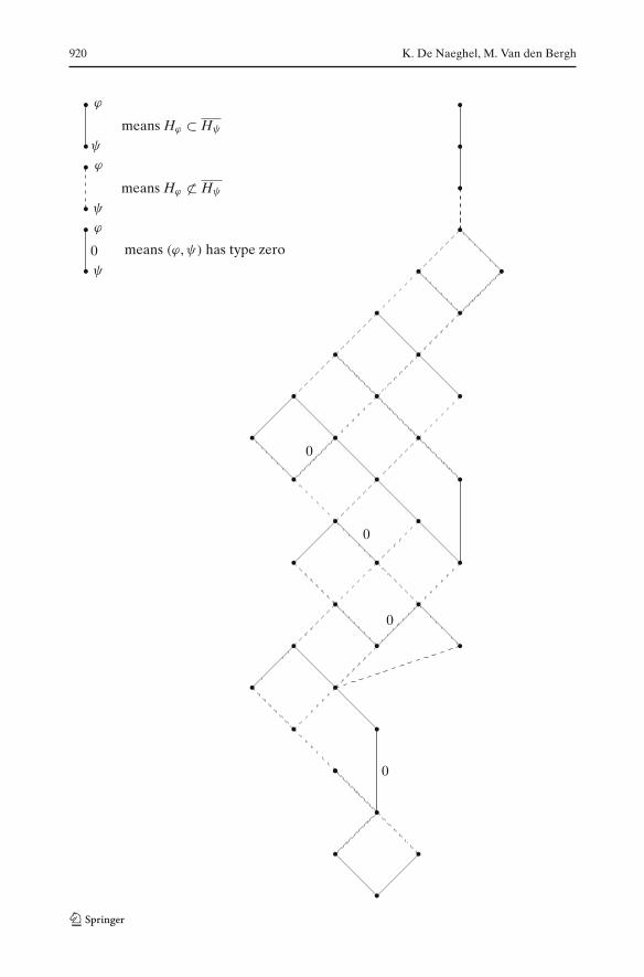
For low values of n the Hilbert graph is rather trivial. But when n becomes biggerthe number of Hilbert functions increase rapidly (see Remark 1.3) and so the Hil-bert graphs become more complicated. As an illustration we have included the Hilbertgraph for n = 17 where we used Theorem 1.5 to solve the incidence problems of lengthzero (the picture gives no information on more complicated incidence problems). Byconvention the minimal Hilbert series is on top.
The reader will notice that the Hilbert graph contains pentagons. This shows thatthe Hilbert graph is not catenary and also contradicts [12, Lemma 2.1.2].
920 K. De Naeghel, M. Van den Bergh
means Hϕ ⊂ Hψ
means Hϕ ⊂ Hψ
means (ϕ,ψ) has type zero
ϕ
ψ
0
0
0
0
0
ϕ
ϕ
ψ
ψ
�
�
�
�
� �
� �
� �
� � �
� � �
� � �
� �
� � �
� �
� � �
� �
� �
��
�
� �
�
�
�
�
�
�
�

On incidence between strata of the Hilbert scheme of points on P2 921
Appendix B. A visual criterion for incidence problems of length zero
In this appendix we provide a visual criterion for the three conditions in Theorem 1.5.The reader may easily check these using Condition C, Propositions 3.1.1 and (3.2).As before we let (ϕ,ψ) be a pair of Hilbert series of degree n and length zero. ThenHϕ ⊂ Hψ if and only if the Castelnuovo diagram sϕ of ϕ has one of the followingforms, where the diagram sψ is obtained by moving the upper square as indicated.
��≥ 0
����
��
C ≥ 1
D ≥ 0where C > D
≥ 1
��2
��≥ 0
����
C ≥ 1
D ≥ 0where C > D
����
A ≥ 0
B ≥ 1where A < B
��≥ 1
��≥ 1
��
��≥ 2
≥ 0
≥ 1
��3
��
��≥ 0
��3
�
�
��≥ 1
≥ 2
��≥ 2
≥ 1
��3
��
��
≥ 1
��≥ 2
��
��≥ 2
≥ 0
≥ 1��
��≥ 4
References
1. Artin, M., Zhang, J.: Abstract Hilbert schemes. Algebr. Represent. Theory 4(4), 305–394 (2001)2. Brun, J., Hirschowitz, A.: Le problème de Brill-Noether pour les idéaux de P
2. Ann. Sci. ÉcoleNorm. Sup. 20(4)(2), 171–200 (1987)
3. Coppo, M.A.: Familles maximales de systèmes de points surabondants dans le plan projectif.Math. Ann. 291(4), 725–735 (1991)
4. Coppo, M.A., Walter, C.: Composante centrale du lieu de Brill-Noether de Hilb2(P2). Lect. NotesPure Appl. Math., vol. 200, 341–349, Dekker, New-York, 1998.
5. Davis, E.D.: 0-dimensional subschemes of P2: new application of Castelnuovo’s function. Ann.
Univ. Ferrara 32, 93–107 (1986)6. De Naeghel, K., Van den Bergh, M.: Ideal classes of three-dimensional Sklyanin algebras.
J. Algebra 276, 515–551 (2004)
922 K. De Naeghel, M. Van den Bergh
7. De Naeghel, K., Van den Bergh, M.: Ideal classes of three dimensional Artin-Schelter regularalgebras. J. Algebra 283(1), 399–429 (2005)
8. Geramita, A.V., Maroscia, P., Roberts, L.G.: The Hilbert function of a reduced k-algebra. J. Lond.Math. Soc. (2) 28(3), 443–452 (1983)
9. Gotzmann, G.: Eine Bedingung für die Flachheit und das Hilbertpolynom eines graduiertenRinges. Math. Z. 158(1), 61–70 (1978)
10. Gotzmann, G.: A stratification of the Hilbert scheme of points on the projective plane. Math. Z.199(4), 539–547 (1988)
11. Gruson, L., Peskine, C.: Genre des courbes de l’espace projectif. Lecture notes in Mathematics,vol. 687, pp. 31–59, Springer, Berlin Heidelberg New York 1978
12. Guerimand, F.: Sur l’incidence des strates de Brill-Noether du schéma de Hilbert des points duplan projectif. Ph.D. thesis, Université de Nice, Sophia Antipolis, 2002
13. Hartshorne, R.: Algebraic geometry. Springer, Berlin Heidelberg New York 197714. Hirschowitz, A., Rahavandrainy, O., Walter, C.: Quelques strates de Brill-Noether du schéma de
Hilbert de P2. C. R. Acad. Sci. Paris, Sér. I Math. 319(6), 589–594 (1994)
15. Lowen, W.: Obstruction theory for objects in abelian and derived categories. Comm. Algebra33(9), 3195–3223 (2005)
16. Nevins, T.A., Stafford, J.T.: Sklyanin algebras and Hilbert schemes of points. preprint math.AG/0310045, 2003