on an extreme value version of the … · on an extreme value version of the birnbaum–saunders...

REVSTAT – Statistical Journal

Volume 10, Number 2, June 2012, 181–210

ON AN EXTREME VALUE VERSION OF THE

BIRNBAUM–SAUNDERS DISTRIBUTION

Authors: Marta Ferreira

– Departamento de Matematica, Universidade do Minho,Braga, [email protected]

M. Ivette Gomes

– D.E.I.O. (F.C.U.L.) and C.E.A.U.L., Universidade de Lisboa,Lisboa, [email protected]

Vıctor Leiva

– Departamento de Estadıstica, Universidad de Valparaıso,Valparaıso, [email protected]

Received: September 2011 Revised: November 2011 Accepted: November 2011

Abstract:

• The Birnbaum–Saunders model is a life distribution originated from a problem of ma-terial fatigue that has been largely studied and applied in recent decades. A randomvariable following the Birnbaum–Saunders distribution can be stochastically repre-sented by another random variable used as basis. Then, the Birnbaum–Saundersmodel can be generalized by switching the distribution of the basis variable using di-verse arguments allowing to construct more general classes of models. Extreme valuedistributions are useful to determinate the probability of events that are larger orsmaller than others previously observed. In this paper, we propose, characterize, im-plement and apply an extreme value version of the Birnbaum–Saunders distribution.

Key-Words:

• domain of attraction; extreme data; likelihood method; R computer language.

AMS Subject Classification:

• 60E05, 62G32, 62N02, 62N99.

182 Marta Ferreira, M. Ivette Gomes and Vıctor Leiva

On an Extreme Value Version of the Birnbaum–Saunders Distribution 183

1. INTRODUCTION

Extreme value (EV) models are appropriate to establish the probability of

events that are larger or smaller than others previously observed. As an example

where these models can be used, suppose that a sea-wall projection requires a

coastal defence from all sea levels for the next 100 years. These EV models are

a precious tool that enables this type of extrapolations. Actually, the EV theory

is widely used by many researchers in applied sciences when high values of cer-

tain phenomena are modeled. For instance, ocean wave, thermodynamics of

earthquakes, wind energy, risk assessment on financial markets, and medical phe-

nomena can be mentioned. Some books on EV theory are Leadbetter et al.

(1983), Galambos (1987), Embrechts et al. (1997), Beirlant et al. (2004), and

de Haan and Ferreira (2006). For a more practical view on this topic, see Coles

(2001), and for more recent references, see Ferreira and Canto e Castro (2008),

Gomes et al. (2008a,b), Beirlant et al. (2012), and Scarrot and MacDonald (2012),

among others.

Life distributions are usually positively skewed, unimodal, two-parameter

models and with non-negative support; see Marshall and Olkin (2007) and Saun-

ders (2007). A life distribution that has received a considerable attention in recent

decades is the Birnbaum–Saunders (BS) model. This model was originated from a

problem of material fatigue and has been largely applied to reliability and fatigue

studies; see Birnbaum and Saunders (1969). The BS distribution relates the total

time until the failure to some type of cumulative damage normally distributed.

This attention for the BS distribution is due to its many attractive properties

and its relationship with the normal distribution.

Extensive work has been done on the BS model with regard to its properties,

inference and applications. A comprehensive treatment on this model until mid

90’s can be found in Johnson et al. (1995, pp. 651–662). For more detail about

new applications of the BS model, see Leiva et al. (2009a). For applications in

fields beyond engineering allowing business, environmental and medical data to

be analyzed by using this model, see Leiva et al. (2007, 2008b, 2009b, 2010a,b,

2011), Podlaski (2008), Barros et al. (2008), Bhatti (2010), Ahmed et al. (2010),

and Vilca et al. (2010). Thus, at the present, the BS model can be widely used

as a statistical distribution rather than restricted to a life distribution.

Because a random variable (r.v.) following the BS distribution can be repre-

sented by another basis r.v., generalizations of this distribution can be obtained

switching the distribution of the basis variable by diverse arguments allowing

to construct more general classes of models. Several generalizations of the BS

distribution have been recently proposed by a number of authors, including Dıaz-

Garcıa and Leiva (2005), Vilca and Leiva (2006), Sanhueza et al. (2008), Gomez

et al. (2009) and Guiraud et al. (2009), which allow us to obtain a major degree of


flexibility for this distribution. Usual and generalized versions of the BS distribu-

tion are implemented in the R software (http://www.R-project.org) by packages

called bs and gbs, which can be downloaded from http://CRAN.R-project.org;

see Leiva et al. (2006) and Barros et al. (2009). These packages contain functions

for computing probabilities, estimating parameters, generating random numbers

and carrying out goodness-of-fit and hazard analysis. Leiva et al. (2008a) stud-

ied three generators of random numbers from the BS and generalized BS (GBS)

distributions.

The main aim of this work is to obtain an EV version of the BS distribution

relevant not only by itself as a model, but also for a parametric statistical anal-

ysis of extreme or rare events. The paper is organized as follows. In Section 2,

we provide a preliminary notion of different aspects related to BS and EV distri-

butions. In Section 3, we characterize extreme value Birnbaum–Saunders (EVBS)

distributions. In Section 4, we focus on extremal domains of attraction of a gen-

eral class of BS models that we call BS type (BST) distributions. In Section 5,

we carry out a hazard analysis of EVBS distributions mainly based on the hazard

rate (h.r.). In Section 6, we discuss about the estimation procedure based on the

maximum likelihood (ML) method and model checking. In Section 7, we con-

duct out the numerical application of this work, which includes an exploratory

data analysis (EDA) and a parametric statistical analysis based on the EVBS

distribution. Finally, in Section 8, we sketch some concluding remarks.

2. A PRELIMINARY NOTION

In this section, we provide preliminary aspects about BS, BST and EV

distributions.

2.1. BS and BST distributions

An r.v. T with usual BS distribution is characterized by its shape and scale

parameters α > 0 and β > 0, respectively. This is denoted by T ∼ BS(α, β),

where β is also the median of the distribution. BS and standard normal r.v.’s,

denoted respectively by T and Z for now, are related by

(2.1) T = β(αZ/2 +

√{αZ/2}2 + 1

)2and Z =

(√T/β −

√β/T

)/α .

Let T ∼ BS(α, β). Then, the probability density function (p.d.f.) and cumulative

distribution function (c.d.f.) of T are respectively given by

(2.2) fT(t) = φ

(a(t)

)a′(t) and F

T(t) = Φ

(a(t)

), t > 0 ,


where φ and Φ are the standard normal p.d.f. and c.d.f., respectively,

(2.3) a(t) ≡ at =(√

t/β−√

β/t)/

α and a′(t) ≡ At = t−3/2(t+β

)/(2α

√β),

with a′(t) = da(t)/dt being the derivative of a(t) with respect to t. The quantile

function (q.f.) of T is expressed as

(2.4) t(q) ≡ tq = F−1T

(q) = β(α ξq/2 +

√{α ξq/2}2 +1

)2, 0 < q < 1 ,

where F−1T

(t) := inf{x : F (x) ≥ t} is the generalized inverse function of the c.d.f. of

T and ξq is the qth quantile of the r.v. Z ∼ N(0, 1). Note from (2.4) that, as men-

tioned, the median of T is t0.5 = β.

Important properties of T ∼ BS(α, β) are: (i) c T ∼ BS(α, c β), c > 0;

(ii) 1/T ∼ BS(α, 1/β); and (iii) V = (T/β + β/T − 2)/α2 ∼ χ2(1), i.e., V fol-

lows the χ2 distribution with one degree of freedom (d.f.).

The assumption given in (2.1) can be relaxed supposing that Z follows

any other distribution with p.d.f. fZ. Thus, we obtain the general class of BST

distributions earlier mentioned, which is denoted by T ∼ BST(α, β; fZ) for an

associated r.v. T and whose p.d.f. is given by

(2.5) fT(t) = f

Z

(a(t)

)a′(t) , t > 0 .

In particular, if Z follows a standard symmetric distribution in the real num-

ber set, denoted by Z ∼ S(fZ), we then find the GBS distribution, i.e., T ∼

GBS(α, β; g), where g is the kernel of the p.d.f. of Z given by fZ(z) = c g(z2), with

z ∈ R and c being the normalization constant, i.e., the positive value such that∫ +∞−∞ g(z2) dz = 1/c; see Dıaz-Garcıa and Leiva (2005). Then, if f

Z(z) = φ(z) =

exp(−z2/2)/√

2π, for z ∈ R, the standard normal p.d.f., we obviously recover the

usual BS distribution, i.e., an r.v. T ∼ BST(α, β; φ) ≡ BS(α, β); see Birnbaum

and Saunders (1969). For the GBS case, V = (T/β + β/T − 2)/α2 ∼ Gχ2(1; fZ),

i.e., V follows the generalized χ2 class of distributions with one d.f., which has

the χ2(1) distribution as a special case if fZ

is the standard normal density; see

Sanhueza et al. (2008).

2.2. EV distributions and extremal domains of attraction

The central limiting result in EV theory states the following. Consider an

independent identically distributed sequence of r.v.’s {Xn, n ≥ 1}, with marginal

c.d.f. F . Hence, if there are constants an > 0 and bn ∈ R, and a non-degenerate

c.d.f. G such that, as n → ∞,

P

(max{X1, ..., Xn} ≤ anx + bn

)→ G(x) ,(2.6)


then G must be the c.d.f. of a generalized extreme value (GEV) r.v., depending

on a parameter γ ∈ R. The notation X ∼ GEV(γ) is used in this case and the

corresponding c.d.f. is given by

(2.7) G(x) ≡ Gγ(x) =

{exp(−{1 + γx}−1/γ

); 1 + γx > 0, γ ∈ R\{0} ,

exp(− exp(−x)

); x ∈ R, γ = 0 ,

with G0(x) obtained from Gγ(x), for γ ∈ R\{0}, as γ → 0. As a consequence, we

say that F belongs to the max-domain of attraction of Gγ , in short F ∈ DM(Gγ).

The parameter γ, known as the EV index, is a shape parameter that determines

the right-tail behavior of F , being so a crucial parameter in EV theory. Specif-

ically, if γ < 0, we have the Weibull max-domain of attraction, i.e., light right-

tails, with a finite right endpoint. In addition, γ = 0 corresponds to the Gumbel

max-domain of attraction (exponential right-tails). And if γ > 0, we have the

Frechet max-domain of attraction corresponding to heavy right-tails (polynomial

tail decay), with an infinite right endpoint.

The GEV distribution with c.d.f. given in (2.7) is also known as the

von Mises–Jenkinson representation. This is a general form from which we derive

the three above mentioned distribution types, i.e.,

Gγ(x) =

Ψ−1/γ(−1 − γx); γ < 0 ,

Λ(x); γ = 0 ,

Φ1/γ(1 + γx); γ > 0 ,

where, for > 0, Ψ(x) = exp(−{−x}

)with x < 0 (Weibull distribution for

maxima), Λ(x) = exp(− exp(−x)

)with x ∈ R (Gumbel distribution for maxima),

and Φ(x) = exp(−x−) with x > 0 (Frechet distribution for maxima). The Gum-

bel distribution for maxima and the Frechet distribution for maxima are the com-

monly known Gumbel and Frechet distributions, respectively. Location (µ ∈ R)

and scale (σ > 0) parameters can be introduced in the GEV distribution by con-

sidering Gγ({x − µ}/σ), denoted by X ∼ GEV(µ, σ, γ).

All results developed for maxima can easily be reformulated for minima be-

cause min{X1, ..., Xn} = −max{−X1, ...,−Xn}. Actually, if we are interested in

the lower tail, we can rewrite a result similar to the one given in (2.6) for minima,

with a limiting c.d.f. G(x) ≡ G∗γ(x), which is now denoted as X ∼ GEV∗(γ), such

that G∗γ(x) = 1 − Gγ(−x), i.e.,

(2.8) G∗γ(x) =

{1 − exp

(−{1 − γx}−1/γ

); 1 − γx > 0, γ ∈ R\{0} ,

1 − exp(− exp(x)

); x ∈ R, γ = 0 .

As a consequence, we say that F belongs to the min-domain of attraction of G∗γ ,

in short F ∈ Dm(G∗γ). Analogously to the GEV distribution, the GEV∗ case

(minima) is a general form from which we derive the following three possible


EV limiting cases:

G∗γ(x) =

Ψ∗−1/γ(1 − γx); γ < 0 ,

Λ∗(x); γ = 0 ,

Φ∗1/γ(−1 + γx); γ > 0 ,

where, for > 0, Φ∗(x) = 1 − exp

(−{−x}−

)with x < 0 (Frechet distribution for

minima), Λ∗(x) = 1 − exp(− exp(x)

)with x ∈ R (Gumbel distribution for min-

ima), and Ψ∗(x) = 1 − exp(−x) with x > 0 (Weibull distribution for minima,

commonly known as the Weibull distribution).

3. EXTREME VALUE BS DISTRIBUTIONS

In this section, we propose and characterize the EVBS model based on

limiting EV models for maxima, as well as for minima, denoted as EVBS∗ distri-

butions. In addition, a shape analysis for the EVBS and EVBS∗ distributions is

provided. Specifically, consider that

Z ∼ GEV(γ) ≡ GEV(0, 1, γ) ,(3.1)

i.e., Z has c.d.f. as given in (2.7). Then,

T = β(αZ/2 +

√α2Z2/4 + 1

)2∼ EVBS(α, β, γ) .

Directly from the GEV p.d.f., gγ(t) = dGγ(t)/dt, associated with the GEV c.d.f.

Gγ(t) given in (2.7), and considering FT(t) = Gγ(at), tq = F−1

T (q) and fT(t) =

At gγ(at), with at and At as given in (2.3), the EVBS r.v. T can be defined in the

following ways:

I. The p.d.f. of T is given by

(3.2) fT(t) =

{At(1 + γat)

−1−1/γ exp(−{1 + γat}−1/γ

); γ 6= 0 ,

At exp(− exp(−at) − at

); γ = 0 ,

where t > (α2β +2βγ2)/(2 γ2)−√

(α4β2 + 4α2β2γ2)/γ4/2 if γ > 0;

t>0 if γ =0; and 0<t<(α2β+2βγ2)/(2γ2)+√

(α4β2 +4α2β2γ2)/γ4/2

if γ < 0.

II. The c.d.f. of T is expressed as

(3.3) FT(t) =

{exp(−{1 + γat}−1/γ

); γ 6= 0 ,

exp(− exp(−at)

); γ = 0 .

III. The q.f. of T is as given in (2.4) by replacing ξq with zq, the qth quantile

of the c.d.f. Gγ(x), as expressed in (2.7), i.e., zq =({− log(q)}−γ−1

)/γ

if γ 6= 0, and zq =− log(− log(q)

)if γ = 0.


Analogously, if we consider in (3.1) the GEV distribution for minima given

in (2.8), we use the notation T ∗ ∼ EVBS∗(α, β, γ) for an associated r.v. T ∗,

and, as before, noting that FT∗

(t) = G∗γ(at) = 1 − Gγ(−at) and that f

T∗(t) =

At g∗γ(at) = At gγ(−at), the EVBS* r.v. T ∗ can be defined in the following ways:

I′. The p.d.f. of T ∗ is given by

(3.4) fT∗

(t) =

{At(1 − γat)

−1−1/γ exp(−{1 − γat}−1/γ

); γ 6= 0 ,

At exp(− exp(at) + at

); γ = 0 ,

where t > (α2β +2βγ2)/(2 γ2)−√

(α4β2 + 4α2β2γ2)/γ4/2 if γ < 0;

t>0 if γ =0; and 0<t<(α2β+2βγ2)/(2γ2)+√

(α4β2 +4α2β2γ2)/γ4/2

if γ > 0.

II′. The c.d.f. of T ∗ is defined as

(3.5) FT∗

(t) =

{1 − exp

(−{1 − γat}−1/γ

); γ 6= 0 ,

1 − exp(− exp(at)

); γ = 0 .

III′. The q.f. of T ∗ is also as given in (2.4), but by replacing ξq with

z∗q = z∗q (γ), the qth quantile of the c.d.f. G∗γ(x), as expressed in (2.8),

i.e., with zq(γ) being the qth quantile of the c.d.f. Gγ(x), as given in

(2.7), z∗q = −z1−q(γ) =(1 − {− log(1− q)}−γ

)/γ if γ 6= 0, and z∗q =

log(− log(1− q)

)if γ = 0.

Next, as a direct application of the change of variable method, some prop-

erties of the EVBS and EVBS∗ distributions are provided.

Proposition 3.1. Let T ∼ EVBS(α, β, γ) and T ∗ ∼ EVBS∗(α, β, γ).

Then,

(i) c T ∼ EVBS(α, c β, γ) and c T ∗ ∼ EVBS∗(α, c β, γ), with c > 0;

(ii) 1/T ∼ EVBS∗(α, 1/β, γ) and 1/T ∗ ∼ EVBS(α, 1/β, γ).

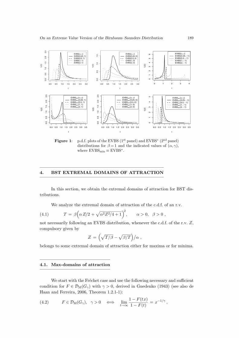
Figure 1 (first and second panels) displays shapes for the EVBS and EVBS∗

densities for different values of their parameters. In all of these graphs, we con-

sider β = 1, without loss of generality, because β is a scale parameter, such

as stated in Proposition 3.1(i). In these plots, we further use the notation

EVBS(α, γ) ≡ EVBS(α, 1, γ). For the EVBS densities presented in Figure 1 (first

panel), we see how the shape parameter α modifies the shape of these densities.

In the case of the parameter γ, we detect changes in the kurtosis, as expected.

Similar aspects are observed when we consider the EVBS∗ densities presented in

Figure 1 (second panel).


0.0 0.5 1.0 1.5 2.0 2.5 3.0

0.0

0.5

1.0

1.5

2.0

2.5

t

f Tt

EVBS

EVBS 0.25 1

EVBS 0.5 1

EVBS 1 1

EVBS 2 1

0.0 0.5 1.0 1.5 2.0 2.5 3.0

0.0

0.5

1.0

1.5

t

f Tt

EVBS

EVBS 0.25 0

EVBS 0.5 0

EVBS 1 0

EVBS 2 0

0 1 2 3 4

01

23

45

6

t

f Tt

EVBS

EVBS 0.25 1

EVBS 0.5 1

EVBS 1 1

EVBS 2 1

0.0 0.5 1.0 1.5 2.0 2.5 3.0 3.5

0.0

0.5

1.0

1.5

2.0

2.5

t

f Tt

EVBSmin

EVBSmin 0.25 1

EVBSmin 0.5 1

EVBSmin 1 1

EVBSmin 2 1

0.0 0.5 1.0 1.5 2.0 2.5 3.0 3.5

0.0

0.5

1.0

1.5

2.0

2.5

t

f Tt

EVBSmin

EVBSmin 0.25 0

EVBSmin 0.5 0

EVBSmin 1 0

EVBSmin 2 0

0.0 0.5 1.0 1.5 2.0 2.5 3.0 3.5

01

23

45

t

f Tt

EVBSmin

EVBSmin 0.25 1

EVBSmin 0.5 1

EVBSmin 1 1

EVBSmin 2 1

Figure 1: p.d.f. plots of the EVBS (1st panel) and EVBS∗ (2nd panel)distributions for β = 1 and the indicated values of (α, γ),where EVBSmin ≡ EVBS∗.

4. BST EXTREMAL DOMAINS OF ATTRACTION

In this section, we obtain the extremal domains of attraction for BST dis-

tributions.

We analyze the extremal domain of attraction of the c.d.f. of an r.v.

T = β(α Z/2 +

√α2Z2/4 + 1

)2, α > 0, β > 0 ,(4.1)

not necessarily following an EVBS distribution, whenever the c.d.f. of the r.v. Z,

compulsory given by

Z =(√

T/β −√

β/T)/

α ,

belongs to some extremal domain of attraction either for maxima or for minima.

4.1. Max-domains of attraction

We start with the Frechet case and use the following necessary and sufficient

condition for F ∈ DM(Gγ) with γ > 0, derived in Gnedenko (1943) (see also de

Haan and Ferreira, 2006, Theorem 1.2.1-1):

F ∈ DM(Gγ), γ > 0 ⇐⇒ limt→∞

1 − F (tx)

1 − F (t)= x−1/γ ,(4.2)


for all x > 0, and the right endpoint of F , namely xF := inf{x : F (x) ≥ 1}, is

necessarily infinite.

Theorem 4.1. Let the c.d.f. of the r.v. Z be in the Frechet max-domain

of attraction, necessarily with a positive EV index, i.e., γZ

> 0. Then, the c.d.f. of

the r.v. T given in (4.1) is also in the Frechet max-domain of attraction, i.e.,

FT∈ DM(Gγ

T), with γ

T= 2 γ

Z.

Proof: By hypothesis, FZ∈ DM(Gγ

Z) for γ

Z> 0. Thus, F

Zsatisfies (4.2)

for γZ. Then, we have that, as t → ∞,

1 − FT(tx)

1 − FT(t)

=1 − F

Z(atx)

1 − FZ(at)

≈ 1 − FZ

({tx/β}1/2/α

)

1 − FZ

({t/β}1/2/α

) ≈ x−1/(2γZ

) ,

with the notation ut ≈ vt being valid if and only if ut/vt → 1, as t → ∞.

For light right-tails, i.e., for the Weibull max-domain of attraction, we can

prove a result similar to that of Theorem 4.1, if we use the following necessary

and sufficient condition for F ∈ DM(Gγ) with γ < 0 (also derived in Gnedenko,

1943):

F ∈ DM(Gγ), γ < 0 ⇐⇒ limt→∞

1 − F(xF −1/{tx}

)

1 − F (xF −1/t)= x1/γ ,(4.3)

for all x > 0, and the right endpoint of F , namely xF, is finite.

Theorem 4.2. Let the c.d.f. of the r.v. Z be in the Weibull max-domain

of attraction, necessarily with a negative EV index, i.e., γZ

< 0. Then, the c.d.f. of

the r.v. T given in (4.1) is also in the Weibull max-domain of attraction and

γT

= γZ.

Proof: We have

limt→∞

1 − FT

(tF −1/{tx}

)

1−FT(tF −1/t)

= limt→∞

1 − FZ(atF−1/{tx})

1 − FZ(atF−1/t)

,

with tF being the right endpoint of FT. But we can assume, without loss of

generality, that zF, the right endpoint of FZ, is null, i.e., zF = 0. Hence, tF = β

and, as t → ∞,

1 − FZ

(atF−1/{tx}

)

1 − FZ(atF−1/t)

≈ 1 − FZ

(−{αβ tx}−1

)

1 − FZ

(−{αβ t}−1

) ≈ x1/γZ .


We next work on the slight more restrictive class of twice-differentiable

c.d.f.’s F ∈DM(Gγ), the so-called twice-differentiable domain of attraction of Gγ ,

denoted by DM(Gγ). A possible characterization of the twice-differentiable do-

main of attraction of Gγ is due to Pickands (1986). Let us then assume that there

exists F ′′, f = F ′, and consider the function

k(x) = −f(x)/{

F (x) log(F (x)

)}={− log

(− log F (x)

)}′.

Hence, with γ(x) = {1/k(x)}′, we have

(4.4) F ∈ DM(Gγ) ⇐⇒ limx↑xF

γ(x) = γ .

Consequently, if xF = +∞, limx→∞ xk(x) = 1/γ, and if xF < +∞, limx↑xF

(xF− x) k(x) = −1/γ, i.e., limx→∞ k(x) = 0, if γ > 0, and limx↑xF k(x) = +∞,

if γ < 0. If γ = 0, we can have k(x)→ 0, k(x)→+∞, or k(x)→ c, for 0 < c < +∞.

Observe also that, after some simple calculations, we can write

(4.5) γ(x) = F ′′(x)F (x) log(F (x)

)/f2(x) − log

(F (x)

)− 1 .

Theorem 4.3. Let T ∼ BST(α, β; fZ), with Z in the subset of the max-

domain of attraction of GγZ

constituted by twice-differentiable c.d.f.’s, the so-

called twice-differentiable max-domain of attraction of GγZ, and assume that

c = limt↑tF

FZ(at) log

(F

Z(at)

)A′

t

/{A2

t fZ(at)

}

is finite, where tF is the right endpoint of the r.v. T and at and At are as given

in (2.3), with A′t = dAt/dt. Then, F

T∈ DM(Gγ

T), with γ

T= γ

Z+ c.

Proof: By hypothesis, the necessary and sufficient condition (4.4) holds

for Z, with F, γ and γ(x) replaced by FZ, γ

Zand γ

Z(x), respectively. Now,

just observe that, by applying (4.5), and then (2.3)–(2.5) and A′t = −

(√t/β +

3√

β/t)/

(4αt2), we have

γT(t) =

F ′′T(t)F

T(t) log

(F

T(t))

f2T(t)

− log(F

T(t))− 1

(4.6)

=F

Z(at) log

(F

Z(at)

)A′

t

A2t f

Z(at)

+F ′′

Z(at)FZ

(at) log(F

Z(at)

)

f2Z

(at)− log

(F

Z(at)

)− 1 .

On the basis of the limit in Theorem 4.3, the first term in the second line of (4.6)

approaches c as t ↑ tF . Because the following term approaches γZ, the result

follows.

Corollary 4.1. Under the conditions of Theorem 4.3, we have c = γZ

if

γZ

> 0 and c = 0 if γZ

< 0.


Example 4.1. We now provide a few illustrations of Corollary 4.1:

(i) If Z has Frechet or Pareto distributions (in the Frechet max-domain

of attraction, i.e., γZ

> 0), then the limit in Theorem 4.3 is c = γZ

and

so γT

= 2 γZ. Indeed, as stated in Theorem 4.1, this result holds more

generally in DM(GγZ), with γ

Z> 0.

(ii) If Z has Weibull or uniform distributions (in the Weibull max-domain

of attraction, i.e., γZ

< 0), then c = 0 and γT

= γZ. In fact, as stated

in Theorem 4.2, this result holds more generally in DM(GγZ), with

γZ

< 0.

Remark 4.1. We further conjecture that, in Corollary 4.1, we can often

replace γZ

< 0 by γZ≤ 0. This is supported by the examples of an r.v. Z either

exponential or gamma, or Gumbel or normal, all in DM(G0), i.e., with γZ

= 0.

Then c = 0 and γT

= γZ

= 0. Also, if Z has an exponential-type (ET) distribution,

with a finite right endpoint, i.e., FZ(x) = K exp

(−c/{zF−x}

), for x < zF, c > 0,

and K > 0 (again in the Gumbel max-domain of attraction), then also c = 0 and

γT

= γZ

= 0.

Because in the twice-differentiable domain of attraction of Gγ the von

Mises condition is necessary and sufficient to have limx↑xF γ(x) = γ, with γ(x) =

{1/k(x)}′ (see Pickands, 1986, Theorem 5.2), we can also state that

(4.7) F ∈ DM(Gγ) ⇐⇒ limx↑xF

{1−F (x)

}F ′′(x)

/{F ′(x)

}2= −γ − 1 .

Therefore, we can still write the following result.

Theorem 4.4. Under the conditions and notations of Theorem 4.3, let

us assume that

c∗ = limt↑tF

{1−F

Z(at)

}A′

t

/{A2

t F ′Z(at)

}< ∞ .

Then, FT∈ DM(Gγ

T), with γ

T= γ

Z− c∗.

Proof: Just observe that{1−F

T(t)}

F ′′T(t)

{F ′

T(t)}2 =

{1−F

Z(at)

}{A′

tF′

Z(at) + A2

t F ′′Z

(at)}

A2t

{F ′

Z(at)

}2(4.8)

=

{1−F

Z(at)

}A′

t

A2t F ′

Z(at)

+

{1−F

Z(at)

}F ′′

Z(at){

F ′Z(at)

}2 .

By hypothesis, as t ↑ tF , the last term in (4.8) converges to −γZ− 1, and the

result follows.

Corollary 4.2. Under the conditions and notations of Theorem 4.4, if we

further assume that Z has an infinite right endpoint, then FT∈ DM(Gγ

T), with

γT

= γZ, provided there exists a finite limit for {1−F

Z(x)}/F ′

Z(x), as x → ∞.


4.2. Min-domains of attraction

We now analyze the domains of attraction for minima. To emphasize the

possible difference between the right and left EV indices, we denote this last one

as γ∗.

We reformulate conditions (4.2) and (4.3) for minima obtaining respectively

F ∈ Dm(G∗γ∗), γ∗ > 0 ⇐⇒ lim

t→−∞

F (tx)

F (t)= x−1/γ∗

, ∀x > 0 ,(4.9)

and

F ∈ Dm(G∗γ∗), γ∗< 0 ⇐⇒ lim

t→−∞

F(x

F−1/{tx}

)

F(x

F−1/t

) = x1/γ∗

, ∀x > 0 ,(4.10)

where the left endpoint xF

:= inf{x : F (x) > 0} is finite; see, e.g., Galambos (1987,

Theorem 2.1.5). Observe that a BST r.v. T cannot be in the Frechet min-domain

of attraction because its left endpoint is not −∞; see, e.g., Galambos (1987,

Theorem 2.1.4).

In the sequel, the notations Weibullmin, Frechetmin and Gumbelmin are used

for denoting Weibull, Frechet and Gumbel distributions for minima, respectively,

with parameter γ∗, and zF

and tF

denoting the left endpoints of Z and T , respec-

tively.

Theorem 4.5. Let the c.d.f. of the r.v. Z be in the Weibull min-domain

of attraction, necessarily with a negative EV index, i.e., γ∗Z

< 0. Then, the c.d.f. of

the r.v. T given in (4.1) is in the Weibull min-domain of attraction and γ∗T

= γ∗Z.

Proof: Assume, without loss of generality, that zF

= 0, with zF

being the

left endpoint of FZ

(i.e., tF

= β, with tF

being the left endpoint of FT). Then,

limt→−∞

FT

(tF−1/{tx}

)

FT

(tF−1/t

) = limt→−∞

FZ

(at

F−1/{tx}

)

FZ

(at

F−1/t

) = limt→−∞

FZ

(−{αβ tx}−1

)

FZ

(−{αβ t}−1

)

and the result follows from the fact that FZ

satisfies (4.10) for γ∗Z.

Theorem 4.6. Let the c.d.f. of the r.v. Z be in the Frechet min-domain of

attraction, necessarily with a positive EV index, i.e., γ∗Z

> 0. Then, the c.d.f. of the

r.v. T given in (4.1) is in the Weibull min-domain of attraction, and γ∗T

= −2 γ∗Z.

Proof: Consider, without loss of generality, tF

= 0. Then, zF

= −∞ and

limt→−∞

FT

(tF−1/{tx}

)

FT

(tF−1/t

) = limt→−∞

FZ

(a−1/{tx}

)

FZ

(a−1/t

)

= limt→−∞

FZ

(−{−β tx}1/2/α

)

FZ

(−{−β t}1/2/α

) = x−1/(2γ∗

Z) ,

where the last step is due to the fact that FZ

satisfies (4.9) for γ∗Z.


Next, we again work on the slight more restrictive class of twice-differentiable

c.d.f.’s, such as in Subsection 4.1. Analogously to the domain of attraction for

maxima, the von Mises condition in (4.7), reformulated for minima, enables us

to state that

F ∈ Dm(G∗γ∗) ⇐⇒ lim

x↓xF

F (x)F ′′(x)/(F ′(x)

)2= γ∗ + 1 ,(4.11)

where xF

is the left endpoint of F and Dm(G∗γ∗) denotes the twice-differentiable

domain of attraction of G∗γ∗ .

Theorem 4.7. Let T ∼ BST(α, β; fZ), with Z in the subset of the min-

domain of attraction of G∗γ∗

Z

constituted by the twice-differentiable c.d.f.’s, the

so-called twice-differentiable min-domain of attraction of G∗γ∗

Z

, and assume that

d = limt↓t

F

FZ(at)A

′t

/(A2

t F ′Z(at)

)

is finite, where tF

is the left endpoint of T and at and At are as given in (2.3),

with A′t = dAt/dt. Then, F

T∈ D∗

m(G∗γ∗

T

), with γ∗T

= γ∗Z

+ d.

Proof: The result is easy to prove because

FT(t)F ′′

T(t)

fT(t)2

=F

Z(at)

{A′

tfZ(at) + A2

t F ′′Z

(at)}

A2t f

Z(at)2

=F

Z(at)A

′t

A2t f

Z(at)

+F

Z(at)F

′′Z

(at)

fZ(at)2

.

Corollary 4.3. Under the conditions of Theorem 4.7, we have d = 0 if

γ∗Z

< 0 and d = −3 γ∗Z

if γ∗Z

> 0.

Example 4.2. We next provide a few illustrations of Corollary 4.3:

(i) If Z has a Weibull distribution for minima (in the Weibull min-

domain of attraction, i.e., γ∗Z

< 0), or an exponential, Pareto or uni-

form distribution (also in the Weibull min-domain of attraction, with

γ∗Z

= −1), or even a Gamma(p, q) distribution (in the Weibull min-

domain of attraction, with γ∗Z

= −1/p), then d = 0 and γ∗T

= γ∗Z.

Indeed, as stated in Theorem 4.5, this result holds more generally

in Dm(G∗γ∗

Z

), with γ∗Z

< 0.

(ii) If Z has a Frechet distribution for minima (in the Frechet min-domain

of attraction, i.e., γ∗Z

> 0), then d = −3 γ∗Z

and γ∗T

= −2 γ∗Z. In fact, as

stated in Theorem 4.6, this result holds more generally in Dm(G∗γ∗

Z

),

with γ∗Z

> 0.

(iii) If Z has an ET distribution as in Remark 4.1 (in the Frechet min-

domain of attraction, with γ∗Z

= 1), then d = −3 γ∗Z

=−3 and γ∗T

= −2,

i.e., T belongs to the Weibull min-domain of attraction.


Remark 4.2. Similarly to what we mentioned in Remark 4.1, we further

conjecture that, in Corollary 4.3, we can often replace γ∗Z

< 0 by γ∗Z≤ 0. This is

supported by the fact that if Z has a Gumbel distribution for minima, or any of

the limiting distributions for maxima (Frechet, Gumbel, Weibull), or a normal

distribution (all in the Gumbel min-domain of attraction, i.e. γ∗Z

= 0), then the

limit in Theorem 4.7 is d = 0 and γ∗T

= γ∗Z

= 0.

5. HAZARD ANALYSIS

We may define a hazard as a dangerous event that could conduct to an emer-

gency or disaster. The origin of this event may be due to a situation that could

have an adverse effect. Thus, a hazard is a potential and not an actual possibility,

i.e., it can be statistically evaluated. A hazard analysis is the assessment of a risk

that is present in a particular environment. Therefore, hazard assessment allows

us to evaluate potential risk by the estimated frequency or intensity of the r.v. of

interest. In this section, we study the EVBS h.r. and its change point.

5.1. Hazard rate

Statistically, a hazard analysis can be carried out by the h.r. function.

Apart from hazard rate, this function is also known as chance function, fail-

ure rate, force of mortality, intensity function, or risk rate, among other names.

In actuarial science, for example, the h.r. is the annualized probability that a

person at a specified age will die in the next instant, expressed as a death rate

per year. For more details about the concept of h.r., see Marshall and Olkin

(2007, pp. 10–13).

A nice property of the h.r. is that it allows us to characterize the behavior of

statistical distributions. For example, the h.r. may have several different shapes

such as increasing (IHR), constant (exponential distribution), decreasing (DHR),

bathtube (BT), inverse bathtube (IBT or upside-down) approaching to a non-

null constant and IBT approaching to zero. An incorrect specification of the

h.r. could have serious consequences in the analysis; see, e.g., Bhatti (2010) for a

study about this issue.

The h.r. of an r.v. T is given in general by hT(t) = f

T(t)/R

T(t), for t > 0,

and 0 < FT(t) < 1, where R

T(t) = 1 − F

T(t), for t > 0, is the reliability function

(r.f.), and fT

and FT

are the p.d.f. and c.d.f. of the r.v. T . The change point

of hT(t), denoted by tc, is defined as the moment where the h.r. attains either

a maximum or a minimum value and it is the solution of the equation f(tc) =

−f ′(tc)/h(tc), whenever F is twice-differentiable, and such a solution exists.


5.2. TTT curve

The h.r. of an r.v. T can be characterized by its corresponding total time

on test (TTT) function given by

H−1T

(u) =

∫ F−1

T(u)

0

(1 − F

T(y))dy

or by its scaled version given by WT(u) = H−1

T(u)/H−1

T(1), for 0 ≤ u ≤ 1, where

once again F−1T

is the generalized inverse function of the c.d.f. of T . Now,

WT

can be empirically approximated, allowing to construct the empirical scaled

TTT curve by plotting the consecutive points[k/n, Wn(k/n)

], where Wn(k/n) ={∑k

i=1 T(i) + (n− k)T(k)

}/∑ni=1 T(i), for k = 1, ..., n, with T(i) being the corre-

sponding ith ascending order statistic, for 1 ≤ i ≤ n.

From Figure 2 (left), we observe different theoretical shapes for the scaled

TTT curve. Thus, a TTT plot expressed by a curve that is concave (or con-

vex) corresponds to the IHR (or DHR) class. A concave (or convex) and then

convex (or concave) shape for the TTT curve corresponds to a IBT (or BT) h.r.

A TTT plot represented by a straight line is an indication that the exponential

distribution must be used. Thus, a graphical plot of the empirical scaled TTT

curve could provide to us the type of distribution that the data have. See also in

Figure 2 the theoretical scaled TTT curves for EVBS (center) and EVBS∗ (right)

models. In these plots, we again use the notation EVBS(α, γ) ≡ EVBS(α, 1, γ).

WT (

u)

1.0

1.00.0u

incr

easi

ng

decreasing

cons

tant

bath

tub

inverse bathtub

!"! !"# !"$ !"% !"& '"!

!"!

!"#

!"$

!"%

!"&

'"!

(

)*!("

+,-.!#$%&"+,-.!' #$%'/ $"+,-.!' #$%'' $"+,-.!' #$%!"+,-.!' #$%' $"+,-.!' #$%/ $"

!"! !"# !"$ !"% !"& '"!

!"!

!"#

!"$

!"%

!"&

'"!

(

)*!("

+,-./01!#$%&"+,-./01!' #$%2 $"+,-./01!' #$%' $"+,-./01!' #$%!"+,-./01!' #$%'' $"+,-./01!' #$%'2 $"

Figure 2: Theoretical scaled TTT curves for a general distribution with theindicated h.r. shape (left) and for the EVBS(0.5, γ) (center) andEVBS∗(0.5, γ) (right) distributions for the indicated values of γ.


5.3. EVBS hazard rate

The normal distribution is in the IHR class. The gamma and Weibull

distributions can be either in IHR or DHR classes (of course, the case of the

exponential distribution with constant h.r. is considered by these two models).

However, the lognormal (LN) distribution has a non-monotonic h.r., because it

is initially increasing until its change point and then it decreases to zero, i.e.,

the LN model is in the IBT h.r. class. The BS h.r. behaves similarly to the LN

h.r., i.e., it is initially increasing until its change point and then decreasing not

to zero, but to a positive constant. Thus, although BS, gamma, LN and Weibull

distributions have densities with similar shapes, their h.r.’s are totally different.

Let T ∼ EVBS(α, β, γ). Then, directly from the definition of the p.d.f.,

fT(t), and the c.d.f., F

T(t), of the r.v. T ∼ EVBS(α, β, γ), given in (3.2) and

(3.3), respectively, we have that:

A. The r.f. of T is expressed as RT(t) = 1−F

T(t), with F

T(t) given in (3.3).

B. Again with at and At as given in (2.3), the h.r. of T is defined as

hT(t) =

fT(t)

RT(t)

=

{At(1+ γat)

−1−1/γ/(

exp({1+ γat}−1/γ

)−1); γ 6= 0 ,

At exp(−at)/exp(exp(−at)

)−1; γ = 0 ,

where t > (α2β + 2βγ2)/(2 γ2) −√

(α4β2 + 4α2β2γ2)/γ4/2 if γ > 0;

t>0 if γ=0; and 0<t<(α2β + 2βγ2)/(2γ2)+√

(α4β2 +4α2β2γ2)/γ4/2

if γ < 0.

C. With the notation btc = 1 + γatc , the change point tc of the h.r. of T

is obtained as the solution of the equations:

({A′

tc−A2tc(1 + γ)b−1

tc

}{exp(b−1/γtc

)− 1}

+

+ A2tc

{1 + γatc

}−1−1/γexp(b−1/γtc

))b−1−1/γtc = 0 ; γ 6= 0 ,

A2tc

(1 +

{exp(−atc)− 1

}exp(exp(−atc)

))+

+ A′tc

(exp(exp(−atc)

)− 1)

= 0 ; γ = 0 .

Let T ∗ ∼ EVBS∗(α, β, γ). Then, now, directly from the definition of the

p.d.f., fT∗

(t), and the c.d.f., FT∗

(t), of the r.v. T ∗ ∼ EVBS∗(α, β, γ), given in (3.4)

and (3.5), respectively, we have that:


D. The r.f. of T ∗ is expressed as RT∗

(t) = 1−FT∗

(t), with FT∗

(t) as given

in (3.5).

E. Again with at and At as given in (2.3), the h.r. of T ∗ is defined as

hT∗

(t) =f

T∗(t)

RT∗

(t)=

{At(1 − γat)

−1−1/γ ; γ 6= 0 ,

At exp(at); γ = 0 ,

where t > (α2β + 2βγ2)/(2 γ2) −√

(α4β2 + 4α2β2γ2)/γ4/2 if γ < 0;

t>0 if γ=0; and 0<t<(α2β + 2βγ2)/(2γ2) +√

(α4β2 +4α2β2γ2)/γ4/2

if γ > 0.

F. The change point tc of the h.r. of T ∗ is obtained as the solution of the

equations:

{(1 − γatc)

−1−1/γ(A′

tc + {1 + γ}A2tc{1− γatc}−1

)= 0; γ 6= 0 ,

A2tc + A′

tc = 0; γ = 0 .

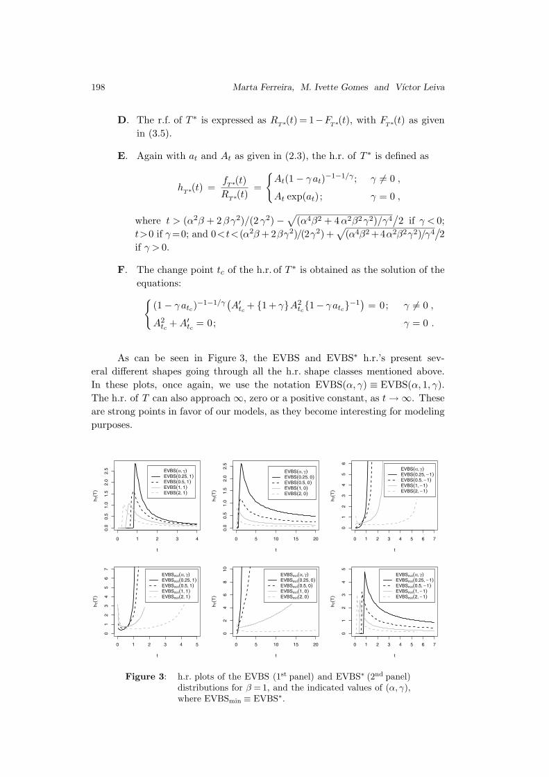
As can be seen in Figure 3, the EVBS and EVBS∗ h.r.’s present sev-

eral different shapes going through all the h.r. shape classes mentioned above.

In these plots, once again, we use the notation EVBS(α, γ) ≡ EVBS(α, 1, γ).

The h.r. of T can also approach ∞, zero or a positive constant, as t → ∞. These

are strong points in favor of our models, as they become interesting for modeling

purposes.

0 1 2 3 4

0.0

0.5

1.0

1.5

2.0

2.5

t

hT

T

EVBS

EVBS 0.25 1

EVBS 0.5 1

EVBS 1 1

EVBS 2 1

0 5 10 15 20

0.0

0.5

1.0

1.5

2.0

2.5

t

hT

T

EVBS

EVBS 0.25 0

EVBS 0.5 0

EVBS 1 0

EVBS 2 0

0 1 2 3 4 5 6 7

01

23

45

6

t

hT

T

EVBS

EVBS 0.25 1

EVBS 0.5 1

EVBS 1 1

EVBS 2 1

0 1 2 3 4 5

01

23

45

67

t

hT

T

EVBSmin

EVBSmin 0.25 1

EVBSmin 0.5 1

EVBSmin 1 1

EVBSmin 2 1

0 5 10 15 20

02

46

810

t

hT

T

EVBSmin

EVBSmin 0.25 0

EVBSmin 0.5 0

EVBSmin 1 0

EVBSmin 2 0

0 1 2 3 4 5 6 7

01

23

45

t

hT

T

EVBSmin

EVBSmin 0.25 1

EVBSmin 0.5 1

EVBSmin 1 1

EVBSmin 2 1

Figure 3: h.r. plots of the EVBS (1st panel) and EVBS∗ (2nd panel)distributions for β = 1, and the indicated values of (α, γ),where EVBSmin ≡ EVBS∗.


6. ESTIMATION AND MODEL CHECKING

In this section, we present some results related to estimation aspects and

model checking for EVBS distributions.

6.1. ML estimation

As is well-known, ML estimates are obtained from the solution of the system

ℓ(θ) ≡ 0, where ℓ(θ) denotes the score vector of first derivatives of the logarithm

of the likelihood function for θ, namely ℓ(θ). In our case, if we consider the EVBS

model (the procedure is similar for the EVBS∗ model), this function is given by

ℓ(θ) =∑n

i=1 ℓi(θ), where, for i = 1, ..., n,

ℓi(θ) =

{log(Ati) −

(1 + 1

γ

)log(1 + γati) − (1 + γati)

−1/γ ; γ 6= 0 ,

log(Ati) − exp(−ati) − ati ; γ = 0 ,

with θ = [α, β, γ]⊤. The score vector ℓ(θ) = ∂ℓ(θ)/∂θ = [ℓθ1], with θ1 = α, β, or γ,

is given by

−n

α+

n∑

i=1

( {1+ γ}ati

α{1+ γati} − 1

αati

{1+ γati}−1−1/γ

)

n∑

i=1

−

α

2β

ati√ti

β +√

βti

+{1+ γ}

2αβ {1+γati}

{√tiβ

+

√β

ti

}−

√ti

β +√

βti

2αβ{1+ γati

}−1−1/γ

n∑

i=1

(−{1+ γati

}−1/γ

γ2

{log(1+ γati

) − γati

1+ γati

}− {γ +1}ati

γ{1+ γati} +

log(1+ γati)

γ2

)

,

whenever γ 6= 0 and, if γ = 0, is given by

−n

α−

n∑

i=1

(1

αexp(−ati

)ati− 1

αati

)

n∑

i=1

(− 1

2αβexp(−ati

)

{√tiβ

+

√β

ti

}+

1

2αβ

{√tiβ

+

√β

ti

}− α

2β

ati√ti/β +

√β/ti

)

.

In this case, the system of likelihood equations ℓ(θ) ≡ 0 does not produce an expli-

cit solution so that a numerical procedure is necessary. To this end, initial values

for the parameters α, β and γ can be obtained using the methods to be described

in Subsection 6.2. In addition, these likelihood equations seem to be often unstable.


We propose to use the following approach for solving this problem of instability.

The approach consists of obtaining the optimum value for the parameter γ assum-

ing it to be known, for example, following a similar algorithm to that proposed by

Rinne (2009, pp. 426–433) and called by him as non-failing (NF); see also Barros

et al. (2009) and Leiva et al. (2011). In these works, they fixed values for their

parameter, in our case γ, within a set of several possible values for this parameter,

and they then estimate the structural parameters, in our case, α and β. Finally,

we consider the fixed γ that maximizes the likelihood function. Specifically, this

approach is based on a partition of the real number set into a suitable amount of

sub-intervals. Fixing γ in each of these intervals, we estimate α and β by using

the ML method and then we look for the value of γ that maximizes the likelihood

function. In this case, the NF algorithm is given by:

NF1 For a fixed value of γ:

NF1.1 Estimate the parameters α and β of the EVBS model using

the estimates of α and β from the procedure to be described

in Subsection 6.2 as starting values.

NF1.2 Compute the associated likelihood function.

NF2 Choose the value of γ that maximizes the likelihood function and

then consider the obtained ML estimates of α and β as result.

6.2. Starting estimation

Firstly, to find initial values for the numerical optimization procedure

needed for the ML estimation of the EVBS distribution parameters described

in Subsection 6.1, we introduce a graphical method analogous to the probability

plots; see Leiva et al. (2008a). This method is useful for goodness-of-fit and can

also be used as an estimation method or, at least, to find initial values for an

iterative procedure. The method consists of transforming the data forming pairs

of values that should follow a linear relationship if these data would come from

the EVBS distribution. Then, by using a simple linear regression method, the

slope and intercept of this linear relationship are estimated. The line is used

for goodness-of-fit such as a quantile versus quantile (QQ) plot. Specifically,

if we consider the EVBS c.d.f. as given in (2.2), but with Φ replaced by FZ,

we have t = β + α√

β√

t F−1Z

(FT(t)), where F−1

Zis the generalized inverse c.d.f.

of the generator EV distribution and FT

is the EVBS c.d.f. However, it is difficult

to derive a linear function over t in the above expression, which is fundamental for

probability plots. We consider p =√

t F−1Z

(FT(t)) obtaining the linear function

y ≈ a + b x, where x = p, y = t, the intercept is a = β, and the slope is b = α√

β.

Now, suppose we have n ordered observations, say t(1) ≤ ... ≤ t(n). Because we


can estimate FT(t(i)) by qi = (i − 0.3)/(n + 0.4), for i = 1, ..., n, the graphical

plot of t(i) versus pi, where pi =√

t(i) F−1Z

(qi) is approximately a straight line

whenever the data come from some EVBS distribution. Goodness-of-fit can be

visually and analytically studied using the coefficient of determination of the fit

of regression between t(i) and pi. Therefore, the parameters α and β of this dis-

tribution can be estimated by using the least square method obtaining β = a and

α = b/√

a.

Secondly, to find an initial value for the parameter γ, we can use a landmark

from the EV theory. This landmark is the result about the limiting generalized

Pareto (GP) behavior of the scaled excesses; see, e.g., Balkema and de Haan

(1974) and Pickands (1975). This enables the development of the so-called ML

EV index estimators, which we can take as an initial value for γ to be used

for the numerical optimization procedure needed for the ML estimation of the

EVBS distribution parameters. We refer the peaks over threshold methodology

of estimation (see Smith, 1987) as well as the methodology used by Drees et al.

(2004), named peaks over random threshold in Araujo Santos et al. (2006).

6.3. Model checking

Once the EVBS distribution parameters are estimated, a natural ques-

tion that arises is checking how good is the fit of the model to the data. We

can use the invariance property of the ML estimators for fitting the p.d.f. and

c.d.f. of the EVBS model. Also, to compare the EVBS distributions to other

distributions, we can use model selection procedure based on loss of information,

such as Akaike (AIC), Schwarz’s Bayesian (BIC) and Hannan–Quinn (HQIC)

information criteria. These criteria allow us to compare models for the same

data set and are given by AIC = −2 ℓ(θ) + 2d, BIC = −2 ℓ(θ) + d log(n), and

HQIC = −2 ℓ(θ) + 2 d log(log(n)), where, as mentioned, ℓ(θ) is the log-likelihood

function for the parameter θ associated with the model evaluated at θ = θ, n is

the sample size, and d is the dimension of the parameter space.

AIC, BIC and HQIC are based on a penalization of the likelihood function

as the model becomes more complex, i.e., with more parameters. Thus, a model

whose information criterion has a smaller value is better. This is an important

point, because the EVBS distribution has more parameters than the usual BS

distribution. Because models with more parameters always provide a better fit,

AIB, BIC and HQIC allow us to compare models with different numbers of pa-

rameters due to the penalization incorporated in such criteria. This methodology

is very general and can be applied even to non-nested models, i.e., those models

that are not particular cases of a more general model; see Vilca et al. (2011) and

references therein.


Generally, differences between two values of the information criteria are not

very noticeable. In that case, the Bayes factor (BF) can be used to highlight such

differences, if they exist. To define the BF, assume the data D belong to one of

two hypothetical models, namely M1 and M2, according to probabilities P(D|M1)

and P(D|M2), respectively. Given probabilities P(M1) and P(M2) = 1 − P(M1),

the data produce conditional probabilities P(M1|D) and P(M2|D) = 1−P(M1|D),

respectively. Then, the BF that allow us to compare M1 (model considered as

correct) to M2 (model to be contrasted with M1) is given by

B12 =P(D|M1)

P(D|M2).(6.1)

Based on (6.1), we can use the approximation

(6.2) 2 log(B12) ≈ 2[ℓ(θ1) − ℓ(θ2)

]−[d1 − d2

]log(n) ,

where ℓ(θk) is the log-likelihood function for the parameter θk under the model

Mk evaluated at θk = θk, dk is the dimension of θk, for k = 1, 2, and n is the

sample size. Notice that the approximation in (6.2) is computed subtracting the

BIC value from the model M2, given by BIC2 = −2 ℓ(θ2) + d2 log(n), to the BIC

value of the model M1, given by BIC1 = −2 ℓ(θ1) + d1 log(n). In addition, notice

that if model M2 is a particular case of M1, then the procedure corresponds to ap-

plying the likelihood ratio (LR) test. In this case, 2 log(B12) ≈ χ212 − df12 log(n),

where χ212 is the LR test statistic for testing M1 versus M2 and df12 = d1− d2 are

the d.f.’s associated with the LR test, so that one can obtain the corresponding

p-value from 2 log(B12)·∼ χ2(d1 − d2), with d1 > d2.

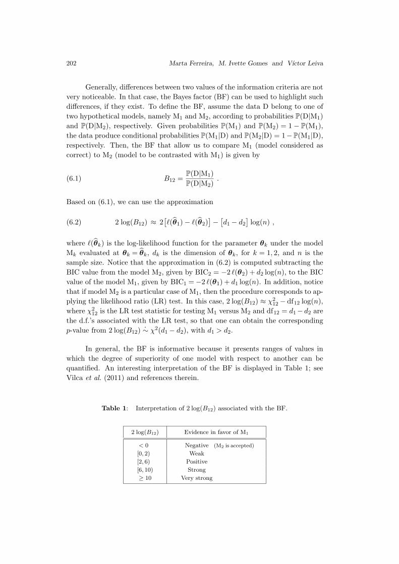
In general, the BF is informative because it presents ranges of values in

which the degree of superiority of one model with respect to another can be

quantified. An interesting interpretation of the BF is displayed in Table 1; see

Vilca et al. (2011) and references therein.

Table 1: Interpretation of 2 log(B12) associated with the BF.

2 log(B12) Evidence in favor of M1

< 0 Negative (M2 is accepted)

[0, 2) Weak

[2, 6) Positive

[6, 10) Strong

≥ 10 Very strong


7. APPLICATION

In this section, to illustrate some of the results obtained in this study, we fit

the EVBS∗ model (for minimum) to a real data set corresponding to air pollutant

concentrations. We assume that the data are uncorrelated and independent and,

therefore, a diurnal or cyclic trend analysis is not necessary. This assumption has

been supported by some authors for different reasons; see, e.g., Vilca et al. (2010)

and references therein. For example, environmental data are sometimes reported

as average or total values and so spatiotemporal dependence is missing. In this

analysis, we first discuss an implementation in R code of the EVBS model. Next,

the data set upon analysis is introduced. Then, an EDA is produced. Finally,

estimation and EVBS model checking are carried out.

7.1. Implementation in R code

Several R packages for analyzing data from different distributions are avail-

able from CRAN (for example, the bs and gbs packages). An R package named

evbs to analyze data from EVBS models is being developed by the authors, whose

“in progress” version is available upon request. This package contains diverse in-

dicators and methodologies useful for EVBS distributions. In addition, the evbs

package incorporates the scaled TTT curve as a descriptive tool to identify the

possible shape of the h.r.

7.2. The data set

The data correspond to daily ozone concentrations that were collected in

New York during May–September, 1973. These data were taken from Nadarajah

(2008) and have been provided by the New York State Department of Conserva-

tion. This set of daily ozone level measurements (in ppb = ppm×1000), that we

call from now simply ozone, are: 41, 36, 12, 18, 28, 23, 19, 8, 7, 16, 11, 14, 18, 14, 34,

6, 30, 1, 11, 4, 32, 23, 45, 115, 37, 29, 71, 39, 23, 21, 37, 20, 12, 13, 49, 32, 64, 40, 77, 97,

97, 85, 10, 27, 7, 48, 35, 61, 79, 63, 16, 108, 20, 52, 82, 50, 64, 59, 39, 9, 16, 78, 35, 66,

122, 89, 110, 44, 65, 22, 59, 23, 31, 44, 21, 9, 45, 168, 73, 76, 118, 84, 85, 96, 78, 91, 47,

32, 20, 23, 21, 24, 44, 21, 28, 9, 13, 46, 18, 13, 24, 16, 23, 36, 7, 14, 30, 14, 18, 20, 11,

135, 80, 28, 73, 13.


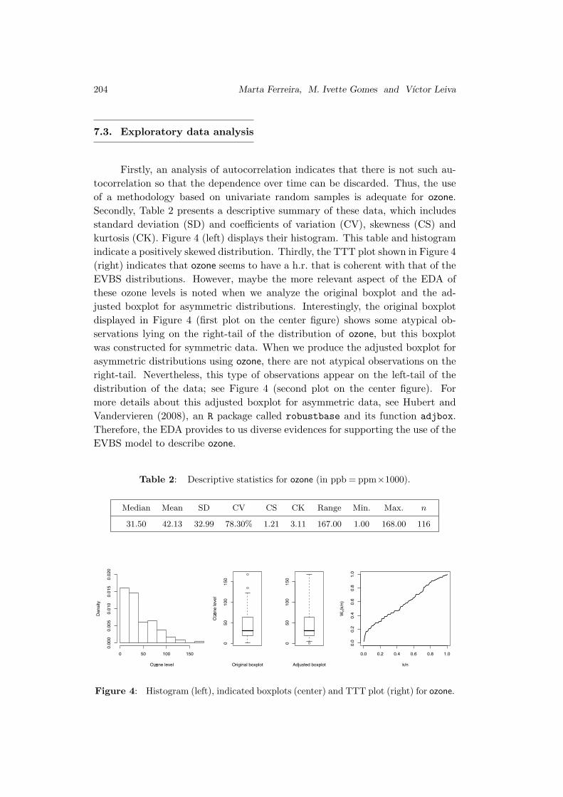
7.3. Exploratory data analysis

Firstly, an analysis of autocorrelation indicates that there is not such au-

tocorrelation so that the dependence over time can be discarded. Thus, the use

of a methodology based on univariate random samples is adequate for ozone.

Secondly, Table 2 presents a descriptive summary of these data, which includes

standard deviation (SD) and coefficients of variation (CV), skewness (CS) and

kurtosis (CK). Figure 4 (left) displays their histogram. This table and histogram

indicate a positively skewed distribution. Thirdly, the TTT plot shown in Figure 4

(right) indicates that ozone seems to have a h.r. that is coherent with that of the

EVBS distributions. However, maybe the more relevant aspect of the EDA of

these ozone levels is noted when we analyze the original boxplot and the ad-

justed boxplot for asymmetric distributions. Interestingly, the original boxplot

displayed in Figure 4 (first plot on the center figure) shows some atypical ob-

servations lying on the right-tail of the distribution of ozone, but this boxplot

was constructed for symmetric data. When we produce the adjusted boxplot for

asymmetric distributions using ozone, there are not atypical observations on the

right-tail. Nevertheless, this type of observations appear on the left-tail of the

distribution of the data; see Figure 4 (second plot on the center figure). For

more details about this adjusted boxplot for asymmetric data, see Hubert and

Vandervieren (2008), an R package called robustbase and its function adjbox.

Therefore, the EDA provides to us diverse evidences for supporting the use of the

EVBS model to describe ozone.

Table 2: Descriptive statistics for ozone (in ppb = ppm×1000).

Median Mean SD CV CS CK Range Min. Max. n

31.50 42.13 32.99 78.30% 1.21 3.11 167.00 1.00 168.00 116

Ozone level

Density

0 50 100 150

0.0

00

0.0

05

0.0

10

0.0

15

0.0

20

050

100

150

Original boxplot

Ozone level

050

100

150

Adjusted boxplot

0.0 0.2 0.4 0.6 0.8 1.0

0.0

0.2

0.4

0.6

0.8

1.0

k/n

Wn(k/n)

Figure 4: Histogram (left), indicated boxplots (center) and TTT plot (right) for ozone.


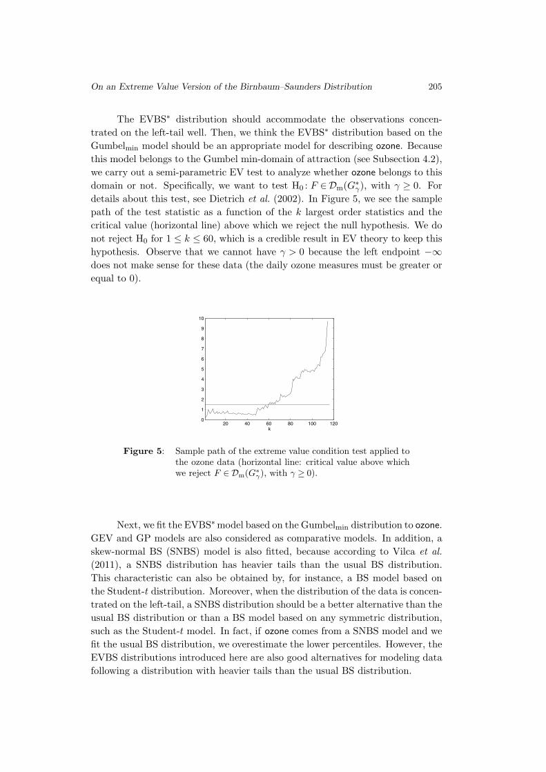
The EVBS∗ distribution should accommodate the observations concen-

trated on the left-tail well. Then, we think the EVBS∗ distribution based on the

Gumbelmin model should be an appropriate model for describing ozone. Because

this model belongs to the Gumbel min-domain of attraction (see Subsection 4.2),

we carry out a semi-parametric EV test to analyze whether ozone belongs to this

domain or not. Specifically, we want to test H0 : F ∈Dm(G∗γ), with γ ≥ 0. For

details about this test, see Dietrich et al. (2002). In Figure 5, we see the sample

path of the test statistic as a function of the k largest order statistics and the

critical value (horizontal line) above which we reject the null hypothesis. We do

not reject H0 for 1 ≤ k ≤ 60, which is a credible result in EV theory to keep this

hypothesis. Observe that we cannot have γ > 0 because the left endpoint −∞does not make sense for these data (the daily ozone measures must be greater or

equal to 0).

20 40 60 80 100 1200

1

2

3

4

5

6

7

8

9

10

k

Figure 5: Sample path of the extreme value condition test applied tothe ozone data (horizontal line: critical value above whichwe reject F ∈ Dm(G∗

γ), with γ ≥ 0).

Next, we fit the EVBS∗ model based on the Gumbelmin distribution to ozone.

GEV and GP models are also considered as comparative models. In addition, a

skew-normal BS (SNBS) model is also fitted, because according to Vilca et al.

(2011), a SNBS distribution has heavier tails than the usual BS distribution.

This characteristic can also be obtained by, for instance, a BS model based on

the Student-t distribution. Moreover, when the distribution of the data is concen-

trated on the left-tail, a SNBS distribution should be a better alternative than the

usual BS distribution or than a BS model based on any symmetric distribution,

such as the Student-t model. In fact, if ozone comes from a SNBS model and we

fit the usual BS distribution, we overestimate the lower percentiles. However, the

EVBS distributions introduced here are also good alternatives for modeling data

following a distribution with heavier tails than the usual BS distribution.


7.4. Estimation and checking model

To find the ML estimates of the EVBS distribution parameters, we use the

procedure described in Subsections 6.1 and 6.2. Thus, based on ozone, we obtain

the ML estimates along with the values of AIC, BIC, HQIC and BF used for

model selection; see Table 3.

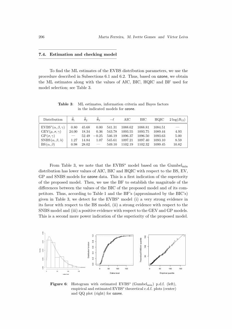
Table 3: ML estimates, information criteria and Bayes factorsin the indicated models for ozone.

Distribution bθ1 bθ2bθ3 −ℓ AIC BIC HQIC 2 log(B12)

EVBS∗(α, β, γ) 0.80 45.68 0.00 541.31 1088.62 1088.81 1084.51 —

GEV(µ, σ, γ) 24.00 18.34 0.36 543.78 1093.55 1093.75 1089.44 4.93GP(σ, γ) — 52.49 −0.25 546.19 1096.37 1096.50 1093.63 5.00SNBS(α, β, λ) 1.27 14.84 1.07 545.61 1097.21 1097.40 1093.10 8.59BS(α, β) 0.98 28.02 — 549.10 1102.19 1102.32 1099.45 10.82

From Table 3, we note that the EVBS∗ model based on the Gumbelmin

distribution has lower values of AIC, BIC and HQIC with respect to the BS, EV,

GP and SNBS models for ozone data. This is a first indication of the superiority

of the proposed model. Then, we use the BF to establish the magnitude of the

differences between the values of the BIC of the proposed model and of its com-

petitors. Thus, according to Table 1 and the BF’s (approximated by the BIC’s)

given in Table 3, we detect for the EVBS∗ model (i) a very strong evidence in

its favor with respect to the BS model, (ii) a strong evidence with respect to the

SNBS model and (iii) a positive evidence with respect to the GEV and GP models.

This is a second more power indication of the superiority of the proposed model.

ozone level

Density

0 50 100 150

0.0

00

0.0

05

0.0

10

0.0

15

0.0

20

0 50 100 150

0.0

0.2

0.4

0.6

0.8

1.0

Ozone level

Dis

trib

ution f

unction

0 50 100 150

50

100

150

Empirical quantile

Theore

tical E

VB

Sm

in q

uantile

Figure 6: Histogram with estimated EVBS∗ (Gumbelmin) p.d.f. (left),empirical and estimated EVBS∗ theoretical c.d.f. plots (center)and QQ plot (right) for ozone.


Now, from Figure 6 (center), we see the excellent coherence between the empirical

and EVBS theoretical c.d.f.’s. for ozone. Moreover, a QQ plot for the EVBS

distribution shown in Figure 6 (right) confirms such a coherence between the

EVBS∗ model and the data. In fact, the histogram and the estimated EVBS∗

p.d.f. based on the Gumbelmin distribution provided in Figure 6 (left) also shows

an excellent fit of the EVBS∗ model to these ozone data. Therefore, we conclude

that the EVBS∗ distribution provides a much better fit than the other considered

models for the ozone data analyzed in this study.

8. CONCLUDING REMARKS

This article has dealt with an extreme value version of the Birnbaum–

Saunders distribution. Specifically, we have found the density of the extreme

value Birnbaum–Saunders distribution and discussed its shape. We have obtained

the cumulative distribution and quantile functions of this distribution as well

as highlighted some of their properties. Extremal domains of attraction for

Birnbaum–Saunders type distributions have been studied. A characterization

of the hazard rate of extreme value Birnbaum–Saunders distributions has been

also carried out. We have developed an R package with the obtained results and

used part of it for analyzing a real data set of ozone concentrations. This analysis

has allowed us to show the adequacy of these new statistical distributions.

ACKNOWLEDGMENTS

Marta Ferreira was partially supported by the Research Centre of Mathe-

matics of the University of Minho through the FCT Pluriannual Funding Program

and by PTDC/FEDER grants from Portugal. M. Ivette Gomes was partially sup-

ported by national funds through FCT (Fundacao para a Ciencia e a Tecnologia)

by PEst-OE/MAT/UI0006/2011, FCT/OE, POCI 2010 and PTDC/FEDER grants

from Portugal. Vıctor Leiva was supported by FONDECYT (Fondo Nacional de

Desarrollo Cientıfico y Tecnologico) by 1120879 grant and project DIPUV 43/2010,

both from Chile.


REFERENCES

[1] Ahmed, S.E.; Castro-Kuriss, C.; Flores, E.; Leiva, V. and Sanhueza, A.

(2010). A truncated version of the Birnbaum–Saunders distribution with an appli-cation in financial risk, Pak. J. Statist., 26, 293–311.

[2] Araujo Santos, P.; Fraga Alves, M.I. and Gomes, M.I. (2006). Peaks overrandom threshold methodology for tail index and quantile estimation, Revstat, 4,227–247.

[3] Balkema, A.A. and de Haan, L. (1974). Residual life time at great age, Ann.

Probab., 2, 792–804.

[4] Barros, M.; Paula, G.A. and Leiva, V. (2008). A new class of survivalregression models with heavy-tailed errors: robustness and diagnostics, Lifetime

Data Anal., 14, 316–332.

[5] Barros, M.; Paula, G.A. and Leiva, V. (2009). An R implementation forgeneralized Birnbaum–Saunders distributions, Comp. Statist. Data Anal., 53,1511–1528.

[6] Beirlant, J.; Goegebeur, Y.; Segers, J. and Teugels, J. (2004). Statistics

of Extremes: Theory and Application, John Wiley and Sons, New York.

[7] Beirlant, J.; Caeiro, F. and Gomes, M.I. (2012). An overview and openresearch topics in statistics of univariate extremes, Revstat, 10, 1–31.

[8] Bhatti, C.R. (2010). The Birnbaum–Saunders autoregressive conditional dura-tion model, Math. Comp. Simul., 80, 2062–2078.

[9] Birnbaum, Z.W. and Saunders, S.C. (1969). A new family of life distributions,J. Appl. Probab., 6, 319–327.

[10] Coles, S. (2001). An Introduction to Statistical Modeling of Extreme Values,Springer, London.

[11] Dıaz-Garcıa, J.A. and Leiva,V. (2005). A new family of life distributions basedon elliptically contoured distributions, J. Statist. Plan. Infer., 128, 445–457(Erratum: J. Statist. Plan. Infer., 137, 1512–1513).

[12] Dietrich, D.; de Haan, L. and Husler, J. (2002). Testing extreme valueconditions, Extremes, 5, 71–85.

[13] Drees, H.; Ferreira, A. and de Haan, L. (2004). On maximum likelihoodestimation of the extreme value index, Ann. Appl. Probab., 14, 1179–1201.

[14] Embrechts, P.; Kluppelberg, C. and Mikosch, T. (1997). Modelling Extre-

mal Events for Insurance and Finance, Springer, Berlin.

[15] Ferreira, M. and Canto e Castro, L. (2008). Tail and dependence behaviorof levels that persist for a fixed period of time, Extremes, 11, 113–133.

[16] Galambos, J. (1987). The Asymptotic Theory of Extreme Order Statistics,Krieger, FL.

[17] Gnedenko, B.V. (1943). Sur la distribution limite du terme maximum d’uneserie aleatoire, Ann. Math., 44, 423–453.


[18] Gomes, M.I.; Canto e Castro, L.; Fraga Alves, M.I. and Pestana, D.

(2008a). Statistics of extremes for iid data and breakthroughs in the estimationof the extreme value index: Laurens de Haan leading contributions, Extremes,11, 3–34.

[19] Gomes, M.I.; de Haan, L. and Henriques-Rodrigues, L. (2008b). Tailindex estimation for heavy-tailed models: accommodation of bias in weightedlog-excesses, J. R. Statist. Soc. B, 70, 31–52.

[20] Gomez, H.W.; Olivares, J. and Bolfarine, H. (2009). An extension of thegeneralized Birnbaum–Saunders distribution, Statist.Probab. Letters, 79, 331–338.

[21] Guiraud, P.; Leiva, V. and Fierro, R. (2009). A non-central version of theBirnbaum–Saunders distribution for reliability analysis, IEEE Trans. Rel., 58,152–160.

[22] de Haan, L. and Ferreira, A. (2006). Extreme Value Theory: An Introduction,Springer, New York.

[23] Hubert, M. and Vandervieren, E. (2008). An adjusted boxplot for skeweddistributions, Comp. Statist. Data Anal., 52, 5186–5201.

[24] Johnson, N.L.; Kotz, S. and Balakrishnan, N. (1995). Continuous Uni-

variate Distributions – Vol. 2, John Wiley and Sons, New York.

[25] Leadbetter, M.; Lindgren, G. and Rootzen, H. (1983). Extremes and

Related Properties of Random Sequences and Processes, Springer, New York.

[26] Leiva, V.; Hernandez, H. and Riquelme, M. (2006). A new package for theBirnbaum–Saunders distribution, R Journal, 6, 35–40.

[27] Leiva, V.; Barros, M.; Paula, G.A. and Galea, M. (2007). Influence diag-nostics in log-Birnbaum–Saunders regression models with censored data, Comp.

Statist. Data Anal., 51, 5694–5707.

[28] Leiva, V.; Sanhueza, A. and Sen, P.K. (2008a). Random number generatorsfor the generalized Birnbaum–Saunders distribution, J. Statist. Comp. Simul.,78, 1105–1118.

[29] Leiva, V.; Barros, M.; Paula, G. and Sanhueza, D. (2008b). GeneralizedBirnbaum–Saunders distributions applied to air pollutant concentration, Envi-

ronmetrics, 19, 235–249.

[30] Leiva, V.; Sanhueza, A. and Saunders, S.C. (2009a). New developmentsand applications on life distributions under cumulative damage, Technical ReportNo. 2009-04. http://www.cimfav.cl/reports.html#2009

[31] Leiva, V.; Sanhueza, A. and Angulo, J.M. (2009b). A length-biased versionof the Birnbaum–Saunders distribution with application in water quality, Stoch.

Environ. Res. Risk Assess., 23, 299–307.

[32] Leiva, V.; Sanhueza, A. and Kotz, S. (2010a). A unified mixture model basedon the inverse Gaussian distribution, Pak. J. Statist., 26, 445–460.

[33] Leiva,V.; Vilca, F.; Balakrishnan,N. and Sanhueza,A. (2010b). A skewedsinh-normal distribution and its properties and application to air pollution,Comm. Statist. Theor. Meth., 39, 426–443.

[34] Leiva, V.; Athayde, E.; Azevedo, C. and Marchant, C. (2011). Modelingwind energy flux by a Birnbaum–Saunders distribution with unknown shift pa-rameter, J. Appl. Statist., 38, 2819–2838.


[35] Marshall, A.W. and Olkin, I. (2007). Life Distributions, Springer, New York.

[36] Nadarajah, S. (2008). A truncated inverted beta distribution with applicationto air pollution data, Stoch. Environ. Res. Risk Assess., 22, 285–289.

[37] Pickands, J. (1986). The continuous and differentiable domains of attraction ofthe extreme-value distribution, Ann. Probab., 14, 996–1004.

[38] Podlaski, R. (2008). Characterization of diameter distribution data in near-natural forests using the Birnbaum–Saunders distribution, Can. J. Forest Res.,18, 518–526.

[39] Rinne, H. (2009). The Weibull Distribution, Chapman and Hall/CRS press,Boca Raton, FL.

[40] Sanhueza, A.; Leiva, V. and Balakrishnan, N. (2008). The generalizedBirnbaum–Saunders distribution and its theory, methodology and application,Comm. Statist. Theor. Meth., 37, 645–670.

[41] Saunders, S.C. (2007). Reliability, Life Testing and Prediction of Services Lives,Springer, New York.

[42] Scarrot, C. and MacDonald, A. (2012). A review of extreme value thresholdestimation and uncertainty quantification, Revstat, 10, 33–60.

[43] Smith, R.L. (1987). Estimating tails of probability distributions, Ann. Statist.,15, 1174–1207.

[44] Vilca, F. and Leiva, V. (2006). A new fatigue life model based on the familyof skew elliptic distributions, Comm. Statist. Theor. Meth., 35, 229–244.

[45] Vilca, F.; Sanhueza, A.; Leiva, V. and Christakos, G. (2010). An extendedBirnbaum–Saunders model and its application in the study of environmental qual-ity in Santiago, Chile, Stoch. Environ. Res. Risk Assess., 24, 771–782.

[46] Vilca, F.; Santana, L.; Leiva, V. and Balakrishnan, N. (2011). Estimationof extreme percentiles in Birnbaum–Saunders distributions, Comp. Statist. Data

Anal., 55, 1665–1678.

on an extreme value version of the … · on an extreme value version of the birnbaum–saunders...

Documents