on a theory of computation and complexity over - duke university
TRANSCRIPT

BULLETIN (New Series) OF THE AMERICAN MATHEMATICAL SOCIETY Volume 21, Number 1, July 1989
ON A THEORY OF COMPUTATION AND COMPLEXITY OVER THE REAL NUMBERS: NP-COMPLETENESS,
RECURSIVE FUNCTIONS AND UNIVERSAL MACHINES1
LENORE BLUM2, MIKE SHUB AND STEVE SMALE
ABSTRACT. We present a model for computation over the reals or an arbitrary (ordered) ring R. In this general setting, we obtain universal machines, partial recursive functions, as well as JVP-complete problems. While our theory reflects the classical over Z (e.g., the computable functions are the recursive functions) it also reflects the special mathematical character of the underlying ring R (e.g., complements of Julia sets provide natural examples of R. E. undecidable sets over the reals) and provides a natural setting for studying foundational issues concerning algorithms in numerical analysis.
Introduction. We develop here some ideas for machines and computation over the real numbers R.
One motivation for this comes from scientific computation. In this use of the computer, a reasonable idealization has the cost of multiplication independent of the size of the number. This contrasts with the usual theoretical computer science picture which takes into account the number of bits of the numbers.
Another motivation is to bring the theory of computation into the domain of analysis, geometry and topology. The mathematics of these subjects can then be put to use in the systematic analysis of algorithms.
On the other hand, there is an extensively developed subject of the theory of discrete computation, which we don't wish to lose in our theory. Toward this end we define machines, partial recursive functions, and other objects of study over a ring R. Then in the case where R is the ring of integers Z, we have the same objects (or perhaps equivalent objects) as the classical ones. Computable functions over Z are thus ordinary computable functions. R.E. sets over Z are ordinary R.E. sets. But when the ring is specialized to the real numbers, we have computable functions which are reasonable for the study of algorithms of numerical analysis. R.E. sets over R are no longer countable and include, for example, basins of attraction of complex analytic dynamical systems.
Received by the editors April 21, 1988. 1980 Mathematics Subject Classification (1985 Revision). Primary 03D15, 68Q15; Sec
ondary 65V05. 1 Partially supported by NSF grants. Some of this work was done while Blum and Smale
were visiting Shub at the IBM, T. J. Watson Research Center. 2 Partially supported by the Letts-Villard Chair at Mills College and the International
Computer Science Institute, Berkeley.
© 1989 American Mathematical Society 0273-0979/89 $1.00 + $.25 per page
1

2 LENORE BLUM, MIKE SHUB AND STEVE SMALE
There is another virtue of developing a theory of machines over a ring. It forces a more algebraic approach, closer to classical mathematics, than the approach from logic.
Here is an abbreviated description of some of the results of this paper, in this context of machines over a ring R.
(I) Most Julia sets are not R.E. over the reals, so their complements, the basins of attraction, provide natural examples of R.E. undecidable sets over R (§§1 and 10).
The Julia set example provides an interesting link between the theory of computation and dynamical systems. A perhaps deeper link is the computing endomorphism (§3) which is an important conceptual and technical tool used in our development.
(II) An analogue of Cook's JVP-completeness theorem is proved over the real numbers. The NP-complete problem over R is the 4-Feasibility problem, i.e. the problem of deciding whether or not a real degree 4 polynomial ƒ : R" -> R has a zero (§6).
This result, in addition to focusing attention on the 4-Feasibility problem over R has some interesting consequences which point to the subtle differences between the theories of NP over R and over Z. For example, by straightforward counting arguments, any NP-problem over Z is seen to be solvable in 2poly(w) time. (See e.g. Garey-Johnson.) An analogous result over the reals is far from obvious since there are a continuum of possible guesses over R. It is not even clear a priori that AT-problems over R are decidable. However, since the 4-Feasibility problem over R is decidable (by Tarski-Seidenberg) and since the current best upper bound for decidability of the existential theory of the reals is 4°^ (see Renegar, also Canny and Grigorev-Vorobjov), we also get exponential upper bounds for TVP-problems over R but for much deeper reasons than the case over Z. For another interesting difference between the two theories, note that by Hilbert's Tenth Problem, the 4-Feasibility problem restated over Z is not even decidable over Z and so not in NP over Z.
PROBLEM. What is the relation between the problems P = NP over R, and P = NP over Z?
(III) Computable functions over R are characterized intrinsically by a class we call partial recursive functions over R. For JR = Z, these are the usual partial recursive functions (§7).
(IV) There exists a universal machine over R. This machine, inspired by the Universal Turing Machine, does the computation of any machine over R. The universal machine over R turns out to be independent of R. Moreover, by avoiding Gödel coding via prime numbers, the algebraic structure of the universal machine remains intact (§8).

NP-COMPLETENESS, RECURSIVE FUNCTIONS AND UNIVERSAL MACHINES 3
(V) Inspired by the work of Davis, Robinson and Putnam, and Matijasèvic on Hubert's tenth problem, we give a "diophantine-like" description of R.E. sets, for a certain class of machines (§9).
There are a large number of contributions of mathematicians and computer scientists which predate and relate to this work. A very brief survey, with some comparisons, follows.
Of course, the work of Turing, Gödel, Church and others in the thirties forms the core of the existing framework for our work. Although much of the classical theory of computation deals with computing over the natural numbers, certain approaches have considered other underlying domains.
Close to the classical approach, Rabin developed a theory of computable algebra and fields in which the underlying domains can be effectively coded by natural numbers and are thus, necessarily countable.
On the other hand, the theories of computation over abstract structures, are perhaps more general than ours. See e.g., Friedman (or as discussed by Shepherdson in Harrington, et al), Tiuryn, and Moschovakis. These general approaches both exploit and explore the logical properties of procedures. But, when applied to specific structures such as the reals, they do not yield the concrete mathematical results (e.g. about Julia sets or the 4-Feasibility problem) that quite naturally follow from the more mathematical model developed in this paper.
Recursive analysis provides yet another approach. See, e.g. Friedman-Ko, Pour-El-Richards, Hoover and Kreitz-Weihrauch. Some tools here are recursive functionals, computable real numbers and oracle Turing machines where, roughly, one imagines a real number fed to the machine bit by bit. To contrast, we view a real number not as its decimal (or binary) expansion, but rather a mathematical entity as is generally the practice in numerical analysis. Thus, for example, we suppose Newton's algorithm for finding the zeroes of a polynomial ƒ to be performed on an arbitrary real, not just a computable real; the fundamental components of the algorithm in our model, as in practice, are the rational operations Nf{x) = x - f(x)/f'(x), not the bit operations.
The development of algebraic complexity theory, in particular the work of Ostrowski, Pan, Winograd, Strassen and Schönhage (see von zur Gathen for a recent survey) gave rise to the "real number model" approach to computation. Decision and computation tree models as in Rabin, Steele-Yao, Ben-Or, and the tame machines in Smale, are such real number models of computation but considerably less powerful or general purpose than ours (e.g., they have bounded halting time and none are universal; also they don't allow for uniform algorithms as do our infinite dimensional machines).
More closely related are the register machines of Shepherdson-Sturgis and the RAM's or random access machines. (See Aho-Hopcroft-Ullman or Machtey-Young for discrete versions.) While a definition of a real RAM is given in Preparata-Shamos, the formal development of a theory is not

4 LENORE BLUM, MIKE SHUB AND STEVE SMALE
pursued. Indeed, in their book, only a subclass of machines, equivalent to the class of decision trees, is utilized. Perhaps closest to our approach is the work of Herman-hard on computability over arbitrary fields. Also close in spirit is a theory of real Turing machines outlined by Abramson. Nimrod Megiddo has also considered an example of an NP-complete over R in our model.
Some other related papers are Borodin, Valiant, Endler, Lovdsz, and Eaves-Rothblum and Traub- Wozniakowski. Books having significant contact with this paper include Davis, Eilenberg, Manin, Manna, Minsky and Rogers.
Especially in §§5 and 6 below, the influence of complexity work of Cook and Karp (see Garey-Johnson) among many others, is evident. In our §8, Robinson, Matijasèvic, Davis, and Putnam, and DenefhavG been influential.
We would like to acknowledge helpful discussions with Martin Davis and Steve Simpson.
Sections 1. Examples of machines over R 2. Machines over a ring R 3. The computing endomorphism and the register equations 4. Time T halting sets, equations, polynomials and computations 5. Complexity theory of machines over R 6. TVP-completeness and the analogue to Cook's theorem over R 7. Computable functions, normal forms and partial recursive functions
over R 8. Existence of a universal machine over a ring 9. Characterizing R.E. sets as output sets and pseudo-Diophantine sets 10. Most Julia sets are undecidable 11. Some final remarks and problems
References 1. Examples of machines over R. Even before defining our notion of
a machine, we give some examples. The first examples are related to the theory of complex dynamical systems. We present them in some detail.
EXAMPLE 1. Consider a complex polynomial map g : C —• C. This map g will be considered as an endomorphism, mapping C into itself. Thus it makes sense to iterate it. That is g(g(z)) = g2(z) is defined as well as the A:th iterate gk(z), for each z e C.
LEMMA. There is a real constant, C = Cg such that if\z\ > C, then \gk(z)\ —• oo as k —• oo.
This is true because the highest order term of a polynomial dominates the others for \z\ sufficiently large. Moreover, if go(z) = zà, \g§{z)\ = \zf.
Now we may define a "machine" M from g, by the following flow chart (see Figure 1).
This M is a machine over R, not C, since it uses the real comparison \z\ < Cg\ in the context of this machine, we view C as R2.

^-COMPLETENESS, RECURSIVE FUNCTIONS AND UNIVERSAL MACHINES 5
Compute
g{z) and
replace z by g(z)
1*1 s C.
Output z
Input ziC
\z\ < Cg
FIGURE 1
One can see that the "halting set" QM of the machine M is precisely the set of points which eventually tend to oo under iterates of g. The halting set is analogous to the R.E. sets of recursive function theory, and eventually we will define a class of machines which contains not only this g machine, but machines equivalent to Turing machines as well. Thus we call Q M an R.E. set over R. Note that it is certainly not a usual R.E. set since it is not countable. It is natural to ask, is QM "decidable" or, inspired by the classical tradition, is the complement of Q,M the halting set of some other machine over R?3
Of course at this point, not even having a definition of a machine over R, the question can't be answered. But later we will show
PROPOSITION I. Any R.E. set over R is the countable union of basic semi-algebraic sets.
Here a basic semialgebraic set is a subset of Cartesian space Rn defined by a set of polynomial inequalities of the form
hj(x) < 0, / = 1 , . . . , / ,
hj(x) < 0 , 7 = / + l , . . . , m .
A general reference for semialgebraic sets is Becker. Using this proposition, we answer our question in the next example for
a class of halting sets £lM> 3 If the complement of QM is the halting set of some other machine M\ we can construct
a machine to decide for each z G C "Is z € Œ^?" schematically as follows (see Figure 2).
Input
"Parallel process"
Output Yes if M halts if .tf' halts
FIGURE 2

6 LENORE BLUM, MIKE SHUB AND STEVE SMALE
lei - 1
FIGURE 3
EXAMPLE 2. Specialize g to be a polynomial g(z) = z2 + c, where |c| > 4. In that case the complement of QM is a Cantor set, a certain Julia set of complex dynamical system theory. Let J = C - QM-
To see that / is a Cantor set, first note that the exterior of the circle of radius \c\ - 1 is mapped into itself, in fact any point in it moves away from zero and tends to oo under iteration. As 0 is the only critical point of z2 + c and it maps to c which is in the exterior of the circle of radius \c\ - 1 we see that the inverse image of the interior of the circle is two discs interior to the circle (see Figure 3).
Now the inverse image of these discs is four discs, 2 each in the interior of the two, etc., The intersection of the inverse images is precisely the set of points which don't tend to oo. At the very first stage we have the two inverse mappings of the disc into its interior, by the Schwarz lemma each of these is a strict contraction. Therefore any infinite nesting of inverse images contains exactly one point and the intersection of the inverse images is a Cantor set.
Now since a basic semialgebraic set has a finite number of connected components, it follows from the previous proposition that J is not an R.E. set and hence
PROPOSITION 2. QM for the case g(z) = z2 + c, \c\ > 4, is an R.E. set over R which is not decidable over R.
EXAMPLE 3. We now suppose, more generally, that g = p/q: C —> C is a rational endomorphism of degree at least 2 of the Riemann sphere C = Cu{oo}.
Thus, (C, g) is a discrete complex analytic dynamical system. (See e.g. Blanchard.) Of primary interest is the long term behavior of points in C under the "action" of g. And so a key object of study is the orbit of a point z0 under g: z^z{ = g(z0),...,zk = gk(z0),....
The simplest case is that of a fixed point of g, i.e. a point z0 eC such that g(zo) = ZQ. We say a fixed point is attracting if the modulus of the derivative of g at z0 is less than 1, i.e. |#'(z0)| < 1. This implies there is a neighborhood U of z0 that is contracted into itself under g, i.e., g(U) c U; and so if the orbit of a point eventually enters U, it will asymptotically approach ZQ. A fixed point is repelling if |g'(zo)| > 1, so nearby points are

WP-COMPLETENESS, RECURSIVE FUNCTIONS AND UNIVERSAL MACHINES 7
pushed away by g. (In the nonhyperbolic case, i.e. when |g'(z0)| = 1, the behavior of nearby points is not as clear cut.)
Now more generally, a point z0 € C is periodic (of period n) if gn(z0) = zo for some n eZ+. It is attracting (respectively repelling) if in addition, \(gnY(zo)\ < 1 (respectively \(gn)f(z0)\ > 1), where (gn)'(z0) is the derivative of the nth iterate of g at zo. By the Chain Rule, these properties remain the same for all points in the orbit of z§\ z0, z\ = g(z0),. . . , z„ = gn(zo). (The corresponding periodic properties of the point at oo are usually determined by the properties of 0 after the change of coordinates z - l / z . )
If z0 is attracting of period «, the derivative condition implies there is a neighborhood U of ZQ such that gn(U) c U. So orbits of points that eventually enter U under the action of g will asymptotically approach the orbit of zo. Such points are said to be in the basin (of attraction) of z0; the basin (of attraction) of g is the union of all such basins.
PROPOSITION 3. The basin of attraction of g is an R.E. set over R.
To show this we construct a machine M whose halting set is the basin of g. Since there are only a finite number of attracting periodic points for rational maps (see Blanchard) there is a real polynomial h (of 2 real variables) such that h(z) < 0 if and only if z belongs to a finite union of discs around the attracting periodic points which is contracted into itself by g. Thus, a point is in the basin of g if and only if for some z in its orbit, h(z) < 0.
Now let the machine M be described by (Figure 4). Clearly, QM, the halting set of M, is the basin of attraction of g. Again, it is natural to ask if the basin of attraction of g is decidable, or
equivalently, if its complement is R.E.
Compute g(z) and
replace z by it
h(z) < 0
Output 2
Input z€C
h(z) > 0
F I G U R E 4

8 LENORE BLUM, MIKE SHUB AND STEVE SMALE
Quite generally, the complement of the basin of attraction is the Julia set of g. This is true at least for the set of hyperbolic rational maps, (These maps are open and nonempty in the set of rational maps of each degree, and conjectured to be open and dense. See Sullivan.)
The Julia set of g, Jg9 is the closure of the set of repelling periodic points of g. In Example 2 above, the Julia set of g is the complement of QM and, as shown, not decidable. To contrast, it is an easy, but instructive exercise to show that the Julia set of the map g(z) = z2 is the unit circle, and hence decidable over R.
In § 10 below, we shall investigate systematically conditions under which a Julia set can be R.E. over R. Indeed we show that "most" Julia sets are not R.E., and hence they and their complements are not decidable.
EXAMPLE 4. A more elementary example (due to Feng-Gao) of an R.E. set over R which is not decidable is the complement of the Cantor Middle third set in the unit interval. The demonstration is via the following "machine" (and the fact the Cantor Middle third set is an uncountable totally disconnected set) (see Figure 5).
EXAMPLE 5. Another type of example is the machine that computes the greatest integer in x, [x\9 for x > 0 in R. (See Figure 6.)
0 < x < l
Subtract 2 from x
Input x € R
x<0 or x>l
Compute Zx and
replace x by Zx
K i < 2
Output x
F I G U R E 5

WP-COMPLETENESS, RECURSIVE FUNCTIONS AND UNIVERSAL MACHINES 9
Input x€R as the second coordinate of a point in R2
with first coordinate 0
Output k, the first coordinate
Replace (k,x) by (* + l , x - l ) .
F I G U R E 6
Note that for x > 0 in R, the "cost" of computing |_*J by the above machine is [x + 1J comparisons and [x\ (pairs of) basic arithmetic computations. Using binary search these costs could be reduced to 0(\og(x +1)) but essentially no more in our model (See Proposition 3 in §4). It is of interest to note that in models of computation where |_*J as well as the basic arithmetic operations can be computed in constant time, seemingly hard problems such as factoring integers (Shamir) and testing satisfiability of propositional formulas (this follows from Schönhagé) can be solved efficiently, i.e., in polynomial time.
EXAMPLE 6. Now let S c Z+, the positive integers. We construct a machine Ms over R that "decides" S. That is, for each input « G Z + , MS
outputs 1 (yes) if n e S and 0 (no) if n £ S. Ms has a built in constant s e R defined by its binary expansion
S = .S\S2...Sn. where s> 'n~\0
ifneS, otherwise.
Ms with its built in constant s, plays a role analogous to an "oracle" for a Turing machine that answers queries "Is n e ST at a cost of n log/7. (Using methods related to those used in Propositions 3 and 4 and the Remark at the end of §4, one can give an order n lower bound on
(x1 , jc2)^-([2nsj ,2l2n-1sj)
Input n£Z + CR
Compute (via subroutines)
Branch
Xi ~ Xnj = 1 X, - In, * 1
Output
F I G U R E 7

10 LENORE BLUM, MIKE SHUB AND STEVE SMALE
the cost of accessing the nth bit of binary representations of real numbers s G (0,1) by machines over R.) (See Figure 7.)
EXAMPLE 7. As a final example we describe the Travelling Salesman Problem (TSP) over an ordered ring R. Here we are given a nonnegative symmetric n x n matrix A over R with entries Ajj denoting the distance between "cities" i and j . Thus A is a mileage chart for the n cities {1 , . . . , n). The "problem" is: Given instance A, find a tour of minimum distance. A tour is a cycle / of {1 , . . . , n} and the distance function to be minimized is D(A,t) = Y:llAm.
The Travelling Salesman "decision problem" over R is: Given (k,A), where k e R+ and A is a mileage chart, decide if there is a tour of distance < k. Over Z, this is the famous TVP-complete problem of classical complexity theory.
Of interest to us is the TSP over the reals, R. In §4 we show that the "topological complexity" of the TSP over R is at least (n - l)!/2. The topological complexity measures the branching necessary and sufficient to solve all instances of the «-city TSP over R by machines over R. In §5 we develop a notion of NP over an ordered ring R and show that Travelling Salesman decision problem is NP over the reals.
2. Machines over a ring R. Let R be a ring, commutative with unit, and we suppose that R is ordered. The main examples are R = Z, the integers, and R = R, the real numbers. In every case Z is a natural subring of R.
Let Rn denote the direct sum of R with itself n times. We often want to allow that n = oo, in which case Rn is called the countable direct sum of R with itself. A point x = (x\,..., xn,... ) in R°° satisfies x^ = 0 for k sufficiently large. Ifn,m are both finite a map f:Rn-+Rmisa polynomial map if the coordinate maps f are polynomials in the n variables for / = 1,..., m. If R is a field, then ƒ is rational if the f are rational functions in the n variables. The degree of ƒ is the maximum of the degree of the fi.
In case n is oo we impose a further condition on ƒ in order that it be called polynomial or rational. This condition is that there is a k such that ft[x) = Xt if i > k and dfi{x)/dXj = 0 if / < k and j > k. This means that at most k variables and coordinates are active in that computation. The least such k will be called the dimension of f. The degree of ƒ is as above.
In case R is a field we will write f:Rn-+ Rm, ƒ rational, even though ƒ may not be defined everywhere.
A machine M over R consists of an input space 7, output space O and state space S, together with a connected directed graph whose nodes labelled 1,..., TV are of certain types and with associated functions. We proceed more precisely and at first in the finite dimensional case. Here /, 0, and S are each Rl, Rm and Rn respectively, with /, m, n < oo.
WP-COMPLETENESS, RECURSIVE FUNCTIONS AND UNIVERSAL MACHINES 11
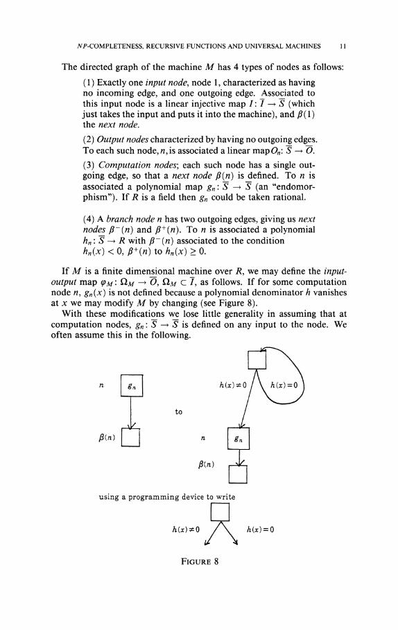
The directed graph of the machine M has 4 types of nodes as follows:
( 1 ) Exactly one input node, node 1, characterized as having no incoming edge, and one outgoing edge. Associated to this input node is a linear injective map 1:7 —• S (which just takes the input and puts it into the machine), and /?(1) the next node.
(2) Output nodes characterized by having no outgoing edges. To each such node, «,is associated a linear mapO„: S —• O.
(3) Computation nodes; each such node has a single outgoing edge, so that a next node P(n) is defined. To n is associated a polynomial map gn : S —• S (an "endomor-phism"). If R is a field then gn could be taken rational.
(4) A branch node n has two outgoing edges, giving us next nodes p~{n) and P+(n). To n is associated a polynomial hn: S —• R with p~{n) associated to the condition hn(x) < 0 , 0+(n) to hn(x)>0.
If M is a finite dimensional machine over R, we may define the input-output map (PM '- QM —• 09 QM C / , as follows. If for some computation node n, gn(x) is not defined because a polynomial denominator A vanishes at x we may modify M by changing (see Figure 8).
With these modifications we lose little generality in assuming that at computation nodes, gn : S —• S is defined on any input to the node. We often assume this in the following.
en
Pin)
h(x)*0
to
Aid
PM r-^kl
using a programming device to write
h(x)*0 h(x) = 0
FIGURE 8

12 LENORE BLUM, MIKE SHUB AND STEVE SMALE
Let a machine M over R be given and let y e 7. The computation on y by M goes in a natural way. First I(y) G S and we are at node 1 in the computation process. If /?(1) = n is a computation node, the computation g„ is performed on the state x = I(y) to produce gn(x) which replaces x. If « is a branch node, and hn(x) < 0, the next node is P~(n). Otherwise the next node is fi+(n). In both cases, the next state is still x. Thus the computation proceeds until an output node n is reached (if ever) and On(x) for some x e S is computed. In this case the computation is said to halt and produces (pM{y) — On(x). Denote £IM C / as the set of y where the computation halts. QM is t̂he halting set of M. Thus M defines the input-output map q>M '> &M —• O. Compare the example of § 1, which essentially are finite dimensional machines over R.
It is important to allow infinite dimensional machines in the construction of universal machines and to analyze uniform algorithms (algorithms which solve problems with inputs of arbitrarily large size).
We now discuss the modifications needed in the finite dimensional machines tojnake them infinite. In an infinite dimensional machine we take ƒ = Rl, O = Rm now allowing /, m to be < oo, together with a (finite) directed graph. The 4 nodes as before are the same from a graph theoretical view, but the definition of the associated maps must be extended to cover the oo-dimensional case. We have already defined a polynomial map R°° —• R°°. But this will not affect Xt for large / in the expression x = (x\9X2,... ) G R°°. This consideration forces us to introduce another type of node into the machine which we call a fifth node. A fifth node is designed to access the xt with large /. For this we take S = Z+ +Z++R00 with a typical element {i,j,x\,X29...), i,j positive integers. A fifth node (one outgoing edge and unique next node fi{ri) as in a computation node) operates on this element by transforming it to the element (/, j,x\,X2,...,xt replacing Xj in the y'th place in i?°°,... ) G S. No other changes are made in the computation of_a fifth node. If n denotes this node, then that map will be written as gn : S —• S.
In the oo-dimensional case the input map I: I —> S = Z+ + Z+ + R°° can conveniently be taken as follows: non-zero-coordinates are given by I(xhk+\ = xk for k < I leaving starting values i = 1,7 = 1 in the Z+ + Z+
part of S. This leaves "working space" in S. For technical reasons, we also assume coordinate 7(x)4 denotes the
length of x. Here, the length of a nonzero element x e Rl is defined as the largest k such that x^ ^ 0; the length of the 0 vector is 1.
The gn : S -> S of a computation node is required to be of the form gn(i,j,x) = (ï(ij)j'{ij),x'{ij,x)) with i'(ij) = /+ 1 or 1. (Similarly, f(i,j) = j+1 or 1) and x'(i,j\x) satisfying the previous defined condition for polynomial (or rational) maps on oo-dimensional spaces. The branch node polynomial h : Z+ + Z+ + R°° —• R, we suppose satisfies dh/dxt = 0, i > some k. (This condition defines a polynomial function.) We let kM denote the maximum dimension of the maps and functions associated with the computation and branch nodes of M. Similarly, dM is the maximum degree of these maps.
JVP-COMPLETENESS, RECURSIVE FUNCTIONS AND UNIVERSAL MACHINES 13
The final modification for the oo-dimensional case is on the output map On\ S —• O. Suppose it to be of form On(iJ,x)k = x2k-\, k = 1>2, —
The input-output map CM for the infinite dimensional machine M is defined just as in the finite dimensional case. For /, m < oo we say that a (partial) map (p: Rl —• Rm is computable over R iff there is a machine M over R such that QM = &><p, the domain of <p, and Ç>M(X) = (p{x) for all x € Cl<p. In such a case we say M computes <p. Machines M and M' will be called equivalent if they compute the same map.
A set Y c Rn will be called R.E. over R if Y = ftM for some machine M over /?. It will be said to be decidable if it and its complement are both R.E. over R. It is an easy exercise to show that Z is a decidable subset of R over R for any Archimedean ring R.
Sometimes it is convenient to restrict the inputs of a machine from 7 to a subset Y c 7. Thus Y would be considered the space of admissible inputs (for some problem, for example). Various notions in our theory may be relativized to such a space of admissible inputs. For example, if Y c / let QM,Y = &M n Y. Then we would say £IM,Y is an R.E. set over R relative to Y.
It is also convenient often to view Rk as being contained in Rl for k < / < oo via the natural injection j : Rk —• Rl where j(x) = (x, 0 , . . . ) , / - k zeros after x. Thus, e.g. we may think of ( 1,0,0,... ) G R°° as the element I E R{ C R°°. In the infinite dimensional case, it is often useful to write R°° = R°° + + R°° (m times) in 5.
When we talk about a machine over R in the sequel, this could mean either the finite dimensional or the infinite dimensional case. For x E S we will sometimes use the notation x]^, k = 1,2,... to denote the Arth coordinate of x in the finite dimensional case, and the k + 2 coordinate of x if S is infinite dimensional. In the latter case, x]_i,x]o will denote the first 2 coordinates of x respectively.
3. The computing endomorphism and the register equations. In this and the following two sections we develop the machinery and concepts needed to prove our Main Theorem on TVP-completeness in §6.
First of all, we define a machine over R to be in normal form if it satisfies: _
(1) At each branch node, n, hn(x) = x]\, for x G S. This is a minor condition making things a bit more convenient.
(2) There is one output node, and hence one output map O: S —• O. (3) There is a given labeling of the nodes {1,2,..., TV} such that
(a) 1 labels the input node, (b) N labels the output node.
(4) In the finite dimensional case, I is the natural injection and O is the natural projection.
PROPOSITION 1. Given any machine M over R, there is an equivalent one in normal form.
PROOF. One achieves property ( 1) by adding a computation node before and after each branch node using a little straightforward programming

14 LENORE BLUM, MIKE SHUB AND STEVE SMALE
exercise. To obtain (2), one just collapses all of the output nodes to a single one. (And in the finite dimensional case, perhaps expand the state space and number of nodes a bit to obtain On = O.) The existence of the labeling (3) is clear. For (4) we add computation nodes immediately after the input and before the output nodes.
Forji machine M over R in normal form, there is a natural map H = HM from N_ x S to itself, called the computing endomorphism of the machine. Here N = {1,..., TV} is the set of nodes and S is the state space. We call N x S the full state space of M.
The computing endomorphism H: NxS —• NxS has the form H(n, x) = (fi(n>X(x)), gn(x)) where ƒ? describes the next node and gn the new state. Here x ' S —• R is defined by
!
1 i fx ] i>0 , 0 i f x h = 0 ,
- 1 i fx ] i<0 .
We define ft : TV x {0, ±1} —• ~N as follows, depending on M:
{ N if n = N, P(ri) if n < N and n is a nonbranching node, (3+(n) if n is branching and a = 0 or 1,
^ fi~(n) if n is branching and a = - 1 .
0{n,a)= {
To define gn as a function of n and x, let gn(x) = x for n = 1, JV or a branch node. At a computation or fifth node we suppose gn{x) is the computation given by that node.
Thus the computation of a machine M over i? with input y e I is represented by a sequence z0, zi, Z2,..., zk,... for zk G TV x S, z$ = (l,/(y)) and H(zk_x) = zk, k = I, In dynamical systems terminology, this sequence of zk = (nk,xk) is the orbit of the computing endomorphism with starting point zo. Note that if M is infinite dimensional and xk = (/, j , . . . ), then /,y < k.
We remark that if gn is a rational map, then gn(x) may not be defined for some x e S. Thus H is a "partial" map. However, by starting with z0 = (\,I(y)) we are assured (by our convention on machines) that H can be iterated without concern.
A necessary and sufficient condition that a sequence z0, z\,... be a computation by the machine M is that
(la) zk = H(zk_{), fc=l,2,...
and secondarily, z0 = (fto>*o) has the form
(lb) «o=U *o = I(y), for some y G 7.
Let us call equations (la),(lb) the register equations of the machines M. Equation (la) may also be written
(la') P(nk-ux(xk-i)) = nk gnk_{{xk.x) = xk for k = 1,2,....

WP-COMPLETENESS, RECURSIVE FUNCTIONS AND UNIVERSAL MACHINES 15
Input y il
z = (n,x) is replaced by H(z) z^-H{z)
Output
F I G U R E 9
In the sequel, symbols such as n^ or x^ will sometimes represent specific elements (in N or S say), and sometimes variables. The intended usage should be clear from context.
One can represent the computation process of a machine over R by the following flow chart. (See Figure 9.) (Compare this flow chart with the "Julia set machines" of §§1 and 10.)
Thus for given y, one keeps computing H until node N is reached in which case the machine outputs O of that x in S.
For reasons to become apparent in the next sections, we move to putting the register equations of a machine M over R into a more algebraic form. To do this we first put the computing endomorphism into a more algebraic form, at the same time extending it to an endomorphism of R' x R'n. Here R' is the ring generated by R and Q and, in the infinite dimensional case, R'n is to be interpreted as R'+ R'+ Rfoc (similarly for Rn).
LEMMA 1. fi can be extended to a polynomial map {also denoted) fi : R' x R' -• R' of degree N + 1.
PROOF. For each n e N, let
an(y) TT ^ ^ . tfnjeN
So, for y e N,
an{y) -{J if y = n,
0 if not.

16 LENORE BLUM, MIKE SHUB AND STEVE SMALE
Let B = {branch nodes of M}. Then
p{y,a)= Ç a „ ( j ; ) ^ ( „ ) + ^^±ü + (C T + i ) ( i_ ( T))^ a n(^+(„) n€N-B "€fl
+ aJa-VL^an{y)r{n)
neB
(Note that P{n,a) is independent of o for all nonbranching nodes n.) It can be easily seen that the degree of /? is N+1 and that /? can be written as a sum of 67V monomials in the variables y and a.
Now let g(n,x) = gn(x). As above, we can extend the definition of gn(x), or equivalently g(n,x), to all n in R.
A formula for this is
g(y>x) = ^2an(y)gn(x), nëN
an(y) as in the above proof. Suppose R is a field and the computation at node n takes the form
gn'
Here pln(x), ql
n{x) are polynomials if n is a rational computation node; otherwise, pl
n(x) = gln(x), the /th coordinate of g, and ^(x) = 1. Then
the above is modified simply to
,(v . = EneN"n(y)pln(x)
Since ^2neN an{y) = 1 for y € N, the previous formula is recovered for
y e N, whenever qln{x) = 1, all « e TV.
It is clear that if M is finite dimensional, then g is a polynomial (or rational) endomorphism of R' x R'n. This is not necessarily the case if M is infinite dimensional due to the existence of fifth nodes.
Nevertheless, if M is infinite dimensional, it is the case that for each k e Z+, there is a polynomial (or rational) endomorphism g^ of R' x Rfn of dimension Kk that is identical to g on N x S^y Here K^ = max(/cvv/, k + 2) and 5(fc) = {(/,.ƒ...) € 5|/,7 < A:}. Furthermore, these endomorphisms are uniform in k. This will follow from the above together with
LEMMA 2. There is a universal map F: Z+xRfn —• R'n such that for each k G Z+, F(̂ ) (= F(k9 •)) w a polynomial endomorphism ofR'n of dimension k + 2, degree 2k - 1 a«J F^k) is identical to the fifth node computation on
PROOF. Let a: Z+ x Z+ x Z+ x R' x R' ^ R' be defined by
«*.«...»>- n (£f) n (fff) P€*-{*} qek-{j}
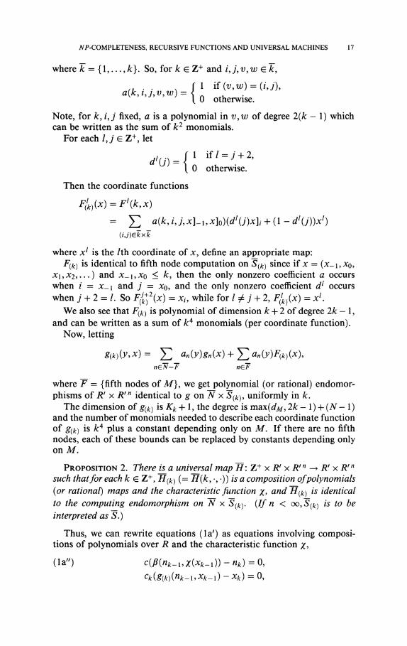
JVP-COMPLETENESS, RECURSIVE FUNCTIONS AND UNIVERSAL MACHINES 17
where k — {1,..., k}. So, for k e Z+ and /, j , v,w ek,
n . . v ƒ 1 if (v,w) = (i9j), a(k,i,j,v,w) = i { 0 otherwise.
Note, for k, i,j fixed, a is a polynomial in v,w of degree 2(k - 1) which can be written as the sum of k2 monomials.
For each IJ e Z+, let
dil') = ( 1 ifl = j + 2> U) \ 0 otherwise.
Then the coordinate functions
FJk)(x) = Fl(k,x)
= £ *(k>i>J\x]-i,x]o)(dl(j)x]i + (l-dlU))xl) (ij)ekxk
where xl is the /th coordinate of x, define an appropriate map: F(fc) is identical to fifth node computation on S ^ since if x = (x-\,x0,
X\,X2,...) and X-\,Xo < k9 then the only nonzero coefficient a occurs when i = X-\ and j = xo, and the only nonzero coefficient dl occurs when j + 2 = /. So i ^ C * ) = xi9 while for / ̂ y + 2, / ^ ( x ) = x7.
We also see that F^ is polynomial of dimension k + 2 of degree 2A: — 1, and can be written as a sum of k4 monomials (per coordinate function).
Now, letting
g{k){y,x)= ] T an(y)gn(x) + Yl<*n(y)F{k)(x), n€N-T n€F
where F = {fifth nodes of M}, we get polynomial (or rational) endomor-phisms of R' x R,n identical to g on N x S^), uniformly in k.
The dimension of g^ is Kk + 1, the degree is max(rf^, 2/c - 1 ) + (N - 1 ) and the number of monomials needed to describe each coordinate function of gft) is k4 plus a constant depending only on M. If there are no fifth nodes, each of these bounds can be replaced by constants depending only on M.
PROPOSITION 2. There is^a universal map H\ Z+ x R' x R'n -+ R' x R'n
such that for each k e Z+, H^ (= H(k, -, •)) is a composition of polynomials (or rational) maps and the characteristic function x> and ~H{k) is identical to the computing endomorphism on N x S^y {If n < oo,S(k) is t0 be interpreted as S.)
Thus, we can rewrite equations (la') as equations involving compositions of polynomials over R and the characteristic function x,
(la") c(0(nk_ux(Xk-i))-nk) = O, Ck(g(k){nk-i>xk-i)-xk) = 09

18 LENORE BLUM, MIKE SHUB AND STEVE SMALE
for k = 1,2,..., where c, ck are the (smallest) positive integers sufficient to cancel denominators. (If n < oo, g^) is just g.) In case M has rational computation nodes, we replace the second set of equations by the coordinate polynomial equations:
Ck\ Yl Mnk-\)pUxk-\) + Ylan(nk-^F(k)(xk-i) \neN-T n€F
-x[ J2 an(nk-i)qln(xk-i) = 0.
nelv J
Note that the coordinate equations of the second set for I > Kk can be written as x[_{ - x[ = 0.
Now suppose R is a field with the property that any positive element is a square. Thus R could be the real numbers or any real closed field. With R satisfying the property we can eliminate the characteristic function x in
the above and thus put the register equations into an even finer algebraic form.
To do this we introduce new variables U\,ui,...,uk,... for k = 1,2,... and replace (la") by the following polynomial equations over R.
(la"') **-i]i(**-i]iwjfc-i + W ^ - i W - i - 1) = 0
P{nk.uxk^]xu2
k_x) - nk = 0
8{k)(nk-uXk-\) ~ xk = 0
for k = 1,2,.... Again, if M has rational computation nodes, the last set of equations
can be modified appropriately.
PROPOSITION 3. Suppose the field R has the property that positive elements are squares of elements in R, and suppose M is a machine over R. Then the sequence (no,xo)9 (n\,X\),... {nk,xk) e Rx Rn is a computation by M if and only if it satisfies (la"') for some u\,U2,.-. in R and (lb). If these conditions are satisfied then necessarily (nk,xk) e N x S.
The proof is straightforward. We can characterize computations via polynomial sets of equations and
(lb) even more generally. For example, if the field R has the property that every positive element is a bounded sum of squares (e.g., by Lagrange, every positive rational number is the sum of 4 squares of rationals) we can replace every occurrence of u\_x above by 2/=i u}k-i)j where b is the given bound and u^-\)j a r e n e w variables for j = 1,..., b and k = 1,2,

JVP-COMPLETENESS, RECURSIVE FUNCTIONS AND UNIVERSAL MACHINES 19
Over the ring of integers, we can replace (a") by
c lxk-ih -Y^u2{k-\)j ~ X I I xk-ih +^2uîk-i)j+l I [P(*k-\>xk-i]\)-nk\ = 0
4 \ / / 4
<**-i]i l ^ - i l i - ^ " ( i t - i ) y - 1 ) Ifi ( H*-i,**-ih +XX*-')y ) ~ ^
and ^ ( ^ ) ( ^ - i , ^ - i ) - ^ ) = 0
where U(k-\y are new variables for 7 = 1 , . . . , 4 and A: = 1,2,
4. Time 7* halting sets, equations, polynomials and computations. Let us consider now halting computations, i.e., those sequences (nk,Xk) satisfying (la7) or (la"), (lb), and with the added condition HT = N for some T < 00. Such a T will be called a halting time for the y in (lb) and the halting time for M to compute <p\t{y) will be denoted by TM{y) or T(y) and is the minimum T such that «r = N. If T = T(y), we then have the pair of equations satisfied:
(lc) nT = N, 0{xT) = (pM{y),
(O the output map). Let 7T_ = {y G 7\T(y) < T} be the time T halting set of M. Thus,
QM — U 7r> the union over T eZ+. We remark that if y, y G / agree on the first KT = max(/cM, 7" + 2) coordinates, and y G 7^, then yf G 7> and 9M{y'), (phf{y) agree on the first KT coordinates.
We now consider the time T halting equations
(la') or (la") for k= 1,. . . ,T, (lb') n0= l,x0 = I(y), (lc') nT = N.
We can use these equations to get algebraic descriptions (modulo x) f ° r
various relations. For example, let GM,T = {(y,w) e Rl x Rm\w = ç>M(y) and y G IT} be the time T graph O/ÇM- Then,
(y,w) G GM,T if and only if there is a a = ((«o>*o)>---(«r, Xr)) G (R x Rn)T+l such that (y, cr, w) satisfy the time r halting equations p/ws w = 0(XT).
(As before, we interpret Rn as i? + R + i£°° in the infinite dimensional case.)
If M is finite dimensional, these equations are polynomial, modulo the characteristic function x, and finite. If M is infinite dimensional they

20 LENORE BLUM, MIKE SHUB AND STEVE SMALE
are not finite, nor are I and O polynomial. However, for each T, we can easily modify the time T halting equations to get a finite polynomial system (modulo x) by eliminating all j coordinate equations from the second set in (la") and (lb'), for j > KT = max(kM, T + 2). We then have
(y,w) G GM,T if and only if there is a o e (R x RKT)T+I such that (y9<j,w) satisfy the "modified" time T halting equations plus
( xrhj-i fov2j<KT-\, J {yj fov2j>KT-l.
Note, the only nonfiniteness comes in the last equations, and then only in a nonessential way.
Over the reals, the time T halting equations are equivalent to a polynomial system (just replace (la') by (la'") for k — 1 , . . . , T). By modifying this system as above we get a finite polynomial system.
We can now use the following proposition to convert this system to a single polynomial equation of degree less than or equal to 4 which we call the time T halting polynomial equation for M.
PROPOSITION 1. Over the real numbers, (a) any system of polynomial equations is equivalent to a quadratic sys
tem. (b) Any quadratic system is equivalent to a single equation of degree less
than or equal to 4.
Here equivalence means if one system has a solution then so has the other.
For the proof of (a), consider the polynomial equation Y,a aaxa = 0,
a = ( a i , . . . , a „ ) , a/ nonnegative integers. Let ta = xa be new variables. One has an equivalent system for the ta
9s of the type ta+p = tatp together with 2 a aata = 0, a ranging over some set 7.
For the proof of (b), one just takes the sum of the squares.
THEOREM. Let R = R and let M be a given machine over R. For each T e_Z+, there is a polynomial fr'. R*r x R ^ R of degree < 4 such that y elr if and only if there is a z e Rs such that fr(yu> • •, yKT>z) — 0.
Furthermore, s (and the number of monomials needed to express fr) is bounded by a polynomial in T, depending only on M. (If the input space is finite dimensional, we replace KT by /, the dimension of the input space.)
PROOF. The existence of a single polynomial follows from the above discussion and Proposition 1. (z encompasses all the variables in the "modified" time T halting equations, except in y, plus the variables needed to eliminate x as well as those needed to convert the system into a quadratic one.) To get the polynomial bound on the number of variables (and monomials) we must count the number of variables and monomials appearing in the modified time T halting equations, the number of new variables (and equations) needed to get a quadratic system (and then the number of monomials needed to describe the resulting quartic equation). These

W-COMPLETENESS, RECURSIVE FUNCTIONS AND UNIVERSAL MACHINES 21
counts are mainly affected by the number of monomials needed to describe the "fifth node" polynomials f^ for k = 1,..., T. One thus uses the analyses given in §3 to get a requisite polynomial bound.
Observe that the construction of the polynomial fr above is uniform in both T and M. We can restate the Theorem to reflect this, and in a somewhat different way.
THEOREM'. There is a machine over R which on input (M, T) (where M is a machine over R and T e Z+) outputs in time polynomial in lM [the 'length ofM') and T, a polynomial fMJ\ RKT X BP°WM,T) _+ R 0f degree < 4 satisfying the following diagram
V = f~]T(0) c R*r x RP°iy(/"T) ^ i R
lMj = n^nx{V) c R°°—>R^
Here 7M,T is the time T halting set of M and n\, 712 are the projections of RKT x RP°1y(/A/'r) and R°° onto RKT respectively.
(If the input space is finite dimensional, replace KT by the dimension of 1M and ignore 7r2.)
To make sense of Theorem', we have to define the "length of M" and specify how machines M and polynomials ƒ over R are to be represented in R°°. This will be done more precisely in the next sections. Polynomials will be specified by their "powerfree" representations (see §5) and machines by their programs (see §8). The "length of M" will then be the length (as defined in §5) of the representation in R°° of the program for M.
We now develop the relationship between the time T halting sets IT and the time T halting computations TT. Here FT = TM,T is the subset of (R x S)T+l consisting of ((no,xo),..., (HT9XT)) satisfying, for some y e 7, the time T halting equations. (Note we automatically get that y e IT and o(xT) = (pM(y).)
There are natural maps a, a' defined as follows:
IT —• TT —• IT,
a{y) = ((IJ(y)lH(lJ(y)), H2(l9I(y)),...9HT(l9Hy))) and
af((n0,xo),...,(nT,xT)) =y
where «0 = 1 and x0 = I(y). Then a and a' are inverses to each other and provide a set-theoretical
isomorphism between IT and TT. Moreover a' is continuous and even is the restriction of a linear map. But a in general is not continuous, since H is not (recall H involves a characteristic function).
Now consider the map y\ : TT —• RT+{ which is the restriction of the projection (RxS)T+l -> RT+l. In fact yi(TT) c ÏVr+1 c RT+l. Define
_ T+\ y: IT —> N as the composition y{ • a. One can interpret y(y) as a halting path or as the computation path of y of length T in the directed graph of the machine M. So y(y) is the sequence of nodes traversed in

22 LENORE BLUM, MIKE SHUB AND STEVE SMALE
T+\ —
the computation ç>M(y). If y € N , let Vy be the subset of IT such that y(y) = y. Then it is easy to see that a restricted to Vy is a continuous map from Vy into TT>
PROPOSITION 2. (a) Vy is a semialgebraic subset O/7T, (basic, if the maps at computation nodes are polynomial), and Ç>M restricted to Vy is a rational map.
(b) IT — UyEA^1 Vy is semialgebraic. The Vy 's are disjoint. (c) QM = \JT>O^T is a countable union of semialgebraic sets.
PROOF. Only (a) needs proof. By following the path y and noting the branches taken, one sees that Vy is defined by inequalities of the type
gkl{'--gkMkx{I{y))))]i<Q and ^(•••& 2 (a 1 ( / (y))) ) ] i<0
where the g's are polynomial (or rational). If the g's are rational, each inequality is replaced by a disjunction of polynomial inequalities by using the correspondence: p/q < 0 iff (p < 0 and q > 0) or (p > 0 and q < 0). Similarly, by composing the computations along the path y, one can see that (pM restricted to Vy is of the form Ogjn(- • • gj2{gj\ (I(y)))).
If M is finite dimensional we are done. If M is infinite dimensional, we can, as in the modified T halting equations, use the bound KT on the number of "active" coordinates and variables in a computation of length T to get semialgebraic descriptions of Vy, and polynomial (or rational) descriptions of Ç>M restricted to Vy.
Note that M with inputs restricted to IT is essentially a finite dimensional machine. Moreover, this machine is equivalent to one without loops, a tree as in Smale.
We remark that (b) gives an algebraic description of IT via an exponential (in T) number of semialgebraic formulas. Compare this with the time T halting polynomial description of IT given by the previous theorems for the case R = R.
As discussed in § 1, it follows from Proposition 2 that Julia sets in general are undecidable. There are other immediate applications. For example, we now easily get a lower bound on the halting time for computing the "greatest integer in." (See Example 5 in §1.)
PROPOSITION 3. Suppose a machine M computes \x\ for x e R+. Then TM(X) > log(x) for an unbounded set ofx.
PROOF. Fix such a machine M. For each LeZ+ let TL be the maximum of the halting times TM(x) for x < L, x e R+. (We can suppose TL < oo.) So for x < L, x e R+ we have x E7TL, which is the union of at most 2TL
sets Vy, y of length TL. On the other hand, for each nonnegative integer /, there is an open set
U of points in R such that for all x € U, Ç>M(X) = /• If I < L, there must be such an open set in Vy for some y of length TL. But Ç>M restricted to Vy is polynomial (or rational). So, CM restricted to Vy must be identically equal to /. Thus, there must be at least L such sets Vy.
So2r^ >L , i.e., TL >logL.

WP-COMPLETENESS, RECURSIVE FUNCTIONS AND UNIVERSAL MACHINES 23
In a similar fashion, we get lower bounds for the Travelling Salesman Problem over R. (See Example 7 in §1.)
Suppose M solves the TSP over R, i.e., for each mileage chart A over R> <PM(A) is a tour of minimum distance. (Of course, we are supposing 1 — O — R°° and some specified representation of mileage charts and tours in R°°. For example, an n x n matrix A could be represented in R°° as n followed by a listing of the rows of A. A tour t of n cities could be represented as an ordering (z'i,...,/«) of the integers 1,..., n where i\ = 1. Thus, t(ij) = ij+\ for j = l,...,n - 1 and t(in) = 1.) For n e Z+ let TM{n) — max TM(A), where A ranges over all n-city mileage charts over R. The topological complexity of M, as a function of n, is the number of halting paths of length TM(n).
PROPOSITION 4. Suppose M solves the TSP over R. Then the topological complexity of M is at least (n - l)!/2. So
TM(n) >\og^^.
The proof is similar to above, noting that for each tour t, there is an open set of inputs U such that for all A e U, <PM(A) = t or 1 (where t is the reverse of t). So, there must be such an open set in Vy for some y of length TM(n). So, since Ç>M restricted to VY is polynomial (or rational), we have (J>M restricted to Vy identically t or t. The result now follows since there are (n - l)!/2 (unoriented) tours over n cities.
The topological complexity of the TSP measures the branching necessary and sufficient to solve all «-city instances. (It could be thought of as the "obstruction" to obtaining a rational formula solution.) This notion can be studied more generally. For example, a slightly more subtle argument shows the topological complexity of the Knapsack Problem over R is 2n. (The Knapsack Problem is: Given (x\9...,xn) eR". Find a subset S ç {1 , . . . , n} such that J2tesxi = 1» if o n e exists.) For lower bounds on the topological complexity of solving 1 variable polynomial equations, see Smale.
REMARK. In the above two examples the machines compute functions that take values in a discrete set. We used open set arguments to get estimates on the number of components Vy of IT, thus getting our lower bounds. If these open set arguments were not applicable, we could still use estimates on the number of connected components of IT (see e.g., Milnor and Thorn) to get lower bounds.
5. Complexity theory of machines over R. A background reference for this section and the next is Garey-Johnson, which gives an account of the ideas of TVP-completeness of Cook and Karp. Here we are considering a version of this theory, more algebraic and especially over the real numbers. There are some differences in substance.
Toward defining the property, "a machine M over a ring R is in class P" (polynomial time), we introduce the notion of size. The length of a nonzero element x G Rn (n < oo) is defined as the largest k such that Xk 7̂ 0, where x — (x\, xi,..., xk, 0,0,... ). The length of 0 is 1. The size

24 LENORE BLUM, MIKE SHUB AND STEVE SMALE
of x is to be the length of x plus the height of x where the height is yet to be defined. The height of x is the maximum of the height (x,-) over all /, and it remains to say what the height is for an element of R. We only do this here for the cases R = Z the integers, Q the rational numbers and R the real numbers. If R = Z, x e R, then height x = log(|x| + 1). If R = Q, x = p/q e R, p,q relatively prime integers, then height x is the maximum of height /?, height q. Finally if R = R and x e R, then height x — 1. Note the difference in the case of x e Q c R depending on which field is considered. For some other rings R, the notion of height (e.g. Mazur) from algebraic number fields is suggestive.
The height over Z of an integer is essentially the number of bits. The height over R reflects the fact that as in scientific computation, the cost of multiplication is independent of the magnitude of a real number.
PROPOSITION 1. Let M be a machine over R and for y el, let TM(y) be the halting time as in the previous section. Then a(y) < kTM(y) where a(y) is the number of arithmetic operations and uses of 5 th nodes used to compute <pM(y)- The constant k depends only on the machine M.
The proof is straightforward from the fact that M has only a finite number of nodes. Thus, there is a bound on the degree and the number of active variables and coordinates over all the computations at nodes.
We now define the standard cost function C^CF) of machine M on input y to be the product of the time, TM(y), and the maximum height, hM(y), occurring in the computation of <PM(y)- That is,
liM(y) = max height^) where Hk(l,I(y)) = (nk,Xk) some n^ e N. 0<k<Tm(y)
where x'k is identical to xk on its first kM coordinates, 0 elsewhere. Note that for R = R, CM (y) = TM(y). For R = Z, CM (y) is poly normally related to the "bit complexity" of computing <PM(y)-
Now say that a machine M over R is in class P {polynomial time) (or that the computable function <PM is in class P over R) if there are constants c and q e Z+ such that
CM(y) < c(size(y))q all y G 7.
Here and in what follows, often sense is made only in case height has been defined. This includes R = Z, R at least. For R = Z, class P over Z is identical to the classical polynomial time class with respect to the bit complexity measure of cost.
Suppose Y c 7 is a space of admissible inputs. We say that the pair (M, Y) is in class P if
CM(y) < c(size(j/))« all yeY.
A decision problem over JR is a pair (Y, Yyes) where Yyes c Y c 7 = Rn, n < oo. A problem instance is a point yeY, with question: "Is y in YyesT" This formulation of a decision problem equates it with a membership problem.

NP-COMPLETENESS, RECURSIVE FUNCTIONS AND UNIVERSAL MACHINES 25
An algorithm (or sometimes machine) which solves a decision problem (Y, Yyes) over R is a pair (M, Y), where M is a machine with space of admissible inputs Y such that (pM{y) = 1 (yes) or 0 (no) for all y G Y, and <PAf(y) = 1 if and only if y G Yyes.
Then we say that the decision problem ( Y, Yyes) is in class P if there is an algorithm in class P which solves it.
PROBLEM 5.1. Would the class of decision problems in P over Z increase if the cost function were changed to TM(y)r! (Certainly, the class of polynomial time computable functions over Z would increase, e.g., consider the function ƒ(*) = |*lw«)
We will say that a decision problem (Y,Yyes) over R is in class NP (nondeterministic polynomial time) if there are constants c and q e Z+
and a machine M over R with 7^ = 7 x 7 , where 7 = 7 = Rn, n < oo and the space of admissible inputs for M is Y x 7 , such that
(a) the values of Ç>M are 1 (= yes) and 0 (= no). (b) q>Miy,y') = 1 only if y G Yyes and, ^ (c) for each y e Yyes, there is a j / G 7 such that ^AfO>,J>') = 1 and
C^(y,/)<_c(sizeö;))^ The y' e I are the guesses as in the standard ATP-completeness theory
(see Garey-Johnson). It is easy to see that without loss of generality we can assume, in (c) that the size (y') < c' size (y)q, for some fixed c' G Z+. Again, if R = Z, our class NP coincides with the classical one.
PROPOSITION 2. NP D P over R.
The proof goes by using the machine for P and ignoring the guess. The following two examples illustrate our notion of NP over the real
numbers R.
PROPOSITION 3. The Traveling Salesman decision problem over R is in NP.
(See Example 7 in §1.) PROOF. We write a flow chart for the NP machine as follows (Figure
10):
((M),/) Here: k€R,A is a "mileage chart", and y'€I, a guess
Here: D(A,y') denotes the distance of tour y'.
F I G U R E 10

26 LENORE BLUM, MIKE SHUB AND STEVE SMALE
The proof now focuses on the subroutine, "Is y' a tour?" Suppose mileage charts and tours are represented as in §4. Let n be the number of cities. To check if y' represents a tour of n cities just check if each integer 1,...,« appears once and only once in (y[,...,yf
n) and y[ = 1. Now it can be seen that the subroutine can be implemented by a polynomial time algorithm.
The second example is the 4-Feasibility problem, a certain feasibility problem for real algebraic varieties, which we write (F,Fyes). Here F consists of polynomials ƒ : R" —• R of degree < 4, and ƒ G Fyes if there is some x eRn such that f(x) = 0. It remains to be specified how F c R°°. To do this we describe the powerfree representation:
The polynomial ƒ : R" -> R of degree < 4 is powerfreely represented in R°° as (4, n) followed by a sequence of (a,aa) where a = (01,0:2,0:3,0:4), ai G [0 , . . . , « ] , o/ < ai+\ and aa G R. The pair (a,aa) stands for the monomial aaxaixa2xa3xa4, with xo = 1 to allow for terms of degree less than 4. These (a, aa) are supposed ordered by the lexicographic order on the o. Thus f(x) = E a ^ ^ i ^ ^ ^ ' Note ƒ can be considered as a polynomial on R°° which does not depend on xt for i > n. (For each degree d G Z + , it is clear how to generalize this description to get the powerfree representation in R°° of polynomials ƒ : Rn —• R of degree < d.)
PROPOSITION 4. (F,Fyes) is in NP over R.
The NP machine takes guesses for ƒ : Rn —• R, points y' in R°° and tests if f(y') = 0. Since degree ƒ < 4, this evaluation is given by a polynomial time machine.
PROBLEM 5.2. Does P = NP over R?
6. TVT-completeness and the analogue to Cook's theorem over R. Inspired by the theory of NP completeness in computer science (see Garey-Johnson) we say that a decision problem (7 , Yyes) is NP complete if it is in NP and: Given any decision problem (7, Yyes) in NP, there is a map y/:Y^Y with these properties:
(a) y/(y) e Yyes if and only if y G Yyes. (b) y/ = (PM\Y for some machine M, and this machine is in class P. In
other words y/ is polynomial time computable. This definition is meant over a ring R and a definition of height over
R is needed. In particular, this is satisfied if R = Z in which case our definition checks with the classical definition. Also the case of R = R is included, in which case, we have a new definition of NP complete. This is the case of primary interest in what follows; but the case of real closed fields should be the same.
MAIN THEOREM (ANALOGUE OF COOK'S THEOREM FOR R). The 4-
Feasibility problem (F,Fyes) of the previous section is NP complete over R.

^^-COMPLETENESS, RECURSIVE FUNCTIONS AND UNIVERSAL MACHINES 27
The proof uses the machinery and results of the last three sections. Note first that (f7, Fyes) has already been proved to lie in NP, Proposition
4 of the previous section. Let M be the "nondeterministic machine" in the definition of NP for the problem (Y, Yyes). In this definition there is the polynomial bound c(size(y))q = T0(y). We must describe the map y/\ Y —• F with^the requisite properties. Thus let y e Y and consider in the space (R x S)T+l, T = T0(y), the equations (a"') for k = 1,..., T. We adjoin to this set, the following
(2) « o = l , I{y,y') = Xo. (Here y' is a free variable of length KT.) (3) nT = N, and 0(xT) = 1 (yes).
LEMMA. For y e Y, this system of equations (la"'), for k = 1,..., T(2) and (3) has a solution if and only if y e Yyes.
PROOF. One just has to trace through all the definitions. This system is equivalent to the time T halting equations of §4 (now with
input space 7 x 7 ) plus the equation 1 - XT]\. Thus, it is easily modified to an equivalent finite polynomial system (we have already eliminated / ) .
As in the Theorem in §4, we can convert this system to a single polynomial equation ƒ : Rn —• R of degree less than or equal to 4, to obtain using the powerfree representation, y/: Y —> F. By the previous lemma, y/(y) is in Fyes if and only if y G Yyes. It remains to see that y/ is a polynomial time computable map.
For this one notes that the construction of y/ makes the computability clear. Moreover, since T = T0(y) is a polynomial in the size of y, it is only left to see that the length of (the powerfree representation of) y/(y) is a polynomial in T. Here one uses the analyses given in §§3 and 4.
COROLLARY. Any algorithm for the feasibility problem (e.g. from Tarski-Seidenberg, see van den Dries, or the faster algorithms of Canny andRenegar) can be used to solve any problem in NP over R. If that algorithm is a polynomial time algorithm, then any problem in NP over R can be solved in polynomial time.
This is a usual motivation for studying TVP-completeness (Cook-Karp) see Garey-Johnson.
Our theorem above raises many questions. Among them is: what are other A^P-complete problems over R? We only have very preliminary results in this direction as
PROPOSITION 2. Fixing a degree d, let F'd be the space of all semialgebraic sets defined by polynomial constraints of degree d, powerfreely represented. Let F'dyes be the nonempty ones. Then (F^Fdyes) is NP-complete.
PROOF. The reduction is given by the inclusion map F —• Fj.
PROPOSITION 3. Let F" be the set of all representations (powerfree) of polynomial systems of equations of the type trfj = t^, and one equation J2iej U — c- Let F"es be the feasible ones. Then (F",F"es) is NP-complete.
PROOF. This follows from the proof of Proposition 1.

28 LENORE BLUM, MIKE SHUB AND STEVE SMALE
REMARK. Finally note that the map ƒ : R" -* R, ƒ e F, gives a reduction to a one dimensional problem. Does 0 G Image ƒ ? (The image of ƒ is an interval. Of course the description of the interval is not the standard one.) This presumably can be defined as an TVP-complete problem.
7. Computable functions, normal forms and partial recursive functions over R. We deal mainly with the finite dimensional case. Suppose /, m < oo and let ƒ : Rl —• Rm be a partial function (map) computable over R. We denote this by writing ƒ e C^00. Suppose M computes ƒ. Added in proof. Without loss of generality we can assume M is finite dimensional.4 We may also assume M is in normal form. Using the (partial) computing endomorphism H\NxS-*NxS for M we get a normal form description for ƒ (and Ç>M)' f(x) = 0(h2(mmt(h\(t,x) = N),x)) where h\ : QAl = Z^° x 7 -+ TV and h2 : Slhl = Z^° x 7 -> S are given by Ai(f,Jt) = H'(1,I(X))}Ü and A2(f,.x) = ^ ( l , / ( x ) % and min,(Ai(f,.x) = TV) = min{* G Z^°|Aj(/,x) = N}. (Here, Z^° = Z+ u {0} and we are using the bracket notation as before to indicate projection. Thus ]^ means projection onto the first coordinate, and ]•§ means projection onto the remaining coordinates. Also, Hl means H composed with itself t times, H° is the identity.)
Inspired by this normal form description and by classical recursive function theory (e.g. see Davis, Manin, Cutland), we give a function-theoretic characterization of the computable functions over an arbitrary ring R.
DEFINITION. The class P£°° of finite dimensional partial recursive functions over R is the smallest class of partial functions (maps) f:Rl^Rm
(/, m < oo) together with their domains Qf, containing the basic functions: (i) the polynomial (rational, if R is a field) functions f:Rl^R (and
hence e.g. the successor, constant and coordinate projection functions), with their natural domains,
4In our original manuscript, we stipulated that M be finite dimensional in this definition, and posed the problem: Suppose a machine M over R has finite dimensional input and output space (but S may be oo-dimensional). Is M equivalent to a finite dimensional machine (one with dim S < oo as well)? We have with Leo Harrington answered this affirmatively, thus the class of computable finite dimensional functions remains the same with or without the condition that M be finite dimensional. The idea of the proof is to simulate M by a finite dimensional machine M'. The state space of M' has the same initial DM(= max(2/ + 2,2m + 2,kM)) coordinates as SM, then / coordinates to hold a (fixed) copy of input x G R1. In addition there is a coordinate to hold a single integer that will "code" at each stage the sequence of computations that if started on x € Rl will produce all current nonzero entries Xi of SM- The code uses prime powers and the node labels {\,...,N}. At each non fifth node stage in AT s computation, M' behaves as M on its initial coordinates, and also updates the code as necessary. At a fifth node stage in M's computation, with (i,j,X\,X2,...) G SM, if j < DM then M' puts x\ in the y'th place (if j > DM no replacement is made): If / < DM this is done by a polynomial map P^. If / > DM, then M reconstructs x7 from the (fixed) input and current code and the replacement is then made by a polynomial map Pj. (Several additional coordinates are used to construct and unravel the code and perhaps DM more for reconstructing x/.) The code is updated by replacing the sub code for the jxh place (given e.g. by the exponent of the y'th prime factor of the code) by the subcode for the Zth place. Subsequent to our solution, another was given by Harvey Friedman and Richard Mansfield.

JVP-COMPLETENESS, RECURSIVE FUNCTIONS AND UNIVERSAL MACHINES 29
(ii) the characteristic function x' &x = R —• {0,±1} where
!
- 1 if x < 0, 0 if* = 0, 1 if x > 0,
and closed under the operations of (a) composition, (b) juxtaposition, (c) primitive recursion and (d) minimalization. For (a) we suppose f:Rl->Rm and g: Rm —• Rn are given partial
functions. Then the composition g f: Rl -^ Rn is defined by g • f(x) = g{f(x)) where Clg.f = f~lng.
Next for (b), suppose ƒ• : Rl —• i?m' (/ = 1,..., k) are given and that y/ is the natural isomorphism mapping Rmi x • • • x Rmk onto Rm[+'"+mk. (We often identify Rmi x • • • x i?m* with i?m' +'"+m^ without writing y/.) Then the juxtaposition F = (fu...,fk): Rl -• jR'*i+-+'"* (0f the ƒ.) j s g j v e n by
F(x) = y/(f\(x),..., fk(x)) for x e Q f = f]^={Qfr Note that juxtaposition of polynomial functions gives us the polynomial maps f:Rl^Rm, (m = m\-\ h mic) and thus we also get the general projections.
For (c), we suppose we are given a partial endomorphism g: Rl —• Rl. Primitive recursion then defines a partial map G: Z-° x Rl —• Rl by G(0,x) = x and G(/ + l,x) = g(G(t,x)) and
QG = {(n,x) e Z^° xR l\n = 0ovn = t+l,(t,x) e Q,G and G(t,x) e fl^}.
So, for t e Z-°, G(t,x) = ^(x) = g £(x) (g composed with itself t times applied to x).
Finally, given F : QF D Z-° xRl -^ R, the operation of minimalization (d) defines a partial function L: i?; -+ Z^° where QL = {xe Rl\F(t,x) = 0 for some / e Z^0} and L(x) = min,(F(*, JC) = 0) = min{t e Z^°\F(t9x) = 0}.
Now suppose M is finite dimensional. Then the computing endomorphism for M is given by H(n,x) = (/?(«,xMi))>£«(*)) where ƒ? and #(«,-*) = gn(x) are polynomial (rational, if R is a field). (See §3.) Recall that the coefficients of /? and g are in the ring generated by R and Q. Since R need not contain Q, some modifications are necessary. We first define a partial recursive function over R which for x9y e Z-°, y ^ 0 gives the "greatest integer in" x/y: [x/y\ = mmt(F(t9x9y) = 0) where F(t,x,y) = x(y(t+ 1) — JC) — 1. Now, for n e ~N = {1,...,N} let
AnÜO = I l (y-y)x(y-j')
[(n-j)x(n-j)

30 LENORE BLUM, MIKE SHUB AND STEVE SMALE
Let
neN-B neB
neB
(As before i? = {branch nodes ofM}.) Now let ~g(y9x) = J2neN^n^Sn^' All the above functions are partial recursive over R. Thus (using the basic functions, composition, juxtaposition and the above), H:RxS-*RxS defined by H(y9x) = (P{y,x(x]\))>~ÏÏ(y>x) is partial recursive over i£. And also, H\j^ = H.
Thus H is a partial recursive endomorphism over R. So (using primitive recursion and appropriate projections in addition to juxtaposition, composition and noting that I and 0 are basic), we see that h\ and hi are partial recursive over R, each with domain Z-° x 7. It follows (using min-imalization and the normal form description) that the input-output map <PM is partial recursive over R. Thus, any finite dimensional computable functions over R is partial recursive over R.
The converse follows by reasonably straightforward programming which we sketch schematically below.
First, it is clear that the basic functions are computable. Thus, we need only show that the computable functions are closed under the prescribed operations.
(a) COMPOSITION (BY JOINING MACHINES). Suppose ƒ and g are computable via M f and Mg and f(ilf) c £lg. Construct M = Mg.f as follows:
Let 7 = If the input space of Mf, O = Og the output space of Mg9 and S = Rm where m is the maximum dimension of all spaces occurring in M f and Mg. Then schematically, for x e Qg.f, M looks like (Figure 11).
(b) JUXTAPOSITION (BY "PARALLEL" PROCESSING, SEQUENTIALLY AS NEC
ESSARY). Suppose ft are computable via Mf{ and ƒƒ = Rn(i = l9...,k). Construct M = M{fi_Jk): Let 7 = Rn, 0 = y/'(Öfl x • • • x~Öfk) and S = Rkm
where m is the maximum dimension of all spaces occurring in each Mft. Then, for x e Q(fu_jk) (see Figure 12).
(c) PRIMITIVE RECURSION (BY LOOPING WITH COUNTDOWN). Suppose g: Rl —• Rl is computable via Mg. Let 7g, Og, Sg be the corresponding input, qutpu^ and state spaces. We construct M =JMG as follows: Let / = Rxlg, O = Og and S = Rx7gxSgxOg. For z E S, let z = (zi,z2 ,Z3,z4) where z\ e R, z2e 7g, z3 G Sg and z4 G Og. Then for (t,x) G Rx R1, M looks like (Figure 13).
(d) MINIMALIZATION (EVALUATE AND COUNT-UP). Finally, suppose F : Qf = Z-° x Rl -^ R is computable via MF and let L{x) = mint(F(t,x) = 0). To construct M = ML, let 7 = Rl, 0 = R and S = 7F x 5/r x 0 F . J^or z G S let z = (zi,Z2,Z3,z4) where z\ G i^z2 G Rl (so (zi,z2) G 7/r), Z3 G *SF and z4 G 0 . Schematically, Af looks like (Figure 14).

^-COMPLETENESS, RECURSIVE FUNCTIONS AND UNIVERSAL MACHINES 31
Inpu t s
as Mf
as Ma
Output^
^(x) = (//(x),0,...,0) Like node 1 of M f
Like nodes 2,...JNf — 1 on the first n{ = dimSf) coordinates oîMf. Identity on remaining coordinates
(f(x),0,...,0) Like node Nf of M f
(IJf(x))y0,..,0) Like node 1 of M g
Like nodes 2 , . . . ^ — ! of Ml g 1
(*/Xx))' Like node Ng of Af~
F I G U R E 11
Inpu t s
as Mf
as Mf
as Mr
Output^
I(x) = (t t£ l(xj20^),„^
((^1(x),0>...,0),(/A(x)fOf...,0),...,(/rjk(x),0,...,0))
(Vl(x)>0,...f0),V2(x),0,...,0),...f(ZA(x)>0>...,0))
T
? 1 ((f 1(x),0,...,0Uf2(x),0,:.,0),...,(fkM,0,...,0)) |
4> ^Vi(x)/2(x),...,^(x))
F I G U R E 12

32 LENORE BLUM, MIKE SHUB AND STEVE SMALE
Input M
OutputM
* < - ƒ ( * , * ) = (*fx,(0),(0))
Branch!
z^{zliz2,Ig{z2)im) I n P u tg
X Like nodes 2,...tN'g — 1 of Mg on 23. Identity on zit z2, zA
Like Ma
z<-(zltZ2,(0), g(z2)) Output
*«-tzi-l ,*4 .(0),(0»
FIGURE 13
Inputs
Output^
*«-ƒ(*) = (0,*,(0),0)
2*-te1,22,i>Ul,22)»°)
Like nodes 2 , . . . , ] ^ - ! of MF. (Identity on the first I 4-1 and the last coordinates.)
z*-{z1,z2M,F(zx,Z2))
JL Branch
z 4 *0
Outputp
FIGURE 14

^^-COMPLETENESS, RECURSIVE FUNCTIONS AND UNIVERSAL MACHINES 33
Thus we have
THEOREM. P£°° = C^°° i.e. the finite dimensional partial recursive functions over R are the finite dimensional computable functions over R.
REMARK. In classical recursive function theory, the partial recursive functions are defined over the natural numbers Z-°, as the smallest class of partial functions ƒ: (Z-0)7 —• (Z-°)m (/, m < oo) containing the successor, zero and projection functions, and closed under composition, juxtaposition, "classical" primitive recursion (which we define below) and minimalization. It is clear, but hardly ever stated, that this definition extends naturally to the integers to define a class P which we shall call the "classical" partial recursive functions over Z.
PROPOSITION. P = P^°°.
To prove this it is sufficient to define the operation of "classical" primitive recursion (cpr) and show it is equivalent to ours.
DEFINITION. The operation of classical primitive recursion (cpr) associates to given (partial) functions ƒ : Rl —• Rm and k: R x Rl x Rm -> Rm, a (partial) function K: Z^° x Rl -+ Rm where K(09x) = f(x) and K(t + l9x) = k(t9x9K(t9x)) with QK = {(n,x) e Z^° x Rl\n = 0 and x eQf or n = t+ 1 and (t9x) e £lK and (t9x9K(t9x)) e Qk}.
To get the classical definition one replaces R by Z+ (see e.g. Manin). Although cpr is seemingly more general than our definition of primitive recursion, we have
LEMMA. Both definitions of primitive recursion are equivalent (in the presence of(\) and (a) and (b) in our definition of partial recursive function).
PROOF. First assume cpr and suppose g : Rl —• Rl is a (partial) endo-morphism. Let f:Rl-+Rlbe the identity, and k: R x R1 x Rl -• Rl be given by k(t9x9y) = g(y). Then (by induction on t) the function K given by cpr is the G stipulated by our definition (c).
Conversely, suppose ƒ and k are given as in the hypothesis of cpr and define (partial) g: R x R1 x Rm -• R x R1 x Rm by g{t9x9y) = (t + l9x9k{t9x9y)). Let G: Z^° x R x R1 x Rm -> R x R1 x Rm be the (partial) function prescribed by our definition of primitive recursion (c). Then letting K(t9x) = G(t,0,x,f(x))]Rm we get the function stipulated by cpr. To see this use induction on t. Hence, K(t9x) is gotten by the following composition:
(*,*) .-> (*,0,*,ƒ(*)) - j G{t,09x9f(x)) juxt. G
. - G(f,0,jf, /(x))]j,- .=^(f,x). proj. on/?'"
Thus, we have the above Proposition and the following
COROLLARY. P = Cz°°, i.e. the finite dimensional computable functions over Z are the "classical" partial recursive functions over Z.
One can imagine extending the notion of partial recursive functions to the oo dimensional case.

34 LENORE BLUM, MIKE SHUB AND STEVE SMALE
8. Existence of a universal machine over a ring. The first task is to describe a machine M over R9 as an element n(M) of R°°. Thus "coding of Mn is actually a "program" for M9 with M assumed in normal form. More precisely, n(M) is the sequence of labeled instructions, n = 1,2,3,..., N, (n9tn9fin9bn9gn)9 entries having the following meaning. The n at the beginning refers to the node, and tn is the type of the node. The symbol fin stands for the next node, and bn is the lengthof the description of the computation gn at node n.
More specifics and constraints are: tn = 1,2,3,4 or 5 corresponding to (1) input, (2) computation, (3) branch, (4) output and (5) fifth nodes respectively. Thus tn = 1 if and only if n = 1. Also, tn — 4, if and only if n = N. If tn = 3, then pn is the pair (fi"(n)9 fi+{n)) and if tn = 4, pn is omitted.
If tn j=- 2, then the pair (bn, gn) is omitted. If tn = 2 and
is of dimension k9 we suppose gn is represented by k followed by the sequence of pairs of polynomials (pl
n,qln), I = l,...,/c where pl
n9qln9 I =
1,..., k are given by some standard representation (see below for the one we are using here).
At the beginning of n(M) we might wish to insert a 0 or 1 to indicate how the various instructions are to be interpreted (0 for finite dimension-ally, 1 for infinite dimensionally). However, for simplicity we will assume all machines here are infinite dimensional. This is not a serious restriction since, as can be easily seen, there is a uniform procedure to convert any finite dimensional machine to an equivalent infinite dimensional one.
The following is the flow chart of the Universal Machine U. (See Figure 15.) If it takes as input the pair (n(M)9 u)9 u e £2M, it will yield as output <PM(U).
Note that enough information is given in n(M)9 so that given a node n9 one knows where (n9tn9...) is in the sequence, and an appropriate subroutine using the fifth node will be able to access that instruction.
The state space SJJ of U is presumed decomposed as
(Z+ + Z+) + (R°°) + (R + R + R°°) + (R°°) + 0R°°).
The n(M)9 supposed entered into the fourth of these five components, remains fixed throughout the computation of the universal machine. The fifth component is to provide "work space" needed in some of the subroutines. The second component will hold the "current instruction of M;" the third will be used to simulate the "current state of M."
In the flow chart we are assuming various programming devices in each box that check the well formedness of the current state of U with respect to the operations to be performed.
The universal polynomial evaluator is a subroutine which has input a polynomial (or rational) map g in some standard representation and a state z e S. The output is g(z) in S.

iVP-COMPLETENESS, RECURSIVE FUNCTIONS AND UNIVERSAL MACHINES 35
Iu(w(M)tu)
2nd component 3rd component 4th component
' ( l f l ,*)=/ j , (u l
Inputs
Initialize First instruction of w(M) Initial state of M (with input u)
Program for M
*k-Xn,-) = {n,tn,fin,bn,gn
7T(M)
Current labeled instruction of M "Current state of M" Constant w(A#)
JC, > 0
- F is 5th node computation
Universal polynomial evaluation
FIGURE 15
The universal polynomial evaluator is described briefly as follows. First we write a routine which sends
y = (l9l9n9xu...,xn,...) into y'
= { 1, 1, Xn, X\,. . . , Xn,. . . ) .
Let gi(i,l,z,...) = ( /+ 1,1,z - 1),...)
and g2(i, 1, z,... ) = (1,1, z,... ). (See Figure 16.)

36 LENORE BLUM, MIKE SHUB AND STEVE SMALE
1 y' +-g2W
FIGURE 16
A second routine, easily written sends (...,a,t,...) into ( . . . ,£", . . . ) for a € Z-° . More generally, writing a = (a\,...,ak), ai G Z-° , t = (t\9...,tk) and ta = ta
xx • • • fk
k, a third subroutine takes ( . . . , a , t , . . . ) to (.. . , ta,... ). Let a polynomial f:Rk^Rof degree d be standardly represented as (k,d,(a,aa)) lexicographically in a with Ylai < d and with aae R. Then using the above, one easily constructs
a
Polynomial maps and rational maps are constructed similarly. A final remark on the use of the 5th node should be made. In the
universal machine, the 5th node is used in (a) Universal polynomial evaluation, (b) To access a labeled instruction, (c) The 5th node computation.
For (a) and (b) we may start (i,j) in Z+ + Z+ with (1,1). Therefore when the 5th node is used in (a) or (b), the first step is to start with a routine which stores the current (i,j)9 replace them by (1,1). Then after (a) or (b) is done, (1,1) is replaced by the original {i,j). These routines are easily done.
The existence of the universal machine may be used to construct R.E. subsets of R°° which are not decidable by the usual Cantor style diagonal arguments—see e.g. Rogers. In particular Qu is such an R.E. undecidable set.
9. Characterizing R.E. sets as output sets and pseudo-diophantine sets. The R.E. or halting sets over a ring R are the domains of input-output functions of machines over the ring. The output sets are the image sets. For the ring of integers Z, the class of subsets of Z which are R.E. is the same as the class of output sets.

NP-COMPLETENESS, RECURSIVE FUNCTIONS AND UNIVERSAL MACHINES 37
PROPOSITION 1
the R.E. sets. For a real closed field R the output sets are the same as
SKETCH OF PROOF. It is simple to make an R.E. set an output set, first keep track of the input element throughout the computation and output it if the computation halts.
Now we wish to make the output set of a machine M, the halting set of another machine. Let M\ be the machine which on input T outputs the modified time T halting equations for M, i.e:
( l a w / ) J Î ( « * - i , ^ - i ] i i i ) - » / = 0, xk_l]l(xk^{]iu2
k_l + l)(xk„l]lu2k_l - 1) = 0
g{rik-\,Xk-\) - Xi = 0 (for coordinates j < KT) for k = 1 , . . . , T.
(lb) «o = 1, Xo = I(y) (for coordinates j < KT), (\c)nT = N,
and Wj = xrhj for 2j < KT - 2. Couple this machine with the Tarski-Seidenberg machine M2 (see van
den Dries) to eliminate all the variables but w from these equations. This produces a system of equations and inequalities in w alone, which w satisfies if and only if w is output by time T. Our machine M3 on input w at stage T verifies if w satisfies the output of M2 coupled to M\ on input T. If w does, M3 outputs w\ if not T is incremented to T + 1. A flow chart for this machine is (Figure 17).
PROBLEM 9.1. How generally (i.e., for which rings and fields) does this result hold?
Hubert's tenth problem on the existence of an algorithm to decide if diophantine equations over Z have a solution was remarkably solved (Davis-Matijasevic-Robinson) by characterizing the R.E. sets of integers as precisely the diophantine sets.
We recall the definition of diophantine set for a commutative ring with identity R. A subset Q, c Rl is diophantine over R if there is a k > I and
HZ
Input
iT,w)<r-(l9w) •I
Compute M2 • M^T)
w does not satisfy the systems of equations and inequalities
0 » « - ( T + l,u/)
w satisfies the system of equations and inequalities
Ouput
F I G U R E 17

38 LENORE BLUM, MIKE SHUB AND STEVE SMALE
a polynomial P G R[x\,...,Xk\ such that (x\,...,xi) G Q, iff there exist Xi+i,...9Xic in R such that P(x\,..., Xi, Xi+\,..., x^) = 0.
Over R, diophantine sets of reals are R.E., even decidable (by Tar ski), but not conversely. As we have already seen, there exist R.E. sets of reals that are not decidable over R. But even more, it is rather simple to construct a decidable set over R with a countable number of connected components, for example {x G R\3n G Z and \n - x\ < j}. Such sets cannot be diophantine over R, for diophantine sets over R are semialgebraic and thus can have only finitely many components.
Nevertheless, motivated by Davis-Putnam and Denefl, 2, for simple machines we may try to put a diophantine-like structure on the equations which describe the halting sets of machines. Since polynomial rings over any of our rings have many properties similar to the integers, we can hope for some measure of success.
For a ring R and a finite (or countable) set of variables T, subsets S\,..., Sk c T and positive integers l\,..., lk, we say the set Q, c R[S\ ]Zl x • • •xR[Sic]
lk is pseudo-diophantine over R[T] iff there exist subsets S^+i,..., Sm c T, positive integers 4 + 1 , . . . , /m, and a polynomial P over R[T]9
P: R[Sx]l> x • • x R[Sk]
lk x R[SM]1^ x • • • x R[Sm]1» -> R[T]
such that Q, is the image of the projection on i^[5i]/l x • • • x R[Sfç]lk of P_1(0). We say a relation is pseudo-diophantine if its graph is.
First we show that composition (or evaluation) is pseudo-diophantine.
PROPOSITION 2. Let T = (tu...9tn) and V = (t\,...,t'm). Then the relation K = F o G for K e R[T']S, F G R[T]S and G e R[Tf]n is pseudo-diophantine over R[T u V]. (Here we are thinking of G as a polynomial mapping G \ Rm -• Rn.)
PROOF. We claim there exists an s x n matrix A over R[T U V] such that
(**) F(T) - K(T') = A(T, T'){T - G(T')) if and only if K(T) = F • G{V).
Now for any monomial ait^1 • • • t^k, there exist f such that ait^1 • • • ttlk
~ dig^ • • • g*k = £*=1 //,('/, - gij)- T h i s i s easilY s e e n by induction on the degree. For degree one it is clear. For degree greater than one we have
«/>,,' • • • V -a'*/. • • • V = a*K ~ *C W • • • V ) « ; , / « h «/. n h «,, v
+ a/V(V"'V-S/2 ' O -Thus there exists an 5 x « matrix L over Z|T U T'] such that F{T) -
F • G{T') = L(r, r ) ( r - Oir')). On the other hand if F(T) - K(T') = A(T, T')(T - G(T')) add and subtract F • G(T') to obtain
F • G(T') - K(T') = (A + L)(T - G{T')).
Substituting G(T') for T the right-hand side is identically zero, so F • G(T') = K(T').

/VP-COMPLETENESS, RECURSIVE FUNCTIONS AND UNIVERSAL MACHINES 39
Note, the above holds for rings with the property that any polynomial in many variables over R whose values are all zero, is the zero polynomial.
Now we deal with an endomorphism.
PROPOSITION 3. Let T = (tÏ9...,tn) and V = (t'l9...9t'n) and R be a ring as above. Then the relation H = F G, H, F e R[T]S and G e R[T]n
is pseudo-diophantine over R[T u T']. (Here we are thinking of G as a polynomial endomorphism G: Rn —• Rn.)
PROOF. We claim there exist K e R[T']S and s x n matrices A,B over R[T\jT'] such that
(**) F(T) - K(T') = A(T - G{T'))9
(* * *) H(T) - K(T) = B(T - T')9
if and only if H(T) = F • G(T). Moreover K(T) = F • G(V). There exist K9A satisfying (**) if and only if K(T') = F • G(T'). Now there exist B such that (* * *) if and only if the values of H and K agree when T = V. Thus H{T) = F • G{T). Similarly K{T') = F • G(V).
Next we will show that dynamics is pseudo-diophantine. First we need two lemmas which we could derive from Denef 1 in a stronger form, but which we prove in our context. For P e Z[t] let P' be the derivative of P.
LEMMA 1. The set {{P9P') e Z[t] x Z[t]} is pseudo-diophantine over Z[t9s9t'9s'}.
PROOF. Q = P' if and only if there exist H9 K e Z[t9 s] such that H(t, s) = P(t) + sQ(t) + s2K{t9s) and H(t9s) = P{t + s). The latter is a pseudo-diophantine relation over Z[t9s9 t'9s'].
LEMMA 2. The set {(/c, tk)}kez>o c Z x Z[t] is pseudo-diophantine over Z[t9s9t'9s'].
PROOF. Let g e Z[t], Then g = tk if and only if tg' = kg and g(\) = 1.
THEOREM. Let G e Z[T]n, T = (t\9...9tn) be a polynomial endomorphism G: Zn —> Zn with Zariski dense image (Le., only the zero polynomial vanishes on it). Then the set {(k9 Gk)}kez>o c Z x Z[T]n is pseudo-diophantine over Z[S] for a finite set S D T.
PROOF. Let T = (ti9...9tn)9 V = ( / { , . . . , O , t = (tu...9t„9s)9
f' = {t\9...9t'n,s'). Let G = G x id5. Then we claim Gk = J for J e R[T]n if and only if there exist F9 H e R[f f9 K e R[f']n and there exist nx(n + l) matrices A, B over R[f U P] such that
(*) H(f) - F(f) = skJ(T) ~ T
(**) F(f) - K(P) = A(f9 P)(f - G(P) (* * *) H(f) - K(P) = B(f9 P)(f - P).
For suppose F9H9G9J9A9B satisfy (*), (**), (* * *). Let F = £ t i fi(T)sl
with fd 5É 0. Then F G = £ƒ•((?(r))*' ' and since H = F • G by (**)

40 LENORE BLUM, MIKE SHUB AND STEVE SMALE
and (* * *),
d-\ sH-F = (fd-G(T))sd+l+J2(frG(T))-fi^T)si+l-f0 = skJ(T)-T.
i=0
Since fd • G(T) ^ 0 (the image of G is Zariski dense), k = d + 1. fo-T and fj+i = ft'G which proves that J = Gk(T). In fact we have also shown
F = E to 1 G'V. On the other hand, if J = Gk(x). Let
k-\ k-\
F = J2 Gi(T)si> H = J2 Gi+l(T)si-/=o /=o
Then (*) is satisfied and there exist A,B,K by Proposition 3. Now since {(k,sk)}icez+ c Z x Z[s] is pseudo-diophantine, by squaring
and adding all the equations we are done. Note that this Theorem applies to complex analytic iterations. Given
g(z) = zz + c, we may consider c a s a variable and define G(c, z) = (c,zz + c).
More generally, consider a finite dimensional machine M with one branch node over a ring R (see Figure 18).
t Input tSRn
Replace t by g(t) where g:Rn-*Rn is a polynomial map
Output
FIGURE 18
where h : Rn —• R is given by h(t) = X) bit1 and g = (g\,..., gn) is given by ft = £<:/,/*'.
For each nonzero coefficient Cij of g assign a variable C/5/; and each nonzero coefficient bi of ha variable Bj. Suppose there are /? new variables CIJ and # new variables 2?/.
Let & = £ Gr,,-/7 e Z[C, T] and h = £ £ / / 7 e Z[B, T], Here C = (C/,/), T = (/,, ...,/„) and ^ = (£/). Define G G Z[C, T]XZ[C, T], G: R?xRn'-> Rp x Rn by G = Id x g where £ = (£i,... £«). Suppose that the image of G is Zariski dense. Then the set (k, Gk) is pseudo-diophantine.
The element t — (t\, ...,/„) is in QM if and only if specializing CIJ to C/,/ and Bi to £/, we have hGk(t) < 0 for some k. Thus the set (fc, h, Gk)
OT-COMPLETENESS, RECURSIVE FUNCTIONS AND UNIVERSAL MACHINES 41
is pseudo-diophantine and to find the halting set of M, we need only specialize the coefficients and evaluate these polynomials.
PROBLEM 9.2. Suppose Q c Z[T,U], T = (tu...,tn), U = {u\,...,um) is pseudo-diophantine. For each ueRm, let
Xçi,u = {xe Rn\3p e Q with p(x, u) < 0}.
Then XQU is R.E. over R. Do all R.E. sets over R arise this way?
10. Most Julia sets are undecidable. In this section we investigate which Julia sets of rational maps g = p/q of the Riemann sphere (C) into itself can be R.E. over R.
Recall briefly that the Julia sets J = Jg is the set of points z e C such that the family of iterates, gn, n > 0 of g fails to be normal on any neighborhoods of z. This set is, for degree g > 2, the same as the closure of the repelling periodic points of g. (See Brolin for this and other properties of Julia sets we shall be using.) In particular
(i) J is closed and fully invariant for g, i.e. g(J) - J = g~x(J). (ii) For any relatively open set U c / there is a finite n > 0 such that
gn(U) = J. (iii) If / has interior it is all of C. The fixed points of g are hyperbolic if the derivative of g has modulus
different from one for each fixed point, i.e., |g'(z)| ^ 1 whenever g(z) = z.
THEOREM. An R.E. Julia set of a rational map g: C —• C is either, (a) Empty; and g is a rotation, or a constant; or, (b) a point; and g is fractional linear but not a rotation; or, (c) a real analytic arc; or, (d) a real analytic Jordan curve; or, (e) the whole sphere C.
Moreover, if the fixed points of g are hyperbolic then the arc in (c) is actually the arc of a round circle, the Jordan curve in (d) is a round circle and in this last case g is conjugate by an affine map to a Blaschke product
n z - â z -+ a0z
m TT with Iflol = 1 and \aA < 1. l\\-atz
PROOF. From (ii) it follows that / is either connected or has uncount-ably many distinct components. Since / is the countable unions of semi-algebraic sets each of which has finitely many components, / must be connected. If / has interior it is the whole sphere. If / is empty or a single point it follows fairly simply that degree g = 1 or 0. Rotations are easily seen to have empty Julia set and other fractional linear have one fixed point as their Julia set. Thus we are reduced to the case where / is the countable union of 1-dimensional semialgebraic sets, which we may assume to be closed. Now the Baire category theorem asserts that one of these semialgebraic sets has relative interior in / . Thus we may find a real analytic arc in it, / and a finite no > 0 such that
gno(I) = J.

42 LENORE BLUM, MIKE SHUB AND STEVE SMALE
gn°(I) may have as many as two ends and a finite number of branch Y or crossing points X. But if a Julia set has branching or crossing points they must be dense by (ii). Thus J has no branch or crossing points and is either an analytic arc or an analytic Jordan curve.
This finishes the proof of parts (a)-(e) of the theorem. Now we may consider that we are in case (c) or (d) and the fixed points of g are all hyperbolic. The complement of / is then one or two fully invariant simply connected domains. By Sullivan's classification theorem these must be the basins of attraction of a hyperbolic fixed point and by Brolin (Theorem 9.1 and Lemma 9.1), the arc is the arc of a round circle, the circle is a round circle and the map in this case is conjugate to a Blaschke product.
PROBLEM 10.1. If the Julia set of a rational map of C is a differentiable arc or differentiable Jordan curve is it necessarily the arc of a round circle or a round circle respectively even without the hypothesis that all fixed points are hyperbolic?
EXAMPLES, (a) If g has three attractive fixed points, Jg is not R.E. (b) If f(z) is a polynomial with at least 3 distinct roots and Nf(z) =
z - f(z)j'f'(z) then JNf(z) is not R.E. PROOF. The basins of attraction permitted by (a)-(e) of the theorem
are all of C or 1 or 2 simply connected domains. If g has three attractive fixed points, its basin has at least three distinct components.
Nf(z) is the Newton iteration for the zeros of ƒ, and has an attractive fixed point at each roots of ƒ.
PROBLEM 10.2. Classifying Julia sets as to their complexity is an important problem in complex analytic dynamics (see e.g., Blanchard), Can relative decidability be called into play? That is, define as in classical recursive function theory, a (Julia) set A to be decidable in (Julia) set B if a machine with an additional node for deciding B (i.e., an "oracle") can be used to decide A. Do the resulting equivalence classes and hierarchies shed any light on the Julia set classification problem?
11. Some final remarks and problems. There are a number of ways to further develop and modify the model presented in this paper.
1. For example, it would be of interest to explore an analogous theory for unordered fields such as C, fields of finite characteristic and valued fields (such as the /?-adic fields Qp). A way to do this is to replace the branch nodes by branch nodes which distinguish between h(z) ^ 0 and h(z) = 0. For the case of valued fields, one could incorporate branching decisions based on the values of the valuation function.
2. We have already indicated how the theory of TVT-completeness could be developed for rings in general and have perhaps alluded to ways the NP-completeness of the Feasibility problem might be generalized. We think this direction looks promising.
3. It would also seem natural to further develop ideas from recursive function theory such as fixed point theorems, reducibilities and hierarchies for machines over a ring JR.
4. To develop a theory of probabilistic algorithms over R, one would naturally adjoin "coin tossing" nodes.

WP-COMPLETENESS, RECURSIVE FUNCTIONS AND UNIVERSAL MACHINES 43
5. Finally, to bring machines over R closer to the subject of numerical analysis, it would be useful to incorporate round-off error, condition numbers and approximate solutions into our development. It would also seem natural to adjoin nodes to compute limits of rapidly converging sequences, as well as other useful functions.
To conclude we indicate how one might start to develop a theory for computing approximate solutions to problems over R.
A problem over R is a subset X c Rl x Rm. Let Xj be the image of the projection of X on Rl and Xm the image of the projection of X on Rm. A machine M with input space Rl and output space Rm solves the problem if on input x\ G Xh M outputs xm G Xm and (x/,xm) G X. If there exist c,d G Z+ such that TM(xi) < c(sizex/)^, for each "problem instance" X/ G Xh then M is a polynomial time machine or algorithm for solving the problem.
We give some examples of classical problems over R: Let Pd be the space of monic complex polynomials of one variable and
degree d, Pd = {ƒ]ƒ = zd + ad_xzd~x + • • • + a0}Pd = Cd ~ R2d. Let
Poo = Urf>o Pd be the space of all monic complex polynomials. Then (1) xd = {(ƒ, 01 ƒ ePd,ÇeC such that ƒ(£) = 0} is the problem of
finding a root of ƒ, and (2) ^ / / = {( / ,C) | /G^,C = ( C i ? . . . , 0 ) € C ^ a n d / = n t i ( ^ - C / ) }
is the problem of finding all roots of ƒ with multiplicity. No machine over R solves Xf or Xd
u. The output function of a machine is a rational function on each of the semialgebraic sets decomposing the halting set. Since the machine is to halt on all inputs, one of the semialgebraic sets must be open. Even for quadratic equations (z2 + a, £), Ç is not a rational function of a on any open set of inputs. For if (Q(a))2 + a ~ 0 for an open set and Q is rational then Q(t)2 + t = 0 as functions, which is not true as can be seen by a short computation.
Thus we are naturally led to a notion of approximate problem (or solution). Xe c Rl x Rm for 0 < e < So is an e approximation to X iff Xe / = X\ and (x,y) G Xe only if there is an (x,yo) G X with |y - y0\ < e.
EXAMPLES.
(1) Xde = {(ƒ, C)|/ G P^, C G C and 3C G C such that /(C) = 0 and
\Ç-Ç\<eh_X~ = UXte. (2) xîu e = {(ƒ> 01 / € <̂/> C € C" and there is a numbering of the roots
of ƒ , d , . . . , O such that |C/ ~ C/l < ^ for all /}. X ^ e = {jXdlle.
The complexity of a machine to solve a problem should now depend on £. Since the distance e scales with change of variables we judge the complexity in terms of size of the coefficients as well.
DEFINITION. A machine M solves the approximate problem Xe for all £, 0 < e < £o> in polynomial time iff there exist c, q G Z+ such that M with input {x,e)9 x G Xt outputs y with {x,y) G Xe and TM(x,e) < c(size x + ln|x| + | ln(e)|)^ where 11 is some norm over R.
For Poo, the size of ƒ = Xw=o aizl l$ twice its degree and \f\ = sup |<2/|. The inputs for such a machine M are (rf,ao>---»^rf-i>0,...,0) where d

44 LENORE BLUM, MIKE SHUB AND STEVE SMALE
is the degree and the #/ are the coefficients of ƒ given as pairs of real numbers. A recent paper, Kim, describes algorithms for the solution of the e all roots problem, Xf°e. Algorithm 1 there, for example, can be seen to be given by a polynomial time machine.
PROBLEM. What about other classical problems of numerical analysis?
REFERENCES
F. Abramson, Effective computation over the real numbers, Proceedings of the 12th Annual (IEEE) Symposium on Switching and Automata Theory, 1971, pp. 33-37.
A. Aho, J. Hopcroft, and J. Ullman, The design and analysis of computer algorithms, Addison-Wesley, Reading, Mass., 1979.
E. Becker, On the real spectrum o f a ring and its application to semialgebraic geometry, Bull. Amer. Math. Soc. (N.S.) 15 (1986), 19-60.
M. Ben-Or, Lower bounds for algebraic computation trees, Proceedings 15th ACM STOC, 1983, pp. 80-86.
P. Blanchard, Complex analytic dynamics of the Riemann sphere, Bull. Amer. Math. Soc. (N.S.) 11 (1984), 85-141.
A. Borodin, Structured vs. general models in computational complexity, Logic and Algorithmic, Monographie, no. 30, de L'enseignement Mathématique, Geneva, 1982, pp. 47-65.
H. Brolin, Invariant sets under iteration of rational functions, Ark. Mat. 6 (1965) 103-144. J. Canny, Some algebraic and geometric computations in PSPACE, 20th Annual ACM
Symposium on Theory of Computing, 1988, pp. 460-467. S. A. Cook, The complexity of theorem proving procedures, Proceedings 3rd ACM STOC
1971, pp. 151-158. N. Cutland, Computability, Cambridge Univ. Press, Cambridge, 1980. M. Davis, Computability and unsolvability, Dover, New York, 1982. M. Davis, Y. Matijasevic, and J. Robinson, Hilbert's tenth Problem. Diophantine equa
tions: positive aspects of a negative solution, Mathematical Development Arising from Hilbert Problems, Proc. Sympos. Pure Math., vol. 28, Amer. Math. Soc, Providence, R.I., 1976, pp. 323-378.
M. Davis, and H. Putnam, Diophantine sets over polynomial rings. Ill, J. Math. 7 (1963), 251-256.
J. Denef, 1, Diophantine sets over Z[T], Proc. Amer. Math. Soc. 69 (1978), 148-150. J. Denef, 2, The Diophantine problem for polynomial rings and fields of rational functions,
Trans. Amer. Math. Soc. 242 (1978), 391-399. B. C. Eaves and U. G. Rothblum, A theory on extending algorithms for parametric prob
lems, Department of O.R., Stanford Univ., 1985. S. Eilenberg, Automata, languages, and machines, vol. A, Academic Press, New York,
1974. E. Engeler, Algorithmic approximations, J. Comput. System Sci. 5 (1971), 67-82. H. Friedman, Algorithmic procedures, generalized Turing algorithms, and elementary
recursion theory, Logic Colloquium 1969, (R. O. Gandy and Yates, eds.) C.M.E., North-Holland, Amsterdam, 1971, pp. 361-390.
H. Friedman and K. Ko, Computational complexity of real functions, J. Theoret. Comput. Sci. 20(1982), 323-352.
N. Friedman, Some results on the effects of arithmetic comparisons, Proceedings of the 13th Annual (IEEE) Symposium on Switching and Automata Theory, 1972, pp. 139-143.
M. Garey and D. Johnson, Computers and intractability, Freeman, New York, 1979. D. Y. Grigorev and N. N. Vorobojov, Solving systems of polynomial inequalities in subex-
ponential time, J. Symbolic Computation, 5 nos. 1 and 2 (1988), 37-64. L. Harrington, M. Morley, A. Seedrov, and S. Simpson (eds.), Harvey Friedman's Re
search on the Foundations of Mathematics, North-Holland, Amsterdam, 1985. G. T. Herman and S. D. Isard, Computability over arbitrary fields, J. London Math. Soc.
(2) 2 (1970), 73-79.

W-COMPLETENESS, RECURSIVE FUNCTIONS AND UNIVERSAL MACHINES 45
H. J. Hoover, Feasibly constructive analysis, Ph.D. Thesis, Department of Computer Science, Univ. of Toronto, 1987.
J. P. Jones and Y. V. Matijasevic, Register machine proof of the theorem on exponential diophantine representation of enumerable sets, J. Symbolic Logic 49 (1984), 818-829.
M. H. Kim, Topological complexity of a root finding algorithm, preprint. C. Kreitz and K. Weihrauch, Complexity theory on real numbers and functions, Lecture
Notes in Computer Sci., 145, Theoretical Computer Science, (A. B. Cremers and H. P. Kreigel eds.), Springer-Verlag, Berlin and New York, 1982, pp. 165-174.
L. Lovâsz, An algorithmic theory of numbers, graphs and complexity, CBMS-NSF Series 50, SIAM, Phil., Pa, 1986.
M. Machtey and P. Young, An introduction to the general theory of algorithms, North-Holland, New York, 1978.
X. I. Manin, A course in mathematical logic, Springer-Verlag, Berlin and New York, 1977; 1984 (2nd printing).
Z. Manna, Mathematical theory of computation, McGraw-Hill, New York, 1974. B. Mazur, Arithmetic on curves, Bull. Amer. Math. Soc. (N.S.) 14 (1986), 207-259. J. Milnor, On the Betti-numbers of real varieties, Proc. Amer. Math. Soc. 15 (1964),
275-280. M. Minsky, Computation: Finite and infinite machines, Prentice-Hall, Englewood Cliffs,
New Jersey, 1967. Y. N. Moschovakis, Foundations of the theory of algorithms. I, draft 1986. V. Ya Pan, Methods of computing values of polynomials, Russian Math. Surveys 21 no.
1 (1966), 105-136. M. B. Pour-El and I. Richards, Computability and noncomputability in classical analysis,
Trans. Amer. Math. Soc. 275 (1983), 539-560. F. P. Preparata and M.I . Shamos, Computational geometry, Springer-Verlag, Berlin and
New York, 1985. M. Rabin, 0.1, Computable algebra, general theory and theory of computable fields, Trans.
Amer. Math. Soc. 95 (1960), 341-360. M. Rabin, 0.2, Proving simultaneous positivity of linear forms, J. Comput. and System
Sci. 6(1972), 639-650. J. Renegar, A faster PSP ACE algorithm for deciding the existential theory of the reals,
Technical Report No. 792, School of Operations Research and Industrial Engineering, Cornell, April 1988. (Also, Proceedings, of the 29th Annual Symposium on Foundations of Computer Science, 1988, pp. 291-295.)
H. Rogers, Jr., Theory of recursive functions and effective computability, McGraw-Hill, New York, 1967.
A. Shamir, Factoring numbers in OiXogn) arithmetic steps, Inform. Process. Lett. 8 no. 1 (1979), 28-31.
J. C. Shepherdson and H. E. Sturgis, Computability of recursive functions, J. Assoc. Comput. Mach. 10 (1963), 217-255.
A. Schönhage, On the power of random access machines, Proc. 6th ICALP, Lecture Notes in Computer Science, no. 71, Springer-Verlag, Berlin and New York, 1979, pp. 520-529.
S. Smale, On the topology of algorithms. I, J. Complexity 3 (1987), 81-89. E. Sontag, Polynomial response maps, Lecture Notes in Control and Information Sciences,
Springer-Verlag, Berlin and New York, 1979. M. Steele and A. Yao, Lower bounds for algebraic decision trees, J. Algorithms 3 (1982),
1-8. V. Strassen, Algebraïsche berechnungskomplexitat, Perspectives in Mathematics, (Basel),
Birkhàuser-Verlag, 1984. D. Sullivan, Quasi-conformal homomorphisms and dynamics. Ill, IHES preprint. A. Tarski, A decision method for elementary algebra and geometry, 2nd éd., Berkeley and
Los Angeles, 1951, vol. 1, 63 pp. R. Thorn, Sur l'homologie des variétés algébriques réelles, Differential and Combinatorial
Topology, Princeton Univ. Press, Princeton, New Jersey, 1965, pp. 255-265.

46 LENORE BLUM, MIKE SHUB AND STEVE SMALE
J. Tiuryn, A survey of the logic of effective definitions, Lecture Notes in Computer Sci., 125, Logic of Programs, (E. Engeler, éd.), Springer-Verlag, Berlin New York, 1979, pp. 198— 245.
J. F. Traub and H. Wozniakowski, Complexity of linear programming, Oper. Res. Lett. 1 no. 2, (1982), 59-62.
L. Valiant, Completeness classes in algebra, Proc. 11th Ann ACM STOC, 1979, pp. 249-261.
L. van den Dries, Alfred Tarski's elimination theory for real closed fields, J. Symbolic Logic 1 (1988), 7-19.
J. von zur Gathen, Algebraic complexity theory, Technical Report No. 207/88, Department of Computer Science, University of Toronto, January 1988, 37 pp.
S. Winograd, Arithmetic complexity of computations, SIAM Regional Conf. Ser. Appl. Math. 33(1980), 93pp.
INTERNATIONAL COMPUTER SCIENCE INSTITUTE, 1947 CENTER STREET, BERKELEY, CAL
IFORNIA 94704
IBM T. J. WATSON RESEARCH CENTER, YORKTOWN HEIGHTS, NEW YORK 10598-0218
DEPARTMENT OF MATHEMATICS, UNIVERSITY OF CALIFORNIA, BERKELEY, CALIFORNIA
94720