COMPLEXITY IN MATRIX COMPUTATION (Paolo Zellini)

1. Matrix algorithms. Matrix by vector computation.

Most developments in numerical analysis reveal that computation con-sists mainly of mathematical tasks which a variety of users would like todelegate to a computer. Moreover, most well specified computations arehidden, that is “the human user sees neither the data nor the output. Ina big calculation the data for a subtask (a Fourier transform, perhaps) willbe generated by some program and the results promptly used by another.This is characteristic of introverted numerical analysis . . . Algorithms forhidden computations need to be more reliable than those for which resultswill be seen by a human eye” [26, p.448]. This implies that reliability, sta-bility and time execution of many basic algebraic computations, who arenecessary subtasks of complex computational strategies, should be carefullyexamined.Most numerical problems are systematically reduced to matrix computation.In particular, the computational complexity of many fundamental methodsfor solving a system of linear equations, for calculating the maximum (orminimum) eigenvalue of a matrix or for solving a minimum problem dependstypically on a matrix by vector multiplication Ab, which must be computedat each step of an iterative procedure. Often the same matrix A must beapplied to many different vectors b, so a special representation of A, or anapproximation of A by a another matrix with special structural properties,may reduce the cost of computation and improve the efficiency. The com-putational cost generally depends on the structure of the matrix, and mustobey, in every case, to some fixed lower bound of arithmetic complexity.One can view the problem of computing a matrix by vector multiplicationfrom different points of view, depending on the model of computation, onthe structure of the matrix and on the nature of input data. The prin-cipal and most general model for analyzing arithmetic complexity is thestraight-line program. A straight program or straight-line algorithm is a se-quence of instructions of the form s = a b, where denotes one of thefour basic arithmetic operations: multiplication ·, division ÷, addition andsubtraction ±. Let F [x1, x2, . . . , xn] be the ring of the polynomials with co-efficients in a field F in the variables (or indeterminates) x1, x2, . . . , xn, andlet F (x1, x2, . . . , xn) be the field of rational functions in the same variableswith coefficients in the same field F . At each step of a straight-line programone calculates an element of F [x1, x2, . . . , xn] or of F (x1, x2, . . . , xn). Thevariables (indeterminates) and the elements of F are the input data. Thefact that this model of computation is sufficient to study arithmetic com-plexity may appear quite strange and non realistic, because the majorityof interesting algorithms are computation trees with branching instructions

1

(of the kind, for example, if x = 0 then go to i else go to j). For instance,the classical procedure for computing the greatest common divisor of twonumbers exploits such instructions. However, as regards the point of view ofalgebraic complexity, one can restrict himself to straight-line programs (see[10, pp. 15 sgg.] for more details).The idea of defining a process where at each step an element of F [x1, x2, . . . , xn]or of F (x1, x2, . . . , xn) is constructed depends on the general concept ofnumber field, that is based on the idea of closure with respect to a set ofoperations. In fact, a set F is called a number field when F contains atleast one element different from zero and the composition of two elementsof F by one of the four basic arithmetic operations (·,÷,±) gives rise toan element of F . The fields Q,R, C are classical examples of number fieldsand it is easy to demonstrate that, if F is a number field, then Q ⊆ F . IfG and F are number fields and G ⊆ F , one says that F is an extension ofG. For example, if q is a rational number and r =

√q, then the set Q(r)

consisting of all numbers of the form a + rb, with a, b rational, is a fieldobtained by extension from Q. Analogously, one obtains F (x1, x2, . . . , xn)by extension from F adding the indeterminates x1, x2, . . . , xn and operatesin F (x1, x2, . . . , xn) by extending formally the four arithmetic operationsdefined in F .The number of steps in a straight-line algorithm for computing an alge-braic expression E depends on the choice of the field F . For example, ifE = x2 + y2, 2 multiplications are required in the real field, that is

s1 = x · x, s2 = y · y, s3 = s1 + s2,

whereas only one multiplication, that is s = (x+ iy) · (x− iy) (i =√−1),

is sufficient in the complex field.A first basic result stating lower bounds of complexity, due to Winograd

[31], deals with computation of a set of algebraic functions that are elementsof a vector Ay + b, where A is a matrix m × n with elements in F =G(x1, x2, . . . , xt), G is a field, x1, x2, . . . , xt are indeterminates with respectto G, y is a vector of n indeterminates y1, y2, . . . , yn with respect to F andb is a vector whose elements vary in F .

Definition 1. Let ∗ denote a multiplication or a division. The oper-ation f ∗ g is said to be inactive relative to F and G if one of the followingholds:

• g or f ∈ G and ∗ denotes a multiplication,

• g ∈ G and ∗ denotes a division,

• both f and g belong to F .

Thus an inactive operation is a scalar multiplication or division (a multi-plication or a division by an element of G) or an operation involving only

2

rational functions of the variables x, that is only elements of F . An operationthat is not inactive is called active.

Definition 2. Let Gm and Gm(x) be the spaces of vectors with melements in G and in G(x), respectively. A set of q vectors v1,v2, . . . ,vqin Gm(x) are said to be linearly independent modulo Gm (or modulo G) ifthere is no nontrivial sequence c1, c2, . . . , cq in G such that

∑qi=1 civi ∈ Gm.

The following theorem states a lower bound of active operations requiredto compute a matrix-vector product Ay, plus a residual vector b of Fm inthe field F (y1, y2, . . . , yn).

Theorem 1. [31] Let A be a matrix m×n with elements in F and letG have infinitely many elements. If A has q columns linearly independentmodulo Gm, then q active operations are necessary to compute Ay + b.

ProofLet A be an algorithm computing Ay + b in F (y1, y2, . . . , yn). It is easy toprove by induction on k that if the first k steps do not involve active oper-ations, then, at each of these steps, the most general expression computedhas the form

f +n∑i=1

giyi (1)

where f ∈ F, gi ∈ G.We prove the theorem by induction on q. If q = 1, then there exist r, s suchthat Ar,s does not belong to G. As the algorithm A computes Ay + b, in astep of A we obtain an expression of the form

n∑j=1

Ar,jyj + br.

If no active operation appears in A, then the above expression is identicalto an expression that has the form (1), a contradiction. Thus at least oneactive operation is necessary when q = 1.Let the theorem hold for q−1 and let A be an algorithm computing Ay+b,where A has q columns independent modulo G, in less than q, say in q − 1active operations. Let k be the smallest integer such that an active operationoccurs at step k. The result rk of this operation has the form

rk = (f +n∑i=1

giyi) ∗ (f ′ +n∑i=1

hiyi),

where ∗ is a multiplication or a division, for some gi, hi ∈ G, i = 1, 2, . . . , n,and f, f ′ ∈ F . Either one of the hi or else one of the gi is not zero, otherwiserk ∈ F and the operation ∗ is inactive. With no loss of generality, assumethat gn 6= 0 and, since scalar operations are not counted, gn = −1. Let

3

g ∈ G be such that if we substitute g − f −∑n−1i=1 giyi for yn, the resulting

algorithm has not divisions by zero. This is possible because G has infinitelymany elements, A has a finite number of steps and at each steps a fractionis computed of polynomials in yn, with only a finite number of substitutionsfor yn causing divisions by zero.By replacing g − f −

∑n−1i=1 giyi for yn the first active operation ∗ becomes

inactive (if ∗ is a division and the coefficient hn is not zero, then make thesubstitution of yn in the divisor, so ∗ becomes a scalar division). Then weobtain a new algorithm A′ which computes with only q − 2 active opera-tions A′y′ + b′, where A′ is a matrix m × (n − 1),y′ has n − 1 elementsy1, y2, . . . , yn−1, a′j = aj − gjan, j = 1, 2, . . . , n− 1 and b′ ∈ Fm.To gain the thesis we prove that the matrix A′ has q − 1 columns linear-ly independent modulo G, so we have a contradiction with the inductionhypothesis. Assume that A′ has not q − 1 columns linearly independentmodulo G and let ai1 , . . . ,aiq be a set of q columns of A linearly indepen-dent modulo G. There exist q − 1 elements of G, d1, . . . , dq−1 not all zerosuch that

q−1∑j=1

dja′ij =q−1∑j=1

djaij + k1an ∈ Gm (2)

where k1 is a scalar different from zero, because the columns aij , j =1, 2, . . . , q are linearly independent modulo G. With no loss of generality,let d1 6= 0. For the same reason there exist q − 1 elements of G, e2, . . . , eq,not all zero, such that

q∑j=2

eja′ij =q−1∑j=2

ejaij + k2an ∈ Gm (3)

where k2 is a scalar different from zero. Now eliminate an by a lin-ear combination of (2) and (3), so to obtain a linear non trivial com-bination, with the coefficient of ai1 different from zero, of the columnsaij , j = 1, 2, . . . , q, belonging to Gm, a contradiction.

From now on the symbols m/d and a/s will be used to denote multipli-cations/divisions and additions/subtractions, respectively.

Corollary 1. Every algorithm for evaluating a polynomial∑ni=0 aix

i

in a point x, where x, a0, a1, . . . , an are indeterminates with respect to a fieldG, requires at least n active operations. Thus Horner’s rule minimizes thenumber of m/d for computing a polynomial.

ProofLet F = G(x). Let A be the matrix formed by the unique vector whoseelements are 1, x, x2, . . . , xn. Except 1, all elements of this vector are linearly

4

independent modulo G. The assertion follows from the equality∑ni=0 aix

i =Aa, where a is the vector whose elements are a0, a1, . . . , an.

Corollary 2. Every algorithm for computing a matrix by vectorproduct Y x, where Y = (yij) is a matrix p × q and x = [x1 . . . xq]T is aq−vector (yij , xj = indeterminates with respect to a field G), requires atleast pq active multiplications. Thus the standard algorithm for a matrixby vector multiplications minimizes the number of active m/d.

ProofLet F = G(x1, . . . , xq). Let A be the p × pq matrix whose element Aijis xk if j = iq + k, 1 ≤ k ≤ q, and 0 otherwise. Then Y x = Ay wherey = [y11 . . . y1q y21 . . . y2q . . . ypq]T . The assertion follows from the factthat the columns of A are linearly independent with respect to G.

Exercise 1. Let Q ⊂ G ⊂ C and assume that instead of Ay + b, wewant to compute m functions u1, . . . , um such that ‖ui−

∑nj=1 aijyj−bi‖∞ ≤

a, for some 0 ≤ a <∞. Modify the proof of the Theorem 1 to show that atleast q m/d are necessary to compute the functions u1, . . . , um.

The following Remarks add some necessary comments to the previousWinograd’s theorem (see [3], [9], [10], [27], [31]):

Remark 1. The field G in Theorem 1 can be chosen freely, but thelarger G is the fewer sets of columns of A are independent mod G and thenthe fewer active operations are counted.

Remark 2. The number of active m/d required to compute a poly-nomial

∑ni=0 aix

i, in the Corollary 1, can not be reduced through possiblepreliminary operations on the only indeterminate x. Analogously, The num-ber of m/d required to compute Y x, in the Corollary 2, can not be reducedby operations on the only indeterminates xj .

Remark 3. In the proof of the Corollaries 1 and 2 we have assumedthat multiplication is commutative over the indeterminates, but this as-sumption is not really necessary. In fact one can prove a symmetric form ofTheorem 1 for computing a vector yTA+ bT .

The number of active operations required to compute a polynomialp(x) =

∑ni=0 aix

i can not be reduced by preliminary operations on x, butthe following example (due to Todd), shows that by performing rational op-erations on the coefficient ai, without counting these operations, can reducethe number of m/d. Here the operations on ai have the meaning of a pre-processing, a kind of preconditioning of p(x) in case the same polynomialp(x) has to be computed in many points x. The concept of preconditioningof the coefficients was introduced by Motzkin [25].

Example 1. Consider the polynomial∑4i=0 aix

i and define

5

y = (x+ α0)x+ α1, z = ((y + x+ α2)y + α3)α4

Where the α are parameters. The explicit formula of z is

z = α4x4+α4(2α0+1)x3+α4(2α1+α2+α2

0+α0)x2+((2α0+1)α1+α0α2)α4x+(α21+α1α2)α4+α3α4.

In order that z = p(x) the parameters α must satisfy the conditions

α4 = a4, α0 =12

(a3

a4− 1)

and also

α4(2α1 + α2 + α20 + α0) = a2, ((2α0 + 1)α1 + α0α2)α4 = a1.

To calculate α1, α2 from the last two equalities observe that the matrix[2 1

2α0 + 1 α0

]

has determinant equal to −1 6= 0. Now by equating the terms of degree 0we compute α3. If we do not count operations to calculate the functions α,then we compute p(x) with only 3 multiplications and 5 additions.

The idea of preprocessing can be extended to matrix by vector multipli-cation Y x when the same matrix Y has to be multiplied by many vectorsx. The preprocessing is based on a new procedure for inner vector multipli-cation. For any vector z = [z1, z2, . . . , zn]T , with n even, define

W (z) := z1z2 + z3z4 + . . .+ zn−1zn.

For each row yi of the matrix Y compute W (yi) and if y = yi then computethe inner vector product y × x as follows:

y×x = (y1+x2)(y2+x1)+(y3+x4)(y4+x3)+. . .+(yn−1+xn)(yn+xn−1)−W (y)−W (x).

Thus, if we not count active multiplications involving only the elements yijof Y , the vector Y x can be computed with 1

2n2 + 1

2n multiplications.

Exercise 2. Is the previous preprocessing for inner vector multipli-cation numerically stable? Try to compute with n = 2, basis B = 10, 4significant digits, x1 = x2 = (.1000)103 and y1 = y2 = (.1000)10−1. Find asimple strategy to avoid instability.

Exercise 3. Exploit the previous algorithm for inner vector multi-plication to the case where n is odd. How many multiplications are savedby applying the same algorithm to matrix by matrix multiplication? Is the

6

same algorithm useful to reduce the asymptotic complexity of matrix by ma-trix multiplication by the same strategy used by Strassen in his celebratedarticle [29]?

Exercise 4. Apply the previous algorithm for matrix by vector mul-tiplication to Gaussian elimination applied to a linear system Ax = b whenn = k · l, so that A can be partitioned into a l × l matrix whose entries arek × k matrices. How many multiplications can be saved?

The following theorem (we omit the proof) states a lower bound of com-plexity for computing a matrix by vector product with preconditioning onthe matrix.

Theorem 2. [31] Every algorithm for computing Ay, where A is ap× q matrix and y is a q−vector, requires at least [12pq] m/d which do notdepend only on the entries of A (or only on the entries of y).

An analogous result, due to Motzkin [25], holds for polynomials with apreprocessing on the coefficients:

Theorem 3. [25] Every algorithm for computing a polynomial p(x) =∑ni=0 aix

i requires at least d12ne m/d which do not depend only on thecoefficients ai (or only on x).

If a matrix A has a special structure, then the complexity of a matrix byvector multiplication Ab may be reduced with respect to the lower boundstated by Winograd’s theorem. Also, the relevance of more efficient formu-las for A or A−1 increases dramatically in situations in which we apply thesame operator A to many vectors b, in which a linear system Ax = b hasto be solved or, equivalently, the corresponding matrix by vector productA−1bj has to be computed for different vectors bj . We find some instancesof these situations in matrix by matrix multiplications, in the main itera-tive algorithms for solving systems of linear equations (Jacobi, Gauss-Seidel,Richardson-Euler, CG, GMRES [1, p.539]), in the power method for com-puting the maximum eigenvalue of a matrix and in the iterative proceduresfor unconstrained minimum problems.Some different approaches are possible in order to define the structure of amatrix, but no final formalization of this concept of structure can be def-initely stated. Moreover, a relationship between the structure of a matrixand his informational content should be investigated. In fact, numericalwork (like numerical treatment of elliptic problems, of time series or min-imum problems) is often concerned with operations on matrices belongingto special classes. Within a class the generic matrix is often specified by anumber k of parameters less than the number of elements. This fact justifiesthe introduction of an idea of informational content of a matrix. A measureof informational content, as was initially proposed by Forsythe [17], could bethe amount of memory required to store the matrix as compactly as possible

7

in a computer. But a very notion of informational content should be studiedthrough the following two main criteria:

• Best way of representing a matrix in a computer (Forsythe [17]).

• Computational complexity of matrix operations [8], [5].

Moreover one could usefully compare a possible notion of informationalcontent of a matrix to work of Chaitin [13] and of Kolmogorov [21] onthe informational content of a string of 0 and 1, which is defined as thecomplexity, that is as the minimum length of a program that generates thestring.

The following different techniques (the list is far to be exhaustive) areable, in different ways, to clarify the informal ideas of structure and ofinformational content of a matrix:

• investigation of the structure of the inverses of tridiagonal and bandmatrices, semi-separable matrices [8], [12], [13], [15], [19];

• mosaic-skeleton approximation (Tyrtyshnikov [30]);

• bilinear programs, decomposition of three-dimensional arrays, tensorrank of a class of matrices;

• structure of matrices that can be reduced to diagonal form throughfast transforms, perturbations of such matrices by matrices of smallrank;

• displacement rank, applications to Toeplitz matrices [20];

• matrix by vector product in a linear model (Savage [28], Morgenstern[24]).

Regarding the first point, the structure of a tridiagonal matrix Tn and of itsinverse, we give only a simple example, for n = 4:

Tn =

u1 v1 0 0w1 u2 v2 00 w2 u3 v30 0 w3 u4

, T−1n =

a1b1 a1b2 a1b3 a1b4c2d1 a2b2 a2b3 a2b4c3d1 c3d2 a3b3 a3b4c4d1 c4d2 c4d3 a4b4

,where aibi = cidi and a1 = c1 = 1. In general, for every n, both Tn andT−1n are defined by 3n− 2 parameters. For n = 2k, divide T−1

n in 4 block ofdimension n

2 ×n2 . In fact we have

T−1n =

[T11 T12

T21 T22

].

8

Clearly T11, T22 are tridiagonal, and T12, T21 have rank = 1. But rank(C) =1, that is C = stT , implies that Cy = (stT )y = s(tTy), which requires2n multiplications. Then a product T−1

n by a vector can be computed withM(n) = 2M(n2 ) + 2(n2 + n

2 ) = 2nlog2n multiplications. We are able to provethat 3n− 2 multiplications are necessary [33].

Research problem. Find the minimum multiplicative complexity ofthe set of trilinear forms defining a product T−1

n y when Tn is symmetric.

2. Bilinear programs. Tensor Rank.

This section will be mainly concerned with the optimal computationof a set o bilinear forms. Studying the multiplicative complexity of a setfh(a,b) of bilinear forms will be a strategy for finding a best representa-tion of a matrix A in order to minimize the computational cost of a productmatrix by vector Ab. First recall the following

Definition 3. A function f(a,b) ∈ F [a,b] of the indeterminatesa1, . . . , am, b1, . . . , bn is a bilinear form in a,b, when it can be expressed inthe form

f(a,b) = aTMb

where M is a matrix of Fm×n.

Matrix by matrix, matrix by vector multiplications and polynomial mul-tiplication define sets of bilinear forms and the complexity of these multipli-cations depends on the structure of matrices M . Here the structure usuallydepends on the fact that the generic element of a space of n × n matricesmay be specified by a number k of parameters with k < n2. In this case wemay say that the informational content is less than n2.

We may first conceive a space Ckn of matrices n × n of informationalcontent k as a manifold of dimension k, k ≤ n2, in the space of dimensionn2 of all real n× n matrices. The case when Ckn is an algebra spanned by klinearly independent matrices Ji, i = 1, 2, . . . , k, is especially significant. Let

A =k∑i=1

aiJi, B =k∑j=1

bjJj , JiJj =k∑

h=1

tijhJh,

so that the 3-dimensional array (tensor) tijh defines the multiplication tableof the algebra spanned by the set Ji. Then the product C = AB =∑kh=1 chJh of two elements of the algebra is expressed as

C = AB =k∑

i,j=1

aibjJiJj =k∑

h=1

k∑i,j=1

tijhaibj

Jh =k∑

h=1

fh(a, b)Jh

9

where the coefficients ch = fh(a,b) =∑ki,j=1 tijhaibj are a set of bilinear

form in the variables (or indeterminates) ai, bj . That is the coefficients ch ofthe representation of AB in the basis Ji are identical to fh(a,b). Hencethe last formula exhibits possible reductions in computational complexity.In fact, define rk(tijh), the rank of the tensor tijh as follows:

Definition 4. rk(tijh), the rank of the tensor tijh in a field F , is theminimum integer q such that

tijh =q∑r=1

urivrjwrh

for 3q vectors ur,vr,wr, r = 1, 2, . . . , q with elements in F . The aboveformula for tijh gives its 3−adic decomposition, so a 3−adic decompositionis defined by the set of three matrices W,U, V . This definition naturallyextends to n−adic decompositions of an n−array ti1i2...in [22].

If the rank of tijh is q, then the coefficients ch of C = AB are

ch =k∑

i,j=1

aibj

q∑r=1

urivrjwrh =q∑r=1

wrh(k∑i=1

aivri) · (k∑j=1

bjvrj)

i.e. q non-scalar multiplications are sufficient to compute ch. Then the rankof the tensor tijh of the multiplication table of Ckn states an upper bound ofthe multiplicative complexity of the product of two elements of Ckn.

Remark 4. The problem of computing a set of p bilinear forms fh(a,b), h =1, 2, . . . , p, where a and b are vectors of m and of n indeterminates, respec-tively, can also be formulated as the multiplication in an algebra [16]. Infact, if fh(a, b) =

∑mi=1

∑nj=1 tijhaibj is a bilinear map f : Fm × Fn → F p,

then choose a basis e1, e2, . . . , es, with s ≥ max(m,n, p) and define themultiplication table

eiej =

∑ph=1 tijheh if 1 ≤ i ≤ m, 1 ≤ j ≤ n,

0 otherwise.

The algebra resulting from this construction should not be confused withalgebras which may or may not already exist [16]. As an example considerthe bilinear forms defined by the matrix-vector product a1 a2 a3

a4 a1 a2

a5 a4 a1

× b1b2b3

.The 5-dimensional algebra where multiplication is equivalent to computingthe above matrix by vector product is defined by the following multiplicationtable:

10

eiej e1 e2 e3 e4 e5e1 e1 e2 e3 0 0e2 0 e1 e2 0 0e3 0 0 e1 0 0e4 e2 e3 0 0 0e5 e3 0 0 0 0

Exercise 4. Consider the bilinear forms defining the multiplication oftwo symmetric 2 × 2 matrices. The symmetric matrices 2 × 2 form a 3-dimensional space, but they are not a subalgebra of the algebra of 2 × 2matrices. In spite of this define a 4-dimensional algebra in which multipli-cation is equivalent to multiplying two symmetric 2× 2 matrices.

We will prove that in the general (non commutative) case the rank of thetensor tijh defines a lower bound of multiplicative complexity of the bilinearforms fh(a, b) =

∑mi=1

∑nj=1 tijhaibj . This implies that, if rk(tijh) = q, then q

non scalar multiplications are necessary and sufficient to compute all fh(a, b)if the indeterminates a, b do not commute with each other.

In order to gain this result a preliminary definition of a model of compu-tation is necessary. The useful strategy is to restrict gradually the generalnotion of straight line program, in order to exploit the specific nature ofthe functions to be computed, that is bilinear forms. We will prove that themost general model to compute fh(a, b), 1 ≤ h ≤ p, is a F−bilinear program,which can be informally described as follows:

Definition 5. An F−bilinear program is a procedure organized inthree stages:

• compute linear combinations of the indeterminates a and b,

• compute a number of products whose factors are the linear combina-tions of the previous point,

• compute required linear combinations of the products of the previouspoint.

All linear combinations have coefficients in F , so that the only non-scalarmultiplications appear at the second stage.

A first justification of this model is that divisions, in a straight-lineprogram computing fh(a,b), 1 ≤ h ≤ p, can be simulated by a set ofadditions and multiplications. This fact is stated in the following Theorem5. As regards the complexity of a bilinear program we may count all arith-metic operations or we may be concerned only with non-scalar operations.The point of view that non-scalar multiplications dominate the complexityhas many justifications. First of all, the variables a and b may assume val-ues outside F , and may be polynomials or matrices (the Strassen’s bilinear

11

program for computing the product of two matrices 2 × 2 with 7 multipli-cations can be extended to block matrices [29]). Moreover, a lower boundof complexity given in terms of non-scalar multiplications is stronger thana lower bound in terms of multiplications tou-court. Now we will provethat in general (when commutativity does’nt hold), dealing with non-scalarmultiplications, we should consider only programs whose non-scalar multi-plications have the simple form l1(a)× l2(b), where l1 and l2 denote linearcombinations over F .

In the following theorem we first want to show how to simulate a compu-tation in F [x1, . . . , xn] by a computation in F [x1, . . . , xn] modulo J , where Fis a field and J is the ideal generated by xixjxk : 1 ≤ i ≤ j ≤ k ≤ n, thatis dropping all terms of degree ≥ 3. Moreover, reducing the computationmodulo J does not modify asymptotically the total number of operations.

Theorem 4. [9, p. 35] Let S = fh(x) be a set of polynomialsin the variables x1, . . . , xn, where each fh(x) has degree ≤ 2. Suppose analgorithm A computes S in F (x1, . . . , xn) with k1 additions/subtractions,k2 scalar and k3 non-scalar multiplications. Then there is an algorithm A′that computes S with k3 non-scalar multiplications of the form l1(x) · l2(x),where both l1 and l2 denote linear combinations of x1, . . . , xn, and with lessthan 9(k1 + k2 + k3) total operations.

Proof. The algorithm A can be reduced modulo J , because A does notuse divisions and fh(x) has degree ≤ 2. If S ∈ F [x1, . . . , xn], then call Lj(S)the homogeneous part of S of degree j and Si the expression computed atthe step i. Let S′i = (L0 +L1 +L2)Si and S′′i = L1(Si). The reduction modJ can be performed as follows:1. If Si = λ · Sj , j < i, λ ∈ F , then we have S′i = λ · S′j and S′′i = λ · S′′j .2. If Si = Sj ± Sk, j, k < i, then we have S′i = S′j ± S′k and S′′i = S′′j ± S′′k .3. If Si = Sj · Sk, j, k < i, then we have

S′′i = (cj · S′′k ) + (ck · S′′j )

andS′i = (cj · S′k) + (ck · S′j) + (S′′j · S′′k )− cjck,

where cj = L0(Sj) and ck = L0(Sk). Thus the reduction mod J replaces anynon scalar multiplication by a non scalar multiplication of the form S′′j · S′′k ,where both S′′j and S′′k are linear combinations of x1, . . . , xn plus other a/sand scalar multiplications. The total number of operations is bounded by9(k1 + k2 + k3).

To see how one can simulate divisions by multiplications we first recallthe definition and the essential properties of formal power series [2, pp.41sgg]. A formal power series in x is an algebraic expression of the form A(x) =∑∞k=0 akx

k, where x is never assigned a numerical value and questions ofconvergence and divergence are not of interest. The set of these expressions

12

form a ring with sum and product defined by

A(x) +B(x) =∞∑k=0

akxk +

∞∑k=0

bkxk =

∞∑k=0

(ak + bk)xk

and

A(x)B(x) =∞∑k=0

ckxk, ck =

k∑s=0

asbk−s.

The zero element and the identity element are, respectively,

0 =∞∑k=0

akxk, ck = 0 ∀k ≥ 0,

and

1 =∞∑k=0

akxk, a0 = 1, ak = 0 ∀k ≥ 1.

If a formal power series A(x) =∑∞k=0 akx

k has the constant coefficient a0

different from zero, then there is a uniquely determined formal power seriesB(x) =

∑∞k=0 bkx

k such that A(x)B(x) = 1. The coefficients of B(x) can becomputed effectively, step by step, through the equations

a0b0 = 1, a0b1 + a1b0 = 0, a0b2 + a1b1 + a2b0 = 0, . . . .

For example, if A(x) = 1 +∑∞k=1 a

kxk, (the geometric series), then itsinverse is the formal polynomial B(x) = 1− ax. Analogous properties holdfor formal power series of several variables x1, . . . , xn. The set of formalpower series in x1, . . . , xn with coefficients in F is denoted by F [[x1, . . . , xn]]or F [[x]] and an invertible element of F [[x1, . . . , xn]] is called a unit.

We have the following theorem, from which one deduces that no loss ofgenerality follows by considering algorithms without divisions in computinga set of polynomials of degree at most 2. The same result can not beextended to polynomials of degree ≥ 3, which implies that a possible F −n−linear program (defined in an obvious way in conformity with a bilinearprogram) would not be the most general model of computation of a set Sof n−linear forms. It follows that a possible n−adic decompositions of ann−array ti1i2...in would not be a lower bound of multiplicative complexityfor S for n > 2.

Theorem 5. Let S = fh(x), h = 1, 2, . . . p, be a set of polynomialsin the variables x1, . . . , xn, where each fh(x) has degree ≤ 2. If an algorithmA computes S in F (x1, . . . , xn) with q non-scalar m/d, then there is an algo-rithm A′ that computes S in F [x1, . . . , xn] with q non-scalar multiplications.

Proof. To simulate the algorithm A in F [x] we introduce the ring F [[x]]of the formal power series in the variables x1, . . . , xn. We first prove that

13

if B is an algorithm computing fh(x) in F [[x]] with k m/d, where eachdivision has the form A(x) ÷ B(x) and B(x) is a unit of F [[x]], then thereexist an algorithm B′ in F [x1, . . . , xn] computing fh(x) with k non scalarmultiplications. In fact we can define B′ as follows:1. replace the multiplications in B by multiplications modulo J , so to obtainat each step an expression of the form c+l+q, where c, l, q have degree 0, 1, 2,respectively. Then each multiplication can be reduced to a multiplicationwhere both factors are linear combinations of x1, . . . , xn (by Theorem 4),plus a number of scalar multiplications and of a/s.The first division in B has the form A(x)÷B(x), where A(x) = c1 + l1 + q1and B(x) = c2 − (l2 + q2), c2 6= 0. Then

A(x)÷B(x) = (c1 + l1 + q1) · ( 1c2

+1c22

(l2 + q2) +1c32

(l2 + q2)2 + . . .).

Reducing mod J , that is dropping all terms of degree ≥ 3, gives rise to theexpression

c1c2

+c1c22

(l2 + q2) +l1c2

+q1c2

+ (c1c32l2 +

1c22l1) · l2

where we have only one non scalar multiplication of the simplified formdescribed in Theorem 4. The next division, and then each division in B, canbe replaced by a non scalar multiplication plus other scalar multiplicationsand a/s by the same technique.If B has some divisions where the divisor B(x) is not a unit, that is c2 = 0,then define the new variables xi = xi − θi, θi ∈ F , in order to obtain alldivisions by units. Hence we are able to obtain from A an algorithm with knon scalar multiplications of the simplified form l(x) · l′(x) in F [x1, . . . , xn],and then eventually an algorithm A′ of the same complexity in F [x1, . . . , xn].

Now, by restricting the analysis to the non-scalar complexity, we haveproved that it is sufficient to have all non-scalar operations of the forml1(a,b)× l2(a,b), where l1 and l2 denote linear combinations over F . Then,when the number of these special multiplications is q, we are able to write

fh(a, b) =q∑r=1

wrhlr1(a,b) · lr2(a,b)), wrh ∈ F

and to consider this formula, defining an F−bilinear program, as the mostgeneral strategy to compute the set fh(a,b). If the variables do notcommute, then in the above sum the contribution of the cross-productsb× a is identical to zero and the same conclusion holds for all product a× aand b× b. In this case we can assume, in general, lr1(a,b) = uTr a = aTur =∑mi=1 uriai and lr2(a,b) = vTr b = bTvr =

∑nj=1 vrjbj where uri, vrj ∈ F

and then

14

fh(a,b) ≡ aTMhb ≡q∑r=1

wrh(aTur) · (vTr b) ≡ aT[ q∑r=1

wrh(urvTr )

]b. (4)

From the last formula we deduce that the complexity, defined as thenumber q of non-scalar multiplications, depends on the fact that one canwrites each Mh as a linear combination on F of q matrices urvTr of rank1. This leads to search the minimum integer q such that each Mh can beexpressed as a linear combination of q matrices of rank = 1 with elements inF . But it easy to verify, by considering the Definition 4 and by rewriting theformula Mh =

∑qr=1wrh(urvTr ), that this minimum q is equal precisely to

the rank of the tensor tijh defining the set of matrices Mh, that is (Mh)ij =tijh. Then we have the following alternative Definition of rk(tijh):

Definition 4bis. rk(tijh), the rank of the tensor tijh in a field F , is theminimum integer q such that each matrix Mh, (Mh)ij = tijh can be expressedin the form

∑qr=1wrh(urvTr ), for 3q vectors ur,vr,wr with elements in F .

The matrices of rank 1 urvTr form a tensor basis of the set Mh and clearlyq ≥ d, where d is the dimension of the space spanned by Mh.

A third equivalent definition of the tensor rank is obtained by rewritingthe formula Mh =

∑qr=1wrh(urvTr ) as a split of the matrix Mh as a product

UDhV , where Dh is a diagonal matrix of dimensions q × q whose diagonalelements are wrh, U is the m× q matrix whose columns are ur and V is thematrix q × n whose rows are vTr .

Definition 4bisbis. rk(tijh), the rank of the tensor tijh in a field F ,is the minimum integer q such that each matrix Mh can be written in theform UDhV , where Dh is diagonal q×q and U, V are matrices of dimensionsm× q and q × n, respectively, with elements in F .

Now the relationship between tensor rank and multiplicative complexityis stated in the following

Theorem 6. If rk(tijh) = q, then the bilinear forms fh(a,b) =aTMhb, h = 1, . . . , p, defined by the matrices Mh whose elements (Mh)ijare tijh can be computed with q non-scalar multiplications. Moreover, inthe general, non commutative case, q non-scalar multiplications are neces-sary to compute fh(a,b).

Proof. By the previous formula (4) q non-scalar multiplications are suf-ficient. To prove that q non-scalar multiplications are necessary consider abilinear program of complexity s that computes fh(a,b). Then we canwrite

fh(a,b) =s∑r=1

wrh(aTur) · (vTr b) ≡ aT [s∑r=1

wrh(urvTr )]b,

which implies Mh =∑sr=1wrh(urvTr ). As q = rk(tijh) is the minimum

15

number of rank 1 matrices spanning the space of matrices generated by theset Mh, we have, by Definition 4bis, s ≥ q.

Exercise 5. Prove that if one can use commutativity in the productsof variables, then rk(tijh) = q implies that q/2 non-scalar multiplications arenecessary to compute fh(a,b), h = 1, . . . , p. Moreover, if d is the dimensionof the space spanned by Mh, then d non-scalar multiplications are necessaryin both commutative and non commutative cases.

An example of a bilinear program exploiting commutativity is given bythe inner vector multiplication defining the preprocessing in the matrix byvector product in the previous section. Notice [22, p.10], that the dyadicdecompositions of tensors (Definition 4) are not unique but they have a link(as it is shown by Definition 4bisbis) with singular value decomposition (SVD)and with eigenvector decomposition (ED). The uniqueness of SVD and of EDcan be ascribed to added constrained. Suppose that A = UDV is the SVDof A, so U and V each have orthonormal columns and D is diagonal withpositive entries on the main diagonal. Then A is a linear combination of theouter products of the columns of U with the corresponding rows of V , usingcoefficients from D. The uniqueness property of this dyadic decompositionis a consequence of the well known uniqueness property of SVD when thediagonal entries of D are unequal. The orthogonality of the columns of Uand of the rows of V are added constraints that suffice to provide uniqueness.If Mh is a set of symmetric and commutative matrices, then the unitarymatrix U defining on a field F their common ED UDhU

H defines also thetensor basis of the space spanned by Mh, and the tensor rank is n on thefield F .

We state once for all, for the indices i, j, h, the following ranges:

1 ≤ i ≤ m, 1 ≤ j ≤ n, 1 ≤ h ≤ p.

For any 3-adic tensor (tijh) it is convenient to distinguish their differentsections:

• the m × n matrices Mh associated to fh(a,b), h = 1, . . . , p, with(Mh)ij = tijh are called 3-sections;

• the n× p matrices Bi, with (Bi)jh = tijh are the 1-sections;

• the m× p matrices Cj , with (Cj)ih = tijh are the 2-sections.

In the following we will suppose, for the sake of simplicity, that all sec-tions are composed of linear independent matrices. A tensor tijh can berepresented through their 3-sections Mh, h = 1, 2, . . . , p, as well as throughthe matrix M =

∑ph=1 chMh, where the ch are variables. A third way to rep-

resent the same tensor consists of assigning the trilinear form g(a,b, c) :=∑ph=1 fh(a,b)ch ≡

∑ijh tijhaibjch.

16

Let the set W,U, V define a 3-adic decomposition of tijh, i.e. tijh =∑qr=1 urivrjwrh and then Mh =

∑qr=1wrh(urvTr ). Consider the (new) ten-

sor defined by a cyclic permutation of the indices i, j, h of tijh, that is thetensor t′ whose elements t′hij are equal to tijh. The tensor t′ defines a(new) set of bilinear forms associated to the p × m matrices Pj (their 3-sections), with (Pj)hi = thij . We have t′hij =

∑qr=1 vrjwrhuri = tijk and

Pj =∑qr=1 vrj(wruTr ), that is the two tensors t and t′ have the same rank

and if (urvTr ) is a tensor basis of tijh, then (wruTr ) is a tensor basis of t′hij .In general, if U1, U2, U3 = W,U, V defines a 3-adic decomposition of tijhand if σ is any permutation of the indices of tijh, then Uσ(1), Uσ(2), Uσ(3)defines a 3-adic decomposition of t′σ(i)σ(j)σ(h). So two tensors t and t′ suchthat one is obtained from the other by a permutation of the indices have thesame rank and are associated to sets of bilinear forms that have the samemultiplicative complexity. These sets define dual problems.

Example 2. Consider the matrix by vector product[a1 a2

a2 a3

]×

[b1b2

],

giving rise to the bilinear forms

f1 = a1b1 + a2b2, f2 = a2b1 + a3b2

defined by the tensor tijh, 1 ≤ i ≤ 3, 1 ≤ j ≤ 2, 1 ≤ h ≤ 2, whose 3-sectionsare

Mh =

1 0

0 10 0

, 0 0

1 00 1

.

We have t111 = t221 = t212 = t322 = 1 and tijh = 0 otherwise. Now considerthe tensor t′ whose elements t′jhi are equal to tijh, that is

t′111 = t111 = t′122 = t212 = t′212 = t221 = t′223 = t322 = 1,

and t′jhi = 0 otherwise. The 3-sections of the tensor t′ are the matrices Bisuch that (Bi)jh = tijh, that is

Bi =

[1 00 0

],

[0 11 0

],

[0 00 1

].

Notice that the space of matrices

[a1 a2

a2 a3

]are spanned by the matrices

BTi = Bi.

Now we can explain more precisely the formal relationship between ma-trix by vector product and bilinear forms simply as follows: if tijh is the

17

tensor associated to the set fh(a,b), then the matrices transposed of its1-sections are BT

i and the matrix by vector product

(m∑i=1

aiBTi )b

gives rise to a vector whose element h is equal precisely to fh(a,b).In fact, set ch :=

[(∑mi=1 aiB

Ti )b

]h. We have:

ch =

[m∑i=1

ai(BTi b)

]h

=m∑i=1

ai(BTi b)h =

m∑i=1

ai

n∑j=1

(BTi )hjbj =

m∑i=1

n∑j=1

(Bi)jhaibj

and then

ch =m∑i=1

n∑j=1

tijhaibj = fh(a,b).

Notice that the matrix

B =m∑i=1

aiBi

represents the tensor obtained from tijh by the permutation (231). So therank of the tensor tijh defines the exact multiplicative complexity of thematrix by vector product (

∑mi=1 aiB

Ti )b.

We can interpret the rank of tijh as the rank of the space spanned byBi. By the Definition 4bis and by the dual property, the multiplicativecomplexity of fh(a,b) depends on the minimum number q such that wecan write each BT

i as a linear combination of q matrices of rank 1. Ifrank(BT

i ) = q, that is BTi =

∑qr=1 uri(wrvTr ), then the algorithm for the

matrix by vector product (∑mi=1 aiB

Ti )b with the minimum number of non

scalar multiplications is given by

m∑i=1

ai

q∑r=1

uri(wrvTr )b =q∑r=1

wr(∑i

uriai) · (∑j

vrjbj).

That is [(m∑i=1

aiBTi )b

]h

=q∑r=1

wrh(∑i

uriai) · (∑j

vrjbj),

which is precisely a bilinear program of complexity q. As a consequence, thecomplexity of each step k of an iterative algorithm based on a matrix byvector product Bxk, for different vectors xk, depends on the representationof B as a linear combination of the minimum number q of rank 1 matrices.This number q is precisely the tensor rank of the space spanned by thematrices Bi.

18

3. Tensor rank of Toeplitz (and Hankel) Matrices. Circulantmatrices and the space τ .

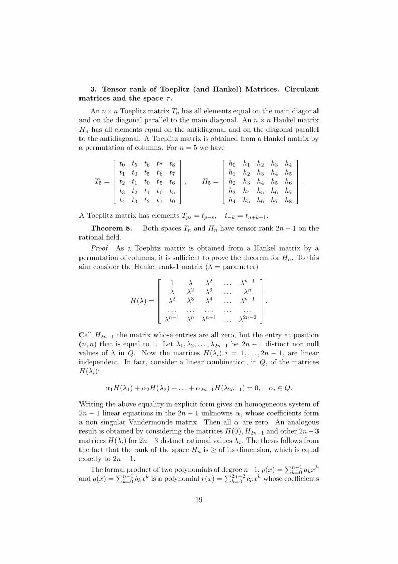
An n×n Toeplitz matrix Tn has all elements equal on the main diagonaland on the diagonal parallel to the main diagonal. An n× n Hankel matrixHn has all elements equal on the antidiagonal and on the diagonal parallelto the antidiagonal. A Toeplitz matrix is obtained from a Hankel matrix bya permutation of columns. For n = 5 we have

T5 =

t0 t5 t6 t7 t8t1 t0 t5 t6 t7t2 t1 t0 t5 t6t3 t2 t1 t0 t5t4 t3 t2 t1 t0

, H5 =

h0 h1 h2 h3 h4

h1 h2 h3 h4 h5

h2 h3 h4 h5 h6

h3 h4 h5 h6 h7

h4 h5 h6 h7 h8

.

A Toeplitz matrix has elements Tps = tp−s, t−k = tn+k−1.

Theorem 8. Both spaces Tn and Hn have tensor rank 2n− 1 on therational field.

Proof. As a Toeplitz matrix is obtained from a Hankel matrix by apermutation of columns, it is sufficient to prove the theorem for Hn. To thisaim consider the Hankel rank-1 matrix (λ = parameter)

H(λ) =

1 λ λ2 . . . λn−1

λ λ2 λ3 . . . λn

λ2 λ3 λ4 . . . λn+1

. . . . . . . . . . . . . . .λn−1 λn λn+1 . . . λ2n−2

.

Call H2n−1 the matrix whose entries are all zero, but the entry at position(n, n) that is equal to 1. Let λ1, λ2, . . . , λ2n−1 be 2n − 1 distinct non nullvalues of λ in Q. Now the matrices H(λi), i = 1, . . . , 2n − 1, are linearindependent. In fact, consider a linear combination, in Q, of the matricesH(λi):

α1H(λ1) + α2H(λ2) + . . .+ α2n−1H(λ2n−1) = 0, αi ∈ Q.

Writing the above equality in explicit form gives an homogeneous system of2n − 1 linear equations in the 2n − 1 unknowns α, whose coefficients forma non singular Vandermonde matrix. Then all α are zero. An analogousresult is obtained by considering the matrices H(0), H2n−1 and other 2n− 3matrices H(λi) for 2n−3 distinct rational values λi. The thesis follows fromthe fact that the rank of the space Hn is ≥ of its dimension, which is equalexactly to 2n− 1.

The formal product of two polynomials of degree n−1, p(x) =∑n−1k=0 akx

k

and q(x) =∑n−1k=0 bkx

k is a polynomial r(x) =∑2n−2h=0 chx

h whose coefficients

19

ch are defined by a set of n bilinear forms fh(a,b) = aTMhb, h = 1, 2, . . . , n,where the Mh are n× n Hankel matrices. Then 2n− 1 non-scalar multipli-cations are sufficient and necessary to compute p(x)q(x).

Exercise 6. For n = 3, multiply two polynomials of degree n by mean-s of the optimal decomposition of the associated tensor. Consider the proofof the previous Theorem 8, choosing the tensor basisH(0), H(1), H(−1), H(2), H2n−1

and prove that the only significant scalar operation is a division by 3.

A special class of Toeplitz matrices are the well known algebra of n× ncirculant matrices, a space generated by the first n powers of the circulantpermutation matrix P whose first row is [0 1 0 . . . 0]. A 5 × 5 circulantmatrix and the correspondent P have the form

C5 =

a0 a1 a2 a3 a4

a4 a0 a1 a2 a3

a3 a4 a0 a1 a2

a2 a3 a4 a0 a1

a1 a2 a3 a4 a0

, P =

0 1 0 0 00 0 1 0 00 0 0 1 00 0 0 0 11 0 0 0 0

.

It is easy to prove the following equalities for a n × n circulant matrixCn (see also [5]):

Cn =n−1∑h=0

ahPh, P iP j =

n−1∑h=0

tijhPh, tijh = (P i)jh = (P j)ih.

Moreover, Cn = F ∗nDFn, with (Fn)ij = ω(i−1)(j−1), ω = ei2π/n. Inother words all n × n circulant matrices can be reduced to diagonal formby the Fourier matrix Fn. Then the multiplicative table tijh has the samestructure of the matrices P h, so the tensor tijh = (P i)jh, whose rk(tijh) isequal to n over the complex field, is the tensor associated to the discreteconvolution on n points, defined precisely, for n = 5, as the product ofCn by a vector b = [b0 b4 b3 b2 b1]T . In fact, the convolution product oftwo vectors a = [a0 a1 . . . an−1]T and b = [b0 b1 . . . bn−1]T is a vectorc := a ? b = [c0 c1 . . . cn−1]T whose component ch is given by

ch =n−1∑

i+jmod h

aibj .

The formal product of the polynomials p(x) and q(x) of degree n−1 is definedby the convolution of the two (2n − 1)-vectors a = [a0 a1 . . . an−1 0 . . . 0]T

and b = [b0 b1 . . . bn−1 . . . 0]T .

To compute c = a ? b the following equality, known as the ConvolutionTheorem, is usually exploited:

c = a ? b = F−1n [(Fna) · (Fnb)]

20

where · denotes the element by element vector multiplication. The Convolu-tion Theorem is a consequence of the eigenvector decomposition of circulantmatrices (verify that!), and the previous equality defines a bilinear programon C to compute a ? b. The total asymptotic complexity of this programdepends on the complexity of the FFT, which is O(nlog2n).

The following space, called space τ , is an algebra of n×n symmetric andpersymmetric matrices reduced to diagonal form by a unitary matrix withreal elements. In [8] and in [32] some interesting links of τ with symmetricToeplitz matrices have been discovered. We write here below a matrix ofthe algebra τ for n = 5:

τ5 =

t1 t2 t3 t4 t5t2 t1 + t3 t2 + t4 t3 + t5 t4t3 t2 + t4 t1 + t3 + t5 t2 + t4 t3t4 t3 + t5 t2 + t4 t1 + t3 t2t5 t4 t3 t2 t1

.

The space τ is defined, in general, by a cross-sum property: ti−1,j +ti+1,j = ti,j−1 + ti,j+1, with suitable “boundary conditions”. The eigenvec-tors are defined by uij = ( 2

n+1)1/2sin ijπn+1 , so τ = UDUH . The space τ is

generated in R by the non-derogatory matrix

H =

0 1 0 0 01 0 1 0 00 1 0 1 00 0 1 0 10 0 0 1 0

.

Both circulant and τ matrices can be exploited to define fast algorithms formatrix by vector product when the matrix has Toeplitz form. In fact, ageneral n × n Toeplitz matrix is a part of a circulant matrix of dimension2n, so the problem Tn×vector can be reduced to a problem C2n×vector, andthen to a number of FFT on 2n points, with only O(nlog2n) operations.Consider here below the case n = 3:

t0 t3 t4 0 t2 t1t1 t0 t3 t4 0 t2t2 t1 t0 t3 t4 00 t2 t1 t0 t3 t4t4 0 t2 t1 t0 t3t3 t4 0 t2 t1 t0

×

s0s1s2000

.

Notice that the previous decomposition of the tensor of Toeplitz or Han-kel matrices, stated in Theorem 8, is not optimal, on the real field, for sym-metric Toeplitz matrices. In fact, consider the following split of a general

21

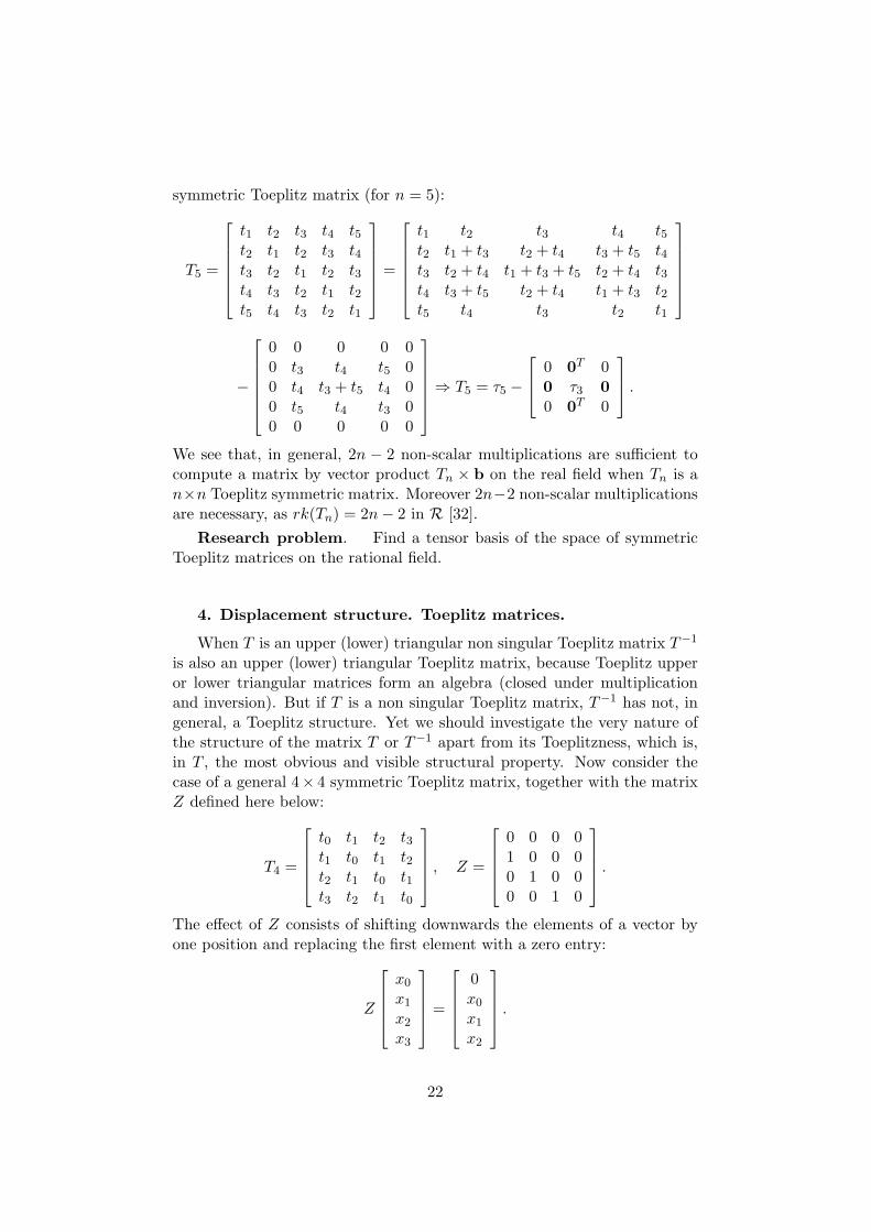
symmetric Toeplitz matrix (for n = 5):

T5 =

t1 t2 t3 t4 t5t2 t1 t2 t3 t4t3 t2 t1 t2 t3t4 t3 t2 t1 t2t5 t4 t3 t2 t1

=

t1 t2 t3 t4 t5t2 t1 + t3 t2 + t4 t3 + t5 t4t3 t2 + t4 t1 + t3 + t5 t2 + t4 t3t4 t3 + t5 t2 + t4 t1 + t3 t2t5 t4 t3 t2 t1

−

0 0 0 0 00 t3 t4 t5 00 t4 t3 + t5 t4 00 t5 t4 t3 00 0 0 0 0

⇒ T5 = τ5 −

0 0T 00 τ3 00 0T 0

.We see that, in general, 2n − 2 non-scalar multiplications are sufficient tocompute a matrix by vector product Tn × b on the real field when Tn is an×n Toeplitz symmetric matrix. Moreover 2n−2 non-scalar multiplicationsare necessary, as rk(Tn) = 2n− 2 in R [32].

Research problem. Find a tensor basis of the space of symmetricToeplitz matrices on the rational field.

4. Displacement structure. Toeplitz matrices.

When T is an upper (lower) triangular non singular Toeplitz matrix T−1

is also an upper (lower) triangular Toeplitz matrix, because Toeplitz upperor lower triangular matrices form an algebra (closed under multiplicationand inversion). But if T is a non singular Toeplitz matrix, T−1 has not, ingeneral, a Toeplitz structure. Yet we should investigate the very nature ofthe structure of the matrix T or T−1 apart from its Toeplitzness, which is,in T , the most obvious and visible structural property. Now consider thecase of a general 4× 4 symmetric Toeplitz matrix, together with the matrixZ defined here below:

T4 =

t0 t1 t2 t3t1 t0 t1 t2t2 t1 t0 t1t3 t2 t1 t0

, Z =

0 0 0 01 0 0 00 1 0 00 0 1 0

.The effect of Z consists of shifting downwards the elements of a vector byone position and replacing the first element with a zero entry:

Z

x0

x1

x2

x3

=

0x0

x1

x2

.

22

Now let T a Toeplitz matrix and define the operator ∇T as follows:

∇T := T − ZTZT = T −

0 0 0 00 t0 t1 t20 t1 t0 t10 t2 t1 t0

=

t0 t1 t2 t3t1 0 0 0t2 0 0 0t3 0 0 0

We have (for t0 = 1)

∇T = GJGT , G =

1 0t1 t1t2 t2t3 t3

, J =

[1 00 −1

], rk(GJGT ) = 2.

Notice that ∇T is symmetric when T is symmetric, so the eigenvalues of∇T are real. Moreover the two diagonal elements of J indicate that ∇T hasone eigenvalue positive and the other negative.The same operator ∇ can be applied to a general Hermitian matrix. In factlet, for an Hermitian matrix R,

∇R = R− ZRZH .

The matrix ZRZH corresponds to shifting R downwards along the maindiagonal by one position, which explains the name displacement for ∇R. If∇R has low rank, say r << n, then R is said to be structured with respectto the displacement defined by the operator ∇R, and r is referred as thedisplacement rank of R [20]. The matrix ∇R = R − ZRZH is Hermitian,its eigenvalues are real and we can define the displacement inertia of R asthe pair (p, q), where p and q are the number of the positive and negativeeigenvalues, respectively. The displacement rank r is equal precisely to p+qand then

∇R = R− ZRZH = GJGH , J = (Ip ⊕−Iq)

where J and G have dimensions r × r and n × r, respectively. In [20] thepair G, J is called a generator of R. In fact it contains all informationregarding R, that is the information on the structure allowing to reduce thespace for representing R and the useful information on the complexity of amatrix by vector product Ry. It is easy to prove that the only solution ofthe above equation is

R =n−1∑i=0

ZiGJGH(ZH)i.

In fact, let

R = GJGH + ZGJGHZH + Z2GJGH(ZH)2 + . . .+ Zn−1GJGH(ZH)n−1.

23

Now multiply on the left by Z and on the right by ZH . As Z is nilpotent,i.e. Zn = 0, we have

ZRZH = ZGJGHZH + Z2GJGH(ZH)2 + . . .+ Zn−1GJGH(ZH)n−1.

Then subtract term by term the last two equalities so to obtain, eventually,

R− ZRZH = GJGH .

IfG = [x0x1 . . .xp−1y0y1 . . .yq−1],

then we can rewrite the equality R =∑n−1i=0 Z

iGJGH(ZH)i in the form

R =p−1∑i=0

L(xi)LH(xi)−q−1∑i=0

L(yi)LH(yi), (5)

where

L(z) =

z0 0 . . . . . . 0z1 z0 0 . . . 0. . . . . . . . . . . . . . .zn−2 . . . . . . z0 0zn−1 . . . . . . z1 z0

.

Exercise 7. Prove that (5) is identical to the equalityR =∑n−1i=0 Z

iGJGH(ZH)i.

A general result concerning matrices with displacement structure statesthat the displacement inertia of a matrix R is in some way inherited by itsinverse. More precisely, we have the following

Theorem 9.[20] The displacement inertia of a Hermitian non singularmatrix R with respect to R − ZRZH is equal to the displacement inertiaof its inverse with respect to R−1 − ZHR−1Z, i.e. Inertia(R − ZRZH) =Inertia(R−1 − ZHR−1Z).

Proof. The theorem follows from the two identities, exploiting the Schurcomplements of R,[

R ZZH R−1

]=

[I 0

ZHR−1 I

] [R 00 R−1 − ZHR−1Z

] [I 0

ZHR−1 I

]Hand [

R ZZH R−1

]=

[I ZR0 I

] [R− ZRZH 0

0 R−1

] [I ZR0 I

]H,

The matrices R−ZRZH and R−1−ZHR−1Z are called Schur complements.As in general Inertia(ABAH) = Inertia(B) (Sylvester’s theorem: congruencetransformations preserve Inertia), the two matrices[

R 00 R−1 − ZHR−1Z

],

[R− ZRZH 0

0 R−1

]

24

have the same Inertia. This implies the final identity Inertia(R−ZRZH) =Inertia(R−1 − ZHR−1Z).

Exercise 8. Find (possibly in the matrix literature) a proof of theSylvester’s theorem: congruence transformations preserve Inertia.

A consequence of the above theorem is concerned with the Toeplitz ma-trices: the inverse of a non singular symmetric Toeplitz matrix T has thesame displacement Inertia of T . In fact Inertia(T − ZTZH) = (1, 1) =Inertia(T−1 − ZHT−1Z) = Inertia(T−1 − ZT−1ZH), because

IT I = T, IT−1I = T−1, IZH I = Z,

where I is the reverse identity matrix with ones on the antidiagonal andzeros elsewhere. Then we have precisely, for a pair of vectors x,y,

T−1 − ZT−1ZH = xxh − yyH =[

x y] [

1 00 −1

] [xH

yH

],

andT−1 = L(x)L(x)H − L(y)L(y)H ,

which is the celebrated formula of Gohberg-Semencul. By this formula thematrix-vector product T−1z can be computed, as the product Tz, througha small number of FFT, and then in only O(nlog2n) arithmetic operations.Thus iterative solvers for Toeplitz systems may be quite competitive becauseof a fast matrix by vector procedure with a small number of fast transforms.Notice that the result of Theorem 9 does not depend on the special form ofthe matrix Z and so the matrix Z could be replaced by a general matrix Ω:the displacement inertia of an Hermitian non singular matrix R with respectto R−ΩRΩH is equal to the displacement inertia of its inverse with respectto R−1 − ΩHR−1Ω.

References

1. Ammar, Gader, A variant of the Gohberg-Semencul formula involv-ing circulant matrices, SIAM Journal Matrix Analysis and Applications,12(1991), pp. 534-540

2. T.M. Apostol, Introduction to Analytic Number Theory, Springer,New York, 1976.

3. E.G. Belaga, Evaluation of polynomials of one variable with prelim-inary processing of coefficients, in A.A, Lyapunov, ed., Problems of Cyber-netics, Pergamon Press, 5(1961), pp. 1-13.

4. R. Bevilacqua, M. Capovani, Proprieta delle matrici a banda adelementi ed a blocchi, Bollettino U.M.I. (5) 13-B (1976), 844-861.

25

5. R. Bevilacqua, C. Di Fiore, P. Zellini, h-space Structure in MatrixDisplacement Formulas, Calcolo, 33(1996), pp. 11-35.

6. R. Bevilacqua, P. Zellini, Closure, Commutativity and Minimal Com-plexity of Some Spaces of Matrices, Linear and Multilinear Algebra, 25(1989),pp. 1-25.

7. D. Bini, M. Capovani, G. Lotti, F. Romani, Complessita numerica,Boringhieri, Torino, 1981.

8. D. Bini, M. Capovani, Spectral and Computational Properties of BandSymmetric Toeplitz Matrices, Linear Algebra and its Applications, 99-126

9. A. Borodin, I. Munro, The computational Complexity of Algebraicand Numeric Problems, Elsevier, New York, 1975.

10. P. Burgisser, M. Clausen, M.Amin Shokrollahi, Algebraic ComplexityTheory, Springer, Berlin, 1997.

11. M. Capovani, Sulla determinazione dell’inversa delle matrici tridiag-onali a blocchi, Calcolo, 7(1970), 295-303.

12. M. Capovani, Su alcune proprieta delle matrici tridiagonali e penta-diagonali, Calcolo, 8(1971), 149-159.

13. G.J. Chaitin, Information-Theoretic Limitations of Formal Systems,Journal of the ACM, 21(1974), 403-424.

14. C. Di Fiore, P. Zellini, Matrix Decompositions using DisplacementRank and Classes of Commutative Matrix Algebras, Linear Algebra and itsApplications, 229(1995), 49-99.

15. D. Fasino, L. Gemignani, Structural and Computational Propertiesof Possibly Singular Semiseparable Matrices, Linear Algebra and its Appli-cations, 340(2002), 183-198.

16. C.M. Fiduccia, Y. Zalcstein, Algebras having linear multiplicativecomplexities, Journal of the ACM, 24(1977), 311-331.

17. G.E. Forsythe, Today’s Computational Methods of Linear Algebra,SIAM Review, 9(1967), pp. 489-515.

18. P.D. Gader, Displacement Operator Based Decompositions of Ma-trices Using Circulants or Other Group Matrices, Linear Algebra and itsApplications, 139(1990), 111-131.

19. F.R. Gantmacher, M.G. Krein, Oszillationsmatrizen, Oszillationskerneund kleine Schwingungen mechanischer Systeme, Akademie Verlag, Berlin,1960.

20. T. Kailath, A.H. Sayed, Displacement Structure: Theory and Ap-plications, SIAM Review, 37(1995), 297-386.

21. A.N. Kolmogorov, Logical Basis for Information Theory and Proba-bility Theory, IEEE Transactions, IT-14(1968), 662-664.

22. J.B. Kruskal, Rank, Decomposition, and Uniqueness for 3-Way andN -Way Arrays, in R. Coppi, S. Bolasco (Editors), Multiway Data Analysis,Elsevier, New York, 1989, pp. 7-18.

23. J.C. Lafon, Base Tensorielle des Matrices de Hankel (ou de Toeplitz).Applications, Numerische Mathematik, 23(1975), 349-361.

26

24. J. Morgenstern, Note on a Lower Bound of the Linear Complexityof the Fast Fourier Transform, Journal of the ACM, 20(1973), 305-306.

25. T.S. Motzkin, Evaluation of polynomials and Evaluation of RationalFunctions, Bulletin of the American Mathematical Society, 61(1955), 163.

26. B. Parlett, Progress in Numerical Analysis, SIAM Review, 20(1978),443-456.

27. M.S. Paterson, Lectures at IAC, Roma, March 1974.28. J.E. Savage, An Algorithm for the Computation of Linear Forms,

SIAM Journal on Computing, 3(1974), 150-158.29. V. Strassen, Gaussian Elimination is Not Optimal, Numerische

Mathematik, 13(1969), 354-356.30. E. Tyrtyshnikov, Mosaic-Skeleton Approximations, Calcolo, 33(1996),

pp. 47-57.31. S. Winograd, On the Number of Multiplications Necessary to Com-

pute Certain Functions, Communications on Pure and Applied Mathematics,23(1970), 165-179.

32. P. Zellini, On the Optimal Computation of a Set of Symmetric andPersymmetric Bilinear Forms, Linear Algebra and its Applications, 23(1979),101-119.

33. P. Zellini, Optimal Bounds for Solving Tridiagonal Systems withPreconditioning, SIAM Journal on Computing, 17(1988), 1036-1043.

27