on a class of nonlocal wave equations from …
TRANSCRIPT
ON A CLASS OF NONLOCAL WAVE EQUATIONSFROM APPLICATIONS
HORST REINHARD BEYER∗, BURAK AKSOYLU† , AND FATIH CELIKER‡
September 29, 2014
Abstract. We study equations from the area of peridynamics, which is an extension of elasticity.The governing equations form a system of nonlocal wave equations. Its governing operator is foundto be a bounded, linear and self-adjoint operator on a Hilbert space. We study the well-posednessand stability of the associated initial value problem. We solve the initial value problem by applyingthe functional calculus of the governing operator. In addition, we give a series representation of thesolution in terms of spherical Bessel functions. For the case of scalar valued functions, the governingoperator turns out as functions of the Laplace operator. This result enables the comparison ofperidynamic solutions to those of classical elasticity as well as the introduction of local boundaryconditions into the nonlocal theory. The latter is studied in a companion paper.
Key words. Nonlocal wave equation, nonlocal operators, peridynamics, elasticity, operatortheory.
AMS subject classifications. 47G10, 35L05, 74B99
1. Motivation. Classical elasticity has been successful in characterizing andmeasuring the resistance of materials to crack growth. On the other hand, peridy-namics (PD), a nonlocal extension of continuum mechanics developed by Silling [63],is capable of quantitatively predicting the dynamics of propagating cracks, includ-ing bifurcation. Its effectiveness has been established in sophisticated applicationssuch as Kalthoff-Winkler experiments of the fracture of a steel plate with notches[36, 64], fracture and failure of composites, nanofiber networks, and polycrystal frac-ture [38, 52, 66, 65]. Further applications are in the context of multiscale modeling,where PD has been shown to be an upscaling of molecular dynamics [60, 62] and hasbeen demonstrated as a viable multiscale material model for length scales rangingfrom molecular dynamics to classical elasticity [10]. Also see other related engineer-ing applications [14, 37, 39, 54, 53], the review and news articles [16, 21, 43] for acomprehensive discussion, and the recent book [45].
We study a class of nonlocal wave equations. The driving application is PD.The same operator is also employed in nonlocal diffusion [9, 16, 59]. Similar classes ofoperators are used in numerous applications such as population models [13, 50], imageprocessing [31, 40], particle systems [12], phase transition [8, 7], and coagulation [30].In addition, we witness a major effort to meet the need for mathematical theory for
∗Department of Mathematics, TOBB University of Economics and Technology, Ankara, 06560,Turkey & Instituto Tecnologico Superior de Uruapan, Carr. Uruapan-Carapan No. 5555, Col. LaBasilia, Uruapan, Michoacan. Mexico & Theoretical Astrophysics, IAAT, Eberhard Karls Universityof Tubingen, Tubingen 72076, Germany, [email protected].†Department of Mathematics, TOBB University of Economics and Technology, Ankara, 06560,
Turkey & Department of Mathematics and Statistics, University of New Mexico, Albuquerque, NM87131, USA, [email protected]. This work was supported in part by National Science FoundationDMS 1016190 grant, European Commission Marie Curie Career Integration Grant 293978, and Scien-tific and Technological Research Council of Turkey (TUBITAK) TBAG 112T240 and MAG 112M891grants. Research visit of Horst R. Beyer was supported in part by TUBITAK 2221 Fellowship forVisiting Scientist Program. Sabbatical visit of Fatih Celiker was supported in part by TUBITAK2221 Fellowship for Scientist on Sabbatical Leave Program.‡Department of Mathematics, Wayne State University, 656 W. Kirby, Detroit, MI 48202, USA,
[email protected]. This work was supported in part by National Science Foundation DMS1115280 grant.
1
arX
iv:1
409.
7525
v1 [
mat
h-ph
] 2
6 Se
p 20
14

2 Horst R. Beyer and Burak Aksoylu and Fatih Celiker
PD applications and related nonlocal problems addressing, for instance, conditioninganalysis, domain decomposition and variational theory [3, 4, 5], volume constraints[16, 18, 17], nonlinearity [24, 25, 26, 44], discretization [1, 5, 29, 68], numerical methods[15, 19, 22, 58], and various other aspects [6, 20, 23, 27, 28, 32, 33, 41, 42, 46, 47, 48,60, 61, 72].
It is part of the folklore in physics that the point particle model, which is the rootfor locality in physics, is the cause of unphysical singular behavior in the description ofthe underlying phenomena. This fact is a strong indication that, in the long run, thedevelopment of nonlocal theories is necessary for description of natural phenomena.Operator theory does not discern the locality or nonlocality of the governing operator.This is the strength of this approach. This article adds valuable tools to the arsenal ofmethods to analyze nonlocal problems, thereby, increasing structural understandingin the field.
The rest of the article is structured as follows. We start with a mathematicalintroduction in Section 1.1. In Section 2, we set the operator theory framework totreat the nonlocal wave equation. We prove basic properties of the solutions such aswell-posedness of the initial value problem and provide a representation of the solu-tions in terms of bounded functions of the governing operator. We study the stabilityof solutions and give conservation laws. In Section 3, in the vector-valued case, wenote that the governing operator becomes an operator matrix. The generality of op-erator theory allows a simple extension of the results established for the scalar-valuedfunctions to the vector-valued ones. We prove the boundedness of the entries of thegoverning operator matrix. The proof is natural due to operator theory again, becauseit relies on a well-known criterion for integral operators. We present a “diagonaliza-tion” of the matrix entries. This is accomplished by employing the unitary Fouriertransform and connecting the entries to maximal multiplication operators. We studythe spectral properties of the entries. Then, we reach to a notable result. Namely, weprove that the governing operator is a bounded function of the classical local operator.This has far reaching consequences. It enables the incorporation of local boundaryconditions into nonlocal theories, which is the subject of our companion paper [2].We introduce notion of strong resolvent convergence. This allows us to prove theconvergence of solutions of the governing equation to that of the classical solution.We give examples of sequences of micromoduli that are instance of this result. InSection 4, we consider the calculation of the solution of the wave equation. Sincethe governing operator is bounded, holomorphic functions of that operator can berepresented in form of power series in the operator. Then, we give a representation ofholomorphic functions, present in the solution of the initial value problem, utilizingthe fact that the governing operator is a sum of two commuting operators. We dis-cover that the corresponding power series can be given in terms of a series of Besselfunctions. In Section 5, we apply the representation in terms of Bessel functions tospecial Gaussian micromoduli and Gaussian data. We depict the resulting solutionsof peridynamic wave equation and compare to the classical solutions. We conclude inSection 6.
1.1. Mathematical Introduction. The formal system of linear peridy-namic wave equations in n-space dimensions [63, Eqn. 54] n ∈ N∗, is given by
ρ∂2u
∂t2(x, t) =
∫RnC(x′ − x) · (u(x′, t)− u(x, t)) dx′ + b(x, t) , (1.1)

Nonlocal Wave Equations 3
where “·” indicates matrix multiplication, or equivalently by the system
ρ∂2uj∂t2
(x, t) =
n∑k=1
∫RnCjk(x′ − x) · (uk(x′, t)− uk(x, t)) dx′ + bj(x, t) , (1.2)
where x ∈ Rn, t ∈ R, C : Rn → M(n × n,R) is the micromodulus tensor, assumedto be even and assuming values inside the subspace of symmetric matrices, ρ > 0is the mass density, b : Rn × R → Rn is the prescribed body force density, andu : Rn × R→ Rn is the displacement field.
For comparison, e.g., the corresponding wave equation in classical elasticity in1-space dimension is given by
ρ∂2u
∂t2= E
∂2u
∂x2+ b , (1.3)
where E > 0 is the so called “Young’s modulus,” and describing compression wavesin a rod.
If j, k ∈ {1, . . . , n} and Cjk ∈ L1(Rn), we can rewrite (1.2) as
ρ∂2uj∂t2
(x, t) = −n∑k=1
{[∫RnCjk(x′)dx′
]uk(x, t)− (Cjk ∗ uk(·, t))(x)
}+ bj(x, t) ,
(1.4)for all x ∈ Rn, t ∈ R and j ∈ {1, . . . , n} where ∗ denotes the convolution product.The system (1.4) is the starting point for a functional analytic interpretation, whichleads on a well-posed initial value problem. For this purpose, we use methods fromoperator theory; see, e.g., [11, 55].
2. Operator-Theoretic Treatment of Systems of Wave Equations.Analogous to the majority of evolution equations from classical and quantum physics,(1.4) can be treated with methods from operator theory, see, e.g., [11, 55] for sub-stantiation of this claim and [34] for applications of operator theory in engineering.More specifically, this system falls into the class of abstract linear wave equations fromTheorem 2.1. For the proof of this theorem see, e.g., [11, Thm. 2.2.1 and Cor. 2.2.2].Special cases of this theorem are proved in [35, 49] and [56, Vol. II]. Statements andproofs make use of the spectral theorems of (densely-defined, linear and) self-adjointoperators in Hilbert spaces, including the concept of functions of such operators, see,e.g., [56, Vol. I], or standard books on Functional Analysis, such as [57, 71]. Thesemethods are also used throughout the paper.
This section provides the basic properties of the solutions of abstract wave equa-tions of the form (2.1). Some of the subsequent results are scattered in the literature.Therefore, wherever necessary, we provide proofs. In particular, Theorem 2.1 givesthe well-posedness of the initial value problem for a class of abstract wave equations,conservation of energy and a representation of the solutions in terms of boundedfunctions of the governing operator. Corollary 2.2 and Theorem 2.3 are results onthe stability of the solutions, i.e., their growth for large times. Theorem 2.4 providesconservation laws induced by symmetries of the governing operator. Theorem 2.5provides special solutions of the associated class of inhomogeneous wave equations.Together with Theorem 2.1, these solutions provide the well-posedness of the initialvalue problem of the latter equations as well as a representation of the solutions interms of bounded functions of the governing operator.
Theorem 2.1. (Wave Equations) Let (X, 〈|〉) be some non-trivial complex
4 Horst R. Beyer and Burak Aksoylu and Fatih Celiker
Hilbert space. Furthermore, let A : D(A) → X be some densely-defined, linear,semibounded self-adjoint operator in X with spectrum σ(A). Finally, let ξ, η ∈ D(A).
(i) Then there is a unique twice continuously differentiable map u : R → Xassuming values in D(A) and satisfying
u ′′(t) = −Au(t) (2.1)
for all t ∈ R as well as
u(0) = ξ , u ′(0) = η .
(ii) For this u, the corresponding energy function Eu : R→ R, defined by
Eu(t) :=1
2
(〈u ′(t)|u ′(t)〉+ 〈u(t)|Au(t)〉
)for all t ∈ R, is constant.
(iii) Moreover, this u is given by
u(t) =
[cos(t√ )∣∣∣∣
σ(A)
](A)ξ +
[sin(t√ )√
∣∣∣∣σ(A)
](A)η (2.2)
for all t ∈ R, where
cos(t√
) andsin(t√
)√
denote the unique extensions of cos(t√
) and sin(t√
)/√
, respectively,to entire holomorphic functions.
Moreover, if A is positive, the solutions of (2.1) are stable, i.e., there are nosolutions that are growing exponentially in the norm.
Corollary 2.2. (Stability of Solutions) If A is positive, then
‖u(t)‖ 6 ‖ξ‖+ |t| · ‖η‖
for every t ∈ R.Proof. The statement follows from Theorem 2.1 (iii), since, from an application
of the spectral theorem of densely-defined, linear and self-adjoint operators in Hilbertspaces, it follows that the operator norms of the operators in (2.2) satisfy∥∥∥∥
[cos(t√ )∣∣∣∣
σ(A)
](A)
∥∥∥∥ 6 1 ,
∥∥∥∥[
sin(t√ )√
∣∣∣∣σ(A)
](A)
∥∥∥∥ 6 t ,
for every t ∈ R.On the other hand, if A is strictly negative, there are solutions of (2.1) that are
growing exponentially in the norm. The corresponding theorem is not readily foundin the literature. For the convenience of the reader, we give a proof in the Appendix.
Theorem 2.3. (Instability of Solutions) If (X, 〈|〉), A : D(A)→ X, σ(A) areas in Theorem 2.1 and, in addition, A is such that
σ(A) ∩ (−∞, 0) 6= ∅ ,
Nonlocal Wave Equations 5
then there is a twice continuously differentiable map assuming values in D(A) andsatisfying
u ′′(t) = −Au(t)
for all t ∈ R with exponentially growing norm.Proof. See the Appendix.The following Theorem 2.4 can be considered a form of Noether’s Theorem for
the solutions of (2.1). For the convenience of the reader, we provide a proof in theAppendix.
Theorem 2.4. (Conservation Laws Induced by Symmetries) Let u, v :R → X be twice continuously differentiable map assuming values in D(A) and satis-fying
u ′′(t) = −Au(t) , v ′′(t) = −Av(t)
for all t ∈ R. Then the following holds.(i) Then ju,v : R→ C, defined by
ju,v(t) := 〈u(t)|v′(t)〉 − 〈u′(t)|v(t)〉
for every t ∈ R, is constant.(ii) If B ∈ L(X,X) commutes with A, i.e., is such that A ◦B ⊃ B ◦A, then
ju,B(t) := 〈u(t)|Bu′(t)〉 − 〈u′(t)|Bu(t)〉
for every t ∈ R, is constant.(iii) If B is a densely-defined, linear self-adjoint operator in X that commutes
with A, i.e., is such that every member of its associated spectral family com-mutes with every member of the spectral family that is associated to A, andu(0), u′(0) ∈ D(A) ∩D(B), then Ran(u),Ran(u′) ⊂ D(A) ∩D(B) and
ju,B(t) := 〈u(t)|Bu′(t)〉 − 〈u′(t)|Bu(t)〉
for every t ∈ R, is constant.Proof. See the Appendix.Duhamel’s principle leads to a solution of (2.1) for vanishing data, the proof of
the well-posedness and a representation of the solutions of the initial value problemof the inhomogeneous equation,
u ′′(t) = −Au(t) + b(t) ,
t ∈ R. For simplicity, the corresponding subsequent Theorem 2.5 assumes that A is inaddition positive, which is the most relevant case for applications because otherwisethere are exponentially growing solutions, indicating that the system is unstable; seeTheorem 2.3. The same statement is true if σ(A) is only bounded from below. Onthe other hand, Theorem 2.5 can also be obtained by application of the correspondingwell-known more general theorem for strongly continuous semigroups; see, e.g., [11,Thm. 4.6.2]. We give a direct proof of Theorem 2.5 in the Appendix, which does notrely on methods from the theory of strongly continuous semigroups. For the definitionof weak integration; see, e.g., [11, Sec. 3.2].
Theorem 2.5. (Solutions of Inhomogeneous Wave Equations) Let (X, 〈|〉),A : D(A) → X, σ(A) be as in Theorem 2.1 and, in addition, A be positive. Finally,

6 Horst R. Beyer and Burak Aksoylu and Fatih Celiker
let f : R→ X be a continuous map, assuming values in D(A2) such that Af , A2f arecontinuous. Then, v : R→ X, for every t ∈ R defined by
v(t) :=
∫It
[sin((t− τ)
√ )√
∣∣∣∣σ(A)
](A)f(τ) dτ ,
where∫
denotes weak integration in X,
It :=
{[0, t] if t > 0
[t, 0] if t < 0,
is twice continuously differentiable, assumes values in D(A), is such that
v(0) = v′(0) = 0 ,
and
v ′′(t) +Av(t) = f(t), t ∈ R.
Proof. See the Appendix.
3. The Governing Operator and Properties. The standard data spacefor the classical wave equation is a L2-space with constant weight, on a non-emptyopen subset of Rn, n ∈ N∗, for instance, L2
C(R) for a bar of infinite extension in 1-space dimension. It turns out that the classical data spaces are suitable also as dataspaces for peridynamics, for instance, again L2
C(R) for a bar of infinite extension in1-space dimension, composed of a “linear peridynamic material.” This simplifies thediscussion of the convergence of peridynamic solutions to classical solutions.
In the following, we represent (1.4) in form of (2.1), where the governing oper-ator A is an “operator matrix,” consisting of sums of multiples of the identity andconvolution operators, as indicated in (1.4). These matrix entries will turn out to bepairwise commuting. The following remark provides some known relevant informa-tion on operator matrices of bounded operators. On the other hand, we avoid explicitmatrix notation.
Remark 3.1. (Operator Matrices) If K ∈ {R,C}, (X, 〈 | 〉) a non-trivial K-Hilbert space, (Ajk)j,k∈{1,...,n} a family of elements of L(X,X).
(i) Then by
A(ξ1, . . . , ξn) :=
(n∑k=1
A1kξk, . . . ,
n∑k=1
Ankξk
)
for every (ξ1, . . . , ξn) ∈ Xn, there is defined a bounded linear operator withadjoint A∗ given by
A∗(ξ1, . . . , ξn) =
(n∑k=1
A∗k1ξk, . . . ,
n∑k=1
A∗knξk
)
for every (ξ1, . . . , ξn) ∈ Xn.

Nonlocal Wave Equations 7
(ii) If the members of (Ajk)j,k∈{1,...,n} are pairwise commuting, then A is bijectiveif and only if det(A) is bijective, where
det(A) :=∑σ∈Sn
sign(σ)A1σ(1) · · ·Anσ(n) ,
Sn denotes the set of permutations of {1, . . . , n},
sign(σ) :=
n∏i,j=1,i<j
sign(σ(j)− σ(i))
for all σ ∈ Sn and sign denotes the signum function.The basic properties of the entries of the operator matrix are given in the following
lemma. In fact, these operators turn out to be bounded linear operators on L2C(Rn).
Hence, the boundedness and self-adjointness of A follows from those of AC . Theboundedness of A has been shown in [23, 28, 72] for special class of kernel functions.We generalize the result to kernel functions that are in L1(Rn) by utilizing a well-known criterion for integral operators; see, e.g., Corollary to [70, Thm. 6.24].
Lemma 3.2. (Matrix Entries) Let n ∈ N∗, ρ > 0 and C ∈ L1(Rn) be even.Then,
ACf :=1
ρ
[(∫RnC dvn
).f − C ∗ f
], (3.1)
for every f ∈ L2C(Rn), where ∗ denotes the convolution product, there is defined a
self-adjoint bounded linear operator on L2C(Rn) with operator norm ‖AC‖ satisfying
‖AC‖ 61
ρ
( ∣∣∣∣ ∫RC dvn
∣∣∣∣+ ‖C‖1)
62‖C‖1ρ
. (3.2)
Proof. For this purpose, we define the projections p1, p2 : R2n → Rn by
p1(x1, . . . , xn, y1, . . . , yn) := (x1, . . . , xn) , p2(x1, . . . , xn, y1, . . . , yn) := (y1, . . . , yn)
for all (x1, . . . , xn, y1, . . . , yn) ∈ R2n, and K := C ◦(p1−p2). Taking into account thatC is in particular measurable, as a consequence of the theory of Lebesgue integration,K is measurable. Also, since C is even, K is symmetric. Furthermore, for everyx ∈ Rn and y ∈ Rn
K(x, ·) = C(x− ·) = C(· − x) , K(·, y) = C(· − y) ∈ L1(Rn)
and
‖K(x, ·)‖1 = ‖K(·, y)‖1 = ‖C‖1 .
Hence according to a well-known criterion for integral operators on L2-spaces, see,e.g., Corollary to [70, Thm. 6.24], to K there corresponds a self-adjoint boundedlinear integral operator Int(K) on L2
C(Rn) with operator norm 6 ‖C‖1 and for almostall x given by
[Int(K)f ](x) =
∫RnK(x, ·) · f dvn =
∫RnC(x− ·) · f dvn = (C ∗ f)(x) .

8 Horst R. Beyer and Burak Aksoylu and Fatih Celiker
Hence by (3.1), there is given a self-adjoint bound linear operator AC with operatornorm ‖AC‖ satisfying (3.2).
For the study of the spectral properties of the matrix entries, needed for the appli-cation of the results from Section 2, we use Fourier transformations. This step parallelsthe common procedure for constant coefficient differential operators on Rn, n ∈ N∗.With the help of the unitary Fourier transform F2, Theorem 3.4 represents the matrixentries as maximal multiplication operators. This process can be viewed as a form of“diagonalization” of the entries. Also, since bounded maximal multiplication opera-tors commute, the entries commute pairwise. The spectra of maximal multiplicationoperators are well understood, leading to Corollary 3.5. Also, the functional calcu-lus which is associated to maximal multiplication operators is known and allows theconstruction of the functional calculi of the entries. The latter is used in the proof ofTheorem 3.6 which proves that matrix entries corresponding to spherically symmetricmicromoduli are functions of the Laplace operator.
Assumption 3.3. In the following, for n ∈ N∗, F2 denotes the unitary Fouriertransformation on L2
C(Rn) which, for every rapidly decreasing test function f ∈SC(R), is defined by
(F2f)(k) :=1
(2π)n/2
∫Rne−ik·idRn f dvn, k ∈ Rn.
Also, we denote by F1 the map from L1C(Rn) to C∞(Rn,C), the space of continuous
functions on Rn vanishing at infinity, which for every f ∈ L1C(Rn), is defined by
(F1f)(k) :=
∫Rne−ik·idRn f dvn, k ∈ Rn.
Theorem 3.4. (Fourier Transforms of the Entries) Let
T 1ρ [(F1C)(0)−F1C]
denote the maximal multiplication operator by the bounded continuous function
1
ρ[(F1C)(0)− F1C]
on L2C(Rn). Then
F2 ◦AC ◦ F−12 = T 1
ρ [(F1C)(0)−F1C] .
Proof. The statement is a consequence of the fact that
[F2 ◦ Int(K)]f = [TF1C ◦ F2]f
for every f ∈ L2C(Rn), where K and Int(K) are defined as in Lemma 3.2 and where
TF1C denotes the maximal multiplication operator on L2C(Rn) by the bounded contin-
uous function F1C. For the proof of this fact, we note that for every L1C(Rn)∩L2
C(Rn)
[F2 ◦ Int(K)]f = F2(C ∗ f) =1
(2π)n/2.F1(C ∗ f) =
1
(2π)n/2.(F1C)(F1f)

Nonlocal Wave Equations 9
= (F1C)(F2f) = [TF1C ◦ F2]f .
Hence, since L1C(Rn) ∩ L2
C(Rn) is dense in L2C(Rn), the bounded linear operators
F2 ◦ Int(K) and TF1C ◦ F2 coincide on a dense subspace of L2C(Rn) and therefore
coincide on the whole of L2C(Rn).
We give the spectrum and point spectrum of AC .Corollary 3.5. (Spectral Properties of the Entries)
σ(AC) = Ran1
ρ.[(F1C)(0)− F1C] ,
σp(AC) =
{λ ∈ R :
{k ∈ R :
1
ρ.[(F1C)(0)− (F1C)(k)] = λ
}is no Lebesgue null set
},
where the overline denotes the closure in R. Finally, for every λ ∈ σ(AC), AC − λ isnot surjective.
Proof. Let T 1ρ [(F1C)(0)−F1C] denote maximal multiplication operator by the bounded
continuous function 1ρ [(F1C)(0)− F1C] on L2
C(Rn). Since F2 is an unitary operator
F2 ◦AC ◦ F−12 = T 1
ρ [(F1C)(0)−F1C] ,
where the spectra and the point spectra of AC and T 1ρ [(F1C)(0)−F1C] coincide, re-
spectively. Hence it follows from the properties of maximal multiplication operatorsthat
σ(AC) =
{λ ∈ R :
(1
ρ[(F1C)(0)− F1C]
)−1
(Uc(λ))
is no Lebesgue null set for every c > 0
},
σp(AC) =
{λ ∈ R :
(1
ρ[(F1C)(0)− F1C]
)−1
(λ)
is no Lebesgue null set
}.
Since R \ Ran 1ρ .[(F1C)(0)− F1C] is open, for λ ∈ R \ Ran 1
ρ .[(F1C)(0)− F1C], thereis ε > 0 such that
{k ∈ R :1
ρ.[(F1C)(0)− (F1C)(k) ∈ (λ− ε, λ+ ε)}
is empty, and hence λ /∈ σ(AC). On the other hand, since 1ρ [(F1C)(0) − F1C] is
continuous, for λ ∈ Ran 1ρ .[(F1C)(0)− F1C] and c > 0,(
1
ρ[(F1C)(0)− F1C]
)−1
(Uc(λ))
is non-empty and open, hence no Lebesgue null set and λ ∈ σ(A). Since σ(AC) isclosed, it follows that
σ(AC) = Ran1
ρ.[(F1C)(0)− F1C] .

10 Horst R. Beyer and Burak Aksoylu and Fatih Celiker
Finally, for λ ∈ R, since
F2 ◦ (AC − λ) ◦ F−12 = T 1
ρ [(F1C)(0)−F1C]−λ
it follows that AC−λ is surjective if and only if T 1ρ [(F1C)(0)−F1C]−λ is surjective. From
the properties of maximal multiplication operators, it follows that the latter operatoris surjective if and only if it is bijective and hence if and only if λ ∈ R \ σ(AC).
The notable result we obtained is that the governing operator AC of the peridy-namic wave equation is a bounded function of the classical governing operator, presentin (1.3). This observation has far reaching consequences. It enables the comparisonof peridynamic solutions to those of classical elasticity. In the past, only the conver-gence of the peridynamic operator to the classical operator has been discussed; see[4, 5, 41, 72]. More important for applications is the corresponding convergence ofsolutions. The tool that has been developed for this purpose is the notion of strongresolvent convergence used in Theorem 3.10.
The other remarkable implication is the definition of peridynamic-type operatorson bounded domains as functions of the corresponding classical operator. Since theclassical operator is defined through local boundary conditions, the functions inheritthis knowledge. This observation opens a gateway to incorporate local boundaryconditions to nonlocal theories, which has vital implications for numerical treatmentof nonlocal problems. This is the subject of our companion paper [2].
Theorem 3.6. (A Representation of Matrix Entries Corresponding toSpherically Symmetric Micromoduli as Functions of the Laplace Opera-tor) Let n ∈ N∗, Ln be the closure of the positive symmetric, essentially self-adjointoperator in L2
C(Rn), given by(C∞0 (Rn,C)→ L2
C(Rn) , f 7→ −Eρ4f),
where ρ > 0 and E > 0. Furthermore, if n > 1, in addition, let C be sphericallysymmetric, i.e., such that
C ◦R = C ,
for every R ∈ SO(n), where SO(n) denotes the map of group of special orthogonaltransformations on Rn. Then
AC =
{1
ρ[(F1C)(0)− F1C] ◦ ι
}(Ln) ,
where ι : [0,∞)→ Rn is defined by
ι(s) :=
(√ρ
Es
).e1 ,
for every s > 0 and e1, . . . , en denotes the canonical basis of Rn.
Proof. First, we note that
F2 ◦ Ln ◦ F−12 = TE
ρ | |2,

Nonlocal Wave Equations 11
where TEρ | |2
denotes the maximal multiplication operator in L2C(Rn) by the function
Eρ | |
2. In particular, this implies that the spectrum of Ln, σ(Ln), is given by [0,∞)
and for every g ∈ UsC([0,∞)) ∗ that
g(Ln) = F−12 ◦ Tg◦(Eρ | |2) ◦ F2 ,
where Tg◦(Eρ | |2)denotes the maximal multiplication operator on L2
C(Rn) by the func-
tion
g ◦(E
ρ| |2).
Furthermore, we note that (F1C)(0) − F1C ∈ BC(Rn,R), where BC(Rn,R) is thespace of real-valued bounded continuous on Rn, and that (F1C)(0) − F1C is even,since for every k ∈ Rn
(F1C)(−k) =
∫Rneik·idRnC dvn =
∫Rne−ik·idRn [C ◦ (−idRn)] dvn
=
∫Rne−ik·idRnC dvn = (F1C)(k) ,
(F1C)(k) =1
2
[∫Rne−ik·idRnC dvn +
∫Rneik·idRnC dvn
]=
∫Rn
cos(k · idRn)C dvn ,
(F1C)(0)− (F1C)(k) =
∫Rn
[1− cos(k · idRn)]C dvn = 2
∫Rn
sin2
(k
2· idRn
)C dvn .
Furthermore for n > 1, we note that
(F1C)(R(k)) =
∫Rne−iR(k)·idRnC dvn =
∫Rne−iR(k)·R (C ◦R) dvn
=
∫Rne−ik·idRn (C ◦R) dvn =
∫Rne−ik·idRnC dvn = (F1C)(k)
for every R ∈ SO(n) and k ∈ Rn and hence that
(F1C)(k) = (F1C)(|k|.e1)
for every k ∈ Rn. In particular,
1
ρ[(F1C)(0)− F1C] ◦ ι ∈ UsR([0,∞))
and {1
ρ[(F1C)(0)− F1C] ◦ ι
}(Ln) = F−1
2 ◦ T{ 1ρ [(F1C)(0)−F1C]◦ι
}◦(Eρ | |2)
◦ F2
= F−12 ◦ T 1
ρ [(F1C)(0)−F1C]◦( | |.e1) ◦ F2 = F−12 ◦ T 1
ρ [(F1C)(0)−F1C] ◦ F2 = AC .
∗UsC([0,∞)) denotes the space of bounded complex-valued functions on [0,∞) that are strongly
measurable in the sense that they are everywhere [0,∞) limit of a sequence of step functions.

12 Horst R. Beyer and Burak Aksoylu and Fatih Celiker
Lemma 3.7 gives conditions for the convergence of bounded functions of a self-adjoint operator to converge to that operator, which implies strong resolvent con-vergence and also the strong convergence of the same bounded continuous functionof each member of the sequence against that bounded continuous function of theself-adjoint operator; see Theorem 3.10.
Lemma 3.7. (Convergence of Bounded Functions of a Self-Adjoint Op-erator to that Operator) Let (X, 〈 | 〉) be a non-trivial complex Hilbert space andA : D(A) → X a densely-defined, linear and self-adjoint operator with spectrumσ(A). Furthermore, let f1, f2, . . . be a sequence in UsC(σ(A)) that is everywhere onσ(A) pointwise convergent to idσ(A), and for which there is M > 0 such that
|fν | 6M [(1 + | |)|σ(A)] (3.3)
for all ν ∈ R. Then
limν→∞
fν(A)ξ = Aξ , ξ ∈ D(A).
Proof. Let ξ ∈ D(A) and ψξ the corresponding spectral measure. Accordingto the spectral theorem for densely-defined, self-adjoint linear operators in Hilbertspaces, id2
R is ψξ-summable and
‖fµ(A)ξ − fν(A)ξ‖2 = ‖(fµ − fν)(A)ξ‖2
= 〈(fµ − fν)(A)ξ|(fµ − fν)(A)ξ〉 = 〈ξ||fµ − fν |2(A)ξ〉
=
∫σ(A)
|fµ − fν |2 dψξ = ‖fµ − fν‖22,ψξ = ‖fµ − idσ(A) + idσ(A) − fν‖22,ψξ
6(‖fµ − idσ(A)‖2,ψξ + ‖idσ(A) − fν‖2,ψξ
)2,
for µ, ν ∈ N∗. As a consequence of the pointwise convergence of f1, f2, . . . on σ(A) toidσ(A), (3.3) and Lebesgue’s dominated convergence theorem, it follows that
limµ→∞
‖fµ − idσ(A)‖2,ψξ = 0
and hence that f1(A)ξ, f2(A)ξ, . . . is a Cauchy sequence in X. Since (X, ‖ ‖) is inpar-ticular complete, the latter implies that f1(A)ξ, f2(A)ξ, . . . is convergent in (X, ‖ ‖).Furthermore,
〈ξ| limν→∞
fν(A)ξ〉 = limν→∞
〈ξ|fν(A)ξ〉 = limν→∞
∫σ(A)
fν dψξ
=
∫σ(A)
idσ(A) dψξ = 〈ξ|Aξ〉 ,
where again the pointwise convergence of f1, f2, . . . on σ(A) to idσ(A), (3.3), Lebesgue’sdominated convergence theorem and the spectral theorem for densely-defined, self-adjoint linear operators in Hilbert spaces has been applied. From the polarizationidentity for 〈 | 〉, it follows that
〈ξ| limν→∞
fν(A)η〉 = 〈ξ|Aη〉

Nonlocal Wave Equations 13
for all ξ, η ∈ D(A). Since D(A) is dense in X, the latter implies that
〈ξ| limν→∞
fν(A)η〉 = 〈ξ|Aη〉
for all ξ ∈ X, η ∈ D(A) and hence for every η ∈ D(A) that
limν→∞
fν(A)η = Aη .
Examples 3.8 and 3.9 provide sequences of micromoduli which satisfy the condi-tions of Lemma 3.7. Example 3.8 has also been treated in [48, 67] and Example 3.9has been treated in [48]. Example 3.11 applies Theorem 3.10 to the sequences of mi-cromoduli from Examples 3.8 and 3.9. As a consequence, for fixed data and t ∈ R, thesolutions of the initial value problem at time t corresponding to the members of eachsequence of micromoduli converge in L2
C(R) to the corresponding classical solution attime t.
Example 3.8. For every ν ∈ N∗, we define Cν ∈ L1(R) by
Cν := 3Eν3χ[− 1
ν, 1ν ]. (3.4)
For ν ∈ N∗
F1Cν = 6Eν3 sin(ν−1.idR)
idR,
where
sin(ν−1.idR)
idR
denotes the unique extension of sin(ν−1.idR)/idR to a continuous function on R. Fur-thermore, for ν ∈ N∗, λ > 0
1
ρ[(F1Cν)(0)− F1C] ◦ ι(λ) =
1
ρ[(F1Cν)(0)− F1Cν ]
(√ρ
Eλ
)=
6Eν2
ρ
[1− sin(ν−1.idR)
ν−1.idR
](√ρ
Eλ
)and k > 0
1− sin(k/ν)
k/ν= ν
∫ 1/ν
0
[1− cos(kx)] dx =
∫ 1
0
[1− cos(ku/ν)] du
=
∫ 1
0
[∫ k/ν
0
u sin(uy) dy
]du =
k
ν
∫ 1
0
[∫ 1
0
u sin(kuv/ν) dv
]du
=k2
ν2
∫[0,1]2
u2vsin(kuv/ν)
kuv/νdudv
and hence that
ν2
[1− sin(k/ν)
k/ν
]= k2
∫[0,1]2
u2vsin(kuv/ν)
kuv/νdudv .
14 Horst R. Beyer and Burak Aksoylu and Fatih Celiker
From the latter, we conclude with the help of Lebesgue’s dominated convergence theo-rem that
limν→∞
ν2
[1− sin(k/ν)
k/ν
]=k2
6
as well as that∣∣∣∣ν2
[1− sin(k/ν)
k/ν
] ∣∣∣∣ 6 k2
∫[0,1]2
u2v
∣∣∣∣ sin(kuv/ν)
kuv/ν
∣∣∣∣ dudv 6 k2
∫[0,1]2
u2v dudv =k2
6.
In particular, we conclude for λ > 0 that
limν→∞
1
ρ[(F1Cν)(0)− F1C] ◦ ι(λ) =
6Eν2
ρ· ρλ
6Eν2= λ
as well as that ∣∣∣∣1ρ [(F1Cν)(0)− F1C] ◦ ι(λ)
∣∣∣∣ 6 6E
ρ· 1
6
ρλ
E= λ .
Finally, we conclude from Lemma 3.7 that
limν→∞
{1
ρ[(F1Cν)(0)− F1C] ◦ ι
}(L1)f = L1f
for every f ∈ D(L1) = W 2C(R), where L1 is the classical governing operator in 1
dimension, defined in Theorem 3.6.Example 3.9. For every ν ∈ N∗, we define Cν ∈ L1(R) by
Cν :=2Eν3
√2π
e−(ν2/2).id2R = 2Eν2 · ν√
2πe−(ν2/2).id2
R . (3.5)
For ν ∈ N∗, λ > 0
F1Cν = 2Eν2 · e−[1/(2ν2)].id2R ,
1
ρ[(F1Cν)(0)− F1Cν ] ◦ ι(λ) =
1
ρ[(F1Cν)(0)− F1Cν ]
(√ρ
Eλ
)=
2Eν2
ρ
{1− e−[1/(2ν2)].id2
R
}(√ ρ
Eλ
)and k > 0
ν2[1− e−k2/(2ν2)] = ν2
∫ k2/(2ν2)
0
e−u du =
∫ k2/2
0
e−v/ν2
dv .
From the latter, we conclude for k > 0, with the help of Lebesgue’s dominated conver-gence theorem, that
limν→∞
ν2[1− e−k2/(2ν2)] =
k2
2
as well as that ∣∣∣∣ν2[1− e−k2/(2ν2)]
∣∣∣∣ 6 k2
2

Nonlocal Wave Equations 15
and hence for λ > 0 that
limν→∞
1
ρ[(F1Cν)(0)− F1Cν ] ◦ ι(λ) =
2E
ρ
ρ
2Eλ = λ ,∣∣∣∣1ρ [(F1Cν)(0)− F1Cν ] ◦ ι(λ)
∣∣∣∣ 6 2E
ρ
ρ
2Eλ = λ .
Finally, we conclude from Lemma 3.7 that
limν→∞
{1
ρ[(F1Cν)(0)− F1C] ◦ ι
}(L1)f = L1f
for every f ∈ D(L1) = W 2C(R), where L1 is the classical governing operator in 1
dimension, defined in Theorem 3.6.Theorem 3.10. (An Application of Strong Resolvent Convergence) Let
(X, 〈 | 〉) be a non-trivial complex Hilbert space and A : D(A)→ X a densely-defined,linear and self-adjoint operator with spectrum σ(A). Furthermore, let f1, f2, . . . be asequence of real-valued functions in UsC(σ(A)) that is everywhere on σ(A) pointwiseconvergent to idσ(A), and for which there is M > 0 such that
|fν | 6M [(1 + | |)|σ(A)] (3.6)
for all ν ∈ R. Then for every g ∈ BC(R,C)
s− limν→∞
[g|σ(fν(A))](fν(A)) = [g|σ(A)](A) ,
where for every ν ∈ N∗, σ(fν(A)) denotes the spectrum of fν(A).Proof. The statement is a consequence of Lemma 3.7 and, for example, [56, Vol. I,
Thm. 8.20 and Thm. 8.25].Example 3.11. As a consequence of Examples 3.8 and 3.9, for every g ∈
BC(R,C)
s− limν→∞
[g|σ(ACν )](ACν ) = [g|σ(L1)](L1) ,
where L1 is the classical governing operator in 1 dimension, defined in Theorem 3.6,and for every ν ∈ N∗, ACν is defined by (3.1), corresponding to the micromodulus Cνgiven by (3.4) and spectrum σ(ACν ), or for every ν ∈ N∗, ACν is defined by (3.1),corresponding to the micromodulus Cν given by (3.5) and spectrum σ(ACν ).
4. Representation and Properties of the Solutions. We consider thecalculation of the solutions of the homogeneous wave equation using (2.2). Since thegoverning peridynamic operator is bounded, the functions of that operator in (2.2)can be represented in form of power series in the governing operator. We provide arepresentation of a class of holomorphic functions of a bounded, self-adjoint operatorin Lemma 4.1. We apply this representation to the functions present in the solution ofthe initial value problem of the homogeneous wave equation in Lemma 4.2. Lemma 4.1and Lemma 4.2 can be viewed as straightforward applications of the spectral theoremsfor densely-defined, self-adjoint linear operators in Hilbert spaces. On the other hand,the matrix entries of the governing operator are sums of two commuting operators, amultiple of the identity operator and a convolution. Therefore, power series expansionsin terms of the convolution operator turn out to be more useful. For this purpose,the application of the new expansions given in Theorems 4.3, 4.5 and 4.7 proved to
16 Horst R. Beyer and Burak Aksoylu and Fatih Celiker
be superior; see Examples 5.1 and 5.2. In particular, Corollary 4.6 gives an errorestimate for the expansion in Theorem 4.5. This error estimate has been used to plotthe solution in Figures 5.1 and 5.2.
Lemma 4.1. (Holomorphic Functional Calculus) Let (X, 〈 | 〉) be a non-trivial complex Hilbert space, A ∈ L(X,X) self-adjoint and σ(A) ⊂ R the (non-empty, compact) spectrum of A. Furthermore, let R > ‖A‖ and f : UR(0) → C beholomorphic. Then, the sequence (
f (k)(0)
k!.Ak)k∈N
is absolutely summable in L(X,X) and
(f |σ(A))(A) =
∞∑k=0
f (k)(0)
k!.Ak .
Proof. First, we note that according to Taylor’s theorem, general properties ofpower series and the compactness of σ(A) that(
f (k)(0)
k!.zk)k∈N
is absolutely summable for every z ∈ UR(0) as well as, since σ(A) ⊂ B‖A‖(0) ⊂ UR(0),that the sequence of continuous functions(
n∑k=0
f (k)(0)
k!.(idR|σ(A))
n
)n∈N
converges uniformly to the continuous function f |σ(A). In particular, since ‖A‖ < R,this implies that the sequence (
f (k)(0)
k!.Ak)k∈N
is absolutely summable in L(X,X), and it follows from the spectral theorem forbounded self-adjoint operators in Hilbert spaces that(
n∑k=0
f (k)(0)
k!.(idR|σ(A))
n
)(A) =
n∑k=0
f (k)(0)
k!.Ak ,
as well as that
(f |σ(A))(A) =
∞∑k=0
f (k)(0)
k!.Ak .
Lemma 4.2. (Approximations) Let (X, 〈 | 〉) be a non-trivial complex Hilbertspace,
√the complex square-root function, with domain C \ ((−∞, 0] × {0}). A ∈
L(X,X) self-adjoint and σ(A) ⊂ R the (non-empty, compact) spectrum of A. Forevery t ∈ R, the sequences(
(−1)kt2k
(2k)!.Ak)k∈N
,
((−1)k
t2k+1
(2k + 1)!.Ak)k∈N
Nonlocal Wave Equations 17
are absolutely summable in L(X,X) and[cos(t√ )∣∣∣∣
σ(A)
](A) =
∞∑k=0
(−1)kt2k
(2k)!Ak ,[
sin(t√ )√
∣∣∣∣σ(A)
](A) =
∞∑k=0
(−1)kt2k+1
(2k + 1)!Ak .
Proof. We note that for every t ∈ R
cos(t√
) : C \ ((−∞, 0]× {0})→ C ,
cosh(t√
◦ (−idC) ) : C \ ([0,∞)× {0})→ C
are holomorphic function such that
cos(t√z ) =
∞∑k=0
(−1)k(t√z)2k
(2k)!=
∞∑k=0
(−1)kt2k
(2k)!zk ,
cosh(t√−z ) =
∞∑k=0
(t√−z)2k
(2k)!=
∞∑k=0
(−1)kt2k
(2k)!zk
for every z ∈ C \ ((−∞, 0] × {0}) and z ∈ C \ [0,∞) × {0}), respectively. As a con-sequence, there is a unique extension of cos(t
√) to an entire holomorphic function
cos(t√
) such that
cos(t√
)(z) =
∞∑k=0
(−1)kt2k
(2k)!zk
for every z ∈ C. Furthermore,
sin(t√
)√ : C \ ((−∞, 0]× {0})→ C ,
sinh(t√
)√ ◦ (−idC) : C \ ([0,∞)× {0})→ C
are holomorphic function such that
sin(t√z )√
z=
1√z
∞∑k=0
(−1)k(t√z)2k+1
(2k + 1)!=
∞∑k=0
(−1)kt2k+1
(2k + 1)!zk ,
sinh(t√−z )√−z
=1√−z
∞∑k=0
(t√−z)2k+1
(2k + 1)!=
∞∑k=0
(−1)kt2k+1
(2k + 1)!zk
for every z ∈ C \ ((−∞, 0] × {0}) and z ∈ C \ [0,∞) × {0}), respectively. As aconsequence, there is a unique extension of sin(t
√)/√
to an entire holomorphicfunction
sin(t√
)√

18 Horst R. Beyer and Burak Aksoylu and Fatih Celiker
such that
sin(t√
)√ (z) =
∞∑k=0
(−1)kt2k+1
(2k + 1)!zk
for every z ∈ C. In particular, it follows from Lemma 4.1 that the sequences((−1)k
t2k
(2k)!.Ak)k∈N
,
((−1)k
t2k+1
(2k + 1)!.Ak)k∈N
are absolutely summable in L(X,X) and that[cos(t√ )∣∣∣∣
σ(A)
](A) =
∞∑k=0
(−1)kt2k
(2k)!Ak ,[
sin(t√ )√
∣∣∣∣σ(A)
](A) =
∞∑k=0
(−1)kt2k+1
(2k + 1)!Ak .
In preparation, we provide the power series expansion related to bounded com-muting operators. We expect that the expansion below can be used for large timeasymptotic of the solutions of the nonlocal wave equation.
Theorem 4.3. Let (X, 〈 | 〉) be a non-trivial complex Hilbert space,√
the com-plex square-root function, with domain C \ ((−∞, 0] × {0}). A,B ∈ L(X,X) self-adjoint such that [A,B] = 0 and σ(A), σ(A + B) ⊂ R the (non-empty, compact)spectra of A and A+B, respectively. Then[
cos(t√ )∣∣∣∣
σ(A+B)
](A+B)
=
∞∑k=0
(−1)k · t2k
(2k)!.
{[0F1
(−; k +
1
2;− t2
4.idσ(A)
)](A)
}Bk ,[
sin(t√ )√
∣∣∣∣σ(A+B)
](A+B)
=
∞∑k=0
(−1)k · t2k+1
(2k + 1)!.
{[0F1
(−; k +
3
2;− t2
4.idσ(A)
)](A)
}Bk ,
where 0F1 denotes the generalized hypergeometric function, defined as in [51].Proof. In a first step, we note for every t ∈ R that the family(
(−1)k+l
(k + l
l
)t2(k+l)
[2(k + l)]!AkBl
)(k,l)∈N2
is absolutely summable in L(X,X), since for (k, l) ∈ N2∥∥∥∥(−1)k+l
(k + l
l
)t2(k+l)
[2(k + l)]!AkBl
∥∥∥∥ 6t2(k+l)
[2(k + l)]!
(k + l
l
)‖A‖k‖B‖l
=(k + l)!
l!k![2(k + l)]!
(t2‖A‖
)k (t2‖B‖
)l6
1
k!
(t2‖A‖
)k 1
l!( t2‖B‖ )l
Nonlocal Wave Equations 19
and hence for every finite subset S ⊂ N2
∑(k,l)∈S
∥∥∥∥(−1)k+l
(k + l
l
)t2(k+l)
[2(k + l)]!AkBl
∥∥∥∥ 6 exp(t2‖A‖
)exp
(t2‖B‖
).
Also, we note that the family((−1)k+l
(k + l
l
)t2(k+l)+1
[2(k + l) + 1]!AkBl
)(k,l)∈N2
is absolutely summable in L(X,X), since for (k, l) ∈ N2∥∥∥∥(−1)k+l
(k + l
l
)t2(k+l)+1
[2(k + l) + 1]!AkBl
∥∥∥∥2
6|t|2(k+l)+1
[2(k + l) + 1]!
(k + l
l
)‖A‖k‖B‖l
= |t| (k + l)!
l!k![2(k + l) + 1]!
(t2‖A‖
)k (t2‖B‖
)l6 |t| 1
k!
(t2‖A‖
)k 1
l!( t2‖B‖ )l ,
leading to∑(k,l)∈S
∥∥∥∥(−1)k+l
(k + l
l
)t2(k+l)+1
[2(k + l) + 1]!AkBl
∥∥∥∥ 6 |t| exp(t2‖A‖
)exp
(t2‖B‖
),
for every finite subset S ⊂ N2. Hence, we conclude the following.
∞∑k=0
(−1)kt2k
(2k)!(A+B)k =
∞∑k=0
k∑l=0
(−1)kt2k
(2k)!
(k
l
)Ak−lBl
=
∞∑l=0
∞∑k=l
(−1)kt2k
(2k)!
(k
l
)Ak−lBl =
∞∑l=0
[ ∞∑k=l
(−1)k(k
l
)t2k
(2k)!Ak−l
]Bl
=
∞∑l=0
[ ∞∑k=0
(−1)k+l
(k + l
l
)t2(k+l)
[2(k + l)]!Ak
]Bl
=
∞∑l=0
(−1)lt2l
[ ∞∑k=0
(−1)k(k + l
l
)t2k
[2(k + l)]!Ak
]Bl
=
∞∑l=0
(−1)l t2l
[ ∞∑k=0
(k + l)!
[2(k + l)]! · l!· 1
k!(−t2A)k
]Bl
In the following, we show the auxiliary result that for every k, l ∈ N,
(k + l)!
[2(k + l)]! · l!= 2−k · 1∏k−1
m=0[2(l +m) + 1]· 1
(2l)!(4.1)
The proof proceeds by induction on k. First, we note that
l!
(2l)! · l!= 2−0 · 1∏−1
m=0[2(l +m) + 1]· 1
(2l)!.
In the following, we assume that (4.1) is true for some k ∈ N. Then
(k + l + 1)!
[2(k + l + 1)]! · l!=
1
2· 1
2(k + l) + 1· (k + l)!
[2(k + l)]! · l!
20 Horst R. Beyer and Burak Aksoylu and Fatih Celiker
=1
2· 1
2(k + l) + 1· 2−k · 1∏k−1
m=0[2(l +m) + 1]· 1
(2l)!
= 2−(k+1) · 1∏km=0[2(l +m) + 1]
· 1
(2l)!,
and hence (4.1) is true for k + 1. The equality (4.1) implies for every k, l ∈ N that
(k + l)!
[2(k + l)]! · l!= 2−k · 1∏k−1
m=0[2(l +m) + 1]· 1
(2l)!
= 4−k · 1∏k−1m=0
(l +m+ 1
2
) · 1
(2l)!= 4−k · 1
(2l)!(l + 1
2
)k
Hence
∞∑k=0
(−1)kt2k
(2k)!(A+B)k =
∞∑l=0
(−1)l t2l
[ ∞∑k=0
1
(2l)!(l + 1
2
)k
· 1
k!
(− t2
4.A
)k]Bl
∞∑l=0
(−1)lt2l
(2l)!
[ ∞∑k=0
1(l + 1
2
)k· k!·(− t2
4.A
)k]Bl .
By definition of the generalized hypergeometric function 0F1, for every l ∈ N, z ∈ C
0F1
(−; l +
1
2; z
)=
∞∑k=0
zk
(l + 12 )k · k!
. (4.2)
Hence
∞∑k=0
(−1)kt2k
(2k)!(A+B)k =
∞∑l=0
(−1)l · t2l
(2l)!.
{[0F1
(−; l +
1
2;− t2
4.idσ(A)
)](A)
}Bl .
Furthermore,
∞∑k=0
(−1)kt2k+1
(2k + 1)!(A+B)k =
∞∑k=0
k∑l=0
(−1)kt2k+1
(2k + 1)!
(k
l
)Ak−lBl
=
∞∑l=0
∞∑k=l
(−1)kt2k+1
(2k + 1)!
(k
l
)Ak−lBl =
∞∑l=0
[ ∞∑k=l
(−1)k(k
l
)t2k+1
(2k + 1)!Ak−l
]Bl
=
∞∑l=0
[ ∞∑k=0
(−1)k+l
(k + l
l
)t2(k+l)+1
[2(k + l) + 1]!Ak
]Bl
=
∞∑l=0
(−1)lt2l+1
[ ∞∑k=0
(−1)k(k + l
l
)t2k
[2(k + l) + 1]!Ak
]Bl
= t
∞∑l=0
(−1)l · t2l[ ∞∑k=0
(k + l)!
[2(k + l) + 1]! · l!· 1
k!.(−t2A
)k]Bl .
Since for every k, l ∈ N
(k + l)!
[2(k + l) + 1]! · l!=
1
2· 1
k + l + 12
· (k + l)!
[2(k + l)]! · l!
Nonlocal Wave Equations 21
=1
2· 1
k + l + 12
· 4−k · 1
(2l)!(l + 1
2
)k
=1
2· 4−k · 1
(2l)!(l + 1
2
) (l + 3
2
)k
= 4−k · 1
(2l + 1)!(l + 3
2
)k
,
we conclude that
∞∑k=0
(−1)kt2k+1
(2k + 1)!(A+B)k
= t
∞∑l=0
(−1)l · t2l[ ∞∑k=0
1
(2l + 1)!(l + 3
2
)k
· 1
k!.
(− t2
4.A
)k]Bl
=
∞∑l=0
(−1)l · t2l+1
(2l + 1)!
[ ∞∑k=0
1(l + 3
2
)k· k!
.
(− t2
4.A
)k]Bl
=∞∑l=0
(−1)l · t2l+1
(2l + 1)!.
{[0F1
(−; l +
3
2;− t2
4.idσ(A)
)](A)
}Bl .
The following lemma gives a connection between generalized hypergeometric andspherical Bessel functions.
Lemma 4.4. For every k ∈ N and x > 0
x2k
(2k)!. 0F1
(−; k +
1
2;− x2
4
)=
1
2kk!xk+1jk−1(x) ,
x2k+1
(2k + 1)!· 0F1
(−; k +
3
2,−x
2
4
)=
1
2kk!xk+1jk(|x|) ,
where the spherical Bessel functions j0, j1, . . . are defined as in [51] and
j−1(x) :=cos(x)
x, x > 0.
Proof. We note that for every ν ∈ (0,∞), k ∈ N, and x > 0
Jν(x) :=(x
2
)ν ∞∑k=0
(−1)k
k! Γ(ν + k + 1)
(x2
4
)k=
1
Γ(ν + 1)·(x
2
)ν ∞∑k=0
(−1)k
k! Γ(ν+k+1)Γ(ν+1)
(x2
4
)k
=1
Γ(ν + 1)·(x
2
)ν ∞∑k=0
(−1)k
k! (ν + 1)k
(x2
4
)k=
1
Γ(ν + 1)·(x
2
)ν· 0F1(−; ν + 1,−x2/4) .
jk(x) :=
√π
2xJk+ 1
2(x) =
√π
2x
1
Γ(k + 32 )·(x
2
)k+ 12 · 0F1(−; k +
3
2,−x2/4)
=
√π
2Γ(k + 32 )·(x
2
)k· 0F1(−; k +
3
2,−x2/4) .
Hence for every k ∈ N, x > 0
0F1(−; k +3
2,−x2/4) =
2Γ(k + 32 )
√π
(x2
)−kjk(x) = 2k+1
(1
2
)k+1
x−kjk(x)
22 Horst R. Beyer and Burak Aksoylu and Fatih Celiker
as well as
x2k+1
(2k + 1)!0F1(−; k +
3
2,−x2/4) =
x2k+1
(2k + 1)!2k+1
(1
2
)k+1
x−kjk(x)
=x2k+1
(2k + 1)!2k+1 2−(k+1) (2k + 2)!
2k+1(k + 1)!x−kjk(x) =
(2k + 2)
2k+1(k + 1)!xk+1jk(x)
=1
2kk!xk+1jk(x) .
Furthermore, for every k ∈ N∗, x > 0
x2k
(2k)!. 0F1(−; k +
1
2;−x2/4) =
x
2k
1
2k−1(k − 1)!xkjk−1(x) =
1
2kk!xk+1jk−1(x) .
(4.3)Since for x > 0
0F1(−;1
2,−x2/4) =
∞∑k=0
1(12
)k· k!·(− x2
4
)k=∞∑k=0
1
2−k · (2k)!2k·k!
· k!·(− x2
4
)k
=
∞∑k=0
4k
(2k)!·(− x2
4
)k=
∞∑k=0
(−1)kx2k
(2k)!= cos(x) ,
the equality (4.3) is true also for k = 0, if we define
j−1(x) :=cos(x)
x.
Eventually, we have a representation involving two commuting operators, withone of the operators being a multiple of the identity and a general C which is notnecessarily a convolution operator.
Theorem 4.5. Let (X, 〈 | 〉) be a non-trivial complex Hilbert space,√
the com-plex square-root function, with domain C \ ((−∞, 0] × {0}). c > 0, C ∈ L(X,X)self-adjoint and σ(c−C) ⊂ R the (non-empty, compact) spectrum of c−C. Then forevery t ∈ R[
cos(t√ )∣∣∣∣
σ(c−C)
](c− C) =
∞∑k=0
1
2kk!(√ct2 )k+1jk−1(
√ct2 )
(1
c.C
)k,[
sin(t√ )√
∣∣∣∣σ(c−C)
](c− C) = t
∞∑k=0
1
2kk!(√ct2 )kjk(
√ct2 )
(1
c.C
)k,
where the spherical Bessel functions j0, j1, . . . are defined as in [51] and
j−1(x) :=cos(x)
x, x > 0
and the members of the sums are defined for t = 0 by continuous extension.Proof. Direct consequence of Theorem 4.3 and Lemma 4.4.We provide an error estimate of the previous representation.Corollary 4.6. (Error Estimates) Let (X, 〈 | 〉),
√, c, C, σ(c−C), j−1, j0, j1, . . .
as in Theorem 4.5 and N ∈ N. Then for every t ∈ R∥∥∥∥∥[
cos(t√ )∣∣∣∣
σ(c−C)
](c− C)−
N∑k=0
1
2kk!(√ct2 )k+1jk−1(
√ct2 )
(1
c.C
)k∥∥∥∥∥
Nonlocal Wave Equations 23
6π
N !min
{1,
(t2‖C‖
4
)N+1}e t
2‖C‖/4 ,∥∥∥∥∥[
sin(t√ )√
∣∣∣∣σ(c−C)
](c− C)− t
∞∑k=0
1
2kk!(√ct2 )kjk(
√ct2 )
(1
c.C
)k∥∥∥∥∥6
π
2(N + 1)!|t| min
{1,
(t2‖C‖
4
)N+1}e t
2‖C‖/4 .
Proof. As a consequence of Theorem 4.5, for t ∈ R∥∥∥∥∥[
cos(t√ )∣∣∣∣
σ(c−C)
](c− C)−
N∑k=0
1
2kk!(√ct2 )k+1jk−1(
√ct2 )
(1
c.C
)k∥∥∥∥∥6
∞∑k=N+1
1
2kk!(√ct2 )k+1| jk−1(
√ct2 )|
(‖C‖c
)k
6∞∑
k=N+1
1
2kk!(√ct2 )k+1 π
(√ct2 )k−1
2k(k − 1)!
(‖C‖c
)k
= π
∞∑k=N+1
1
k!(k − 1)!
(t2‖C‖
4
)k6
π
N !
∞∑k=N+1
1
k!
(t2‖C‖
4
)k,
where the integral representation DLMF 10.54.1 of [51] (http://dlmf.nist.gov/10.54)for spherical Bessel functions has been used. Since
∞∑k=N+1
1
k!
(t2‖C‖
4
)k=
(t2‖C‖
4
)N+1 ∞∑k=N+1
1
k!
(t2‖C‖
4
)k−N−1
6
(t2‖C‖
4
)N+1 ∞∑k=N+1
1
(k −N − 1)!
(t2‖C‖
4
)k−N−1
6
(t2‖C‖
4
)N+1
e t2‖C‖/4 ,
this implies that∥∥∥∥∥[
cos(t√ )∣∣∣∣
σ(c−C)
](c− C)−
N∑k=0
1
2kk!(√ct2 )k+1jk−1(
√ct2 )
(1
c.C
)k∥∥∥∥∥6
π
N !min
{1,
(t2‖C‖
4
)N+1}e t
2‖C‖/4 .
Furthermore,∥∥∥∥∥[
sin(t√ )√
∣∣∣∣σ(c−C)
](c− C)− t
N∑k=0
1
2kk!(√ct2 )kjk(
√ct2 )
(1
c.C
)k∥∥∥∥∥6 |t|
∞∑k=N+1
1
2kk!(√ct2 )k| jk(
√ct2 )|
(‖C‖c
)k
6 |t|∞∑
k=N+1
1
2kk!(√ct2 )k π
(√ct2 )k
2k+1k!
(‖C‖c
)k

24 Horst R. Beyer and Burak Aksoylu and Fatih Celiker
=π
2|t|
∞∑k=N+1
1
(k!)2
(t2‖C‖
4
)k6
π
2(N + 1)!|t|
∞∑k=N+1
1
k!
(t2‖C‖
4
)k
6π
2(N + 1)!|t| min
{1,
(t2‖C‖
4
)N+1}e t
2‖C‖/4 .
Application of Theorem 4.5 to the special case of AC gives the following.Theorem 4.7. Let n ∈ N∗, ρ > 0, C ∈ L1(Rn) be even such that
c :=
∫RnC dvn > 0
and AC as in Lemma 3.2. Then for t ∈ R[cos(t√ )∣∣∣∣
σ(AC)
](AC)f =
∞∑k=0
1
2kk!(√ct2/ρ )k+1jk−1(
√ct2/ρ ) c−k.Ck ∗ f ,[
sin(t√ )√
∣∣∣∣σ(AC)
](AC)f = t
∞∑k=0
1
2kk!(√ct2/ρ )kjk(
√ct2/ρ ) c−k.Ck ∗ f , (4.4)
for every f ∈ L2C(Rn), where the spherical Bessel functions j0, j1, . . . are defined as
in [51],
j−1(z) :=cos(z)
z, z ∈ C∗,
and the members of the sums are defined for t = 0 by continuous extension.Proof. The statement is a direct consequence of Theorems 3.2 and 4.5.
5. Examples. We apply the apparatus we have constructed of the previoussection on an example that involves a micromodulus and input function both of whichare normal distributions with mean value zero and standard deviation σ and σd,respectively.
Example 5.1. For ρ, σ, σd, a > 0, we define Cσ ∈ L1(R) and f ∈ L2C(R) by
Cσ :=a√2π σ
e−[1/(2σ2)].id2R , f :=
1√2πσd
e−[1/(2σ2d)].id2
R .
Then for k ∈ N∗
F1Cσ = ae−(σ2/2).id2R , F1C
kσ = (F1Cσ)k = ake−k(σ2/2).id2
R ,
F2(Ckσ ∗ f) = (F1Ckσ) · F2f =
ak√2π
e−k(σ2/2).id2R · e−(σ2
d/2).id2R
=ak√2π
e−[(kσ2+σ2d)/2].id2
R =1√2π
F1ak√
2π√kσ2 + σ2
d
e−{1/[2(kσ2+σ2d)]}.id2
R
= F2ak√
2π√kσ2 + σ2
d
e−{1/[2(kσ2+σ2d)]}.id2
R
and hence
Ckσ ∗ f =ak√
2π√kσ2 + σ2
d
e−{1/[2(kσ2+σ2d)]}.id2
R .

Nonlocal Wave Equations 25
(a) Generalized solution u to the classical (lo-cal) wave equation with initial data u(0, x) =1/(1 + x2) and (∂u/∂t)(0, x) = 0, x ∈ R.
(b) Solution u to the nonlocal wave equa-tion with initial data u(0, x) = f(x) and(∂u/∂t)(0, x) = 0, x ∈ R in Example 5.1.
(c) Generalized solution u to the classical (lo-cal) wave equation with initial data u(0, x) = 0and (∂u/∂t)(0, x) = 1/(1 + x2), x ∈ R.
(d) Solution u to the nonlocal wave equa-tion with initial data u(0, x) = 0 and(∂u/∂t)(0, x) = f(x), x ∈ R in Example 5.1.
Fig. 5.1. Evolution of the local and nonlocal wave equation solutions with vanishing initialvelocity ((a) and (b)) and vanishing initial displacement ((c) and (d)). For (a) and (c), we useρ = E = 1, b = 0, values in (1.3). For (b) and (d), we use c = a = 1, ρ = 1, σ = 1, σd = 1/2 valuesin Example 5.1.
Since
c =
∫RCσ dv
1 = a > 0 ,
we conclude from Theorem 4.7 that for t ∈ R[cos(t√ )∣∣∣∣
σ(AC)
](AC)f

26 Horst R. Beyer and Burak Aksoylu and Fatih Celiker
=
∞∑k=0
1
2kk!(√at2/ρ )k+1jk−1(
√at2/ρ )
1√2π√kσ2 + σ2
d
e−{1/[2(kσ2+σ2d)]}.id2
R ,[sin(t√ )√
∣∣∣∣σ(AC)
](AC)f
= t
∞∑k=0
1
2kk!(√at2/ρ )kjk(
√at2/ρ )
1√2π√kσ2 + σ2
d
e−{1/[2(kσ2+σ2d)]}.id2
R , (5.1)
where AC is as in Lemma 3.2.We depict and compare the solutions of the classical and nonlocal wave equations
in Figures 5.1 and 5.2. In the classical case, as expected, we observe the propagation ofwaves along characteristics; see Figures 5.1(a) and 5.1(c) for vanishing initial velocityand displacement, respectively. In the nonlocal case, we observe repeated separationof waves and an oscillation at the center of the initial pulse; see Figures 5.1(b) and5.1(d) for vanishing initial velocity and displacement, respectively.
We study the propagation of discontinuity in the data for classical and nonlocalwave equations in the following example.
Example 5.2. As in the previous example, for ρ, σ, a, b, ε > 0, we define Cσ ∈L1(R) by
Cσ :=a√2π σ
e−[1/(2σ2)].id2R .
Then
F1Cσ = ae−(σ2/2).id2R ,
and for k ∈ N∗,
F1Ckσ = (F1Cσ)k = ake−k(σ2/2).id2
R = F1ak√
2πk σe−[1/(2kσ2)].id2
R ,
and hence
Ckσ =ak
√2π√kσ2
e−[1/(2kσ2)].id2R .
Furthermore, we define f ∈ L2C(R) by
f := b e−ε.idR · χ[0,∞)
.
Then for x ∈ R,
(Ckσ ∗ f)(x) =akb
√2π√kσ2
∫ ∞0
e−[(x−y)2/(2kσ2)] · e−εy dy
=2akb
πe(
εσ2
√2k)
2
e−εx erfc
(εσ
2
√2k − x
σ√
2k
),
where erfc denotes the error function defined according to DLMF [51]. We note forx ∈ R that
limk→0
akb
2e(
εσ2
√2k)
2
e−εx erfc
(εσ
2
√2k − x
σ√
2k
)=
0 if x < 0b2 if x = 0
be−εx if x > 0
.
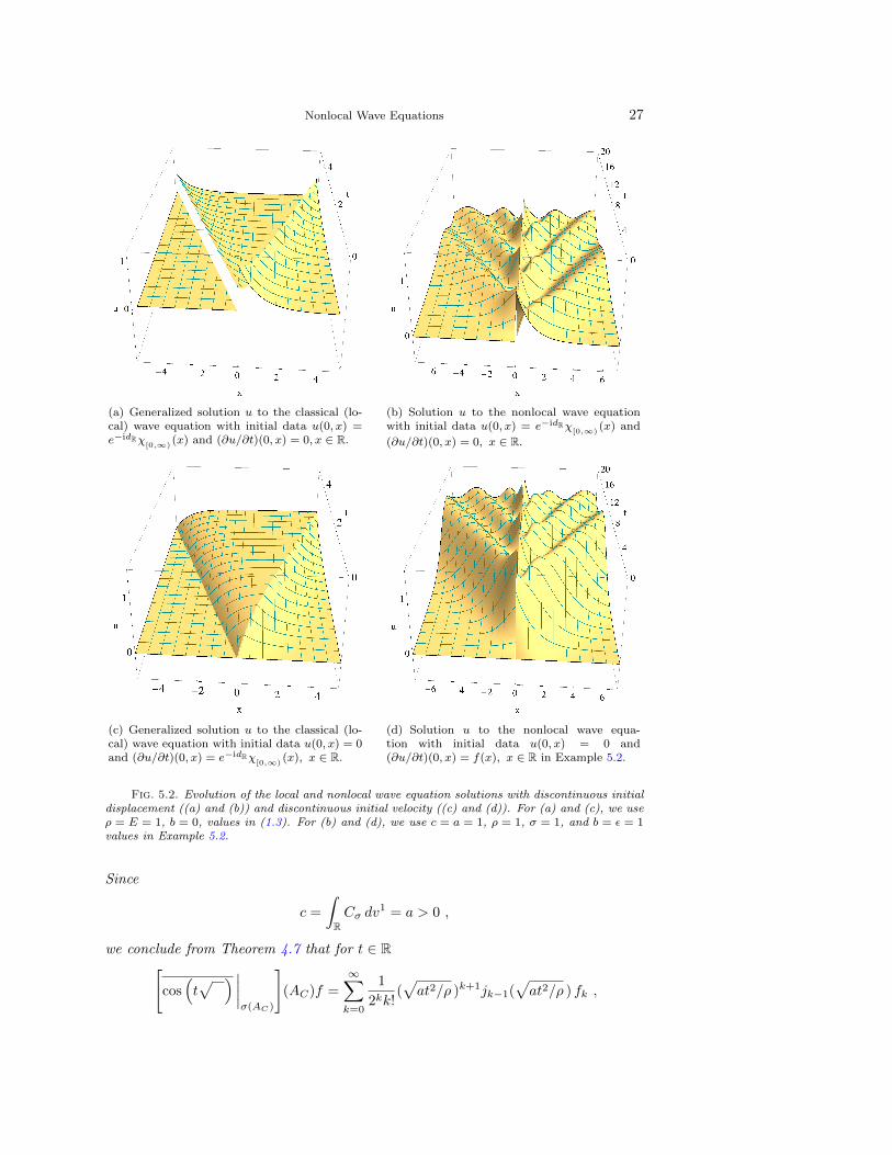
Nonlocal Wave Equations 27
(a) Generalized solution u to the classical (lo-cal) wave equation with initial data u(0, x) =e−idRχ
[0,∞)(x) and (∂u/∂t)(0, x) = 0, x ∈ R.
(b) Solution u to the nonlocal wave equationwith initial data u(0, x) = e−idRχ
[0,∞)(x) and
(∂u/∂t)(0, x) = 0, x ∈ R.
(c) Generalized solution u to the classical (lo-cal) wave equation with initial data u(0, x) = 0and (∂u/∂t)(0, x) = e−idRχ
[0,∞)(x), x ∈ R.
(d) Solution u to the nonlocal wave equa-tion with initial data u(0, x) = 0 and(∂u/∂t)(0, x) = f(x), x ∈ R in Example 5.2.
Fig. 5.2. Evolution of the local and nonlocal wave equation solutions with discontinuous initialdisplacement ((a) and (b)) and discontinuous initial velocity ((c) and (d)). For (a) and (c), we useρ = E = 1, b = 0, values in (1.3). For (b) and (d), we use c = a = 1, ρ = 1, σ = 1, and b = ε = 1values in Example 5.2.
Since
c =
∫RCσ dv
1 = a > 0 ,
we conclude from Theorem 4.7 that for t ∈ R[cos(t√ )∣∣∣∣
σ(AC)
](AC)f =
∞∑k=0
1
2kk!(√at2/ρ )k+1jk−1(
√at2/ρ ) fk ,

28 Horst R. Beyer and Burak Aksoylu and Fatih Celiker[sin(t√ )√
∣∣∣∣σ(AC)
](AC)f = t
∞∑k=0
1
2kk!(√at2/ρ )kjk(
√at2/ρ ) fk , (5.2)
where
f0 := b e−ε.idR · χ[0,∞)
,
fk(x) :=2b
πe(
εσ2
√2k)
2
e−εx erfc
(εσ
2
√2k − x
σ√
2k
)=
b√
2π√kσ2
e−εx∫ x
−∞e−u
2/(2kσ2) · eεu du
for every x ∈ R and k ∈ N∗, and where AC is as in Lemma 3.2.In the classical wave equation, as expected, discontinuities propagate along the
characteristics; see Figures 5.2(a) and 5.2(c) for vanishing initial velocity and dis-placement, respectively. On the other hand, in the nonlocal case, the discontinuityremains in the same place for all time; see Figures 5.2(b) and 5.2(d) for vanishinginitial velocity and displacement, respectively. This confirms the results given in [69].
6. Conclusion. Our result that the governing operator is a bounded func-tion of the classical local operator for scalar-valued functions should be generalizableto vector-valued case. Our notable result that the governing operator AC of theperidynamic wave equation is a bounded function of the classical governing operatorhas far reaching consequences. It enables the comparison of peridynamic solutionsto those of classical elasticity. The remarkable implication is that it opens the possi-bly of defining peridynamic-type operators on bounded domains as functions of thecorresponding classical operator. Since the classical operator is defined through localboundary conditions, the functions inherit this knowledge. This observation opens agateway to incorporate local boundary conditions into nonlocal theories, which hasvital implications for numerical treatment of nonlocal problems. This is the subjectof our companion paper [2].
We expect that the expansions in Theorems 4.3 and 4.5 can be used for obtainingthe large time asymptotic of solutions of the nonlocal wave equation. In the classicalcase, as expected, we observe the propagation of waves along characteristics. In thenonlocal case, we observe oscillatory recurrent wave separation. We think that thisphenomenon is worth investigating. On the other hand, we observe that discontinuityremains stationary in the nonlocal case, whereas, it is well-known that discontinuitiespropagate along characteristics. We hold that this fundamentally difference is oneof the most distinguishing feature of PD. In conclusion, we believe that we addedvaluable tools to the of arsenal of methods to analyze nonlocal problems.
Appendix A. Some Proofs from Section 2.
A.1. Instability of Solutions. We give a proof of Theorem 2.3.Proof. Since σ(A) is bounded from below, we can define
λ0 := inf{λ ∈ σ(A)} .
Furthermore, since σ(A) is closed, λ0 ∈ σ(A) and since
σ(A) ∩ (−∞, 0) 6= ∅ ,
we conclude that λ0 < 0. Furthermore, let f ∈ C(R,R) such that f |[0,∞) is boundedand such that f |(−∞,0] is positive and decreasing. In particular, this implies that

Nonlocal Wave Equations 29
f |σ(A) ∈ Us(σ(A)) and also that f2|(−∞,0] is positive and decreasing. Furthermore,let 0 < ε < |λ0|. Then there is ξ ∈ D(A) such that
η := (χ[λ0,λ0+ε]
|σ(A))(A)ξ 6= 0X .
Otherwise, since D(A) is in particular dense in X,
(χ[λ0,λ0+ε]
|σ(A))(A) = 0L(X,X) ,
in contradiction to the fact that λ0 ∈ σ(A). In particular, since
(χ[λ0,λ0+ε]
|σ(A))(A)
and A commute, it follows that η ∈ D(A).Furthermore,
‖(f |σ(A))(A)η‖2 = 〈(f |σ(A))(A)η|(f |σ(A))(A)η〉 = 〈η|(f |σ(A))2(A)η〉
= 〈ξ|(χ[λ0,λ0+ε]
|σ(A))(A)(f |σ(A))2(A)ξ〉 =
∫σ(A)
χ[λ0,λ0+ε]
· f2 dψξ
>∫σ(A)
χ[λ0,λ0+ε]
· [f(λ0 + ε)]2 dψξ = [f(λ0 + ε)]2∫σ(A)
χ[λ0,λ0+ε]
dψξ
= [f(λ0 + ε)]2 · ‖η‖2.
In particular, we conclude that∥∥∥∥∥[
cos(t√ )∣∣∣∣
σ(A)
](A)η
∥∥∥∥∥ > cosh(t√|λ0 + ε| ) · ‖η‖
for all t ∈ R. Since ε is otherwise arbitrary, the latter implies that∥∥∥∥∥[
cos(t√ )∣∣∣∣
σ(A)
](A)η
∥∥∥∥∥ > cosh(t√|λ0| ) · ‖η‖ >
1
2et√|λ0| · ‖η‖.
A.2. Solutions of Inhomogeneous Wave Equations. We give a proofof Theorem 2.5.
Proof. In a first step, we note for λ > 0 that
sin((t− τ)
√ )√ (λ) =
sin[(t− τ)√λ ]√
λ
=sin(t√λ )√
λcos(τ
√λ )− cos(t
√λ )
sin(τ√λ )√
λ
=sin(t√ )√ (λ) · cos
(τ√ )
(λ)− cos(t√ )
(λ) ·sin(τ√ )√ (λ) .
Since
sin((t− τ)
√ )√ ,
sin(t√ )√ , cos
(τ√ )
, cos(t√ )
,sin(τ√ )√ ,

30 Horst R. Beyer and Burak Aksoylu and Fatih Celiker
are entire functions, this implies that
sin((t− τ)
√ )√ (λ)
=sin(t√ )√ (λ) · cos
(τ√ )
(λ)− cos(t√ )
(λ) ·sin(τ√ )√ (λ) ,
for every λ ∈ C and hence, by application of the spectral theorem for densely-defined,self-adjoint linear operators in Hilbert spaces, that[
sin((t− τ)
√ )√
∣∣∣∣σ(A)
](A)f(τ)
=
{[sin(t√ )√
∣∣∣∣σ(A)
](A)
[cos(τ√ )∣∣∣∣
σ(A)
](A)
−
[cos(t√ )
(λ)
∣∣∣∣σ(A)
](A)
[sin(τ√ )√
∣∣∣∣σ(A)
](A)
}f(τ)
= b(t)a(τ)f(τ)− a(t)b(τ)f(τ)
for all t, τ ∈ R, where a, b : R→ L(X,X) are defined by
a(t) :=
[cos(t√ )
(λ)
∣∣∣∣σ(A)
](A) , b(t) :=
[sin(t√ )√
∣∣∣∣σ(A)
](A) ,
for every t ∈ R. In the following, for ξ ∈ D(A), we are going to use that the maps
(R→ X, t 7→ a(t)ξ ) and (R→ X, t 7→ b(t)ξ )
are differentiable with derivatives
(R→ X, t 7→ −b(t)Aξ ) and (R→ X, t 7→ a(t)ξ ) ,
respectively. We note that, as a consequence of the spectral theorem for densely-defined, self-adjoint linear operators in Hilbert spaces, that a, b are strongly continu-ous and that
a(t)D(A) ⊂ D(A) , b(t)D(A) ⊂ D(A) ,
for every t ∈ R. Also for every k ∈ UsC(σ(A)), k(A)D(A) ⊂ D(A) and for ξ ∈ D(A)
‖k(A)ξ‖2A = ‖k(A)ξ‖2 +‖Ak(A)ξ‖2 = ‖k(A)ξ‖2 +‖k(A)Aξ‖2[6 ‖k(A)‖2Op · ‖ξ‖2A
].
Hence a, b induce strongly continuous maps from R to XA, which we indicate with thesame symbols, and where XA := (D(A), ‖ ‖A). In addition, we note that the inclusionι of XA into X is continuous. In the next step, we observe for a strongly continuousc : R→ L(XA, XA) and a continuous g : R→ XA that
‖c(t+ h)g(t+ h)− c(t)g(t)‖A= ‖c(t+ h)g(t+ h)− c(t+ h)g(t) + c(t+ h)g(t)− c(t)g(t)‖A= ‖c(t+ h)[g(t+ h)− g(t)]A + [c(t+ h)− c(t)]g(t)‖A

Nonlocal Wave Equations 31
6 ‖c(t+ h)‖ · ‖g(t+ h)− g(t)‖A + ‖c(t+ h)g(t)− c(t)g(t)‖A
and hence that (R→ XA, t 7→ c(t)g(t)) is continuous as well as that(R→ XA, t 7→
∫ A
It
c(τ)g(τ)dτ
),
where∫ A
denotes weak integration in XA, is differentiable with derivative
(R→ XA, t 7→ c(t)g(t)) .
We conclude for every t ∈ R that
b(t)
∫ A
It
a(τ)f(τ) dτ − a(t)
∫ A
It
b(τ)f(τ) dτ
=
∫ A
It
[b(t)a(τ)f(τ)− a(t)b(τ)f(τ)] dτ
=
∫ A
It
[sin((t− τ)
√ )√
∣∣∣∣σ(A)
](A)f(τ) dτ = v(t) .
Furthermore, we observe for c : R → L(X,X), g : R → Xsuch that Ran(g) ⊂ D(A),t ∈ R and h ∈ R∗ that
1
h[c(t+ h)g(t+ h)− c(t)g(t)]
=1
h[c(t+ h)g(t+ h)− c(t+ h)g(t) + c(t+ h)g(t)− c(t)g(t)]
= c(t+ h)1
h[g(t+ h)− g(t)] +
1
h[c(t+ h)− c(t)]g(t)
= c(t)1
h[g(t+ h)− g(t)] +
1
h[c(t+ h)g(t)− c(t)g(t)]
+ [c(t+ h)− c(t)] 1
h[g(t+ h)− g(t)]
and hence that
1
h[a(t+ h)g(t+ h)− a(t)g(t)]− a(t)g ′(t) + b(t)Ag(t)
= a(t)
{1
h[g(t+ h)− g(t)]− g ′(t)
}+
1
h[a(t+ h)g(t)− a(t)g(t)] + b(t)Ag(t)
+ [a(t+ h)− a(t)]
{1
h[g(t+ h)− g(t)]− g ′(t)
}+ [a(t+ h)− a(t)]g ′(t) ,
1
h[b(t+ h)g(t+ h)− b(t)g(t)]− b(t)g ′(t)− a(t)g(t)
= b(t)
{1
h[g(t+ h)− g(t)]− g ′(t)
}+
1
h[b(t+ h)g(t)− b(t)g(t)]− a(t)g(t)
+ [b(t+ h)− b(t)]{
1
h[g(t+ h)− g(t)]− g ′(t)
}+ [b(t+ h)− b(t)]g ′(t) .

32 Horst R. Beyer and Burak Aksoylu and Fatih Celiker
This implies that
(R→ X, t 7→ a(t)g(t)) , (R→ X, t 7→ b(t)g(t))
are differentiable with derivatives
(R→ X, t 7→ a(t)g ′(t)− b(t)Ag(t)) , (R→ X, t 7→ b(t)g ′(t) + a(t)g(t)) ,
respectively. Application of the latter to v gives for t ∈ R
v ′(t) = b(t)a(t)f(t) + a(t)
∫ A
It
a(τ)f(τ) dτ − a(t)b(t)f(t) + b(t)A
∫ A
It
b(τ)f(τ) dτ
= a(t)
∫ A
It
a(τ)f(τ) dτ + b(t)
∫It
b(τ)Af(τ) dτ
= a(t)
∫ A
It
a(τ)f(τ) dτ + b(t)
∫ A
It
b(τ)Af(τ) dτ ,
where∫
denotes weak integration in X, and that
v ′′(t)
= a(t)a(t)f(t)− b(t)A∫ A
It
a(τ)f(τ) dτ + b(t)b(t)Af(t) + a(t)
∫It
b(τ)Af(τ) dτ
= a(t)a(t)f(t) + b(t)b(t)Af(t)− b(t)A∫ A
It
a(τ)f(τ) dτ + a(t)A
∫ A
It
b(τ)f(τ) dτ
= f(t)−Av(t) .
A.3. Conservation Laws Induced by Symmetries. We give a proof ofTheorem 2.4.
Proof. Part (i): Let t ∈ I and h ∈ R such that t+ h ∈ I. Then
ju,v(t+ h)− ju,v(t)h
= h−1 [〈u(t+ h)|v′(t+ h)〉 − 〈u′(t+ h)|v(t+ h)〉 − 〈u(t)|v′(t)〉+ 〈u′(t)|v(t)〉]= h−1 [〈u(t+ h)− u(t)|v′(t+ h)〉+ 〈u(t)|v′(t+ h)− v′(t)〉
− 〈u′(t+ h)|v(t+ h)− v(t)〉 − 〈u′(t+ h)− u′(t)|v(t)〉] .
Hence it follows that ju,v is differentiable in t with derivative
j′u,v(t) = 〈u(t)|(v′)′(t)〉 − 〈(u′)′(t)|v(t)〉 = 〈u(t)|(v′)′(t)〉 − 〈(u′)′(t)|v(t)〉= −〈u(t)|Av(t)〉+ 〈Au(t)|v(t)〉 = 0 .
From the latter, we conclude that the derivative of ju,v vanishes and hence that ju,vis a constant function.Part (ii): Since A ◦ B ⊃ B ◦ A, it follows that B(D(A)) ⊂ D(A). Hence B ◦ u is atwice continuously differentiable map assuming values in D(A) and satisfying
(B ◦ u) ′′(t) = Bu ′′(t) = −BAu(t) = −AB u(t) = −A(B ◦ u)(t)

Nonlocal Wave Equations 33
for all t ∈ R. According to Part (i) this implies that ju,B◦u : R→ C, defined by
ju,B◦u(t) := 〈u(t)|Bu′(t)〉 − 〈u′(t)|Bu(t)〉
for every t ∈ R, is constant.Part (iii): For the proof, let UB : R → L(X,X) be the strongly continuous one-parameter group that is generated by B. This implies that
D(B) = {ξ ∈ X : limt→0,t6=0
1
t(UB(t)− idX)ξ exists} ,
Bξ =1
ilim
t→0,t6=0
1
t(UB(t)− idX)ξ
for every ξ ∈ D(B). Since A and B commute, every f(B), where f ∈ UsC(σ(B)) andσ(B) denotes the spectrum of B, commutes with A, i.e., satisfies
A ◦ f(B) ⊃ f(B) ◦A .
Hence it follows from Part (ii) that
ju,fs(B)(t) := 〈u(t)|fs(B)u′(t)〉 − 〈u′(t)|fs(B)u(t)〉
for every t ∈ R, is constant, where
fs(λ) :=1
is
(eisλ − 1
)for every λ ∈ σ(B) and s > 0. Also, since A and B commute, every g(A), whereg ∈ UsC(σ(A)) and σ(A) denotes the spectrum of A, commutes with B, i.e., satisfies
B ◦ g(A) ⊃ g(A) ◦B ,
which implies that
g(A)(D(B)) ⊂ D(B)
and hence also that
g(A)(D(A) ∩D(B)) ⊂ D(A) ∩D(B) .
Therefore, we conclude from Theorem 2.1, since u(0), u′(0) ∈ D(A) ∩ D(B), thatRan(u),Ran(u′) ⊂ D(A) ∩D(B). As a consequence, for every t ∈ R,
lims→0
ju,fs(B)(t) = 〈u(t)|Bu′(t)〉 − 〈u′(t)|Bu(t)〉 .
Finally, since ju,fs(B) is a constant function for s > 0, we conclude that
ju,B(t) := 〈u(t)|Bu′(t)〉 − 〈u′(t)|Bu(t)〉
for every t ∈ R, is a constant function.

34 Horst R. Beyer and Burak Aksoylu and Fatih Celiker
REFERENCES
[1] H. G. Aksoy and E. Senocak, Discontinuous Galerkin method based on peridynamic theoryfor linear elasticity, Int. J. Numer. Methods Engrg, 88 (2011), pp. 673–692.
[2] B. Aksoylu, H. R. Beyer, and F. Celiker, Incorporating local boundary conditions intononlocal theories. In preparation, 2014.
[3] B. Aksoylu and T. Mengesha, Results on nonlocal boundary value problems, NumericalFunctional Analysis and Optimization, 31 (2010), pp. 1301–1317.
[4] B. Aksoylu and M. L. Parks, Variational theory and domain decomposition for nonlocalproblems, Applied Mathematics and Computation, 217 (2011), pp. 6498–6515.
[5] B. Aksoylu and Z. Unlu, Conditioning analysis of nonlocal integral operators in fractionalSobolev spaces, SIAM J. Numer. Anal., 52 (2014), pp. 653–677.
[6] B. Alali and R. Lipton, Multiscale dynamics of heterogeneous media in the peridynamicformulation, J. Elasticity, 106 (2012), pp. 71–103.
[7] G. Alberti and G. Bellettini, A nonlocal anisotropic model for phase transition. asymptoticbehaviour of rescaled, European J. Appl. Math., 9 (1998), pp. 261–284.
[8] , A nonlocal anisotropic model for phase transition. Part I: the optimal profile problem,Math. Ann., 310 (1998), pp. 527–560.
[9] F. Andreu-Vaillo, J. M. Mazon, J. D. Rossi, and J. Toledo-Melero, Nonlocal DiffusionProblems, vol. 165 of Mathematical Surveys and Monographs, American MathematicalSociety and Real Socied Matematica Espanola, 2010.
[10] E. Askari, F. Bobaru, R. B. Lehoucq, M. L. Parks, S. A. Silling, and O. Weckner,Peridynamics for multiscale materials modeling, Journal of Physics: Conference Series,125 (2008), p. (012078). SciDAC 2008, Seattle, Washington, July 13-17, 2008.
[11] H. R. Beyer, Beyond partial differential equations: A course on linear and quasi-linear ab-stract hyperbolic evolution equations, vol. 1898 of Lecture Notes in Mathematics, Springer:Berlin, 2007.
[12] M. Bodnar and J. J. L. Velazquez, An integro-differential equation arising as a limit ofindividual cell-based models, J. Differential Equations, 222 (2006), pp. 341–380.
[13] C. Carrillo and P. Fife, Spatial effects in discrete generation population models, J. Math.Biol., 50 (2005), pp. 161–188.
[14] E. Celik, I. Guven, and E. Madenci, Simulations of nanowire bend tests for extractingmechanical properties, Theoretical and Applied Fracture Mechanics, 55 (2011), pp. 185–191.
[15] X. Chen and M. Gunzburger, Continuous and discontinuous finite element methods fora peridynamics model of mechanics, Comput. Methods Appl. Mech. Engrg, 200 (2011),pp. 1237–1250.
[16] Q. Du, M. Gunzburger, R. B. Lehoucq, and K. Zhou, Analysis and approximation ofnonlocal diffusion problems with volume constraints, SIAM Rev., 54 (2012), pp. 667–696.
[17] , Analysis of the volume-constrained peridynamic Navier equation of linear elasticity, J.Elasticity, 113 (2013), pp. 193–217.
[18] , A nonlocal vector calculus, nonlocal volume-constrained problems, and nonlocal balancelaws, Math. Mod. Meth. Appl. Sci., 23 (2013), pp. 493–540.
[19] Q. Du, L. Ju, L. Tian, and K. Zhou, A posteriori error analysis of finite element method forlinear nonlocal diffusion and peridynamic models, Math. Comp., (2013), pp. 1889–1922.
[20] Q. Du, J. R. Kamm, R. B. Lehoucq, and M. L. Parks, A new approach for a nonlocal,nonlinear conservation law, SIAM Journal on Applied Mathematics, 72 (2012), pp. 464–487.
[21] Q. Du and R. Lipton, Peridynamics, Fracture, and Nonlocal Continuum Models. SIAM News,Volume 47, Number 3, April 2014.
[22] Q. Du, L. Tian, and X. Zhao, A convergent adaptive finite element algorithm for nonlocaldiffusion and peridynamic models. to appear in SIAM J. Numer. Anal., 2013.
[23] Q. Du and K. Zhou, Mathematical analysis for the peridynamic nonlocal continuum theory,ESAIM: Mathematical Modelling and Numerical Analysis, 45 (2011), pp. 217–234.
[24] N. Duruk, H. A. Erbay, and A. Erkip, A higher-order Boussinesq equation in locally non-linear theory of one-dimensional non-local elasticity, IMA Journal of Applied Mathematics,74 (2009), pp. 97–106.
[25] , Global existence and blow-up for a class of nonlocal nonlinear Cauchy problems arisingin elasticity, Nonlinearity, 23 (2010), pp. 107–118.
[26] , Blow-up and global existence for a general class of nonlocal nonlinear coupled waveequations, J. Differential Equations, (2011), pp. 1448–1459.
[27] E. Emmrich, R. B. Lehoucq, and D. Puhst, Peridynamics: a nonlocal continuum theory, in

Nonlocal Wave Equations 35
Meshfree Methods for Partial Differential Equations VI, M. Griebel and M. A. Schweitzer,eds., vol. 89, Springer, 2013, pp. 45–65.
[28] E. Emmrich and O. Weckner, On the well-posedness of the linear peridynamic model andits convergence towards the Navier equation of linear elasticity, Commun. Math. Sci., 5(2007), pp. 851–864.
[29] , The peridynamic equation and its spatial discretization, Math. Model. Anal., 12 (2007),pp. 17–27.
[30] N. Fournier and P. Laurnecot, Well-posedness of smoluchowski’s coagulation equation fora class of homogeneous kernels, J. Funct. Anal., 233 (2006), pp. 351–379.
[31] G. Gilboa and S. Osher, Nonlocal operators with applications to image processing, MultiscaleModeling and Simulation, 7 (2008), pp. 1005–1028.
[32] M. D. Gunzburger and R. B. Lehoucq, A nonlocal vector calculus with application to non-local boundary value problems, Multiscale Model. Simul., 8 (2010), pp. 1581–1598.
[33] B. Hinds and P. Radu, Dirichlet’s principle and wellposedness of steady state solutionsfor a nonlocal peridynamics model, Applied Mathematics and Computation, 219 (2012),pp. 1411–1419.
[34] V. Hutson, J. S. Pym, and M. J. Cloud, Applications of Functional Analysis and OperatorTheory, Elsevier, 2 ed., 2005.
[35] K. Joergens, Spectral theory of second-order ordinary differential operators, 1962. Lecturesdelivered at the University of Aarhus 1962/63.
[36] J. F. Kalthoff and S. Winkler, Failure mode transition at high rates of shear loading, inImpact Loading and Dynamic Behavior of Materials, C. Chiem, H.-D.Kunze, and L. Meyer,eds., vol. 1, DGM Informationsgesellschaft Verlag, 1988, pp. 185–195.
[37] B. Kilic, A. Agwai, and E. Madenci, Peridynamic theory for progressive damage predictionin centre-cracked composite laminates, Composite Structures, 90 (2009), pp. 141–151.
[38] B. Kilic and E. Madenci, Prediction of crack paths in a quenched glass plate by using peri-dynamic theory, Int. J. Fract., 156 (2009), pp. 165–177.
[39] , Coupling of peridynamic theory and finite element method, Journal of Mechanics ofMaterials and Structures, 5 (2010), pp. 707–733.
[40] S. Kindermann, S. Osher, and P. W. Jones, Deblurring and denoising of images by nonlocalfunctionals, Multiscale Model. Simul., 4 (2005), pp. 1091–1115.
[41] R. Lehoucq and S. Silling, Convergence of peridynamics to classical elasticity, J. Elasticity,93 (2008), pp. 13–37. doi:10.1007/s10659-008-9163-3.
[42] , Force flux and the peridynamic stress tensor, J. Mech. Phys. Solids, 56 (2008), pp. 1566–1577.
[43] R. B. Lehoucq and S. Silling, Peridynamic theory of solid mechanics, Advances in AppliedMechanics, 44 (2010), pp. 73–168.
[44] R. Lipton, Dynamic brittle fracture as a small horizon limit of peridynamics, J. Elasticity,(2014). DOI: 10.1007/s10659-013-9463-0.
[45] E. Madenci and E. Oterkus, Peridynamic Theory and Its Applications, Springer, 2014.[46] T. Mengesha, Nonlocal Korn-type characterization of Sobolev vector fields, Communication
in Comtemporary Mathematics, 14 (2012), pp. 1250028, (28 pp.).[47] T. Mengesha and Q. Du, Analysis of a scalar peridynamic model for sign changing kernel,
Disc. Cont. Dyn. Sys. B, 18 (2013), pp. 1415–1437.[48] Y. Mikata, Analytical solutions of peristatic and peridynamics problems for a 1D infinite rod,
International Journal of Solids and Structures, 49 (2012), pp. 2887–2897.[49] S. G. Mikhlin, Mathematical physics, an advanced course, North-Holland: Amsterdam, 1970.[50] A. Mogilner and Leah Edelstein-Keshet, A non-local model for a swarm, J. Math. Biol.,
38 (1999), pp. 534–570.[51] F. W. J. Olver, D. W. Lozier, R. F. Boisvert, and C. W. Clark, eds., NIST Handbook of
Mathematical Functions, Cambridge University Press : New York, 2010.[52] E. Oterkus and E. Madenci, Peridynamic analysis of fiber reinforced composite materials,
Journal of Mechanics of Materials and Structures, 7 (2012), pp. 45–84.[53] , Peridynamic theory for damage initiation and growth in composite laminate, Key En-
gineering Materials, 488–489 (2012), pp. 355–358.[54] E. Oterkus, E. Madenci, O. Weckner, S. S. Silling, P. Bogert, and A. Tessler, Com-
bined finite element and peridynamic analyses for predicting failure in a stiffened compositecurved panel with a central slot, Composite Structures, 94 (2012), pp. 839–850.
[55] A. Pazy, Semigroups of Linear Operators and Applications to Partial Differential Equations,New York: Springer, 1983.
[56] M. Reed and B. Simon, Methods of modern mathematical physics, vol. I, II, III, IV, Academic:New York, 1980, 1975, 1979, 1978.

36 Horst R. Beyer and Burak Aksoylu and Fatih Celiker
[57] W. Rudin, Functional Analysis, New York: McGraw-Hill, 1991.[58] P. Seleson, S. Beneddine, and S. Prudhomme, A force-based coupling scheme for peridy-
namics and classical elasticity, Computational Materials Science, 66 (2013), pp. 34–49.[59] P. Seleson, M. Gunzburger, and M. L. Parks, Interface problems in nonlocal diffusion
and sharp transitions between local and nonlocal domains, Computer Methods in AppliedMechanics and Engineering, 266 (2013), pp. 185–204.
[60] , Peridynamic state-based models and the embedded-atom model, Communications inComputational Physics, 15 (2014), pp. 179–205.
[61] P. Seleson and M. L. Parks, On the role of the influence function in the peridynamic theory,International Journal for Multiscale Computational Engineering, 9 (2011), pp. 689–706.
[62] P. Seleson, M. L. Parks, M. Gunzburger, and R. B. Lehoucq, Peridynamics as an up-scaling of molecular dynamics, Multiscale Model. Simul., 8 (2009), pp. 204–227.
[63] S. Silling, Reformulation of elasticity theory for discontinuities and long-range forces, J. Mech.Phys. Solids, 48 (2000), pp. 175–209.
[64] S. A. Silling, Dynamic fracture modeling with a meshfree peridynamic code, in ComputationalFluid and Solid Mechanics, K. Bathe, ed., Elsevier, 2003, pp. 641–644.
[65] S. A. Silling and F. Bobaru, Peridynamic 3D problems of nanofiber networks and carbonnanotube-reinforced composites, in Materials and Design: Proc. Numiform, American In-stitute of Physics, 2004, pp. 1565–1570.
[66] , Peridynamic modeling of membranes and fibers, Int. J. Nonlinear Mech., 40 (2005),pp. 395–409.
[67] S. A. Silling, M. Zimmermann, and R. Abeyaratne, Deformation of a peridynamic bar, J.Elasticity, 73 (2003), pp. 173–190.
[68] X. Tian and Q. Du, Analysis and comparison of different approximations to nonlocal diffusionand linear peridynamic equations, SIAM J. Numer. Anal., (2013). To appear.
[69] O. Weckner and R. Abeyaratne, The effect of long-range forces on the dynamics of a bar,Journal of the Mechanics and Physics of Solids, 53 (2005), pp. 705–728.
[70] J. Weidmann, Linear Operators in Hilbert Spaces, vol. 68 of Graduate Texts in Mathematics,Springer-Verlag, 1980.
[71] K. Yosida, Functional Analysis, Berlin: Springer, 1980.[72] K. Zhou and Q. Du, Mathematical and numerical analysis of linear peridynamic models with
nonlocal boundary conditions, SIAM J. Numer. Anal., 48 (2010), pp. 1759–1780.