finite elements for helmholtz equations with a nonlocal

FINITE ELEMENTS FOR HELMHOLTZ EQUATIONS WITH A1

NONLOCAL BOUNDARY CONDITION∗2

ROBERT C. KIRBY† , ANDREAS KLOCKNER‡ , AND BEN SEPANSKI§3

Abstract. Numerical resolution of exterior Helmholtz problems requires some approach to do-4main truncation. As an alternative to approximate nonreflecting boundary conditions and invocation5of the Dirichlet-to-Neumann map, we introduce a new, nonlocal boundary condition. This condition6is exact and requires the evaluation of layer potentials involving the free space Green’s function. How-7ever, it seems to work in general unstructured geometry, and Galerkin finite element discretization8leads to convergence under the usual mesh constraints imposed by Garding-type inequalities. The9nonlocal boundary conditions are readily approximated by fast multipole methods, and the resulting10linear system can be preconditioned by the purely local operator involving transmission boundary11conditions.12

Key words. finite element method, Helmholtz, boundary conditions, layer potentials13

AMS subject classifications. 65N30, 65N80, 65F0814

1. Introduction. The exterior Helmholtz problem plays an essential role in scat-15

tering problems and also serves as a starting point to consider exterior problems in16

electromagnetics and problems in other unbounded domains such as waveguides. The17

literature contains several techniques to address the challenge that unbounded do-18

mains pose for numerical methods. Essentially, these techniques include some combi-19

nation of truncating the domain to a bounded one, posing boundary conditions that20

enforce (or approximate) the Sommerfeld condition on the newly-introduced bound-21

ary, and/or modifying the PDE near the computational boundary to absorb any22

reflected waves.23

An early paper on finite elements for the exterior problem is [?], where the do-24

main is truncated at radius R and an approximate radiation condition is posed at R.25

Although the error estimates contain a factor of R−2, it is also possible to carefully26

increase the mesh spacing near the boundary, somewhat mitigating the cost of a large27

domain. Perfectly matched layers [?] modify the PDE near the boundary of the com-28

putational domain, changing the coefficient of the elliptic term to ‘absorb’ outgoing29

waves. While such methods allow small effective computational domains, the result-30

ing linear systems do not yield readily to standard iterative techniques like multigrid,31

although we refer to recent work [?] that poses a domain decomposition strategy to32

use a direct solver only near the boundary and standard iterative techniques inside.33

There is also considerable literature on nonlocal boundary conditions for domain34

truncation. Following early work [?, ?, ?], one can use a Dirichlet-to-Neumann (DtN)35

operator on the artificial boundary to enforce proper far-field behavior. Givoli [?]36

provides a survey of similar techniques and local conditions as well, and [?, ?] give37

techniques for the time rather than frequency domain case. The DtN is typically given38

∗Submitted to the editors DATE.Funding: This work was funded by NSF awards SHF-1909176 and SHF-1911019. This material

is based upon work supported by the U.S. Department of Energy, Office of Science, Office of AdvancedScientific Computing Research, Department of Energy Computational Science Graduate Fellowshipunder Award Number DE-SC0021110.†Baylor University, Department of Mathematics, Waco, TX (robert [email protected], https://

sites.baylor.edu/robert kirby/).‡Department Computer Science, University of Illinois at Urbana-Champaign, Urbana, IL (an-

[email protected])§University of Texas, Department of Computer Science, Austin, TX (ben [email protected])

1

This manuscript is for review purposes only.

mailto:robert\protect [email protected]

https://sites.baylor.edu/robert_kirby/

https://sites.baylor.edu/robert_kirby/

mailto:[email protected]

mailto:[email protected]

mailto:ben\protect [email protected]

2 R. C. KIRBY, A. KLOCKNER, AND B. SEPANSKI

as an infinite series (truncated in computation) obtained by separating variables. This39

limits the shape of the domain boundary, although perturbations of such domains40

and use of high-order methods are possible [?, ?, ?]. Careful error analysis for finite41

element discretizations can include the effect of truncating the infinite series as well as42

polynomial approximation error [?]. Lastly, it is worth noting that boundary integral43

equation methods solve exterior Helmholtz problems with optimal complexity (linear44

in the number of boundary degrees of freedom), however they are somewhat more45

difficult to adapt than (volume) PDE discretizing-methods to specific (and potentially46

nonlinear) near-surface physics.47

In this paper, we propose an alternative nonlocal boundary condition based on48

Green’s Theorem [?] that has several important features. Like the DtN approach,49

we have an (in principle) exact boundary condition, incurring no error in our domain50

truncation. However, because we rely on the free-space Green’s function, there is51

(again, in principle) no restriction on the shape of our computational domain. The52

layer potentials appearing in our nonlocal boundary condition can be efficiently com-53

puted by appropriate fast algorithms such as variants of the Fast Multipole Method [?].54

So, although Galerkin’s method would give matrices with dense sub-blocks, we can55

quickly compute the matrix-vector product required in a Krylov method. Because56

our nonlocal operator involves double integrals over distinct boundaries, we avoid the57

need to evaluate any singular integrals. We note that “two-boundary” approaches58

have been explored in the time-domain literature [?, ?, ?]. Finally, the local part of59

the operator (a standard finite element matrix) serves as an excellent preconditioner60

for the system, so that an optimal solver for the local part would give O(n log n)61

solution time in unstructured geometry. Our method works equally well in two and62

three space dimensions.63

Another method combining boundary integral and volumetric discretizations is64

due to Johnson and Nedelec [?, ?]. This technique encloses a compactly-supported65

volume source in a truncating boundary. Finite elements are used to compute the66

solution inside the boundary and a boundary integral method is used on the boundary67

to handle the exterior. Our present method bears some similarly, employing the same68

kind of operators. However, we require only a single finite element space and do not69

introduce additional unknowns on the domain boundary.70

In the rest of the paper, we pose the model and its finite element discretization71

in Section 2. We describe a preconditioned Krylov system for this system in Sec-72

tion 3. Our implementation, which relies on the high-level codes Firedrake [?] and73

Pytential [?], warrants some discussion, which is given in Section 4. Finally, we74

give numerical results in Section 5.75

2. Model and discretization. Let Ωc ⊂ Rd with d = 2, 3 be a bounded domain76

with boundary Γ, and Ω = Rd\Ωc its exterior. We consider the classic Helmholtz77

exterior problem on Ω78

(2.1) −∆u− κ2u = 0,79

where κ2 is nonzero wave number. It may be complex (typically with positive real80

part), and may take different forms in various application fields such as acoustics or81

electromagnetics. We also pose Neumann boundary conditions82

(2.2) ∂u∂n = f83


FEM FOR HELMHOLTZ EQUATIONS WITH A NONLOCAL BOUNDARY CONDITION 3

on the interior boundary Γ. The Sommerfeld radiation condition84

(2.3) limr→∞

rd−1

2(∂u∂r − iκu

)= 0,85

where r is the outward radial direction, must also hold. For computational purposes,86

one typically poses the problem only on a truncated domain Ω′. Hence, we impose an87

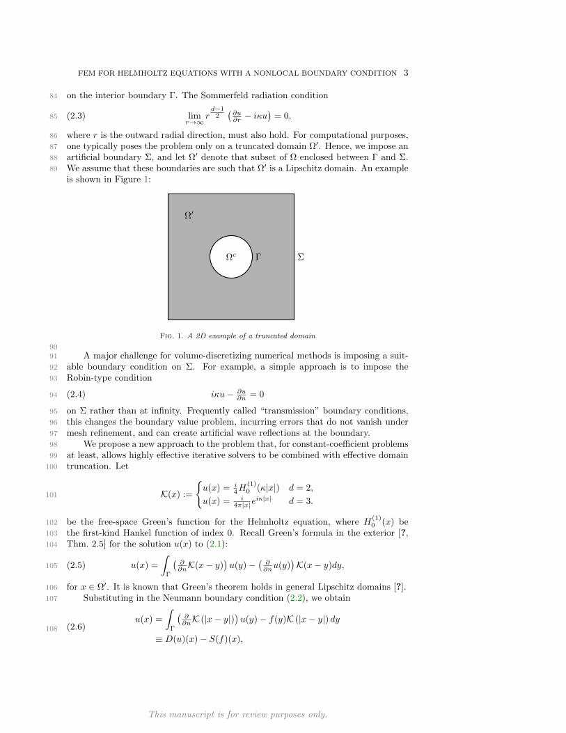
artificial boundary Σ, and let Ω′ denote that subset of Ω enclosed between Γ and Σ.88

We assume that these boundaries are such that Ω′ is a Lipschitz domain. An example89

is shown in Figure 1:

Ωc

Ω′

Γ Σ

Fig. 1. A 2D example of a truncated domain

90

A major challenge for volume-discretizing numerical methods is imposing a suit-91

able boundary condition on Σ. For example, a simple approach is to impose the92

Robin-type condition93

(2.4) iκu− ∂u∂n = 094

on Σ rather than at infinity. Frequently called “transmission” boundary conditions,95

this changes the boundary value problem, incurring errors that do not vanish under96

mesh refinement, and can create artificial wave reflections at the boundary.97

We propose a new approach to the problem that, for constant-coefficient problems98

at least, allows highly effective iterative solvers to be combined with effective domain99

truncation. Let100

K(x) :=

u(x) = i

4H(1)0 (κ|x|) d = 2,

u(x) = i4π|x|e

iκ|x| d = 3.101

be the free-space Green’s function for the Helmholtz equation, where H(1)0 (x) be102

the first-kind Hankel function of index 0. Recall Green’s formula in the exterior [?,103

Thm. 2.5] for the solution u(x) to (2.1):104

(2.5) u(x) =

∫Γ

(∂∂nK(x− y)

)u(y)−

(∂∂nu(y)

)K(x− y)dy,105

for x ∈ Ω′. It is known that Green’s theorem holds in general Lipschitz domains [?].106

Substituting in the Neumann boundary condition (2.2), we obtain107

u(x) =

∫Γ

(∂∂nK (|x− y|)

)u(y)− f(y)K (|x− y|) dy

≡ D(u)(x)− S(f)(x),

(2.6)108



for x ∈ Ω′, where109

(2.7) D(u)(x) = PV

∫Γ

(∂∂nK(x− y)

)u(y)dy110

is the double layer potential and111

(2.8) S(u)(x) =

∫Γ

K(x− y)u(y)dy112

is the single layer potential [?].113

Now, we can pose an exact nonlocal Robin-type boundary condition as follows.114

We use the representation (2.5) to write (suppressing the argument x):115

(2.9) iκu− ∂u∂n = iκ (D(u)− S(f))− ∂

∂n (D(u)− S(f)) ,116

so that over Σ,117

(2.10) ∂u∂n = iκu−

(iκ− ∂

∂n

)(D(u)− S(f)) .118

2.1. Variational Setting. We let (f, g) =∫

Ω′ f(x)g(x)dx be the standard L2119

inner product over the computational domain, and 〈f, g〉S that over some portion120

S ⊆ ∂Ω′ of its boundary. We also let Hs(Ω′) be the standard Sobolev spaces consisting121

of L2 functions with weak derivatives of order up to and including s in L2.122

When X is some Banach space, ‖ · ‖X refers to its norm. As we use several123

different norms throughout our analysis, we explicitly label each such norm to limit124

confusion.125

We give a variational formulation of the PDE and hence a standard Galerkin126

finite element discretization as follows. We take the inner product of (2.1) with any127

v ∈ H1(Ω′). Integration by parts and the Neumann boundary condition on Γ give128

(2.11) (∇u,∇v)− κ2 (u, v)− 〈 ∂u∂n , v〉Σ = 〈f, v〉Γ,129

and substituting (2.10) in for ∂u∂n on Σ gives130

(∇u,∇v)− κ2 (u, v)− iκ〈u, v〉Σ + 〈(iκ− ∂

∂n

)D(u), v〉Σ

= 〈f, v〉Γ + 〈(iκ− ∂

∂n

)S(f), v〉Σ.

(2.12)131

Hence, the solution to the Helmholtz equation (2.1) on Ω together with (2.2) and (2.3)132

satisfies the variational problem of finding u ∈ H1(Ω′) such that133

(2.13) a(u, v) = F (v)134

for all v ∈ H1(Ω′). Here, the bilinear form135

(2.14) a(u, v) = (∇u,∇v)− κ2 (u, v)− iκ〈u, v〉Σ + 〈(iκ− ∂

∂n

)D(u), v〉Σ136

consists of the standard bilinear form using transmission boundary conditions (2.4)137

augmented by nonlocal terms involving a convolution-type integral with a Green’s138

function kernel. We write a(u, v) = aL(u, v) + aNL(u, v), where139

aL(u, v) = (∇u,∇v)− κ2 (u, v)− iκ〈u, v〉Σ,aNL(u, v) = 〈

(iκ− ∂

∂n

)D(u), v〉Σ.

(2.15)140



Similarly, the linear form141

(2.16) F (v) = 〈f, v〉Γ + 〈(iκ− ∂

∂n

)S(f), v〉Σ142

involves the Neumann data on the scatterer together with its appearance in the single143

layer potential.144

By taking Vh ⊂ H1(Ω′) as any suitable finite element space, we can introduce a145

Galerkin finite element method of finding uh ∈ Vh such that146

(2.17) a(uh, vh) = F (vh)147

for all vh ∈ Vh.148

At this point, we pause compare our method to the Dirichlet-to-Neumann map149

P . (In the literature, the same operator is sometimes called the Steklov-Poincare150

operator. Generically, S-P operators convert one type of boundary data into another.)151

Replacing ∂u∂n on Σ in (2.11) with P acting on u would give152

(∇u,∇v)− κ2 (u, v) + 〈Pu, v〉Σ = 〈f, v〉Γ.153

Compared to (2.14), this appears to only have a single nonlocal term. Moreover, P is154

a symmetric elliptic operator from H1/2(Σ) into H−1/2(Σ), so that 〈Pu, u〉 ≥ 0 and155

a Garding estimate readily holds for the bilinear form. Unfortunately, the Steklov-156

Poincare operator is not typically explicitly available, and thus its application requires157

the solution of a linear system at additional computational cost, e.g. in the form of a158

boundary integral equation solve. Approximating Pu with a Fourier series is possible,159

however doing so requires separable geometry.160

2.2. Convergence theory. Our argument will rely on showing the boundedness161

of the bilinear form a and establishing a Garding-type inequality. Using standard162

techniques [?], this leads to discrete solvability and optimal a priori error estimates163

under a constraint on the maximal mesh size.164

We will rely on the trace estimates [?, ?] that since Ω′ is Lipschitz, there exists a165

constant C such that166

(2.18) ‖v‖L2(∂Ω′) ≤ C ‖v‖1/2L2(Ω′) ‖v‖

1/2H1(Ω′) ≤ C ‖v‖H1(Ω′)167

for all v ∈ H1(Ω′).168

Proposition 2.1. If the Neumann data satisfies f ∈ H− 12 (Γ), the functional F169

defined in (2.16) is a bounded linear functional on H1.170

Proof. Linearity is clear from the linearity of integration and differentiation. To171

see that it is bounded, let v ∈ H1(Ω) be given. The local portion of F is bounded172

thanks to Cauchy-Schwarz and the second trace estimate in (2.18). For the nonlocal173

portion, it is known [?] that S(f) ∈ H1(Ω′) and so it has a normal derivative on Σ in174

H−1/2(Σ).175

The following result implies both the boundedness of aNL on H1 × H1 and is176

critical to establishing the Garding inequality:177

Lemma 2.2. There exists a CNL > 0 such that for all u, v ∈ H1(Ω′),178

(2.19) |aNL(u, v)| ≤ CNL ‖u‖L2(Γ) ‖v‖L2(Σ) .179



Proof. First, we simplify the notation by writing the first argument in aNL as180

(2.20)(iκ− ∂

∂n

)D(u) =

(iκ− ∂

∂n

) ∫Γ

K(x− y)u(y)dy,181

From the properties of the kernel, K(x − y) is smooth and bounded provided that182

‖x− y‖ is bounded below away from zero. Since we have x ∈ Σ and y ∈ Γ, this is the183

case as long as the truncating boundary stays away from the scatterer. By writing184

the normal derivative in (2.20) as the limit of a difference quotient, passing under185

the integral, and appealing to the Lebesgue Dominated Convergence Theorem in the186

usual way, we can then write187

(2.21)(iκ− ∂

∂n

)D(u) =

∫Γ

(iκ− ∂

∂n

)K(x− y)dy =

∫Γ

K(x− y)dy,188

where K(x− y) is also smooth and bounded for x and y separated. We can write the189

nonlocal bilinear form now as190

(2.22) |aNL(u, v)| =∣∣∣∣∫

Γ

∫Σ

K(x, y)u(y)v(x)dx dy

∣∣∣∣ ≤ K0

∫Γ

u(y)dy

∫Σ

v(x)dx,191

and the result holds with with CNL = K0|Γ|1/2|Σ|1/2 by the Cauchy-Schwarz inequal-192

ity.193

Proposition 2.3. There exists CB > 0 such that for all u, v ∈ H1(Ω′),194

(2.23) |a(u, v)| ≤ CB ‖u‖H1(Ω′) ‖v‖H1(Ω′) .195

Proof. Let u, v ∈ H1(Ω′). Then196

|a(u, v)| ≤ ‖∇u‖L2(Ω′) ‖∇v‖L2(Ω′)

+ κ2 ‖u‖L2(Ω′) ‖v‖L2(Ω′) + κ ‖u‖L2(Σ) ‖v‖L2(Σ) + |aNL(u, v)|,(2.24)197

and the proof is finished by applying the previous Lemma and trace theorem.198

The bilinear form a satisfies a Garding inequality. That is, shifting a by a multiple199

of the L2 inner product renders a coercive bilinear form. For complex Hilbert spaces,200

it is sufficient to demonstrate that the real part itself is coercive.201

Proposition 2.4. There exists a real number M and an α > 0 such that202

(2.25) Re(a(u, u)) +M ‖u‖2L2(Ω′) ≥ α ‖u‖2H1(Ω′) .203

Proof. We calculate204

(2.26) a(u, u) = ‖∇u‖2L2(Ω′) − κ2 ‖u‖2L2(Ω′) − iκ ‖u‖

2L2(Σ) + aNL(u, u),205

and note that the real part of this is just206

Re(a(u, u)) = ‖∇u‖2L2(Ω′) − κ2 ‖u‖2L2(Ω′) + Re(aNL(u, u))

= ‖u‖2H1(Ω′) −(κ2 + 1

)‖u‖2L2(Ω′) + Re(aNL(u, u)).

(2.27)207

Using Lemma 2.2, the trace inequality (2.18), and a weighted Young’s inequality, we208

can bound this below by209

Re(a(u, u)) ≥ ‖u‖2H1(Ω′) − (κ2 + 1) ‖u‖2L2(Ω′) − CNL ‖u‖L2(Σ) ‖u‖L2(Γ)

≥ ‖u‖2H1(Ω′) − (κ2 + 1) ‖u‖2L2(Ω′) − CNL ‖u‖H1(Ω′) ‖u‖L2(Ω′)

≥ 12 ‖u‖

2H1(Ω′) −

(κ2 + 1 +

C2NL

2

)‖u‖2L2(Ω′) ,

(2.28)210



so (2.26) holds with α = 12 provided M ≥ κ2 +

3+C2NL

2 .211

Now, following standard techniques for general elliptic (but possibly not coercive)212

problems [?], suitably adapted for the complex-valued case, we have a general solvabil-213

ity and approximation result. We suppose that the standard abstract approximation214

result215

(2.29) infv∈Vh

‖u− v‖H1(Ω′) ≤ CAh |u|H2(Ω′)216

holds and that the solution to (2.1) is in H2(Ω′). We also require that the adjoint217

problem of finding w ∈ H1(Ω′) such that218

(2.30) a(v, w) = (f, v)219

for all v ∈ H1(Ω′) has a unique solution with regularity estimate220

(2.31) |u|H2(Ω′) ≤ CR ‖f‖L2(Ω′) .221

With these assumptions, the arguments leading to Theorem 5.7.6 of [?] give this result:222

Theorem 2.5. Under the above conditions, there exists h0 such that for h ≤ h0,223

the discrete variational problem (2.32) has a unique solution uh satisfying the error224

estimate225

(2.32) ‖u− uh‖H1(Ω′) ≤ C infv∈Vh

‖u− v‖H1(Ω′) .226

Moreover, with the same assumptions, there exists another C > 0 such that227

(2.33) ‖u− uh‖L2(Ω′) ≤ Ch ‖u− uh‖H1(Ω′) .228

Note that this is a quasi-optimal result, independent of the particular choice of poly-229

nomial spaces. So, it gives error estimates for higher-order approximations as well as230

for standard P 1 elements.231

Remark 2.6. In particular, following [?], one can show232

(2.34) h0 =

(α

2M

)1/2CBCACR

,233

and the constant C in (2.32) can be taken as 2CB

α and that in (2.33) as CBCACR.234

Remark 2.7. This convergence theory assumes the layer potentials and boundary235

integrals are evaluated exactly. These results can be extended to account for approx-236

imation to the layer potential along the lines of [?, Thm. 13.6/7] and quadrature in237

the bilinear forms using the standard theory of variational crimes [?].238

3. Linear algebra. We can effectively solve our variational formulation using239

preconditioned GMRES, which is a parameter-free algorithm approximating the solu-240

tion of a linear system Ax = b as the element of the Krylov subspace spanAibmi=0241

minimizing the equation residual. Building the subspace does not require the entries242

of A, just the action of A on vectors. Unlike conjugate gradients, GMRES is not243

restricted to operators that are symmetric and positive definite.244

For most problems arising in the discretization of PDE, the condition number245

of A degrades quickly under mesh refinement, and GMRES is most frequently used246



in conjunction with a (left) preconditioner. Mathematically, we multiply the linear247

system through by some matrix P−1:248

(3.1) P−1Ax = P−1b,249

and so the Krylov space then is span(P−1A

)iP−1bmi=0.250

The overall performance of GMRES typically is determined by two factors –251

the cost of building and applying the operators P−1 and A, and the total number252

of iterations. One hopes to obtain a per-application cost that scales linearly (or253

log-linearly) with respect to the number of unknowns in the linear system, and a254

total number of GMRES iterations that is bounded independently of the number of255

unknowns. We think of P−1 being an approximation to the inverse of some matrix256

P that somehow approximates A. In our case, we will find it useful to let P = AL,257

the local part of the operator. Then, applying P−1 might correspond to applying the258

inverse of P by a sparse direct method or perhaps just some sweeps of a multigrid259

algorithm.260

3.1. Structure of the discrete problem. By taking a standard finite element261

basis φiNi=1 for Vh, the stiffness matrix is262

(3.2) Aij = a(φj , φi) = aL(φj , φi) + aNL(φj , φi) = ALij +ANLij .263

The portion AL is the standard sparse matrix one obtains for discretization of the264

Helmholtz operator with transmission boundary conditions, while ANL contains the265

contributions for the nonlocal terms. To further consider the sparsity of this system,266

supposing we use standard P 1 basis functions and have aboutO(Nd) total vertices and267

hence basis functions. Then AL has nonzero entries corresponding to vertices sharing268

a common mesh element – typically about 6-7 nonzeros per row on two-dimensional269

triangulations and 20-30 for three-dimensional tetrahedral meshes when using linear270

basis functions. The total storage required for AL will be proportional to the number271

of vertices in the mesh.272

Explicit sparse storage of ANL, however, can be quite different. Since K involves273

a convolution-type integral over Γ,274

(3.3) ANLij = 〈(iκ− ∂

∂n

)K(φj), φi〉Σ275

will be nonzero whenever φj is supported on Γ and φi is supported on Σ. Suppose that276

we have O(Nd−1) basis functions supported on Σ and the same order on Γ. Then,277

ANL will be nonzero except for a dense logical subblock. However, each basis function278

associated with Σ will interact with each basis functions associated with Γ, so that279

the dense subblock will contain about O(N2d−2) nonzero entries. When d = 2, ANL280

has the same order of nonzeros as AL and so conceivably could be stored explicitly.281

On the other hand, when d = 3, ANL has O(N4) nonzero entries and so its storage282

dominates that of the local part AL. Consequently, a matrix-free application of ANL283

that bypasses the storage may be preferred, as described in Section 4.2.284

3.2. Operator application. From (3.2), the system matrix A = AL + ANL is285

the sum of two matrices corresponding to the local and nonlocal terms in the bilinear286

form. Although we could implement a matrix-free action of AL, we opt to assemble287

a standard sparse matrix and only apply ANL in a matrix-free fashion as follows.288

Recall that ANL = aNL(φj , φi) = 〈(iκ− ∂

∂n

)D(φj), φi〉. Any vector x ∈ RdimVh289

can be identified uniquely with some vh in the finite element space so that290

(3.4)(ANLx

)i

= aNL(vh, φi).291



Note that (ANLx)i will be nonzero exactly when φi has support on the exterior292

boundary Σ.293

In a startup phase, we prepare the boundary geometry according to the algorithm294

of [?] construct a GIGAQBX tree structure [?, ?, ?, ?] for the approximation of the295

layer potentials D and S. These allow us to efficiently approximate(iκ− ∂

∂n

)D(vh)296

at a collection of ‘target’ points. In particular, we can evaluate on quadrature points297

on each facet of Σ. Hence, we can loop over the facets on Σ to integrate against the298

basis functions supported on that facet and sum the contributions in the usual way.299

This gives the action of ANL onto some x, and the full action of A onto x is computed300

by summing this with ALx computed by a standard sparse matrix-vector product.301

3.3. Preconditioners. Rather than letting the preconditioning matrix P equal302

A itself, we opt for P = AL. If we were to exactly invert AL, then the resulting303

system becomes304

(3.5)(I +

(AL)−1

ANL)x =

(AL)−1

b.305

Since AL discretizes an elliptic equation and ANL a bounded operator, this has the306

form of a discretization of a compact perturbation of the identity. In [?], GMRES307

convergence for a similar situation was shown to be very favorable. We also comment308

that preconditioning a system to obtain a compact perturbation of the identity was309

used heuristically to good effect for Benard convection [?].310

It is possible to replace the inverse of AL with an approximation, and it is like-311

wise possible to use a suitable, spectrally equivalent preconditioner, such as algebraic312

multigrid [?, ?, ?]. This gives a preconditioner that scales well with mesh refinement,313

but can degrade as the wave number increases [?, ?].314

4. Implementation. Our implementation rests on combining the capabilities315

of Firedrake [?] for the finite element part of our problem and Pytential [?] for316

the evaluation of layer potentials K and S. Krylov solvers and preconditioners are317

accessed using PETSc.318

4.1. Firedrake. Firedrake [?] is an automated system for the solution of par-319

tial differential equations using the finite element method. It allows users to describe320

the variational form of a PDE using the Unified Form Language [?], from which it321

generates effective lower-level numerical code. We make use of Firedrake for loading322

computational meshes, defining the local part of a, and integrating evaluated layer323

potentials against test functions. Firedrake can be built supporting complex arith-324

metic at every level (definition of bilinear forms down to a complex-enabled PETSc325

build).326

Firedrake also makes it possible to compare our new method against domain327

truncation by means of a perfectly matched layer (PML). We implement the technique328

of [?] which uses an unbounded integral as the absorbing function on the PML. This329

approach is parameter-free and simple to implement in UFL.330

4.2. Pytential. Pytential [?] is an open-source, MIT licensed software system331

that allows the evaluation of layer potentials from source geometry represented by332

unstructured meshes in two and three dimensions with near-optimal complexity and333

at a high order of accuracy. The main aspects of functionality provided by Pytential334

are the discretization of a source surface using discretization tools (through its use335

of a sister tool, meshmode [?]) for high-order accurate nonsingular quadrature [?],336

its refinement according to accuracy requirements [?], and, finally, the evaluation337



of weakly singular, singular, and hypersingular integral operators via quadrature by338

expansion (QBX) [?] and the associated GIGAQBX fast algorithm [?], with rigorous339

accuracy guarantees in two and three dimensions [?]. This fast algorithm, can, in340

turn make use of FMMLIB [?, ?] for the evaluation of translation operators in the341

moderate-frequency regime for the Helmholtz equation.342

While the layer potential evaluations in aNL are nonsingular, we nonetheless343

benefit from the use of the QBX machinery in the event that source and target surfaces344

are chosen to lie in close proximity for increased efficiency of the finite element method.345

See [?] for estimates of the error incurred in the evaluation of the layer potential. Our346

2D experiments employ higher order discretizations and fine meshes, so we set FMM347

order adaptively at each level of the FMM tree to provide a precision stricter than348

machine epsilon for double precision. Our 3D experiments are limited to piecewise349

linear elements on coarse meshes, so it is sufficient to use an FMM order of 12.350

4.3. Representing the linear system in PETSc. At the top level, our code351

builds and solves the linear system (3.2). To do this, we have implemented a Python352

matrix type in petsc4py [?]. Its Python context builds the bilinear form aL in Fire-353

drake and assembles AL. It also sets up the layer potential evaluation in Pytential.354

The class also provides a multiplication method that multiplies by AL (itself just a355

PETSc call) and ANL (which requires more code) and sums the results. It also pro-356

vides a handle to AL so that it can be used as a preconditioning matrix. Setting up357

a KSP context in PETSc, we can then select from any available Krylov method and358

apply any preconditioning technique to AL in the standard ways.359

The application of ANL to a vector requires some low-level interaction of Fire-360

drake and Pytential beneath their public interfaces, and warrants some explana-361

tion. Data transfer between Pytential and Firedrake occurs in two directions. The362

transfer of density information from Firedrake to Pytential occurs through (ex-363

act) interpolation within PN from the C0 finite element space used for aL to the364

discontinuous finite element space on Vioreanu-Rokhlin nodes [?] used for the den-365

sity in aNL. This requires some attention to details regarding ordering of degrees of366

freedom, vertices [?], and data formats. The transfer of layer potential information367

back to Firedrake meanwhile is straightforward by comparison. Pytential is able to368

evaluate the layer potential with guaranteed accuracy anywhere in the target domain,369

even close to the source surface, where this might otherwise require special treatment370

such as near-singular quadrature, e.g. by adaptive techniques. Thus we merely eval-371

uate the layer potential at a set of quadrature points supplied by Firedrake to obtain372

an approximate projection of the (analytically) C∞ potential back into the C0 finite373

element space.374

5. Numerical results. Now, we present some empirical investigation of our375

method. We establish the accuracy obtained using finite element approximation us-376

ing our nonlocal boundary condition and also consider preconditioning the nonlocal377

boundary system. We find that the accuracy obtained using the nonlocal bound-378

ary condition compares favorably with that rendered by PML and the transmission379

boundary condition. Moreover, when methods are available to accurately approxi-380

mate the inverse of AL, we find that it is an excellent preconditioner for the overall381

system. However, as the wave number increases, the difficulty of attaining an accurate382

approximation increases.383

To verify the accuracy of our method in two and three space dimensions, we chose384

the unit disc/sphere as a scatterer and use a manufactured solution based on the free-385

space Helmholtz Green’s function. That is, the true solution outside of the scatterer386



is taken as387 u(x) = i

4H(1)0 (κ|x|) d = 2,

u(x) = i4π|x|e

iκ|x| d = 3.388

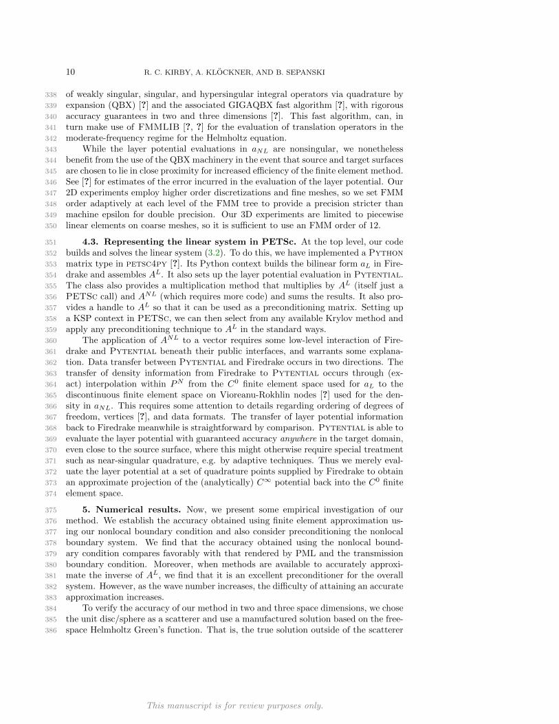
In two dimensions, we truncated the domain as the 6×6 square centered at the origin,389

shown in Figure 2 with the PML region separately highlighted. In three dimensions,390

we created an analogous mesh, the unit sphere embedded in [−3, 3]3, with the PML391

sponge region taking up [−3, 3]3 \ [−2, 2]3, shown in Figure 3.392

Fig. 2. Example 2d mesh (with PML region colored in red)

We compare our approach with transmission boundary conditions and with PML.393

Since the PML-based simulation is only accurate in the non-PML region (the blue394

region in Figure 2), we evaluate the error only over the non-PML region for all meth-395

ods, even though we solve over the entire computational domain. For computations396

with piecewise linear approximating spaces, we use affine geometry, although we use397

quadratic geometry for computations with higher-order spaces.398

We implement both PML and transmission boundary conditions in Firedrake. For399

PML, we use unbounded absorbing functions as described in [?]. This form of PML has400

no parameters to be fitted, is simple to implement in Firedrake, and has been shown401

to recover the exact solution (up to discretization errors) on annular domains [?].402

However, other implementations of PML (or equivalent boundary conditions) can403

obtain higher accuracy at lower wavelengths [?, ?].404



Fig. 3. Sample coarse 3D mesh with a spherical exclusion at the center of a cube.

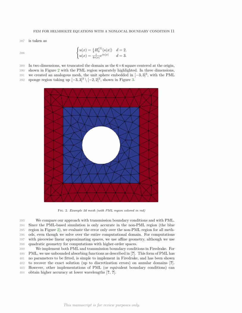
We compare the accuracy of transmission boundary conditions, PML, transmis-405

sion, and our new approach in 2D for degree 1 approximations in Figure 4. We observe406

that the transmission boundary conditions, which incur a perturbation of the PDE,407

lead to convergence to a slightly incorrect solution. Both PML and our new boundary408

conditions, however, seem to be converging to the true solution at the proper rate of409

O(h2) predicted in Theorem 2.5. For small κ, the nonlocal condition seems quite a410

bit more accurate, although they give nearly the same error for larger κ. Accuracy411

for the 2D case is reported for higher degrees in Figures 5, 6, and ?? respectively. In412

these case, we observe the theoretically-predicted convergence rates for our nonlocal413

method, although for higher degree our (suboptimal) PML does not obtain full accu-414

racy. Our theoretical results apply to 3D as well as 2D, although the computations415

are considerably more expensive. As a simple test, we have used linear polynomials416

on rather coarse meshes, presenting the results in Figure ??. We see comparable417

behavior to that obtained in 2D.418

In Figure ??, we study the error obtained versus the number of degrees of freedom419

using various orders of approximation. In these computations, we use the domain Ω′ as420

[−2, 2]2 minus the unit square and pose the boundary condition (2.10) along the outer421

boundary. Then, for each κ ∈ 0.1, 1, 5, 10 and polynomial degrees 1 through 4, we422

computed the L2 error in the numerical approximation. In addition to giving faster423

convergence rates, we also see that higher-order polynomials provide a lower error424



per degree of freedom used. Moreover, no modifications to our method or boundary425

condition were required to obtain this higher accuracy.426

10−2 10−1

10−2

10−1

100

h

Rel

ativ

eL

2E

rror

κ =0.1, degree=1

pmltransmission

nonlocal

10−2 10−1

10−2

10−1

h

Rel

ati

veL

2E

rror

κ =1.0, degree=1

pmltransmission

nonlocal

10−2 10−1

10−2

10−1

100

h

Rel

ativ

eL

2E

rror

κ =5.0, degree=1

pmltransmission

nonlocal

10−2 10−1

10−1

100

h

Rel

ativ

eL

2E

rror

κ =10.0, degree=1

pmltransmission

nonlocal

Fig. 4. L2 Relative error using degree 1 polynomials with respect to refinement in 2D. A KSPrelative tolerance of 10−12 was used. Since the transmission BC are a perturbation of the actualboundary value problem, the convergence levels off as the method converges to a slightly incorrectsolution. The PML and nonlocal methods give comparable accuracy.

We recall that our theoretical results apply to 3D as well as 2D, although the427

computations are considerably more expensive. As a simple test, we have used linear428

polynomials on rather coarse meshes, presenting the results in Figure ??. We see429

comparable behavior to that obtained in 2D.430

In Figure ??, we study the error obtained versus the number of degrees of freedom431

using various orders of approximation. In these computations, we use the domain Ω′ as432

[−2, 2]2 minus the unit square and pose the boundary condition (2.10) along the outer433

boundary. Then, for each κ ∈ 0.1, 1, 5, 10 and polynomial degrees 1 through 4, we434

computed the L2 error in the numerical approximation. In addition to giving faster435

convergence rates, we also see that higher-order polynomials provide a lower error436

per degree of freedom used. Moreover, no modifications to our method or boundary437

condition were required to obtain this higher accuracy.438

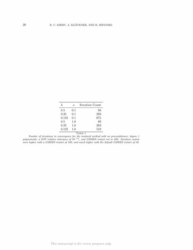
Now, we turn to efficient solution of the linear system, focusing on the two-439

dimensional case. In table 1 we see that, even for low wave numbers on coarse meshes440

with a piecewise linear discretization, solving the system without a preconditioner is441

not scalable.442

We want to demonstrate that the local part of our operator (2.4) provides an443

effective preconditioner, so that our new method can be seen as comparably difficult444

to solve as the local problem. As a first approach, we can compute a sparse LU fac-445

torization of AL to apply the inverse as a preconditioner for A. The GMRES iteration446

counts are shown in Figure ??. For a fixed κ, we see mild decrease in the iteration447



10−2 10−1

10−5

10−3

10−1

h

Rel

ati

veL

2E

rror

κ =0.1, degree=2

pmltransmission

nonlocal

10−2 10−1

10−6

10−5

10−4

10−3

10−2

10−1

h

Rel

ati

veL

2E

rror

κ =1.0, degree=2

pmltransmission

nonlocal

10−2 10−1

10−4

10−3

10−2

10−1

h

Rel

ativ

eL

2E

rror

κ =5.0, degree=2

pmltransmission

nonlocal

10−2 10−1

10−3

10−2

10−1

100

h

Rel

ativ

eL

2E

rror

κ =10.0, degree=2

pmltransmission

nonlocal

Fig. 5. L2 Relative error using degree 2 polynomials with respect to refinement in 2D. A KSPrelative tolerance of 10−12 was used.

10−1.5 10−1 10−0.510−8

10−6

10−4

10−2

100

h

Rel

ativ

eL

2E

rror

κ =0.1, degree=3

pmltransmission

nonlocal

10−1.5 10−1 10−0.5

10−7

10−5

10−3

10−1

h

Rel

ativ

eL

2E

rror

κ =1.0, degree=3

pmltransmission

nonlocal

10−1.5 10−1 10−0.510−6

10−5

10−4

10−3

10−2

10−1

h

Rel

ativ

eL

2E

rror

κ =5.0, degree=3

pmltransmission

nonlocal

10−1.5 10−1 10−0.510−5

10−4

10−3

10−2

10−1

100

h

Rel

ativ

eL

2E

rror

κ =10.0, degree=3

pmltransmission

nonlocal


count under mesh refinement. Moreover, for a fixed mesh, increasing κ corresponds448

only to a slight increase in iteration count. So, if the underlying transmission operator449



10−2 10−110−11

10−7

10−3

h

Rel

ati

veL

2E

rror

κ =0.1, degree=4

pmltransmission

nonlocal

10−1.5 10−1 10−0.510−11

10−8

10−5

10−2

h

Rel

ati

veL

2E

rror

κ =1.0, degree=4

pmltransmission

nonlocal

10−1.5 10−1 10−0.5

10−8

10−6

10−4

10−2

h

Rel

ativ

eL

2E

rror

κ =5.0, degree=4

pmltransmission

nonlocal

10−1.5 10−1 10−0.510−7

10−5

10−3

10−1

h

Rel

ativ

eL

2E

rror

κ =10.0, degree=4

pmltransmission

nonlocal


10−1 10−0.5

10−4

10−3

10−2

10−1

100

h

L2

Err

or

κ =0.1, degree=1

pmltransmission

nonlocal

10−1 10−0.5

10−3

10−2

h

L2

Err

or

κ =1.0, degree=1

pmltransmission

nonlocal

10−1 10−0.5

10−2

10−1

h

L2

Err

or

κ =5.0, degree=1

pmltransmission

nonlocal

10−1 10−0.5

10−1

10−0.5

h

L2

Err

or

κ =10.0, degree=1

pmltransmission

nonlocal

Fig. 8. L2 Error with respect to refinement in 3D using degree 1 polynomials. A KSP relativetolerance of 10−7 was used. Comparable results to Figure 4 are obtained, although we have not beenable to attain the same mesh resolutions as in 2D.



102 103 104 105 10610−11

10−8

10−5

10−2

Number of DOFs

Rel

ativ

eL

2E

rror

κ =0.1

Degree 1Degree 2Degree 3Degree 4

102 103 104 105 10610−11

10−8

10−5

10−2

Number of DOFs

Rel

ativ

eL

2E

rror

κ =1.0


102 103 104 105 106

10−8

10−5

10−2

Number of DOFs

Rel

ativ

eL

2E

rror

κ =5.0


102 103 104 105 10610−7

10−5

10−3

10−1

Number of DOFs

Rel

ativ

eL

2E

rror

κ =10.0


Fig. 9. Relative L2 error of our nonlocal method for degrees 1-4 as the number of degrees offreedom increase. A KSP relative tolerance of 10−12 was used. We used a mesh with no PMLsponge region and Σ = [−2, 2]2.

can be effectively inverted, this will in turn serve as an excellent preconditioner for450

the system with nonlocal boundary conditions. Using a direct method on AL, sparse451

factorization is typically the dominant cost. Then, each Krylov iteration requires a452

sparse matrix-vector product, an FMM evaluation, some quadrature, and solution453

with the sparse factors.454

At large enough scale, one might wish to (approximately) invert AL with an iter-455

ative method rather than factorization. To move in this direction, we used gamg [?], a456

PETSc-accessible algebraic multigrid scheme that supports complex arithmetic. This457

performed admirably at low wave number (κ . 1), but not beyond this. We were able458

to tackle higher wave numbers using the approach in [?]. The Laplacian has eigen-459

modes that become increasingly oscillatory as the eigenvalues increase. The indefinite460

Helmholtz operator shifts the eigenvalues (with the same eigenmodes) leftward in the461

complex plane. Hence, the eigenvalues closest to zero correspond to certain higher-462

frequency modes for Helmholtz. The technique in [?] approximates this oscillatory463

near null space with plane waves. To apply this method, we wrapped PyAMG [?] as a464

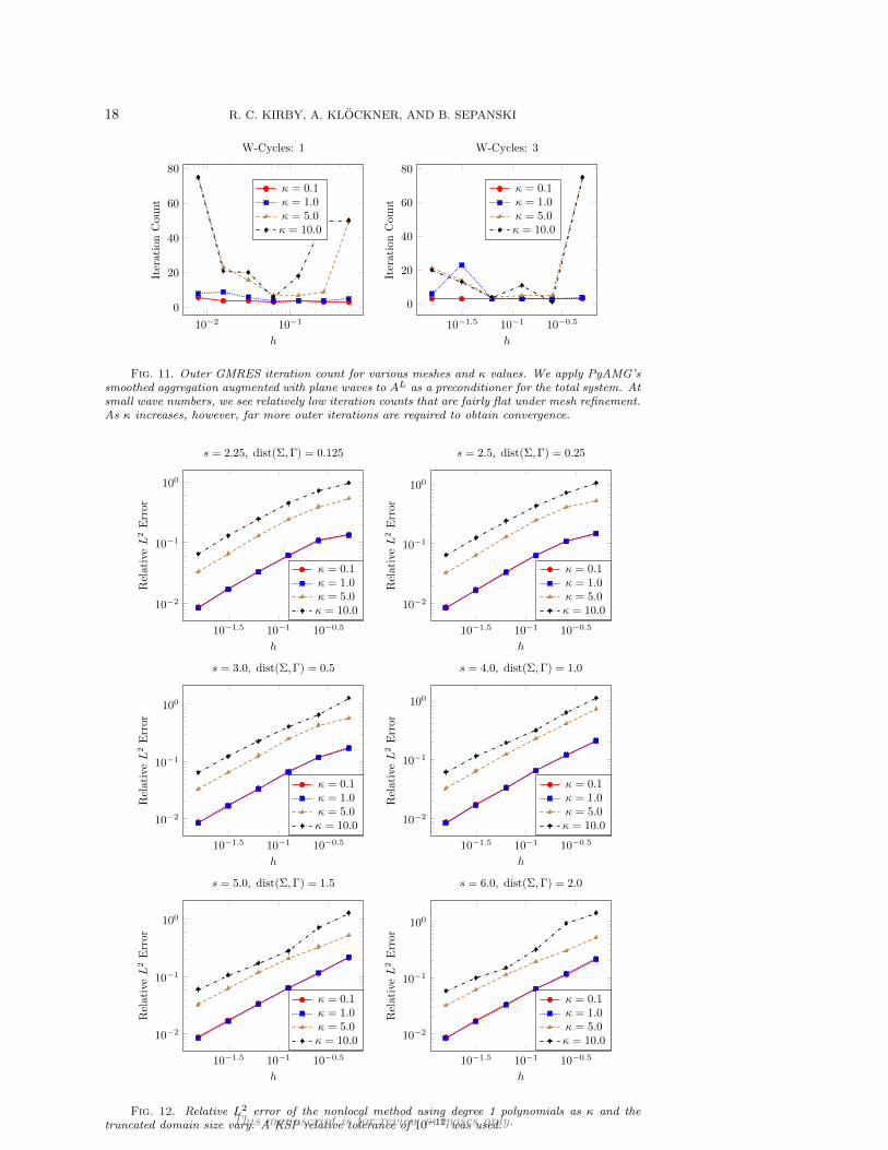
PETSc4Py preconditioner. We applied a fixed number of W-multicycles, augmented465

with plane waves in the same way as in [?], to AL as a preconditioner for the overall466

system. Figure ?? shows the results we obtained. The preconditioner is very effective467

at low κ but requires more iterations for larger ones. However, we see that applying468

more W-cycles within the preconditioner typically leads to a lower outer iteration469



10−2 10−1

4

5

6

7

h

Iter

atio

nN

um

ber

degree=1

κ =0.1κ =1.0κ =5.0κ =10.0

10−2 10−1

4

5

6

7

8

h

Iter

atio

nN

um

ber

degree=2

κ =0.1κ =1.0κ =5.0κ =10.0

10−1.5 10−1 10−0.5

3

4

5

6

7

h

Iter

atio

nN

um

ber

degree=3

κ =0.1κ =1.0κ =5.0κ =10.0

10−2 10−1

3

4

5

6

7

h

Iter

ati

onN

um

ber

degree=4

κ =0.1κ =1.0κ =5.0κ =10.0

Fig. 10. GMRES iteration counts for a two-dimensional mesh using LU factorization for AL

as a preconditioner for various values of κ. Fixing κ and refining the mesh (right to left) leads to aslight decrease in iteration count, while fixing a mesh and increasing κ leads to a mild increase initeration count.

count. Comparing Figure ?? to Figure ?? suggests that the difference in iteration470

counts follows from the difficulty in obtaining an effective iterative method for the471

regular Helmholtz operator rather than new difficulties presented by our nonlocal472

boundary condition.473

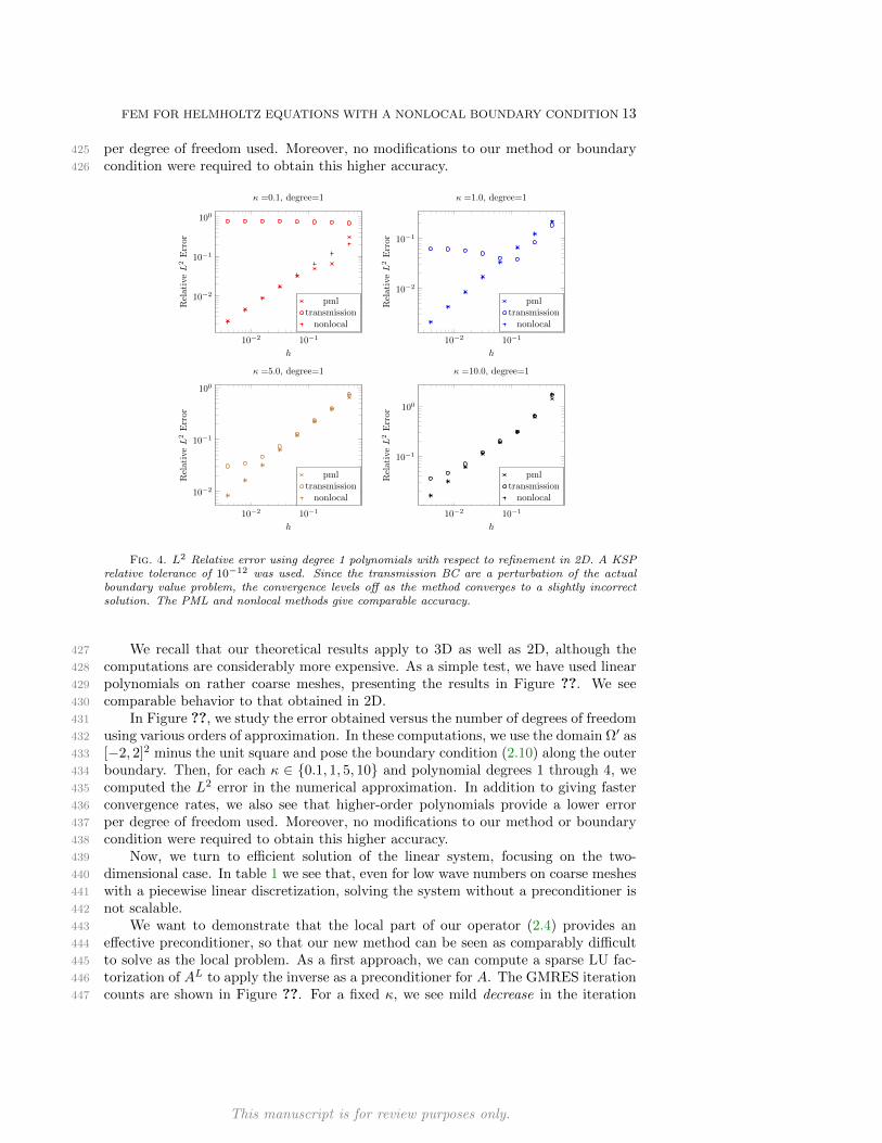
Finally, we devise an experiment to demonstrate our method’s robustness with474

respect to the distance between the scatterer boundary Γ and the truncated boundary475

Σ. We continue to use the circle of radius 1 centered at the origin as the scatter Γ.476

For side length s ∈ 2.25, 2.5, 3.0, 4.0, 5.0, 6.0, we truncated the domain as the square477

[− s2 ,s2 ]2 take out the circle of radius 1. In Figure ??, we measure the relative L2 error478

of our nonlocal method for each domain. We see no pathologies emerging as the479

computational domain becomes smaller.480



10−2 10−1

0

20

40

60

80

h

Iter

atio

nC

ount

W-Cycles: 1

κ = 0.1κ = 1.0κ = 5.0κ = 10.0

10−1.5 10−1 10−0.5

0

20

40

60

80

h

Iter

atio

nC

ou

nt

W-Cycles: 3

κ = 0.1κ = 1.0κ = 5.0κ = 10.0

Fig. 11. Outer GMRES iteration count for various meshes and κ values. We apply PyAMG’ssmoothed aggregation augmented with plane waves to AL as a preconditioner for the total system. Atsmall wave numbers, we see relatively low iteration counts that are fairly flat under mesh refinement.As κ increases, however, far more outer iterations are required to obtain convergence.

10−1.5 10−1 10−0.5

10−2

10−1

100

h

Rel

ativ

eL

2E

rror

s = 2.25, dist(Σ,Γ) = 0.125

κ = 0.1κ = 1.0κ = 5.0κ = 10.0

10−1.5 10−1 10−0.5

10−2

10−1

100

h

Rel

ativ

eL

2E

rror

s = 2.5, dist(Σ,Γ) = 0.25

κ = 0.1κ = 1.0κ = 5.0κ = 10.0

10−1.5 10−1 10−0.5

10−2

10−1

100

h

Rel

ativ

eL

2E

rror

s = 3.0, dist(Σ,Γ) = 0.5

κ = 0.1κ = 1.0κ = 5.0κ = 10.0

10−1.5 10−1 10−0.5

10−2

10−1

100

h

Rel

ativ

eL

2E

rror

s = 4.0, dist(Σ,Γ) = 1.0

κ = 0.1κ = 1.0κ = 5.0κ = 10.0

10−1.5 10−1 10−0.5

10−2

10−1

100

h

Rel

ativ

eL

2E

rror

s = 5.0, dist(Σ,Γ) = 1.5

κ = 0.1κ = 1.0κ = 5.0κ = 10.0

10−1.5 10−1 10−0.5

10−2

10−1

100

h

Rel

ativ

eL

2E

rror

s = 6.0, dist(Σ,Γ) = 2.0

κ = 0.1κ = 1.0κ = 5.0κ = 10.0

Fig. 12. Relative L2 error of the nonlocal method using degree 1 polynomials as κ and thetruncated domain size vary. A KSP relative tolerance of 10−12 was used.This manuscript is for review purposes only.


6. Conclusions and future work. We have proposed a new nonlocal boundary481

condition for exterior Helmholtz problems. This condition, based on Green’s formula482

and expressed in terms of layer potentials, works in general unstructured geometry483

in two and three dimensions. Thanks to a Garding inequality, we have optimal finite484

element error estimates under standard conditions. The nonlocal terms are amenable485

to approximation by fast multipole expansions, and the discrete system can be readily486

preconditioned by its local part. In the future, it should be possible to extend the487

analysis to handle inexactness in evaluating the boundary terms. Moreover, we antic-488

ipate being able to apply this technique to a much broader class of problems such as489

exterior curl-curl problems. Additionally, we are working to integrate layer potentials490

with Firedrake’s top-level language to make it easier to apply the method.491



h κ Iteration Count

0.5 0.1 880.25 0.1 2930.125 0.1 6750.5 1.0 890.25 1.0 2830.125 1.0 519

Table 1Number of iterations to convergence for the nonlocal method with no preconditioner, degree 1

polynomials, a KSP relative tolerance of 10−12, and GMRES restart set to 200. Iteration countswere higher with a GMRES restart of 100, and much higher with the default GMRES restart of 30.


finite elements for helmholtz equations with a nonlocal

Documents