olivier pierre-louis, ilm-lyon - sciencesconf.org · 2017-06-20 · olivier pierre-louis (ilm-lyon,...
TRANSCRIPT
Olivier Pierre-Louis, ILM-Lyon
Olivier Pierre-Louis (ILM-Lyon, France.) Lecture 1: Non-equilibrium interface dynamics in crystal growth 27th May 2017 1 / 92
XXIme ”Aux Rencontres de Peyresq”
Dynamiques et Instabilites d’interfaceEcole thematique d’ete, 29/05 to 2/06 2017
3 lectures:
Non-equilibrium & nonlinear dynamics of interfaces in growth
Thin films – dewetting – solid-state
Membranes - adhesion and confinement
Leitmotiv:
Modelling non-equilibrium interfaces
Nonlinear phenomena, instabilities, morphology
Olivier Pierre-Louis (ILM-Lyon, France.) Lecture 1: Non-equilibrium interface dynamics in crystal growth 27th May 2017 2 / 92
Lecture 1: Non-equilibrium interface dynamics in crystal growth
Olivier Pierre-Louis
ILM-Lyon, France.
27th May 2017
Olivier Pierre-Louis (ILM-Lyon, France.) Lecture 1: Non-equilibrium interface dynamics in crystal growth 27th May 2017 3 / 92
1 IntroductionModels and levels of descriptionAtomic steps and surface dynamics
2 Kinetic Monte CarloMaster EquationKMC algorithmKMC Simulations
3 Phase field modelsDiffuse interfaces modelsAsympoticsPhase field simualtions
4 BCF Step modelBurton-Cabrera-Frank step modelMulti-scale analysis
5 Nonlinear interface dynamicsPreamble in 0DNonlinear dynamics in 1D
6 Conclusion
Olivier Pierre-Louis (ILM-Lyon, France.) Lecture 1: Non-equilibrium interface dynamics in crystal growth 27th May 2017 4 / 92
Introduction
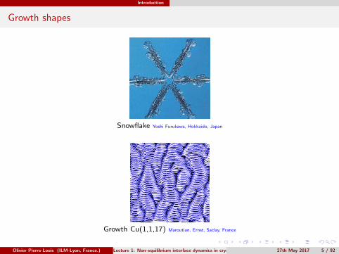
Growth shapes
Snowflake Yoshi Furukawa, Hokkaido, Japan
Growth Cu(1,1,17) Maroutian, Ernst, Saclay, France
Olivier Pierre-Louis (ILM-Lyon, France.) Lecture 1: Non-equilibrium interface dynamics in crystal growth 27th May 2017 5 / 92
Introduction Models and levels of description
Contents
1 IntroductionModels and levels of descriptionAtomic steps and surface dynamics
2 Kinetic Monte CarloMaster EquationKMC algorithmKMC Simulations
3 Phase field modelsDiffuse interfaces modelsAsympoticsPhase field simualtions
4 BCF Step modelBurton-Cabrera-Frank step modelMulti-scale analysis
5 Nonlinear interface dynamicsPreamble in 0DNonlinear dynamics in 1D
6 Conclusion
Olivier Pierre-Louis (ILM-Lyon, France.) Lecture 1: Non-equilibrium interface dynamics in crystal growth 27th May 2017 6 / 92
Introduction Models and levels of description
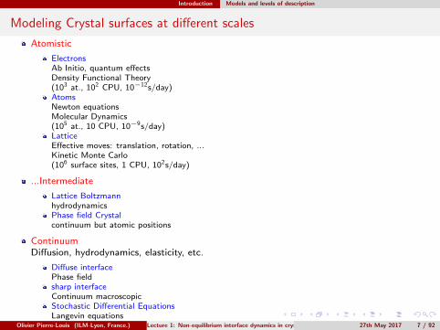
Modeling Crystal surfaces at different scales
Atomistic
ElectronsAb Initio, quantum effectsDensity Functional Theory(103 at., 102 CPU, 10−12s/day)AtomsNewton equationsMolecular Dynamics(105 at., 10 CPU, 10−9s/day)LatticeEffective moves: translation, rotation, ...Kinetic Monte Carlo(106 surface sites, 1 CPU, 102s/day)
...Intermediate
Lattice BoltzmannhydrodynamicsPhase field Crystalcontinuum but atomic positions
ContinuumDiffusion, hydrodynamics, elasticity, etc.
Diffuse interfacePhase fieldsharp interfaceContinuum macroscopicStochastic Differential EquationsLangevin equations
Olivier Pierre-Louis (ILM-Lyon, France.) Lecture 1: Non-equilibrium interface dynamics in crystal growth 27th May 2017 7 / 92
Introduction Models and levels of description
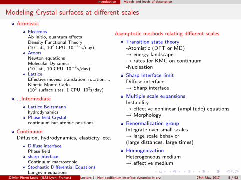
Modeling Crystal surfaces at different scales
Atomistic
ElectronsAb Initio, quantum effectsDensity Functional Theory(103 at., 102 CPU, 10−12s/day)AtomsNewton equationsMolecular Dynamics(105 at., 10 CPU, 10−9s/day)LatticeEffective moves: translation, rotation, ...Kinetic Monte Carlo(106 surface sites, 1 CPU, 102s/day)
...Intermediate
Lattice BoltzmannhydrodynamicsPhase field Crystalcontinuum but atomic positions
ContinuumDiffusion, hydrodynamics, elasticity, etc.
Diffuse interfacePhase fieldsharp interfaceContinuum macroscopicStochastic Differential EquationsLangevin equations
Asymptotic methods relating different scales
Transition state theory-Atomistic (DFT or MD)→ energy landscape→ rates for KMC on continuum-Nucleation
Sharp interface limitDiffuse interface→ Sharp interface
Multiple scale expansionsInstability→ effective nonlinear (amplitude) equations→ Morphology
Renormalization groupIntegrate over small scales→ large scale behavior(large distances, large times)
HomogenizationHeterogeneous medium→ effective medium
Olivier Pierre-Louis (ILM-Lyon, France.) Lecture 1: Non-equilibrium interface dynamics in crystal growth 27th May 2017 8 / 92

Introduction Models and levels of description
Direct derivation Vs. Asymptotic analysis
Atomistic
ElectronsAb Initio, quantum effectsDensity Functional Theory(103 at., 102 CPU, 10−12s/day)AtomsNewton equationsMolecular Dynamics(105 at., 10 CPU, 10−9s/day)LatticeEffective moves: translation, rotation, etc.Kinetic Monte Carlo(106 surface sites, 1 CPU, 102s/day)
...Intermediate
Lattice BoltzmannhydrodynamicsPhase field Crystalcontinuum but atomic positions
ContinuumDiffusion, hydrodynamics, elasticity, etc.
Diffuse interfacePhase fieldsharp interfaceContinuum macroscopicStochastic Differential EquationsLangevin equations
Direct derivation of models(phenomenological models)
Symmetries
Conservation Laws
Linear Irreversible Thermodynamics(Onsager)
... etc.
Olivier Pierre-Louis (ILM-Lyon, France.) Lecture 1: Non-equilibrium interface dynamics in crystal growth 27th May 2017 9 / 92
Introduction Atomic steps and surface dynamics
Contents
1 IntroductionModels and levels of descriptionAtomic steps and surface dynamics
2 Kinetic Monte CarloMaster EquationKMC algorithmKMC Simulations
3 Phase field modelsDiffuse interfaces modelsAsympoticsPhase field simualtions
4 BCF Step modelBurton-Cabrera-Frank step modelMulti-scale analysis
5 Nonlinear interface dynamicsPreamble in 0DNonlinear dynamics in 1D
6 Conclusion
Olivier Pierre-Louis (ILM-Lyon, France.) Lecture 1: Non-equilibrium interface dynamics in crystal growth 27th May 2017 10 / 92
Introduction Atomic steps and surface dynamics
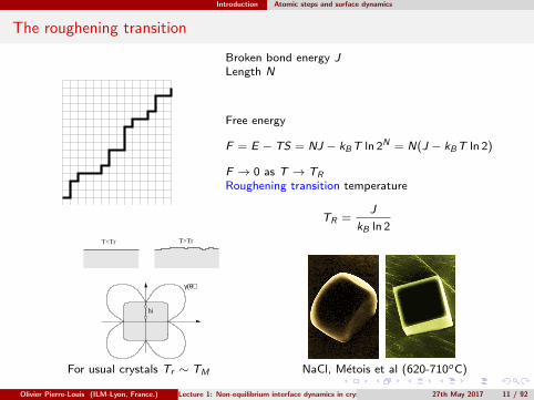
The roughening transition
Broken bond energy JLength N
Free energy
F = E − TS = NJ − kBT ln 2N = N(J − kBT ln 2)
F → 0 as T → TR
Roughening transition temperature
TR =J
kB ln 2
γ(θ)
T<Tr T>Tr.
hi
For usual crystals Tr ∼ TM NaCl, Metois et al (620-710oC)
Olivier Pierre-Louis (ILM-Lyon, France.) Lecture 1: Non-equilibrium interface dynamics in crystal growth 27th May 2017 11 / 92

Introduction Atomic steps and surface dynamics
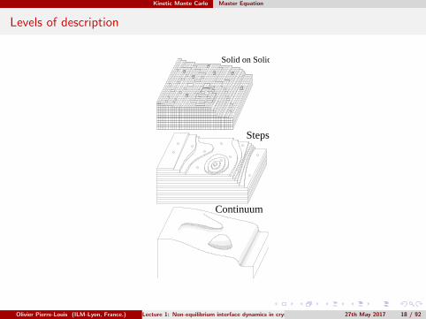
Levels of description
Solid on Solid
Steps
Continuum
Olivier Pierre-Louis (ILM-Lyon, France.) Lecture 1: Non-equilibrium interface dynamics in crystal growth 27th May 2017 12 / 92

Introduction Atomic steps and surface dynamics
Atomic steps
Si(100)
M. Lagally, Univ. Visconsin
Insulin
P. Vekilov, Houston
Olivier Pierre-Louis (ILM-Lyon, France.) Lecture 1: Non-equilibrium interface dynamics in crystal growth 27th May 2017 13 / 92

Introduction Atomic steps and surface dynamics
Nano-scale Relaxation
Ag(111), Sintering
M. Giesen, Julich Germany
Decay Cu(1,1,1) 10mM HCl at (a) -580mV; and (b) 510 mV
Broekman et al, (1999) J. Electroanal. Chem.
Olivier Pierre-Louis (ILM-Lyon, France.) Lecture 1: Non-equilibrium interface dynamics in crystal growth 27th May 2017 14 / 92
Introduction Atomic steps and surface dynamics
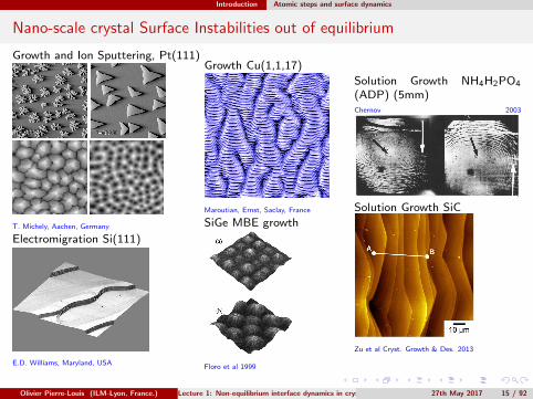
Nano-scale crystal Surface Instabilities out of equilibrium
Growth and Ion Sputtering, Pt(111)
T. Michely, Aachen, Germany
Electromigration Si(111)
E.D. Williams, Maryland, USA
Growth Cu(1,1,17)
Maroutian, Ernst, Saclay, France
SiGe MBE growth
Floro et al 1999
Solution Growth NH4H2PO4
(ADP) (5mm)Chernov 2003
Solution Growth SiC
Zu et al Cryst. Growth & Des. 2013
Olivier Pierre-Louis (ILM-Lyon, France.) Lecture 1: Non-equilibrium interface dynamics in crystal growth 27th May 2017 15 / 92
Introduction Atomic steps and surface dynamics
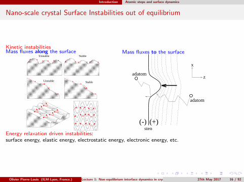
Nano-scale crystal Surface Instabilities out of equilibrium
Kinetic instabilitiesMass fluxes along the surface
Unstable
Unstable
Stable
Stable
Mass fluxes to the surface
adatomz
x
(+)(-)step
adatom
Energy relaxation driven instabilities:surface energy, elastic energy, electrostatic energy, electronic energy, etc.
Olivier Pierre-Louis (ILM-Lyon, France.) Lecture 1: Non-equilibrium interface dynamics in crystal growth 27th May 2017 16 / 92
Kinetic Monte Carlo Master Equation
Contents
1 IntroductionModels and levels of descriptionAtomic steps and surface dynamics
2 Kinetic Monte CarloMaster EquationKMC algorithmKMC Simulations
3 Phase field modelsDiffuse interfaces modelsAsympoticsPhase field simualtions
4 BCF Step modelBurton-Cabrera-Frank step modelMulti-scale analysis
5 Nonlinear interface dynamicsPreamble in 0DNonlinear dynamics in 1D
6 Conclusion
Olivier Pierre-Louis (ILM-Lyon, France.) Lecture 1: Non-equilibrium interface dynamics in crystal growth 27th May 2017 17 / 92
Kinetic Monte Carlo Master Equation
Levels of description
Solid on Solid
Steps
Continuum
Olivier Pierre-Louis (ILM-Lyon, France.) Lecture 1: Non-equilibrium interface dynamics in crystal growth 27th May 2017 18 / 92
Kinetic Monte Carlo Master Equation
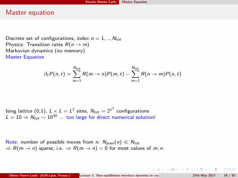
Master equation
Discrete set of configurations, index n = 1, ..,Ntot
Physics: Transition rates R(n→ m)Markovian dynamics (no memory)Master Equation
∂tP(n, t) =
Ntot∑m=1
R(m→ n)P(m, t)−Ntot∑m=1
R(n→ m)P(n, t)
Ising lattice (0,1), L× L = L2 sites, Ntot = 2L2
configurationsL = 10⇒ Ntot ∼ 1030 ... too large for direct numerical solution!
Note: number of possible moves from n: Nposs(n) Ntot
⇒ R(m→ n) sparse, i.e. ⇒ R(m→ n) = 0 for most values of m, n.
Olivier Pierre-Louis (ILM-Lyon, France.) Lecture 1: Non-equilibrium interface dynamics in crystal growth 27th May 2017 19 / 92
Kinetic Monte Carlo Master Equation
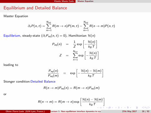
Equilibrium and Detailed Balance
Master Equation
∂tP(n, t) =
Ntot∑m=1
R(m→ n)P(m, t)−Ntot∑m=1
R(n→ m)P(n, t)
Equilibrium, steady-state (∂tPeq(n, t) = 0), Hamiltonian H(n)
Peq(n) =1
Zexp
[−H(n)
kBT
]
Z =
Ntot∑n=1
exp
[−H(n)
kBT
]leading to
Peq(n)
Peq(m)= exp
[−H(n)−H(m)
kBT
]Stonger condition:Detailed Balance
R(n→ m)Peq(n) = R(m→ n)Peq(m)
or
R(n→ m) = R(m→ n) exp
[H(n)−H(m)
kBT
]Olivier Pierre-Louis (ILM-Lyon, France.) Lecture 1: Non-equilibrium interface dynamics in crystal growth 27th May 2017 20 / 92

Kinetic Monte Carlo Master Equation
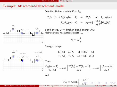
Example : Attachment-Detachment model
i
r(hi −> hi+1)
r(hi −> hi−1)
i
i
hi
n =1
n =2n =3
i
ii
(b)
(c)
(a)
State n = hi ; i = 1.., LRates
R(hi → hi + 1) = F
R(hi → hi − 1) = r0 exp[−niJ
kBT]
ni number nearest neighbors at site i before detachment(Breaking all bonds to detach / Transition state Theory)
Feq = r0 exp
[−
2J
kBT
]
Olivier Pierre-Louis (ILM-Lyon, France.) Lecture 1: Non-equilibrium interface dynamics in crystal growth 27th May 2017 21 / 92
Kinetic Monte Carlo Master Equation
Example: Attachment-Detachment model
i
n =1
n =2n =3
i
ii
i
n =1
n =2n =3
ii
i
Ls −> Ls−2
Ls −> Ls+2
Ls −> Ls
Detailed Balance when F = Feq
R(hi − 1→ hi )Peq(hi − 1) = R(hi → hi − 1)Peq(hi )
FeqPeq(hi − 1) = r0 exp[−niJ
kBT]Peq(hi )
Bond energy J ⇒ Broken Bond energy J/2Hamiltonian H, surface length Ls
H = LsJ
2
Energy change
Ls(hi )− Ls(hi − 1) = 2(2− ni )
H(hi )−H(hi − 1) = (2− ni )J
Thus
Peq(hi − 1)
Peq(hi )= exp
[H(hi )−H(hi − 1)
kBT
]= exp
[(2− ni )J
kBT
]and
Feq = r0 exp
[−
2J
kBT
]Olivier Pierre-Louis (ILM-Lyon, France.) Lecture 1: Non-equilibrium interface dynamics in crystal growth 27th May 2017 22 / 92
Kinetic Monte Carlo Master Equation
Example: Attachment-Detachment model
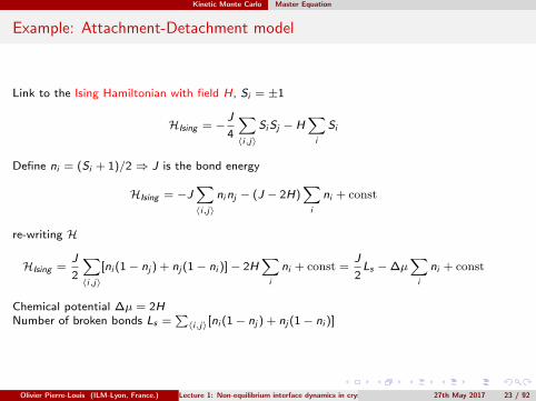
Link to the Ising Hamiltonian with field H, Si = ±1
HIsing = −J
4
∑〈i,j〉
SiSj − H∑i
Si
Define ni = (Si + 1)/2 ⇒ J is the bond energy
HIsing = −J∑〈i,j〉
ninj − (J − 2H)∑i
ni + const
re-writing H
HIsing =J
2
∑〈i,j〉
[ni (1− nj ) + nj (1− ni )]− 2H∑i
ni + const =J
2Ls −∆µ
∑i
ni + const
Chemical potential ∆µ = 2HNumber of broken bonds Ls =
∑〈i,j〉[ni (1− nj ) + nj (1− ni )]
Olivier Pierre-Louis (ILM-Lyon, France.) Lecture 1: Non-equilibrium interface dynamics in crystal growth 27th May 2017 23 / 92
Kinetic Monte Carlo Master Equation
Example: Attachment-Detachment model
Chemical potential ∆µ = 2HDetailed Balance imposed to the Ising system with field H
F = R(hi − 1→ hi ) = R(hi → hi − 1)P Isingeq (hi )
P Isingeq (hi − 1)
= exp
[−niJ +HIsing (hi )−HIsing (hi − 1)
kBT
]= exp
[−
niJ
kBT+
[Ls(hi )− Ls(hi − 1)]J
2kBT+
∆µ
kBT
]= exp
[−
niJ
kBT+
2(ni − 2)J
2kBT+
∆µ
kBT
]= Feq exp
[∆µ
kBT
]
Feq = r0 exp
[−
2J
kBT
]Attachement-Detachment model equivalent to Ising in Magnetic field
Olivier Pierre-Louis (ILM-Lyon, France.) Lecture 1: Non-equilibrium interface dynamics in crystal growth 27th May 2017 24 / 92
Kinetic Monte Carlo Master Equation
Equilibrium Monte Carlo: Metropolis algorithm
Algorithm
1 Choose an event n→ m at random
2 implement the event with probability
H(n) ≥ H(m) ⇒ P(n→ m) = 1
H(n) ≤ H(m) ⇒ P(n→ m) = exp[−H(m)−H(n)
kBT]
Obeys Detailed Balance
R(n→ m)
R(m→ n)= exp
[−H(n)−H(m)
kBT
]Chain of events conv. to equil. ⇒ sample configuration space n ⇒ Thermodynamic averagesNo time!
Olivier Pierre-Louis (ILM-Lyon, France.) Lecture 1: Non-equilibrium interface dynamics in crystal growth 27th May 2017 25 / 92
Kinetic Monte Carlo KMC algorithm
Contents
1 IntroductionModels and levels of descriptionAtomic steps and surface dynamics
2 Kinetic Monte CarloMaster EquationKMC algorithmKMC Simulations
3 Phase field modelsDiffuse interfaces modelsAsympoticsPhase field simualtions
4 BCF Step modelBurton-Cabrera-Frank step modelMulti-scale analysis
5 Nonlinear interface dynamicsPreamble in 0DNonlinear dynamics in 1D
6 Conclusion
Olivier Pierre-Louis (ILM-Lyon, France.) Lecture 1: Non-equilibrium interface dynamics in crystal growth 27th May 2017 26 / 92

Kinetic Monte Carlo KMC algorithm
A simple Monte Carlo method with time: random attempts
Using physical rates R(n→ m) from a given model
Algorithm
1 Choose an event n→ m at random
2 Implement the event with probability
P(n→ m) =R(n→ m)
Rmax
where Rmax = maxn′ (R(n→ n′)).
3 implement the time by ∆t ∼ 1/(Nposs(n)Rmax )Nposs(n) number of possible moves from state n
Problem: when most R(n→ m) Rmax , then most P(n→ m) 1 ⇒ most attempts rejected!
Questions
a rejection-free algorithm?
time implementation?
Olivier Pierre-Louis (ILM-Lyon, France.) Lecture 1: Non-equilibrium interface dynamics in crystal growth 27th May 2017 27 / 92

Kinetic Monte Carlo KMC algorithm
Kinetic Monte Carlo algorithm 1: Rejection-free algorithm
implement the FIRST event that occurs
Probability first chosen event n→ m is ∼ R(n→ m)
Choose event with probability
P(n→ m) =R(n→ m)
Rtot(n)
Rate that one event occurs
Rtot(n) =
Ntot∑m=1
R(n→ m)
Algorithm
1 Build cumulative rates Rc (m) =∑m
p=1 R(n→ p), with
Rc (Ntot) = Rtot(n).
2 Choose random number Rrand , uniformly distributed with0 < Rrand ≤ Rtot(n).
3 Choose event n∗ such that Rc (n∗ − 1) < Rrand ≤ Rc (n∗).
0
Rc(1)
Rc(3)
Rc(4)
Rc(7)
Rc(8)
Rc(9)Rc(10)
Rc(5)Rc(6)
0
Rc(2)
Rrand
.
n*=5
Rc(10)
Olivier Pierre-Louis (ILM-Lyon, France.) Lecture 1: Non-equilibrium interface dynamics in crystal growth 27th May 2017 28 / 92
Kinetic Monte Carlo KMC algorithm
Kinetic Monte Carlo algorithm 3: comments
Algorithm
1 Build cumulative rates Rc (m) =∑m
p=1 R(n→ p), with Rc (Ntot) = Rtot(n).
2 Choose random number Rrand , uniformly distributed with 0 < Rrand ≤ Rtot(n).
3 Choose event n∗ such that Rc (n∗ − 1) < Rrand ≤ Rc (n∗).
Improved algorithm:
Number of possible events from one state Nposs(n) number of states Ntot(n)
Groups of events with same rates
Olivier Pierre-Louis (ILM-Lyon, France.) Lecture 1: Non-equilibrium interface dynamics in crystal growth 27th May 2017 29 / 92
Kinetic Monte Carlo KMC algorithm
Kinetic Monte Carlo algorithm 2: implementing time
Define τ time with τ = 0 when arriving in state nProba Q(τ) that no event occurs up to time τ , with Q(0) = 1
Q(τ + dτ) = Q(τ)(1− Rtot(n)dτ)⇒dQ(τ)
dτ= −Rtot(n)Q(τ)⇒ Q(τ) = exp[−Rtot(n)τ ]
probability density ρ, i.e. ρ(τ)dτ first event occuring between τ and τ + dτ
ρ(τ)dτ = −dQ(τ) = Rtot(n) exp[−Rtot(n)τ ]dτ
Easy to generate: uniform distribution ρ(u) = 1, and 0 < u ≤ 1Variable change
u = exp[−Rtot(n)τ ]
same probability density
ρ(τ)dτ = −ρ(u)du
Algorithm
1 Choose random number u, uniformly distributed with 0 < u ≤ 1.
2 Time increment t → t + τ with
τ =− log(u)
Rtot(n)
Olivier Pierre-Louis (ILM-Lyon, France.) Lecture 1: Non-equilibrium interface dynamics in crystal growth 27th May 2017 30 / 92

Kinetic Monte Carlo KMC Simulations
Contents
1 IntroductionModels and levels of descriptionAtomic steps and surface dynamics
2 Kinetic Monte CarloMaster EquationKMC algorithmKMC Simulations
3 Phase field modelsDiffuse interfaces modelsAsympoticsPhase field simualtions
4 BCF Step modelBurton-Cabrera-Frank step modelMulti-scale analysis
5 Nonlinear interface dynamicsPreamble in 0DNonlinear dynamics in 1D
6 Conclusion
Olivier Pierre-Louis (ILM-Lyon, France.) Lecture 1: Non-equilibrium interface dynamics in crystal growth 27th May 2017 31 / 92
Kinetic Monte Carlo KMC Simulations
Attachment-detachment model
10−4
10−2
10 0
10 2
10 4
10−2 10 0 10 2 10 4
Acl
(t)
/ A
cl (
0)
a0 ν0 t / R0
∆µ /J
0−0.05
+0.05
(a)
F = Feqe−∆µ/kBT
Saito, Pierre-Louis, PRL 2012
Olivier Pierre-Louis (ILM-Lyon, France.) Lecture 1: Non-equilibrium interface dynamics in crystal growth 27th May 2017 32 / 92
Kinetic Monte Carlo KMC Simulations
Nano-scale crystal Surface Instabilities out of equilibrium
Movie...
Olivier Pierre-Louis (ILM-Lyon, France.) Lecture 1: Non-equilibrium interface dynamics in crystal growth 27th May 2017 33 / 92
Kinetic Monte Carlo KMC Simulations
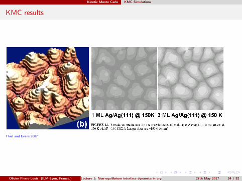
KMC results
Thiel and Evans 2007
Olivier Pierre-Louis (ILM-Lyon, France.) Lecture 1: Non-equilibrium interface dynamics in crystal growth 27th May 2017 34 / 92

Kinetic Monte Carlo KMC Simulations
KMC vs SOI solid-state dewetting
h = 3, ES = 1, T = 0.5
E. Bussman, F. Leroy, F. Cheynis, P. Muller, O. Pierre-Louis NJP 2011
Olivier Pierre-Louis (ILM-Lyon, France.) Lecture 1: Non-equilibrium interface dynamics in crystal growth 27th May 2017 35 / 92
Kinetic Monte Carlo KMC Simulations
KMC conclusion
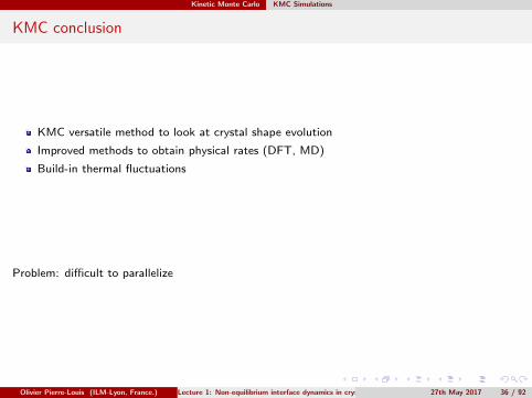
KMC versatile method to look at crystal shape evolution
Improved methods to obtain physical rates (DFT, MD)
Build-in thermal fluctuations
Problem: difficult to parallelize
Olivier Pierre-Louis (ILM-Lyon, France.) Lecture 1: Non-equilibrium interface dynamics in crystal growth 27th May 2017 36 / 92

Kinetic Monte Carlo KMC Simulations
Step meandering Instabilities
Non-equilibrium meandering of a stepSchwoebel effect + terrace diffusionBales and Zangwill 1990
adatomz
x
(+)(-)step
adatom
Y. Saito, M. Uwaha 1994
Solving step dynamics→ morphology and coupling to a diffusion field
Olivier Pierre-Louis (ILM-Lyon, France.) Lecture 1: Non-equilibrium interface dynamics in crystal growth 27th May 2017 37 / 92

Phase field models Diffuse interfaces models
Contents
1 IntroductionModels and levels of descriptionAtomic steps and surface dynamics
2 Kinetic Monte CarloMaster EquationKMC algorithmKMC Simulations
3 Phase field modelsDiffuse interfaces modelsAsympoticsPhase field simualtions
4 BCF Step modelBurton-Cabrera-Frank step modelMulti-scale analysis
5 Nonlinear interface dynamicsPreamble in 0DNonlinear dynamics in 1D
6 Conclusion
Olivier Pierre-Louis (ILM-Lyon, France.) Lecture 1: Non-equilibrium interface dynamics in crystal growth 27th May 2017 38 / 92
Phase field models Diffuse interfaces models
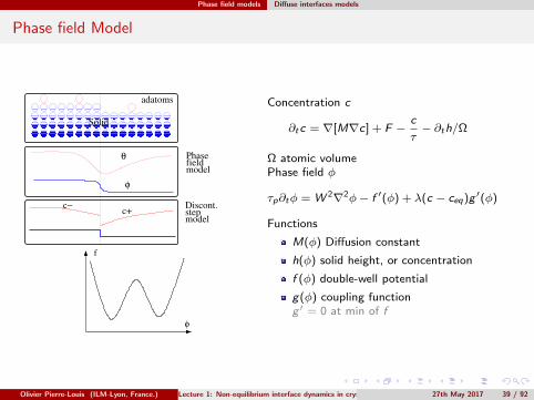
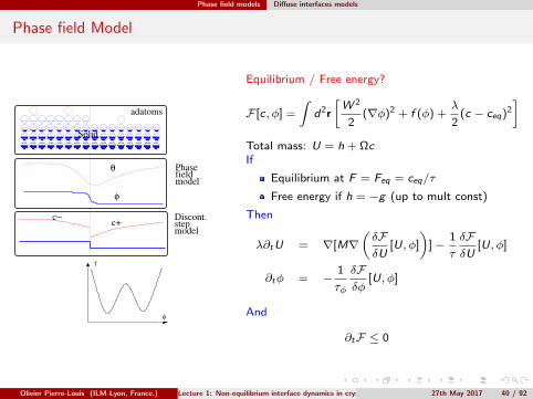
Phase field Model
adatoms
Solid
c+c−
θ
φ
Phasefieldmodel
stepmodel
.
Discont.
φ
f
Concentration c
∂tc = ∇[M∇c] + F −c
τ− ∂th/Ω
Ω atomic volumePhase field φ
τp∂tφ = W 2∇2φ− f ′(φ) + λ(c − ceq)g ′(φ)
Functions
M(φ) Diffusion constant
h(φ) solid height, or concentration
f (φ) double-well potential
g(φ) coupling functiong ′ = 0 at min of f
Olivier Pierre-Louis (ILM-Lyon, France.) Lecture 1: Non-equilibrium interface dynamics in crystal growth 27th May 2017 39 / 92
Phase field models Diffuse interfaces models
Phase field Model
adatoms
Solid
c+c−
θ
φ
Phasefieldmodel
stepmodel
.
Discont.
φ
f
Equilibrium / Free energy?
F [c, φ] =
∫d2r
[W 2
2(∇φ)2 + f (φ) +
λ
2(c − ceq)2
]Total mass: U = h + ΩcIf
Equilibrium at F = Feq = ceq/τ
Free energy if h = −g (up to mult const)
Then
λ∂tU = ∇[M∇(δFδU
[U, φ]
)]−
1
τ
δFδU
[U, φ]
∂tφ = −1
τφ
δFδφ
[U, φ]
And
∂tF ≤ 0
Olivier Pierre-Louis (ILM-Lyon, France.) Lecture 1: Non-equilibrium interface dynamics in crystal growth 27th May 2017 40 / 92
Phase field models Asympotics
Contents
1 IntroductionModels and levels of descriptionAtomic steps and surface dynamics
2 Kinetic Monte CarloMaster EquationKMC algorithmKMC Simulations
3 Phase field modelsDiffuse interfaces modelsAsympoticsPhase field simualtions
4 BCF Step modelBurton-Cabrera-Frank step modelMulti-scale analysis
5 Nonlinear interface dynamicsPreamble in 0DNonlinear dynamics in 1D
6 Conclusion
Olivier Pierre-Louis (ILM-Lyon, France.) Lecture 1: Non-equilibrium interface dynamics in crystal growth 27th May 2017 41 / 92

Phase field models Asympotics
Asymptotic expansion
d
W
s(out)
(in)
interface
ε ∼W /`c ; η = d/ε; ∇d = n
Two expansions: ”inner domain” and ”outer domain”
c in(η, s, t) =∞∑n=0
εnc inn (η, s, t)
cout(x , y , t) =∞∑n=0
εncoutn (x , y , t)
Matching conditions c in(η) = cout(εη)with η →∞, ε→ 0, εη → 0
limη→±∞
c in0 = limd→0±
cout0
limη→±∞
∂ηcin0 = 0
limη→±∞
c in1 = limd→0±
cout1 + η limd→0±
n.∇cout0
limη→±∞
∂ηcin1 = lim
d→0±n.∇cout0
limη→±∞
∂ηηcin1 = 0
Olivier Pierre-Louis (ILM-Lyon, France.) Lecture 1: Non-equilibrium interface dynamics in crystal growth 27th May 2017 42 / 92
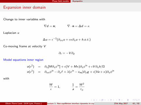
Phase field models Asympotics
Expansion inner domain
Change to inner variables with
∇d = n; ∇ · n = ∆d = κ
Laplacian u
∆u = ε−2(∂ηηu + εκ∂ηu + h.o.t.)
Co-moving frame at velocity V
∂t = −V∂d
Model equations inner region
o(ε2) = ∂η[M∂ηcin] + ε(V + Mκ)∂ηc
in + εV∂ηh/Ω
o(ε2) = ∂ηηφin − ∂φf + λ(c in − ceq)∂φg + ε(Va + κ)∂ηφ
in
with
W
ε= 1,
1
a=
W 2
τφ
Olivier Pierre-Louis (ILM-Lyon, France.) Lecture 1: Non-equilibrium interface dynamics in crystal growth 27th May 2017 43 / 92

Phase field models Asympotics
Expansion order by order
λ(c − ceq) ∼ εNo coupling to leading order0th order
∂η[M0∂ηcin0 ] = 0
→ c in0 = cst in step region
∂ηηφ0 − f 0φ = 0
→ frozen stepDiffusion equation in the outer region
∂tcout = D∇2cout + F −
cout
τ
1st orderMass conservation
(Ω−1 + c− − c+)V = −Dn.∇c− + Dn.∇c+
Olivier Pierre-Louis (ILM-Lyon, France.) Lecture 1: Non-equilibrium interface dynamics in crystal growth 27th May 2017 44 / 92
Phase field models Asympotics
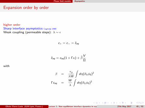
Expansion order by order
higher orderSharp interface asymptotics Caginalp 1989
Weak coupling (permeable steps): λ ∼ ε
c+ = c− = ceq
ceq = ceq(1 + Γκ) + βV
Ω
with
β =τφ
λW
∫dη(∂ηφ0)2
Γceq =W
λ
∫dη(∂ηφ0)2
Olivier Pierre-Louis (ILM-Lyon, France.) Lecture 1: Non-equilibrium interface dynamics in crystal growth 27th May 2017 45 / 92
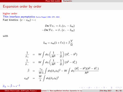
Phase field models Asympotics
Expansion order by order
higher orderThin interface asymptotics Karma Rappel 1996, OPL 2003
Fast kinetics: (c − ceq) ∼ ε
Dn.∇c+ = ν+(c+ − ceq)
−Dn.∇c− = ν−(c− − ceq)
with
ceq = ceq(1 + Γκ) + βV
Ω
1
ν+= W
∫dη
(1
M0−
1
D
)(h0− − h0)
1
ν−= W
∫dη
(1
M0−
1
D
)(h0 − h0
+)
β =τφ
Wλ
∫dη(∂ηφ0)2 −W
∫dη
(h0+ − h0)(h0 − h0
−)
M0
ceqΓ =W
λ
∫dη(∂ηφ0)2
ν± ∼ β ∼ ε−1
Olivier Pierre-Louis (ILM-Lyon, France.) Lecture 1: Non-equilibrium interface dynamics in crystal growth 27th May 2017 46 / 92
Phase field models Phase field simualtions
Contents
1 IntroductionModels and levels of descriptionAtomic steps and surface dynamics
2 Kinetic Monte CarloMaster EquationKMC algorithmKMC Simulations
3 Phase field modelsDiffuse interfaces modelsAsympoticsPhase field simualtions
4 BCF Step modelBurton-Cabrera-Frank step modelMulti-scale analysis
5 Nonlinear interface dynamicsPreamble in 0DNonlinear dynamics in 1D
6 Conclusion
Olivier Pierre-Louis (ILM-Lyon, France.) Lecture 1: Non-equilibrium interface dynamics in crystal growth 27th May 2017 47 / 92
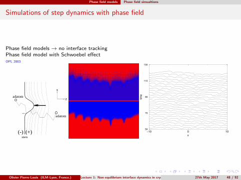
Phase field models Phase field simualtions
Simulations of step dynamics with phase field
Phase field models → no interface trackingPhase field model with Schwoebel effectOPL 2003
adatomz
x
(+)(-)step
adatom
−10 0 10
x
50
70
90
110
130
tim
e
Olivier Pierre-Louis (ILM-Lyon, France.) Lecture 1: Non-equilibrium interface dynamics in crystal growth 27th May 2017 48 / 92
Phase field models Phase field simualtions
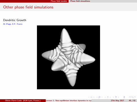
Other phase field simulations
Dendritic GrowthM. Plapp, E.P., France
Olivier Pierre-Louis (ILM-Lyon, France.) Lecture 1: Non-equilibrium interface dynamics in crystal growth 27th May 2017 49 / 92
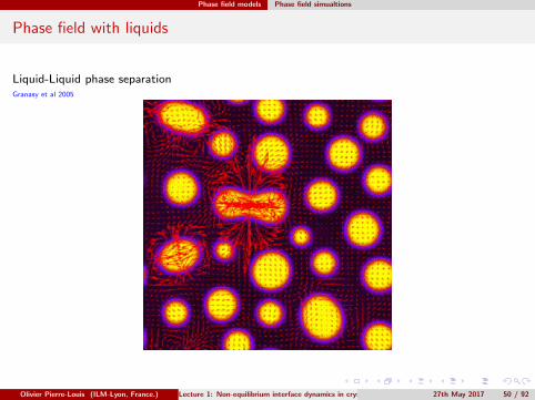
Phase field models Phase field simualtions
Phase field with liquids
Liquid-Liquid phase separationGranasy et al 2005
Olivier Pierre-Louis (ILM-Lyon, France.) Lecture 1: Non-equilibrium interface dynamics in crystal growth 27th May 2017 50 / 92
Phase field models Phase field simualtions
Conclusion
Interface tracking vs Interface Capturing → very effective numerical method
Can add, elastic strain, hydrodynamics, temperature fields, etc...
Can include fluctuations
Olivier Pierre-Louis (ILM-Lyon, France.) Lecture 1: Non-equilibrium interface dynamics in crystal growth 27th May 2017 51 / 92
BCF Step model Burton-Cabrera-Frank step model
Contents
1 IntroductionModels and levels of descriptionAtomic steps and surface dynamics
2 Kinetic Monte CarloMaster EquationKMC algorithmKMC Simulations
3 Phase field modelsDiffuse interfaces modelsAsympoticsPhase field simualtions
4 BCF Step modelBurton-Cabrera-Frank step modelMulti-scale analysis
5 Nonlinear interface dynamicsPreamble in 0DNonlinear dynamics in 1D
6 Conclusion
Olivier Pierre-Louis (ILM-Lyon, France.) Lecture 1: Non-equilibrium interface dynamics in crystal growth 27th May 2017 52 / 92
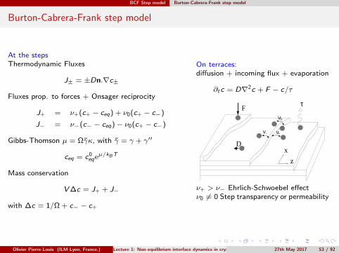
BCF Step model Burton-Cabrera-Frank step model
Burton-Cabrera-Frank step model
At the stepsThermodynamic Fluxes
J± = ±Dn.∇c±
Fluxes prop. to forces + Onsager reciprocity
J+ = ν+(c+ − ceq) + ν0(c+ − c−)
J− = ν−(c− − ceq)− ν0(c+ − c−)
Gibbs-Thomson µ = Ωγκ, with γ = γ + γ′′
ceq = c0eqeµ/kBT
Mass conservation
V∆c = J+ + J−
with ∆c = 1/Ω + c− − c+
On terraces:diffusion + incoming flux + evaporation
∂tc = D∇2c + F − c/τ
ν+ν−
ν0
τ
z
xD
F
ν+ > ν− Ehrlich-Schwoebel effectν0 6= 0 Step transparency or permeability
Olivier Pierre-Louis (ILM-Lyon, France.) Lecture 1: Non-equilibrium interface dynamics in crystal growth 27th May 2017 53 / 92
BCF Step model Burton-Cabrera-Frank step model
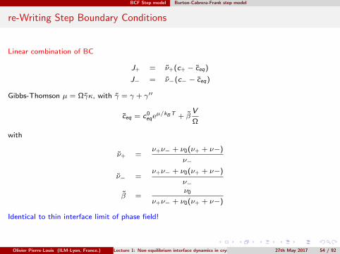
re-Writing Step Boundary Conditions
Linear combination of BC
J+ = ν+(c+ − ceq)
J− = ν−(c− − ceq)
Gibbs-Thomson µ = Ωγκ, with γ = γ + γ′′
ceq = c0eqeµ/kBT + β
V
Ω
with
ν+ =ν+ν− + ν0(ν+ + ν−)
ν−
ν− =ν+ν− + ν0(ν+ + ν−)
ν−
β =ν0
ν+ν− + ν0(ν+ + ν−)
Identical to thin interface limit of phase field!
Olivier Pierre-Louis (ILM-Lyon, France.) Lecture 1: Non-equilibrium interface dynamics in crystal growth 27th May 2017 54 / 92
BCF Step model Burton-Cabrera-Frank step model
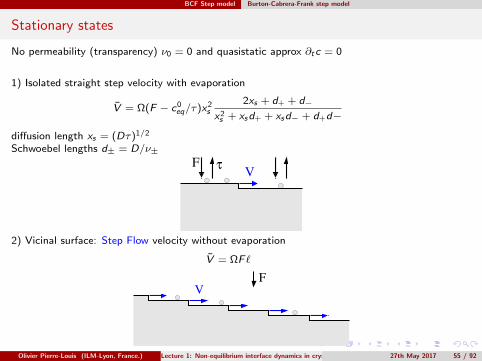
Stationary states
No permeability (transparency) ν0 = 0 and quasistatic approx ∂tc = 0
1) Isolated straight step velocity with evaporation
V = Ω(F − c0eq/τ)x2
s2xs + d+ + d−
x2s + xsd+ + xsd− + d+d−
diffusion length xs = (Dτ)1/2
Schwoebel lengths d± = D/ν±
VF τ
2) Vicinal surface: Step Flow velocity without evaporation
V = ΩF `
V
F
Olivier Pierre-Louis (ILM-Lyon, France.) Lecture 1: Non-equilibrium interface dynamics in crystal growth 27th May 2017 55 / 92
BCF Step model Multi-scale analysis
Contents
1 IntroductionModels and levels of descriptionAtomic steps and surface dynamics
2 Kinetic Monte CarloMaster EquationKMC algorithmKMC Simulations
3 Phase field modelsDiffuse interfaces modelsAsympoticsPhase field simualtions
4 BCF Step modelBurton-Cabrera-Frank step modelMulti-scale analysis
5 Nonlinear interface dynamicsPreamble in 0DNonlinear dynamics in 1D
6 Conclusion
Olivier Pierre-Louis (ILM-Lyon, France.) Lecture 1: Non-equilibrium interface dynamics in crystal growth 27th May 2017 56 / 92
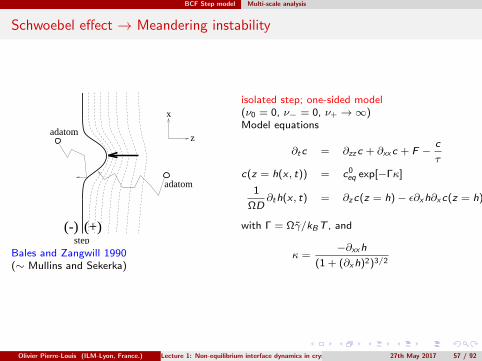
BCF Step model Multi-scale analysis
Schwoebel effect → Meandering instability
adatomz
x
(+)(-)step
adatom
Bales and Zangwill 1990(∼ Mullins and Sekerka)
isolated step; one-sided model(ν0 = 0, ν− = 0, ν+ →∞)Model equations
∂tc = ∂zzc + ∂xxc + F −c
τ
c(z = h(x , t)) = c0eq exp[−Γκ]
1
ΩD∂th(x , t) = ∂zc(z = h)− ε∂xh∂xc(z = h)
with Γ = Ωγ/kBT , and
κ =−∂xxh
(1 + (∂xh)2)3/2
Olivier Pierre-Louis (ILM-Lyon, France.) Lecture 1: Non-equilibrium interface dynamics in crystal growth 27th May 2017 57 / 92
BCF Step model Multi-scale analysis
Meandering/ Linear Analysis: Isolated step
isolated step; one-sided model (ν0 = 0, ν− = 0, ν+ →∞)
Stationary state at constant velocity
V = Ω(F − ceq/τ)(D/τ)1/2
Linear StabilitySmall perturbations, Fourier Mode
ζ(x , t) ∼ Ae iωt+iqx
Dispersion relationLong wavelength qxs 1
iω =x2s
2Ω(F − Fc )q2 −
3
4xsDΩc0
eqΓq4
→ Morphological instabilityfor F > Fc = Feq(1 + 2Γ
xs)
Bales and Zangwill 1990
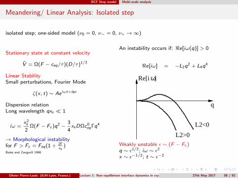
An instability occurs if: <e[iω(q)] > 0
<e[iω] = −L2q2 + L4q
4
q
Re[i ]ω
L2>0
L2<0
Weakly unstable ε ∼ (F − Fc )q ∼ ε1/2; iω ∼ ε2
x ∼ ε−1/2; t ∼ ε−2
Olivier Pierre-Louis (ILM-Lyon, France.) Lecture 1: Non-equilibrium interface dynamics in crystal growth 27th May 2017 58 / 92
BCF Step model Multi-scale analysis
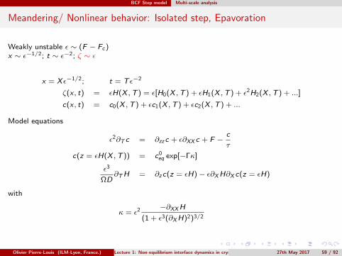
Meandering/ Nonlinear behavior: Isolated step, Epavoration
Weakly unstable ε ∼ (F − Fc )x ∼ ε−1/2; t ∼ ε−2; ζ ∼ ε
x = X ε−1/2; t = T ε−2
ζ(x , t) = εH(X ,T ) = ε[H0(X ,T ) + εH1(X ,T ) + ε2H2(X ,T ) + ...]
c(x , t) = c0(X ,T ) + εc1(X ,T ) + εc2(X ,T ) + ...
Model equations
ε2∂T c = ∂zzc + ε∂XX c + F −c
τ
c(z = εH(X ,T )) = c0eq exp[−Γκ]
ε3
ΩD∂TH = ∂zc(z = εH)− ε∂XH∂X c(z = εH)
with
κ = ε2 −∂XXH(1 + ε3(∂XH)2)3/2
Olivier Pierre-Louis (ILM-Lyon, France.) Lecture 1: Non-equilibrium interface dynamics in crystal growth 27th May 2017 59 / 92
BCF Step model Multi-scale analysis
Meandering/ Nonlinear behavior: Isolated step, Epavoration
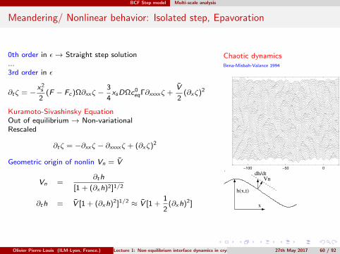
0th order in ε→ Straight step solution...3rd order in ε
∂tζ = −x2s
2(F − Fc )Ω∂xxζ −
3
4xsDΩc0
eqΓ∂xxxxζ +V
2(∂xζ)2
Kuramoto-Sivashinsky EquationOut of equilibrium → Non-variationalRescaled
∂tζ = −∂xxζ − ∂xxxxζ + (∂xζ)2
Geometric origin of nonlin Vn = V
Vn =∂th
[1 + (∂xh)2]1/2
∂th = V [1 + (∂xh)2]1/2 ≈ V [1 +1
2(∂xh)2]
Chaotic dynamicsBena-Misbah-Valance 1994
−100 −50 030
80
130
x
h(x,t)
Vndh/dt
.
Olivier Pierre-Louis (ILM-Lyon, France.) Lecture 1: Non-equilibrium interface dynamics in crystal growth 27th May 2017 60 / 92
BCF Step model Multi-scale analysis
Meandering/ Nonlinear behavior: Isolated step, Epavoration
−100 −50 030
80
130
−10 0 10
x
50
70
90
110
130
tim
e
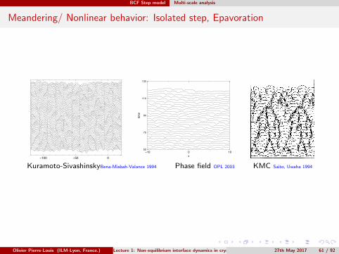
Kuramoto-SivashinskyBena-Misbah-Valance 1994 Phase field OPL 2003 KMC Saito, Uwaha 1994
Olivier Pierre-Louis (ILM-Lyon, France.) Lecture 1: Non-equilibrium interface dynamics in crystal growth 27th May 2017 61 / 92
BCF Step model Multi-scale analysis
Conclusion
Steps dynamics → nanoscale morphology
Growth, or evaporation/dissolution ...but also: electromigration, sputtering, dewetting dynamics, strain-induced instabilities, etc.
Non-equilibrium steady-states and morphological instabilities
Universality in pattern formation: Kuramoto Sivashinsky example
Olivier Pierre-Louis (ILM-Lyon, France.) Lecture 1: Non-equilibrium interface dynamics in crystal growth 27th May 2017 62 / 92
Nonlinear interface dynamics Preamble in 0D
Contents
1 IntroductionModels and levels of descriptionAtomic steps and surface dynamics
2 Kinetic Monte CarloMaster EquationKMC algorithmKMC Simulations
3 Phase field modelsDiffuse interfaces modelsAsympoticsPhase field simualtions
4 BCF Step modelBurton-Cabrera-Frank step modelMulti-scale analysis
5 Nonlinear interface dynamicsPreamble in 0DNonlinear dynamics in 1D
6 Conclusion
Olivier Pierre-Louis (ILM-Lyon, France.) Lecture 1: Non-equilibrium interface dynamics in crystal growth 27th May 2017 63 / 92
Nonlinear interface dynamics Preamble in 0D
What happens when the surface is unstable? Nonlinear Dynamics?
Preamble: simpler case with 1 degree of freedom A(t)
Olivier Pierre-Louis (ILM-Lyon, France.) Lecture 1: Non-equilibrium interface dynamics in crystal growth 27th May 2017 64 / 92
Nonlinear interface dynamics Preamble in 0D
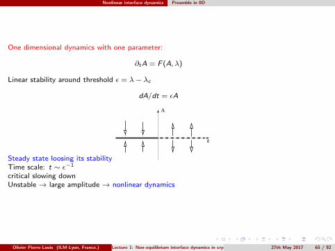
One dimensional dynamics with one parameter:
∂tA = F (A, λ)
Linear stability around threshold ε = λ− λc
dA/dt = εA
Steady state loosing its stability
A
ε
Time scale: t ∼ ε−1
critical slowing downUnstable → large amplitude → nonlinear dynamics
Olivier Pierre-Louis (ILM-Lyon, France.) Lecture 1: Non-equilibrium interface dynamics in crystal growth 27th May 2017 65 / 92
Nonlinear interface dynamics Preamble in 0D
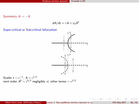
Symmetry A→ −A
dA/dt = εA + c3A3
Super-critical or Sub-critical bifurcationA
ε
A
ε
Scales t ∼ ε−1, A ∼ ε1/2
next order A5 ∼ ε5/2 negligible other terms ∼ ε3/2
Olivier Pierre-Louis (ILM-Lyon, France.) Lecture 1: Non-equilibrium interface dynamics in crystal growth 27th May 2017 66 / 92
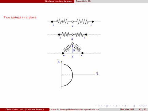
Nonlinear interface dynamics Preamble in 0D
Two springs in a plane
x
x
x
A
A
x
Olivier Pierre-Louis (ILM-Lyon, France.) Lecture 1: Non-equilibrium interface dynamics in crystal growth 27th May 2017 67 / 92
Nonlinear interface dynamics Preamble in 0D
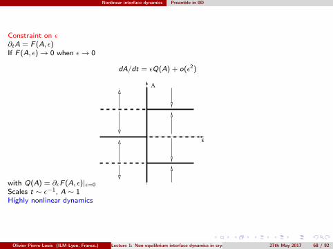
Constraint on ε∂tA = F (A, ε)If F (A, ε)→ 0 when ε→ 0
dA/dt = εQ(A) + o(ε2)
with Q(A) = ∂εF (A, ε)|ε=0
ε
A
Scales t ∼ ε−1, A ∼ 1Highly nonlinear dynamics
Olivier Pierre-Louis (ILM-Lyon, France.) Lecture 1: Non-equilibrium interface dynamics in crystal growth 27th May 2017 68 / 92

Nonlinear interface dynamics Preamble in 0D
A tube on a plane
A
θf(A)
h local heightf (A) in plane meander of the tubem particle massg gravityν frictionParticle velocity
V = −ν∂s [mgh]
∂tA = −νmg sin(θ)f ′(A)
1 + f ′(A)2
ε = sin(θ)Dynamics are highly nonlinear around θ = 0
Olivier Pierre-Louis (ILM-Lyon, France.) Lecture 1: Non-equilibrium interface dynamics in crystal growth 27th May 2017 69 / 92
Nonlinear interface dynamics Nonlinear dynamics in 1D
Contents
1 IntroductionModels and levels of descriptionAtomic steps and surface dynamics
2 Kinetic Monte CarloMaster EquationKMC algorithmKMC Simulations
3 Phase field modelsDiffuse interfaces modelsAsympoticsPhase field simualtions
4 BCF Step modelBurton-Cabrera-Frank step modelMulti-scale analysis
5 Nonlinear interface dynamicsPreamble in 0DNonlinear dynamics in 1D
6 Conclusion
Olivier Pierre-Louis (ILM-Lyon, France.) Lecture 1: Non-equilibrium interface dynamics in crystal growth 27th May 2017 70 / 92
Nonlinear interface dynamics Nonlinear dynamics in 1D
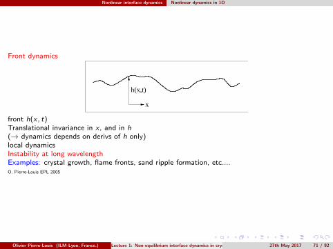
Front dynamics
x
h(x,t)
front h(x , t)Translational invariance in x , and in h(→ dynamics depends on derivs of h only)local dynamicsInstability at long wavelengthExamples: crystal growth, flame fronts, sand ripple formation, etc....O. Pierre-Louis EPL 2005
Olivier Pierre-Louis (ILM-Lyon, France.) Lecture 1: Non-equilibrium interface dynamics in crystal growth 27th May 2017 71 / 92
Nonlinear interface dynamics Nonlinear dynamics in 1D
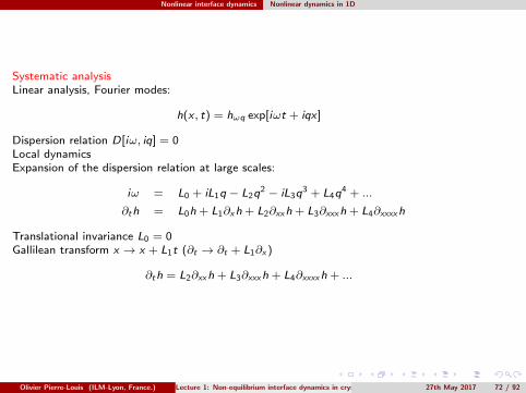
Systematic analysisLinear analysis, Fourier modes:
h(x , t) = hωq exp[iωt + iqx]
Dispersion relation D[iω, iq] = 0Local dynamicsExpansion of the dispersion relation at large scales:
iω = L0 + iL1q − L2q2 − iL3q
3 + L4q4 + ...
∂th = L0h + L1∂xh + L2∂xxh + L3∂xxxh + L4∂xxxxh
Translational invariance L0 = 0Gallilean transform x → x + L1t (∂t → ∂t + L1∂x )
∂th = L2∂xxh + L3∂xxxh + L4∂xxxxh + ...
Olivier Pierre-Louis (ILM-Lyon, France.) Lecture 1: Non-equilibrium interface dynamics in crystal growth 27th May 2017 72 / 92
Nonlinear interface dynamics Nonlinear dynamics in 1D
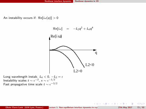
An instability occurs if: <e[iω(q)] > 0
<e[iω] = −L2q2 + L4q
4
q
Re[i ]ω
L2>0
L2<0
Long wavelength instab. L4 < 0, −L2 = εInstability scales t ∼ ε−2, x ∼ ε−1/2
Fast propagative time scale t ∼ ε−3/2
Olivier Pierre-Louis (ILM-Lyon, France.) Lecture 1: Non-equilibrium interface dynamics in crystal growth 27th May 2017 73 / 92
Nonlinear interface dynamics Nonlinear dynamics in 1D
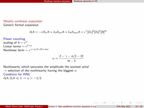
Weakly nonlinear expansionGeneric formal expansion
∂th = −ε∂xxh + L3∂xxxh + L4∂xxxxh + εγ [∂x ]n[∂t ]`[h]m
Power countingscaling of h ∼ εαLinear terms ∼ ε2+α
Nonlinear term ∼ εγ+n/2+2`+mα
α =2− γ − n/2− 2`
m − 1
Nonlinearity which saturates the amplitude the soonest wins!→ selection of the nonlinearity having the biggest αCondition for WNL∂th, ∂xh 1→ α > −1/2
Olivier Pierre-Louis (ILM-Lyon, France.) Lecture 1: Non-equilibrium interface dynamics in crystal growth 27th May 2017 74 / 92
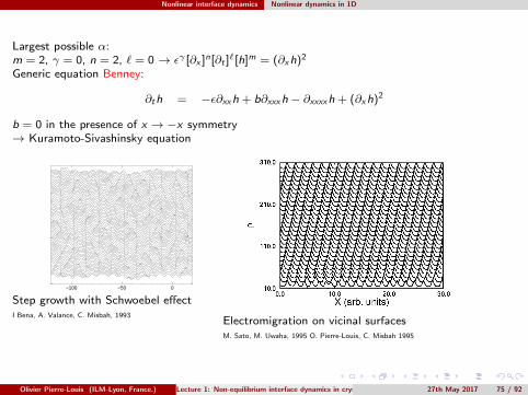
Nonlinear interface dynamics Nonlinear dynamics in 1D
Largest possible α:m = 2, γ = 0, n = 2, ` = 0 → εγ [∂x ]n[∂t ]`[h]m = (∂xh)2
Generic equation Benney:
∂th = −ε∂xxh + b∂xxxh − ∂xxxxh + (∂xh)2
b = 0 in the presence of x → −x symmetry→ Kuramoto-Sivashinsky equation
−100 −50 030
80
130
Step growth with Schwoebel effectI Bena, A. Valance, C. Misbah, 1993
Electromigration on vicinal surfacesM. Sato, M. Uwaha, 1995 O. Pierre-Louis, C. Misbah 1995
Olivier Pierre-Louis (ILM-Lyon, France.) Lecture 1: Non-equilibrium interface dynamics in crystal growth 27th May 2017 75 / 92
Nonlinear interface dynamics Nonlinear dynamics in 1D
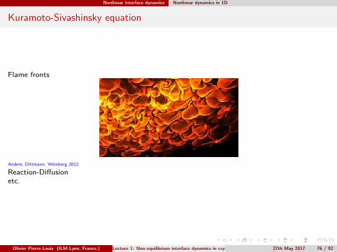
Kuramoto-Sivashinsky equation
Flame fronts
Anders, Dittmann, Weinberg 2012
Reaction-Diffusionetc.
Olivier Pierre-Louis (ILM-Lyon, France.) Lecture 1: Non-equilibrium interface dynamics in crystal growth 27th May 2017 76 / 92

Nonlinear interface dynamics Nonlinear dynamics in 1D
Conservation law
∂th = −∂x j
x
h(x,t)
j
Vicinity to thermodynamic equilibrium(or variational steady-state)driving force ε
∂th = ∂x
[M∂x
δFδh− εJ
]+ o(ε2)
Highly nonlinear dynamics h ∼ ε−1/2
∂th = ∂x [εA + B∂xxC ]
where A,B,C functions of ∂xh ∼ 1x → −x symmetry; non-variational→ Examples in Molecular Beam Epitaxy
Olivier Pierre-Louis (ILM-Lyon, France.) Lecture 1: Non-equilibrium interface dynamics in crystal growth 27th May 2017 77 / 92
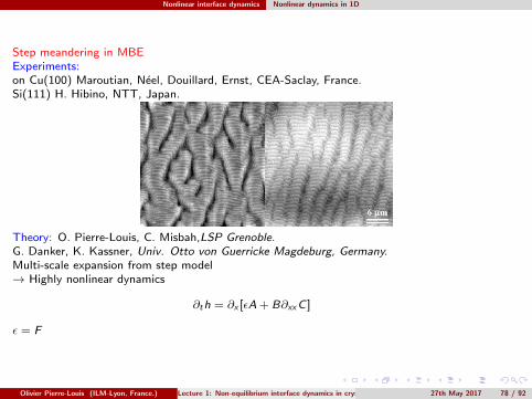
Nonlinear interface dynamics Nonlinear dynamics in 1D
Step meandering in MBEExperiments:on Cu(100) Maroutian, Neel, Douillard, Ernst, CEA-Saclay, France.Si(111) H. Hibino, NTT, Japan.
Theory: O. Pierre-Louis, C. Misbah,LSP Grenoble.G. Danker, K. Kassner, Univ. Otto von Guerricke Magdeburg, Germany.Multi-scale expansion from step model→ Highly nonlinear dynamics
∂th = ∂x [εA + B∂xxC ]
ε = F
Olivier Pierre-Louis (ILM-Lyon, France.) Lecture 1: Non-equilibrium interface dynamics in crystal growth 27th May 2017 78 / 92
Nonlinear interface dynamics Nonlinear dynamics in 1D
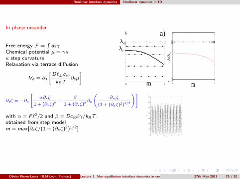
In phase meander
Free energy F =∫dsγ
Chemical potential µ = γκκ step curvatureRelaxation via terrace diffusion
Vn = ∂s
[D`⊥ceq
kBT∂sµ
]
∂tζ = −∂x
[α∂xζ
1 + (∂xζ)2+
β
1 + (∂xζ)2∂x
(∂xxζ
(1 + (∂xζ)2)3/2
)]
with α = F `2/2 and β = Dceq`γ/kBT .obtained from step modelm = max[∂xζ/(1 + (∂xζ)2)1/2]
0 1m 0
1
λ/λ
m
λc
λm
λ
0 1m
a)
0 20 40 60 80x
0
200
400
600
800
1000
1200
1400
t
Olivier Pierre-Louis (ILM-Lyon, France.) Lecture 1: Non-equilibrium interface dynamics in crystal growth 27th May 2017 79 / 92
Nonlinear interface dynamics Nonlinear dynamics in 1D
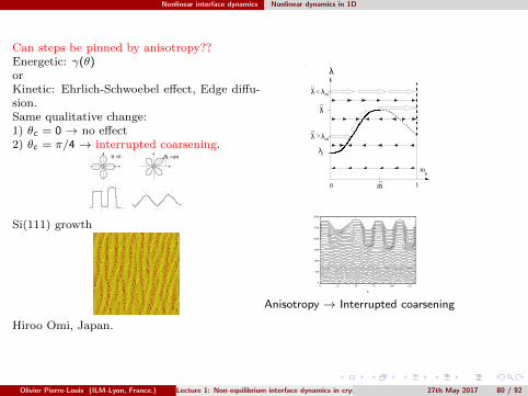
Can steps be pinned by anisotropy??Energetic: γ(θ)orKinetic: Ehrlich-Schwoebel effect, Edge diffu-sion.Same qualitative change:1) θc = 0 → no effect2) θc = π/4 → interrupted coarsening.
θ =0 θ =π/4c c
Si(111) growth
Hiroo Omi, Japan.
λc
λ∼
λm<
λmλ∼
>
λ∼
∼m
m0
λ
0 1
0 25 50 75 100 125
x
0
500
1000
1500
2000
2500
3000
Anisotropy → Interrupted coarsening
Olivier Pierre-Louis (ILM-Lyon, France.) Lecture 1: Non-equilibrium interface dynamics in crystal growth 27th May 2017 80 / 92

Nonlinear interface dynamics Nonlinear dynamics in 1D
Elastic interactions in homo-epitaxy:
σ
f
fσ
Force dipoles at step:→ interaction energy ∼ 1/`2
between straight steps.
λc
∼m
m0
λm
λ
0 1
0 20 40 60 80x
0
200
400
600
800
1000
1200
1400
Elastic interactions → endless coarsening
Olivier Pierre-Louis (ILM-Lyon, France.) Lecture 1: Non-equilibrium interface dynamics in crystal growth 27th May 2017 81 / 92
Nonlinear interface dynamics Nonlinear dynamics in 1D
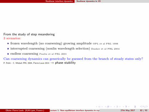
From the study of step meandering3 scenarios:
frozen wavelength (no coarsening) growing amplitude OPL et al PRL 1998
interrupted coarsening (nonlin wavelength selection) Danker et al PRL 2004
endless coarsening Paulin et al PRL 2001
Can coarsening dynamics can generically be guessed from the branch of steady states only?P. Politi - C. Misbah PRL 2004, Pierre-Louis 2014 → phase stability
Olivier Pierre-Louis (ILM-Lyon, France.) Lecture 1: Non-equilibrium interface dynamics in crystal growth 27th May 2017 82 / 92
Nonlinear interface dynamics Nonlinear dynamics in 1D
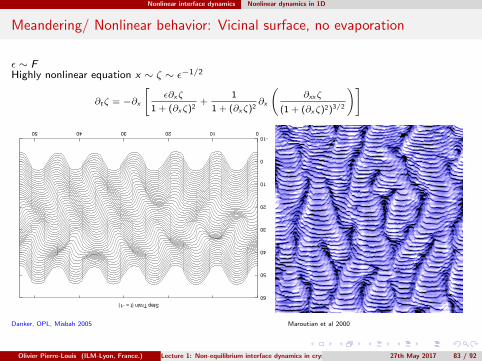
Meandering/ Nonlinear behavior: Vicinal surface, no evaporation
ε ∼ FHighly nonlinear equation x ∼ ζ ∼ ε−1/2
∂tζ = −∂x
[ε∂xζ
1 + (∂xζ)2+
1
1 + (∂xζ)2∂x
(∂xxζ
(1 + (∂xζ)2)3/2
)]
-10
0
10
20
30
40
50
60
01020304050
Step Train (t = -1)
Danker, OPL, Misbah 2005 Maroutian et al 2000
Olivier Pierre-Louis (ILM-Lyon, France.) Lecture 1: Non-equilibrium interface dynamics in crystal growth 27th May 2017 83 / 92
Nonlinear interface dynamics Nonlinear dynamics in 1D
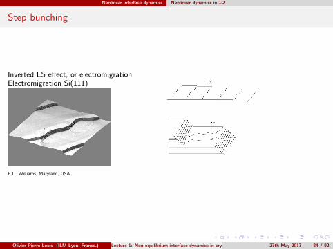
Step bunching
Inverted ES effect, or electromigrationElectromigration Si(111)
E.D. Williams, Maryland, USA
Olivier Pierre-Louis (ILM-Lyon, France.) Lecture 1: Non-equilibrium interface dynamics in crystal growth 27th May 2017 84 / 92
Nonlinear interface dynamics Nonlinear dynamics in 1D
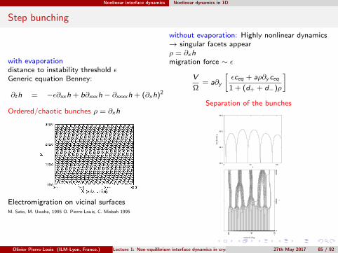
Step bunching
with evaporationdistance to instability threshold εGeneric equation Benney:
∂th = −ε∂xxh + b∂xxxh − ∂xxxxh + (∂xh)2
Ordered/chaotic bunches ρ = ∂xh
Electromigration on vicinal surfacesM. Sato, M. Uwaha, 1995 O. Pierre-Louis, C. Misbah 1995
without evaporation: Highly nonlinear dynamics→ singular facets appearρ = ∂xhmigration force ∼ ε
V
Ω= a∂y
[εceq + aρ∂y ceq
1 + (d+ + d−)ρ
]Separation of the bunches
0 50 100
y
9810
9811
9812
9813
ste
p d
ensity
ρ
010000
20000
t
−20
80
180
Step position
Olivier Pierre-Louis (ILM-Lyon, France.) Lecture 1: Non-equilibrium interface dynamics in crystal growth 27th May 2017 85 / 92
Nonlinear interface dynamics Nonlinear dynamics in 1D
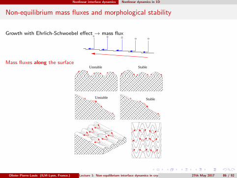
Non-equilibrium mass fluxes and morphological stability
Growth with Ehrlich-Schwoebel effect → mass flux
Mass fluxes along the surface
Unstable
Unstable
Stable
Stable
Olivier Pierre-Louis (ILM-Lyon, France.) Lecture 1: Non-equilibrium interface dynamics in crystal growth 27th May 2017 86 / 92
Nonlinear interface dynamics Nonlinear dynamics in 1D
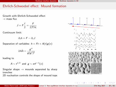
Ehrlich-Schwoebel effect: Mound formation
Growth with Ehrlich-Schwoebel effect→ mass flux
J = F`
2=
F
2|∇h|
Continuum limit:
∂th = F − ∂xJ
Separation of varliables: h = Ft + A(t)g(x)
2AA =g ′′
g(g ′)2
leading to
A ∼ t1/2 and g ∼ erf −1(x)
Singular shape → mounds separated by sharptrenches2D nucleation controls the shape of mound tops
Olivier Pierre-Louis (ILM-Lyon, France.) Lecture 1: Non-equilibrium interface dynamics in crystal growth 27th May 2017 87 / 92
Nonlinear interface dynamics Nonlinear dynamics in 1D
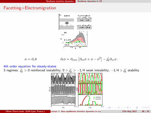
Facetting+Electromigration
φ = ∂xh ∂tφ = ∂xxxx[∂xxφ+ φ− φ3
]− j ′E∂xxφ .
4th order equation for steady-states3 regimes: j ′E > 0 reinforced instability; 0 > j ′E > −1/4 weak instability; −1/4 > j ′E stability
time
0 0.2x/L0 0.2x/L
h(x,
t)
j’E > 0
-1/4 < j’E < 0
j’E < -1/4
minimamaxima
(a)
(b)
(c)
Olivier Pierre-Louis (ILM-Lyon, France.) Lecture 1: Non-equilibrium interface dynamics in crystal growth 27th May 2017 88 / 92
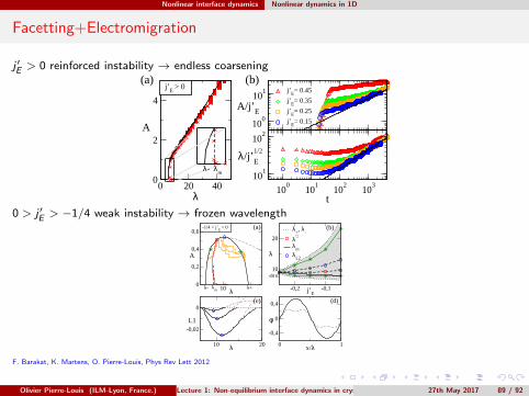
Nonlinear interface dynamics Nonlinear dynamics in 1D
Facetting+Electromigration
j ′E > 0 reinforced instability → endless coarsening
100
101
A/j’E
j’E= 0.45
j’E= 0.35
j’E= 0.25
j’E= 0.15
100
101
102
103
t
101
102
λ/j’E
0 20 40λ
0
2
4
A
j’E
> 0
1/2
(a) (b)
λm
λ-
0 > j ′E > −1/4 weak instability → frozen wavelength
-0,2 -0,1j’E
10
20
λ
λ+, λ
-
λ∗
λm
λL2
10 λ0
0,2
0,4
0,6
A
10 20λ
-0,02
0
L1
0 1x/λ
-0,4
0
0,4
φ
-1/4 < j’E
< 0
√8 π
(a)
(c) (d)
(b)
λ- λ+λm
F. Barakat, K. Martens, O. Pierre-Louis, Phys Rev Lett 2012
Olivier Pierre-Louis (ILM-Lyon, France.) Lecture 1: Non-equilibrium interface dynamics in crystal growth 27th May 2017 89 / 92
Nonlinear interface dynamics Nonlinear dynamics in 1D
Conclusion
weakly vs highly nonlinear dynamics
Fronts close to thermodyn equil, or variational steady-state (Lyapunov functional)
Higher order problems?
Other examples of Highly nonlinear dynamics
Step bunchingJ. Chang, O. Pierre-Louis, C. Misbah, PRL 2006
Oscillatory driving of crystal surfacesO Pierre-Louis, M.I. Haftel, PRL 2001
Similar results without translational invarianceO. Pierre-Louis EPL 2005
Olivier Pierre-Louis (ILM-Lyon, France.) Lecture 1: Non-equilibrium interface dynamics in crystal growth 27th May 2017 90 / 92
Conclusion
Conclusion
Modelling Crystal Surface Dynamics
Tools
KMC
Phase field
Sharp interface models (such as BCF Step models)
Phenomena
Growth-dissolution rate
Kinetic Roughening
Morphology: relaxation or instabilities → patterns
Global remarks
Surface Diffusion vs Bulk diffusion
Faithful microscopic vs Effective dynamics
Multi-scale modeling
Olivier Pierre-Louis (ILM-Lyon, France.) Lecture 1: Non-equilibrium interface dynamics in crystal growth 27th May 2017 91 / 92

Conclusion
Conclusion
ReferencesBooks
A.L. Barabasi, H.E. Stanley, Fractal Concepts in Surface growth, Cambridge, (1995)
Y. Saito, Statistical Physics of Crystal Growth, Worl Scientific (1996)
A. Pimpinelli and J. Villain, Physics of crystal growth, Cambridge, (1998)
J. Krug, and T. Michely, Islands, Mounds, and Atoms, Springer (2004)
C. Misbah, Complex Dynamics and Morphogenesis: An Introduction to Nonlinear Science(2017)
Reviews
Burton Carbrera Frank, The Growth of Crystals and the Equilibrium Structure of theirSurfaces, Phil. Trans. A, (1951)
M. Kotrla, Computer Physics Communications 97 82-100 (1996)
C. Misbah, O. Pierre-Louis, Y. Saito, Rev Mod Phys 82 981 (2010).
Olivier Pierre-Louis (ILM-Lyon, France.) Lecture 1: Non-equilibrium interface dynamics in crystal growth 27th May 2017 92 / 92