oil price dynamics (2002 2006) - institut für …bwl.univie.ac.at/.../oilpricedynamics.pdf · ·...

Available online at www.sciencedirect.com

er.com/locate/eneco
Energy Economics 30 (2008) 2134–2153
www.elsevi

Oil price dynamics (2002–2006)☆

Hossein Askari a,⁎, Noureddine Krichene b

a George Washington University, United Statesb International Monetary Fund, United States

Received 5 September 2007; received in revised form 4 December 2007; accepted 27 December 2007Available online 9 January 2008

Abstract

Oil price dynamics during 2002–2006 have been characterized by high volatility, high intensity jumps,and strong upward drift, and were concomitant with underlying fundamentals of oil markets and worldeconomy; namely, pressure on oil prices resulting from rigid crude oil supply and expanding world demandfor crude oil. A change in the oil price process parameters would require a change in underlyingfundamentals. Market expectations, extracted from call and put option prices, anticipated no change inunderlying fundamentals in the short term. Markets expected oil prices to remain volatile and jumpy, andwith higher probabilities, to rise, rather than fall, above the expected mean.© 2008 Elsevier B.V. All rights reserved.

JEL classification: C10; C20; C32; Q4

Keywords: Characteristic function; Crude oil; Cumulants; Drift; Jump–diffusion; Kurtosis; Option pricing; Skewness;Variance-gamma distribution; Volatility

☆ The authors are grateful for very helpful comments and suggestions from an anonymous referee.⁎ Corresponding author.E-mail addresses: [email protected] (H. Askari), [email protected] (N. Krichene).

0140-9883/$ - see front matter © 2008 Elsevier B.V. All rights reserved.doi:10.1016/j.eneco.2007.12.004

mailto:[email protected]

mailto:[email protected]

http://dx.doi.org/10.1016/j.eneco.2007.12.004

2135H. Askari, N. Krichene / Energy Economics 30 (2008) 2134–2153

1. Introduction

Knowledge of stochastic process underlying crude oil prices is important not only for pricingderivatives and hedging, but also for policymaking and short-term forecasting.1

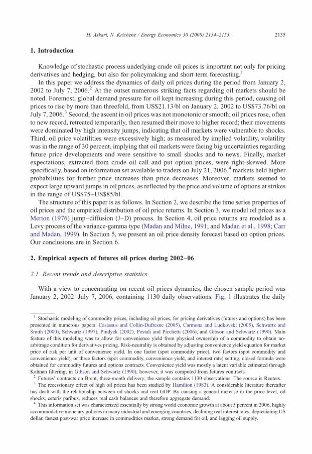
In this paper we address the dynamics of daily oil prices during the period from January 2,2002 to July 7, 2006.2 At the outset numerous striking facts regarding oil markets should benoted. Foremost, global demand pressure for oil kept increasing during this period, causing oilprices to rise by more than threefold, from US$21.13/bl on January 2, 2002 to US$73.76/bl onJuly 7, 2006.3 Second, the ascent in oil prices was not monotonic or smooth; oil prices rose, oftento new record, retreated temporarily, then resumed their move to higher record; their movementswere dominated by high intensity jumps, indicating that oil markets were vulnerable to shocks.Third, oil price volatilities were excessively high; as measured by implied volatility, volatilitywas in the range of 30 percent, implying that oil markets were facing big uncertainties regardingfuture price developments and were sensitive to small shocks and to news. Finally, marketexpectations, extracted from crude oil call and put option prices, were right-skewed. Morespecifically, based on information set available to traders on July 21, 2006,4 markets held higherprobabilities for further price increases than price decreases. Moreover, markets seemed toexpect large upward jumps in oil prices, as reflected by the price and volume of options at strikesin the range of US$75–US$85/bl.

The structure of this paper is as follows. In Section 2, we describe the time series properties ofoil prices and the empirical distribution of oil price returns. In Section 3, we model oil prices as aMerton (1976) jump–diffusion (J–D) process. In Section 4, oil price returns are modeled as aLevy process of the variance-gamma type (Madan and Milne, 1991; and Madan et al., 1998; Carrand Madan, 1999). In Section 5, we present an oil price density forecast based on option prices.Our conclusions are in Section 6.

2. Empirical aspects of futures oil prices during 2002–06

2.1. Recent trends and descriptive statistics

With a view to concentrating on recent oil prices dynamics, the chosen sample period wasJanuary 2, 2002–July 7, 2006, containing 1130 daily observations. Fig. 1 illustrates the daily

1 Stochastic modeling of commodity prices, including oil prices, for pricing derivatives (futures and options) has beenpresented in numerous papers: Casassus and Collin-Dufresne (2005), Carmona and Ludkovski (2005), Schwartz andSmith (2000), Schwartz (1997), Pindyck (2002), Postali and Picchetti (2006), and Gibson and Schwartz (1990). Mainfeature of this modeling was to allow for convenience yield from physical ownership of a commodity to obtain no-arbitrage condition for derivatives pricing. Risk-neutrality is obtained by adjusting convenience yield equation for marketprice of risk per unit of convenience yield. In one factor (spot commodity price), two factors (spot commodity andconvenience yield), or three factors (spot commodity, convenience yield, and interest rate) setting, closed formula wereobtained for commodity futures and options contracts. Convenience yield was mostly a latent variable estimated throughKalman filtering; in Gibson and Schwartz (1990), however, it was computed from futures contracts.2 Futures' contracts on Brent, three-month delivery; the sample contains 1130 observations. The source is Reuters.3 The recessionary effect of high oil prices has been studied by Hamilton (1983). A considerable literature thereafter

has dealt with the relationship between oil shocks and real GDP. By causing a general increase in the price level, oilshocks, ceteris paribus, reduces real cash balances and therefore aggregate demand.4 This information set was characterized essentially by strong world economic growth at about 5 percent in 2006, highly

accommodative monetary policies in many industrial and emerging countries, declining real interest rates, depreciating USdollar, fastest post-war price increase in commodities market, strong demand for oil, and lagging oil supply.

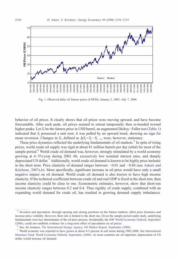
Fig. 1. Observed daily oil futures prices (US$/bl), January 2, 2002–July 7, 2006.

2136 H. Askari, N. Krichene / Energy Economics 30 (2008) 2134–2153

behavior of oil prices. It clearly shows that oil prices were moving upward, and have becomeforecastable. After each peak, oil prices seemed to retreat temporarily then re-trended towardhigher peaks. Let St be the futures price in US$/barrel, an augmented Dickey–Fuller test (Table 1)indicated that St possessed a unit root; it was pulled by an upward trend, showing no sign formean reversion. Changes in St, defined as ΔSt=St−St− 1, were, however, stationary.

These price dynamics reflected the underlying fundamentals of oil markets.5 In spite of risingprices, world crude oil supply was rigid at about 81 million barrels per day (mbd) for most of thesample period.6 World crude oil demand was, however, strongly stimulated by a world economygrowing at 4–5%/year during 2002–06, excessively low nominal interest rates, and sharplydepreciated US dollar.7 Additionally, world crude oil demand is known to be highly price inelasticin the short term. Price elasticity of demand ranges between −0.01 and −0.04 (see Askari andKrichene, 2007a,b). More specifically, significant increase in oil price would have only a smallnegative impact on oil demand. World crude oil demand is also known to have high incomeelasticity. If the technical coefficient between crude oil and real GDP is fixed in the short tem, thenincome elasticity could be close to one. Econometric estimates, however, show that short-runincome elasticity ranges between 0.2 and 0.4. Thus rigidity of crude supply, combined with anexpanding world demand for crude oil, has resulted in growing demand–supply imbalances.

5 Investors and speculators, through opening and closing positions on the futures markets, affect price dynamics andincrease price volatility. However, their role is limited to the short run. Given the sample period under study, underlyingfundamentals were key determinants of the oil price process. Incidentally, the IMF World Economic Outlook, September(2006), could not establish evidence for a long-term effect of speculation on oil prices.6 See, for instance, The International Energy Agency, Oil Market Report, September (2006).7 World economy was reported to have grown at about 4-5 percent in real terms during 2002-2006. See International

Monetary Fund, World Economic Outlook, September, (2006). As most countries are oil importers, depreciation of USdollar would increase oil demand.

Table 1Time-series properties of oil prices

Augmented Dickey–Fuller unit-root test on oil price.Null hypothesis: St has a unit root.Augmented Dickey–Fuller test statistic=−0.52; probability value=0.88.Test critical values: 1% level (−3.44); 5% level (−2.86); 10% level (−2.57).Null hypothesis: ΔSt=St−St−1 has a unit root.Augmented Dickey–Fuller test statistic=−35.98; probability value=0.00.Test critical values: 1% level (−3.44); 5% level (−2.86); 10% level (−2.57).


Given price inelasticities of both oil demand and supply, even a small excess demand (supply) foroil would require large changes in oil prices to clear markets.

Additional insight into oil price dynamics is gained by analyzing log-price return defined asxt=ΔlogSt=logSt− logSt− 1. The graph for these changes (Fig. 2) shows that large jumps in crudeoil prices were frequent and had a relatively high probability. Although the mode was around 1–2

Fig. 2. Daily crude oil price returns distribution, January 2, 02–July 7, 06. Descriptive statistics: mean=0.116; standarddeviation=2.29; skewness=−0.39; kurtosis=4.79; Jarque–Bera normality statistics=179.3, probability-value=0.0.

Fig. 3. Extimated GARCH (1,1) Volatility, January 2–July 06.


percent, daily changes in the range of 5–7% were not uncommon.8 The empirical distribution hada large dispersion, with standard deviation estimated at 2.29 (annualized to 36.3 percent). Thedistribution was left-skewed, implying that downward jumps of smaller size were more frequentthan upward jumps of larger size; as the mean was positive and high, smaller jumps wereoutweighed by larger jumps. The distribution had also fat tails, meaning that large jumps tendedto occur more frequently than in the normal case. These empirical findings on daily oil futuresprices were typical of financial time series as noted in Clark (1973), Fama (1965), and Mandelbrot(1963). These facts suggested modeling the oil price process as a jump-diffusion or, in a moregeneral way, as a Levy process (Cont and Tankov, 2004a).

2.2. Oil price time-varying volatility

Volatility measures uncertainty and also sensitivity of prices to news and shocks, and is a keyparameter in option pricing. Volatility was also computed using a GARCH model for data ondaily oil futures prices covering January 2, 2002–July 7, 2006 (Fig. 3). The oil price return wasdefined as: xt=ΔlogSt=logSt− logSt− 1.

9 The fitting of the GARCH model showed high pricevolatility, periods of volatility clustering, followed by some reversion to a mean volatilityestimated at 43 percent. GARCH volatility was rising during periods of large price shocks,stimulating speculation and leading to volatility clustering; it was, however, receding duringperiods of price retreat. It implied that oil markets were constantly experiencing large un-certainties and were affected by frequent shocks.

3. Crude oil price as a Merton jump–diffusion process

3.1. The stochastic differential equation for the jump–diffusion model

Based on the empirical findings discussed in the previous section, namely the presence ofskewness and kurtosis in the empirical distribution of oil price returns, an adequate model for oilprices would be a jump–diffusion model. In fact, Merton (1976), recognizing the presence of jumpsin asset prices and for more accurate option pricing, proposed modeling these prices as a jump–diffusion process instead of a pure diffusion model. Moreover, it is well-known that short-termoptions have market implied volatilities that exhibit a significant skew across strikes.10 In thisconnection, Bakshi et al. (1997) argued that pure diffusion based models could not adequatelyexplain the smile effect in short-dated option prices and emphasized the importance of adding a jumpcomponent in modeling asset price dynamics. In the same vein, Bates (1996) noted that diffusion-based stochastic volatility models could not explain skewness in implied volatilities, except underimplausible values for the model's parameters. Models with jumps generically lead to significantskews for short-term maturities. More generally, adding jumps to returns in a diffusion-basedstochastic volatility model, the resulting model can generate sufficient variability and asymmetry inthe short-term returns to match implied volatility skews for short-term maturities.

8 The frequency of jumps exceeding ±3 percent was estimated from the sample at 23 percent.9 GARCH stands for Generalized Autoregressive Conditional Heteroskedasticity. A GARCH (1,1) model is defined as

follows: The mean equation: xt=ΔlogSt=c+εt, εt~N(0,σt2) The conditional variance equation: σt

2=ω+αεt - 12 +βσt-1

2 ,where σt

2=E(εt2).

10 Implied volatility is the volatility which equates the Black and Scholes (1973) call option pricing formula with the calloption's market value.


Accordingly, the continuous-time stochastic process driving crude oil prices can be stated as aJ–D process given by a stochastic differential equation (SDE):

dStSt

¼ αdt þ σdBt þ exp Jtð Þ � 1ð ÞdNt ð1Þ

St denotes crude oil price, α is the instantaneous return, and σ2 is the instantaneous variance.The continuous component is given by a standard Brownian motion, Bt, distributed as dBt~N(0,dt). The discontinuities of the price process are described by a Poisson counterNt, characterized byits intensity, λ, and jump size, Jt. The Brownian motion and the Poisson process are independent.The intensity of the Poisson process describes the mean number of arrivals of abnormalinformation per unit of time and is expressed as: Prob[ΔNt=1]=λdt, and Prob[ΔNt=0]=1−λdt.When abnormal information arrives, crude oil price jumps from St− (limit from left) to St=exp(Jt)St−. The percentage change is measured by (exp(Jt)−1). The jump size, Jt, is independent ofBt and Nt, and is assumed to be normally distributed: Jt~N(β,δ

2). Letting Xt=log(St) and using Ito'slemma, the log-price return process becomes:

dXt ¼ α� 12σ2

� �dt þ σdBt þ JtdNt ¼ Adt þ σdBt þ JtdNt ð2Þ

where A ¼ α� 12σ

2� �

.11 The parameter vector associated with the price process is therefore θ=(μ,σ2, λ, β, δ2). Discretized over (t, t+Δ), the model takes the form:

DXt ¼ ADþ σDBt þXDNt

i¼0

Ji ð3Þ

Where ΔBt=Bt+Δ−Bt~N(0, Δ), and ΔNt=Nt+Δ−Nt is the actual number of jumps occurringduring the time interval (t, t+Δ), and Ji are independently and identically distributed as Ji~N(β,δ2). The log-return, xt=ΔXt, therefore includes the sum of two independent components: adiffusion component with drift and a jump component. Its probability density is a convolution oftwo independent random variables and can be expressed as:12

f xð Þ ¼Xln¼0

kDð Þne�kD

n!1ffiffiffiffiffiffiffiffiffiffiffiffiffiffiffiffiffiffiffiffiffiffiffiffiffiffiffiffiffiffiffi

2p σ2Dþ nd2� �q exp � x� AD� nbð Þ2

2 σ2Dþ nd2� �

!264

375 ð4Þ

With n=0,1,2,........ Putting Δ=1, i.e., the time interval is (t, t+1), the density functionbecomes

f xð Þ ¼Xln¼0

kð Þne�k

n!1ffiffiffiffiffiffiffiffiffiffiffiffiffiffiffiffiffiffiffiffiffiffiffiffiffiffiffi

2p σ2 þ nd2� �q exp � x� A� nbð Þ2

2 σ2 þ nd2� �

!264

375 ð5Þ

11 A solution to this SDE can be written as ST ¼ S 0ð Þexp α� 12σ

2� �

T þ σBT þPNTi¼0 Ji

h i.

12 Ball and Torous (1983) modeled the jump component inMerton's model as a Bernoulli process. In this respect, either one orno abnormal event occurs during the time interval (t, t+Δ), with Prob[one abnormal event] =λΔ, Prob[no abnormalevent]=1−λΔ, and Prob[more than one abnormal event]=0. The density function for the log-return becomes: f (x) =N(μΔ+β, σ2Δ+ δ2)(λΔ) +N(μΔ, σ2Δ)(1−λΔ).


3.2. Alternative methods for estimating the jump–diffusion model: maximum likelihood, methodof cumulants, and method of characteristic function

3.2.1. The maximum likelihood methodLet x={x1, x2,.......,xT} be an observed sample of log-returns, the log-likelihood function can

be expressed as:

L h; xð Þ ¼ �Tk� T2ln 2pð Þ þ

XTt¼1

lnXln¼0

kn

n!1ffiffiffiffiffiffiffiffiffiffiffiffiffiffiffiffiffiffi

σ2 þ nd2p exp

� xt � A� nbð Þ22 σ2 þ nd2� �

!" #ð6Þ

Application of the maximum likelihood (ML) method for estimating the J–D model has metwith difficulties arising mainly from identification of jump parameter and instability of parameterestimates. Nonetheless, Ball and Torous (1985) applied directly the ML method by truncating thenumber of jumps at n=10. Ball and Torous (1985) and Jorion (1988) applied the ML method byassuming a Bernoulli process for the jump component. While the ML estimates achieve thelower bound for Cramer–Rao efficiency criterion, difficulties with the likelihood function arisingfrom computational tractability, un-boundedness over the parameter space, and instability ofparameters, have led researchers to explore alternative estimation methods, based essentially onthe method of moments.

3.2.2. The method of cumulants(See Annex): Press (1967) used the method of cumulants as described in Kendall and Stuart

(1977) to estimate the J–D model. Define the characteristic function (CF) of Xt as:

/X uð Þ ¼ E exp iuXtð Þ½ � ¼R

exp iuXtð Þf Xtð ÞdXt ð7Þ

where f(Xt) is the probability density function of Xt, u is the transform variable, andffiffiffiffiffiffiffi�1

p ¼ i.13

The cumulants of Xt, denoted by jn, n=0, 1, 2,…, are the coefficients in the power seriesexpansion of the logarithm of the CF of Xt, expressed as:

ln/ uð Þ ¼Xln¼1

jniuð Þnn!

¼ 1þ j1iuð Þ1!

þ j2iuð Þ22!

þ N þ jniuð Þnn!

þ N ð8Þ

Noting that the CF for the jump-diffusion process is given by:14,15

/X1uð Þ ¼ exp �σ2u2

2þ iAuþ k exp ibu� d2u2

2

� �� 1

� �� ð9Þ

13 The characteristic function ϕX (u) is related to the moment generating function (MGF) GX (u) GX uð Þ ¼ E exp uXtð Þ½ � ¼Rexp uXtð ÞdF Xtð Þ by a change of the transform variable u→− iu, namely GX (iu)=ϕX (u), and GX (u)=ϕX (− iu).14 See, for instance, Madan and Seneta (1987), and Cont and Tankov (2004a,b).15 Moment generating function for J–D process is: MGF uð Þ ¼ E euXtð Þ ¼ exp σ2u2

2 þ Auþ k exp buþ d2u22

� 1

h i. If the J–D

is modeled as Bernoulli mixture of normal densities, i.e., log-return are given by: f(x)=N(μ+β, σ2+δ2)(λ)+N(μ, σ2)(1−λ),then MGF function is given by: MGF uð Þ ¼ kexp

σ2þd2ð Þu22 þ Aþ bð Þu

� �þ 1� kð Þexp σ2u2

2 þ Auh i

.


It follows that the first four cumulants of the J–D process are:

j1 ¼ Aþ kb; j2 ¼ σ2 þ kd2 þ kb2; j3 ¼ kb 3d2 þ b2� �

;

j4 ¼ k 3d4 þ 6b2d2 þ b4� � ð10Þ

Obviously, the cumulants enable to recover J–D parameters from sample moments. Press(1967), in order to avoid using higher order cumulants, imposed the restriction μ=0 and derivedthe following relations:

b4 �2

j3j1

b2 þ 3j4

2j1b� j23

2j21¼ 0; k ¼ j1

b; d

2 ¼ j3 � b2j1

3j1;

σ2 ¼ j2 � j1b

b2 þ j3 � b

2j1

3j1

!:

ð11Þ

Press' estimates often carried wrong-sign and were not plausible. Beckers (1981) adopted thesame method as Press, however, setting β, instead of μ, to zero. Using sixth order cumulants, hiscumulant equations yielded the following system:

A¼ j1; k ¼ 25j343j26

; d2 ¼ j6

5j4; σ2 ¼ j2 � 5j24

3j6ð12Þ

Beckers' estimates improved those of Press, yet they were not free of anomalies. Ball andTorous (1983), using a Bernoulli, instead of a Poisson, jump process and maintaining Beckers'restriction, i.e. β=0, derived the following cumulant equations:

j1 ¼ A;j2 ¼ σ2 þ kd2; j3 ¼ 0; j4 ¼ 3d2k 1� kð Þ; j5 ¼ 0;

j6 ¼ 15d6k 1� kð Þ 1� 2kð Þ ð13Þ

Again by equatingwith population cumulants, they obtained estimators A, k, σ2, and d2 given by:

A¼ j1; k ¼ 1Fffiffiffiffiffiffiffiffiffiffiffiffiffiffiffiffiffiffiffiffiffiffiffiffiffiffiffiffiffiffiffiffiffiffiffi3j⁎= 3j⁎ þ 100ð Þ

p =2; σ2 ¼ j2 � k d2;

d2 ¼ j6= j4 5 1� 2 k� �� ð14Þ

where κ⁎=(κ6/κ4)2. Das and Sundaram (1999) used the method of moments to estimate the J–D

model. Denoting log-price return by xt, and assuming that jump size Jt is distributed as J~N(β, δ2),

they computed the first moments of the J–D process as shown below. Imposing a given value for thePoisson parameter λ, they used the moments' equations to estimate the model’s parameters.

Var x½ � ¼ E x� E xð Þ2 h i

¼ σ2 þ kd2� � ð15Þ

skewness xð Þ ¼E x� E xð Þð Þ3h iVar xð Þ½ �3=2

¼ k b3 þ 3bd2� �

σ2 þ kd2 þ kb2� �3=2 ð16Þ

kurtosis xð Þ ¼E x� E xð Þð Þ4h iVar xð Þ½ �2 ¼ 3þ k b4 þ 6b2d2 þ 3d4

� �σ2 þ kd2 þ kb2� �2 ð17Þ


3.2.3. The method of the characteristic function (CF)As there is a one-to-one correspondence between the CF, /X uð Þ ¼ E exp iuXtð Þ½ � ¼R

exp iuXtð Þf Xtð ÞdXt, and the corresponding probability density, f (Xt), the CF conveys the sameinformation as the probability distribution. Often, the transition density function of a stochasticprocess may not be available in closed form, while the CF is readily available in closed form.Knowledge of the analytic form of the CF allows estimating the parameters of the process by themethod of moments or the empirical CF procedure (ECF).16 The method of moments computesnon-central moments of any order n as E Xtð Þn½ � ¼ 1

indndun / uð Þju¼0. It also enables the application of

the empirical characteristic function method (ECF). In both cases, a General Method of Moments(GMM) procedure is implemented, consisting of minimizing a distance norm between the sampleand the theoretical population moments, or the sample CF and the theoretical CF. The exactmethod of moments consists of estimating the parameter vector which minimizes the distancejjE X nð Þ � 1

inAn/Aun ju¼0 jj.17

The ECF method can be described as follows. Suppose x={x1, x2,.....,xT} is an identicallyindependently distributed realization of the same variable X with density f (x;θ) and a distributionFθ(x). The parameter θ∈Rl is the parameter of interest with true value θ0. It is to be estimatedfrom x={x1, x2,......xT}. Define the theoretical CF as:

/h uð Þ ¼ R eiuxf x; hð Þdx and its empirical counterpart (ECF) as:

/n uð Þ ¼Z

eiuxfn xð Þdx ¼ 1T

XTj¼1

exp iuxj� � ¼ 1

T

XTj¼1

cos uxj� �þ i

1T

XTj¼1

sin uxj� � ð18Þ

The ECF procedure consists of estimating θ according to the criterion:

h ¼ argminh

/n � /hð ÞVW /n � /hð Þ ð19Þ

W is a positive semi-definite matrix. Because minimization of distance between ECF (ϕn) andCF (ϕθ) over a grid of points in the Fourier domain is equivalent to matching a finite number ofmoments, ECF method is in essence equivalent to the GMM. Feuerverger (1990) proved that,under some regularity conditions, the resulting estimates can be made to have arbitrarily highasymptotic efficiency provided that the sample of observations is sufficiently large and the grid ofpoints is sufficiently fine and extended. Indeed, ECF estimators have the same consistency andasymptotic efficiency as the GMM estimators. Moreover, when the number of orthogonalconditions exceeds the number of parameters to be estimated, the model is over-identified, inthat more orthogonal conditions are used than needed to estimate θ. A test of over-identifyingrestrictions may be used. In this respect, Hansen (1982) suggested a test to discern whether all ofthe sample moments are as close to zero (as would be expected if the corresponding populationmoments were truly zero).

17 Note that Xn=elog(Xn) =enlog(X). Therefore, E Xnð Þ ¼ E eLog Xnð Þ� � ¼ E enLog Xð Þ� � ¼ Rl�l enLog Xð Þf Xð ÞdX ¼ /Log Xð Þ nð Þ.Namely, for log-return xt=log(St/St− 1), E Xnð Þ ¼ E elog St=St�1ð Þn� � ¼ E enxð Þ ¼ Rl�l enxf Xð ÞdX ¼ /x nð Þ. It follows that then-nth order moment E(xn) can be computed by replacing the transform variable u by n in the CF of xt=ΔXt=log(St/St– 1).

16 Parzen (1962), Feuerverger and Mureika (1977), Feuerverger and McDunnough (1981a,b) suggested the use of theCF to deal with the estimation of density functions. Madan and Seneta (1987) proposed a CF-based approach to estimatethe J–D model. In the same vein, Bates (1996), Duffie et al. (2000), Chacko and Viceira (2003), and many other authorshave proposed the use of CF for estimating affine J–D models.


4. Empirical results of the estimation

Based on a sample of daily prices for Brent futures prices described in Section 2, J–D processwas estimated using ECF method both unrestrictedly and under the assumption of a Bernoullijump-diffusion process (Table 2). The method of cumulants was also applied consecutively withrestrictions λ=0.17, λ=0.21, μ=0 (Press, 1967), and β=0 (Beckers, 1981), respectively.Alternative estimations of J–D model, except Press (1967), yielded parameter estimates that wereconsistent with empirical features of oil prices discussed in Section 2. They showed pointedly thatthe dynamics of the oil price process were influenced by both diffusion and jump components;however the jump component was dominant. Besides having high intensity, the jump componenthad a much higher variance than the diffusion component. The high variance of the jumpcomponent illustrated the presence of jumps of large magnitude and was in conformity withexcess kurtosis in the empirical distribution of oil price returns. The mean of the jump size tendedto be negative, in conformity with negative skewness in the empirical distribution. This was dueto the fact that crude oil prices were not monotonic; they leapt forward, than retreated back insmaller movements before taking a new jump. The drift of the diffusion component was high, inconformity with the observed upward trend in crude oil prices; it illustrated the presence of a forcethat kept pushing oil prices upward and was able to outweigh the negative mean of the jumpcomponent.

In J–D model, drift of the diffusion component, estimated at A¼ 0:30, was high andsignificant; variance of the diffusion component, σ2 ¼ 3:73 was high and significant, and wasdominated by the variance of the jump component, d

2 ¼ 7:65, which was significant. Intensity ofthe jump process, estimated at k ¼ 0:17, was high and significant, indicating that the oil priceprocess was characterized by frequent jumps. Mean of the jump component, b ¼ �1:05, wasnegative and significant, and consistent with skewness in oil price returns. SEE, computed at0.000197, was small, implying reasonable fit of oil price process as J–D model.

Table 2Jump–diffusion model: parameter estimates

Method Driftµ

Varianceσ2

Intensityλ

Meanβ

Varianceδ2

Diagnostics

J–D, ECF 0.30(t=169.3)

3.73(t=245.2)

0.17(t=86.3)

−1.05(t=−341.5)

7.65(t=81.5)

SEE=0.000197 SSR=0.000005 Restrictionλ=0 Chi-Squared(1)=7454.8 withSignificance Level 0.0000

Bernoulli J–Dprocess, ECF

0.34(t=32.7)

3.53(t=52.6)

0.21(t=22.7)

−1.06(t=−158.0)

7.26(t=23.6)

SEE=0.00186 SSR=0.00033 Restrictionλ=0 Chi-Squared(1)=1970.5 withSignificance Level 0.0000

Cumulants 1/ 0.290.33

3.573.37

0.170.21

−1.03−1.02

8.787.82

CumulantsPress 2/

0 6.54 0.10 1.11 −13.88

CumulantsBeckers 3/

0.12 3.34 0.22 0 8.62

1/ Restrictions: λ=0.17 and λ=0.21, which represent estimates for λ in J–D and Bernoulli J–D models, respectively.2/ Restriction µ=0.3/ Restriction β=0.Notation: ECF = empirical characteristic function, SEE = standard error of estimate, SSR = sum of squared residuals, DW

= Durbin–Watson Statistic. In applying ECF, grid step was 2π/N, where N is number of observations in oil pricessample. Method of estimation was GMM.


Assuming a Bernoulli jump–diffusion process, ECF estimates were significant. Drift of thediffusion component, estimated at A¼ 0:34, was high and significant, showing that oil priceswere constantly under upward pressure. The variances of the diffusion and jump componentswere high and significant, σ2 ¼ 3:53 and d

2 ¼ 7:28, respectively. The probability of a jumpcomputed at k ¼ 0:21 was significant. The mean of the jump component, estimated at b ¼ �1:06,was negative and consistent with negative skewness observed in the data. Oil prices tended tomake large moves upward, then started to retreat through a sequence of smaller and frequentnegative jumps, until they were shocked again, making new jumps forward. Yet, the significanceof the drift of the diffusion process was such that smaller negative jumps could not outweigh thestrong momentum that kept pushing oil prices upward. SEE was low (0.001858), implying a goodfit to data.

The method of cumulants was applied under restrictions. Under restriction λ=0.17 drift of thediffusion component, estimated at A¼ 0:29, was high, implying that oil prices were constantlyunder pressure to move upward. The variances of the diffusion and jump components, wereestimated at σ2 ¼ 3:57 and d2 ¼ 8:78, respectively, indicating that the jump component tended todominate the dynamics of the oil price process. The mean of the jump component, estimated atb ¼ �1:03, was negative and consistent with the negative skewness in oil price returns. Underrestriction λ=0.21, estimates for variances were high, however, slightly lower than underrestriction λ=0.17. Thus lower frequency for jumps would need to be compensated by highervariance for diffusion and jumps. Application of the Press (1967) method, with restriction μ=0,yielded implausible results for the variance of the jump component, namely d2 ¼ �13:88. Suchan anomaly was not unexpected in the case of Press' method, indicating that the restriction μ=0,could not be borne by the data, and was in sharp contrast with the strong upward trend in oilprices. In contrast, Beckers' method, with restriction β=0, yielded results which were highlyplausible. The drift component of the diffusion, estimated at A¼ 0:12, was smaller than in theECF case, since β=0 implied less influence for the drift of the diffusion, compared to the casewhen β was negative, to maintain an upward trend in oil prices. The variances of the diffusion andjump components were high, σ2 ¼ 3:34 and d2 ¼ 8:62, respectively. The variance of the jumpcomponent, however, dominated that of the diffusion component. Noticeably, jump intensity,estimated at k ¼ 0:22, was quite close to k ¼ 0:23, which is the frequency of jumps in oil pricesexceeding ±3% computed from the data set.

In sum, except for Press' method, parameter estimates of the J–D were fully concordant withthe data. They established that the oil price process was dominated by a jump process, with largediscontinuities occurring at high intensity. The negative mean of the jump component could beseen as smaller downward adjustment in world crude oil demand following a large upward jumpin oil prices. However, the downward adjustment in demand was short-lived; the drift componentof the diffusion process was very high for daily data, indicating that oil demand was pushed up bya strong income effect; consequently, oil prices were under a constant pressure to move upward.These results can be easily explained drawing on modeling of world oil markets and elasticities ofdemand and supply for crude oil in Askari and Krichene (2007a,b)). World demand was highlyelastic with respect to world income, and highly inelastic with regard to oil prices. Crude supplyhas been rigid, showing little sensitivity to prices. As world real GDP expanded at 4–5% per yearduring the period under study, it caused world oil demand to expand at similar rate, creating anexcess demand for oil. Given the short-term inelasticity of demand and supply with respect toprices, any small excess demand for oil would cause large variation in prices. In turn, large priceincreases would have small negative effect on oil demand. The negative price effect, however,would be quickly dominated by a positive income effect.


5. Crude oil price as a variance-gamma levy process

Although achieving a good data fit, the J–Dmodel has essentially two limitations. First, it doesnot capture the notions of time-varying and stochastic volatility. In particular, stochastic volatilityis found to have a key role in explaining skewness and leptokurtosis in financial time-series andthe skew in market implied volatilities. In this respect, skewed distribution can arise eitherbecause of correlations between asset prices and volatility shocks, or because of nonzero averagejumps. Similarly, excess kurtosis can arise either from volatile volatility or from a substantialjump component. Second, the J–D model is fit to model finite large jumps, and cannot captureinfinite small jumps which are similar to small jumps in the diffusion process. With a view tocapturing the notion of stochastic volatility and modeling frequent small jumps, while simplifyingcomputational costs, many researchers (e.g., Carr et. al., 2002, 2003), Carr and Wu (2004), Contand Tankov (2004a,b) have proposed the use of Levy processes for modeling asset prices.Accordingly, oil prices are modeled in this section as a Levy process.18 More specifically, oilprice returns are assumed to follow a Levy process with a variance-gamma distribution, which hasa simple CF and is easier to estimate.

5.1. Definition of the Variance-Gamma process

Avariance-gamma (VG) process is defined as a Brownian motion with drift α∈R and volatilityσN0, i.e. αt+σBt, where B={Bt, t≥0} is an ordinary Brownian motion, time-changed by agamma process. More precisely, let G={Gt, t≥0} be a gamma process with mean a=1/υN0 andvariance b=1/υN0;19 then the VG process X (VG) ={Xt

(VG), t≥0}, with parameters σN0, υN0and α∈R, can be defined as Xt

(VG) =αGt+σBGt.20 The CF is given by:

/VG u;σ; υ; αð Þ ¼ E exp iuX VGð Þt

h i¼ 1� iuαυþ 1

2σ2υu2

� ��tυ

ð20Þ

The two additional parameters in the VG distribution, which are the drift of the Brownianmotion, α, and the volatility of the time change, υ, provide control over skewness and kurtosis,respectively. Namely, when αb0, the distribution is negatively skewed, and vice versa.Moreover, larger values of υ indicate frequent jumps and contribute to fatter tails. The mo-ments of log-price returns under VG(σ, υ, α) are: the mean=α; the variance=σ2 +υσ2;

skewness ¼ αυ 3σ2þ2υα2ð Þσ2þυα2ð Þ3=2 ; and kurtosis=3(1+2υ−υσ4(σ2 +υα2)− 2). Clearly, skewness is influ-

enced by α, and kurtosis by υ.

18 A Levy process (LP) (Xt)t≥0 has a value X0=0 at t=0 and is characterized by independent and stationary increments,and stochastic continuity, i.e., discontinuity occurs at random times. The CF of a LP is given by the Levy–Khintchineformula: / uð Þ ¼ E eiuX1½ � ¼ exp iαu� σ2

2 u2 þ R R5 0f g eiux � 1� iux1jxjb1 xð Þ� �v dxð Þ

, u∈R, t≥0. Where α∈R is the

drift parameter, σ2≥0 is the volatility parameter, and ν is a Levy measure on R\{0}, which measures jumps of differentsizes. A LP is characterized by its triplet (α, σ2, ν).19 The probability density of the Gamma process with mean rate t and variance υt is well known:f xð Þ ¼ x

1υ�1e�

xυ=υ

tυΓ t

υ

� �. Its Laplace transform is E exp �uG

υtt

h i¼ 1þ uυð Þ�t

υ. It results that the VG process has a simpleCF /VG uð Þ ¼ 1=ð1� iαυuþ σ2 υ

2u2Þtυ.

20 The VG process can also be interpreted as special case of generalized hyperbolic distribution. The latter is defined as anormal mean-variance distribution mixed by a generalized inverse Gaussian distribution (see Prause, 1999).

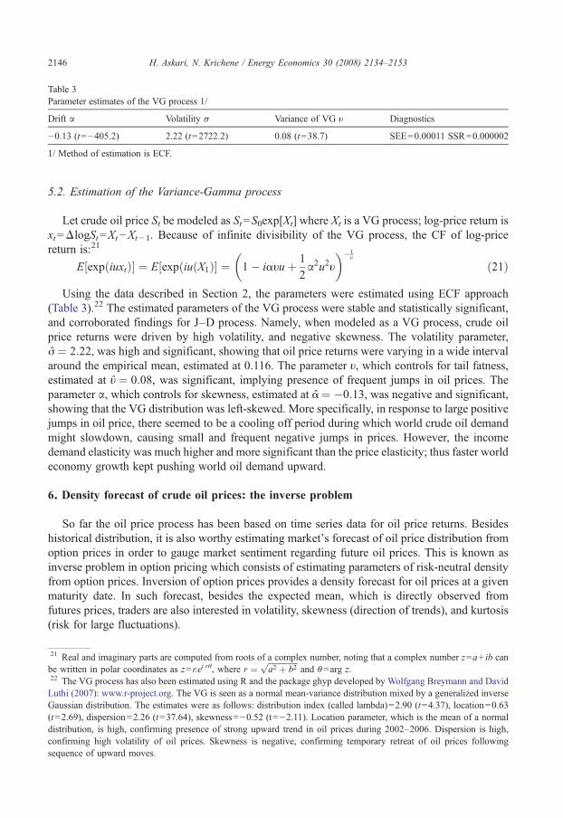
Table 3Parameter estimates of the VG process 1/

Drift α Volatility σ Variance of VG υ Diagnostics

−0.13 (t=−405.2) 2.22 (t=2722.2) 0.08 (t=38.7) SEE=0.00011 SSR=0.000002

1/ Method of estimation is ECF.


5.2. Estimation of the Variance-Gamma process

Let crude oil price St be modeled as St=S0exp[Xt] where Xt is a VG process; log-price return isxt=ΔlogSt=Xt−Xt− 1. Because of infinite divisibility of the VG process, the CF of log-pricereturn is:21

E exp iuxtð Þ½ � ¼ E½exp iu X1ð Þð � ¼ 1� iαυuþ 12α2u2υ

� ��1υ

ð21Þ

Using the data described in Section 2, the parameters were estimated using ECF approach(Table 3).22 The estimated parameters of the VG process were stable and statistically significant,and corroborated findings for J–D process. Namely, when modeled as a VG process, crude oilprice returns were driven by high volatility, and negative skewness. The volatility parameter,σ¼ 2:22, was high and significant, showing that oil price returns were varying in a wide intervalaround the empirical mean, estimated at 0.116. The parameter υ, which controls for tail fatness,estimated at υ¼ 0:08, was significant, implying presence of frequent jumps in oil prices. Theparameter α, which controls for skewness, estimated at α¼ �0:13, was negative and significant,showing that the VG distribution was left-skewed. More specifically, in response to large positivejumps in oil price, there seemed to be a cooling off period during which world crude oil demandmight slowdown, causing small and frequent negative jumps in prices. However, the incomedemand elasticity was much higher and more significant than the price elasticity; thus faster worldeconomy growth kept pushing world oil demand upward.

6. Density forecast of crude oil prices: the inverse problem

So far the oil price process has been based on time series data for oil price returns. Besideshistorical distribution, it is also worthy estimating market's forecast of oil price distribution fromoption prices in order to gauge market sentiment regarding future oil prices. This is known asinverse problem in option pricing which consists of estimating parameters of risk-neutral densityfrom option prices. Inversion of option prices provides a density forecast for oil prices at a givenmaturity date. In such forecast, besides the expected mean, which is directly observed fromfutures prices, traders are also interested in volatility, skewness (direction of trends), and kurtosis(risk for large fluctuations).

21 Real and imaginary parts are computed from roots of a complex number, noting that a complex number z=a+ ib canbe written in polar coordinates as z= r.ei.rθ, where r ¼ ffiffiffiffiffiffiffiffiffiffiffiffiffiffiffi

a2 þ b2p

and θ=arg z.22 The VG process has also been estimated using R and the package ghyp developed by Wolfgang Breymann and DavidLuthi (2007): www.r-project.org. The VG is seen as a normal mean-variance distribution mixed by a generalized inverseGaussian distribution. The estimates were as follows: distribution index (called lambda)=2.90 (t=4.37), location=0.63(t=2.69), dispersion=2.26 (t=37.64), skewness=−0.52 (t=−2.11). Location parameter, which is the mean of a normaldistribution, is high, confirming presence of strong upward trend in oil prices during 2002–2006. Dispersion is high,confirming high volatility of oil prices. Skewness is negative, confirming temporary retreat of oil prices followingsequence of upward moves.

http://www.r-project.org


Assuming a VG distribution for log-price, the inverse problem can be stated as findingparameters θ=(α, σ, υ) satisfying σ≥0, by minimizing the quadratic pricing error:

h ¼ argminh

1M

XMj¼1

C*j T ;Kj

� �� Cj T ;Kj

� � 2; j ¼ 1; 2; N :;M ð22Þ

Subject to put-call parity constraint:

S0 þ Pj T ;Kj

� �� C*j T ;Kj

� � ¼ Kje�rT

where Cj⁎(T,Kj) denotes call option price computed from VG distribution, Cj (T,Kj) and Pj (T,Kj)

denote, respectively, market call and put option prices for maturity T and strikes Kj, S0 asset priceat t=0, r risk-free interest rate, and M denotes number of traded options (or strikes). Put-callparity condition brings extra-sample information which helps to regularize the estimationproblem.23 Choosing a penalty parameter ℓ≥0, minimization problem becomes:

h ¼ argminh

1M

XMj¼1

C*j T ;Kj

� �� Cj T ;Kj

� � 2þS S0 þ Pj T ;Kj

� �� C*j T ;Kj

� �� Kje�rT

2� �ð23Þ

The above minimization requires knowledge of functional form of Cj⁎(T,Kj). If the transitiondensity of the process is known in closed form, then Cj⁎(T,Kj) can be derived as discountedexpected payoff under a risk neutral density, namely:

C*j T ;Kj

� � ¼ E max ST � Kj; 0� �� ð24Þ

However, noting that many LPmay not have a density function in closed form, or have a densityfunction which is not easily tractable, Carr andMadan (1999), and Lewis (2001) suggested the useof methods based on CF of a stochastic process to price options in the Fourier space. Assuming CFis known analytically, Carr and Madan (1999) proposed Fast Fourier transform (FFT) method tocompute option prices. They showed that option price can be written as:

C*j T ;Kj

� � ¼ exp �akj� �p

Z l

0Re e�iukjwT uð Þ� �

du ð25Þ

Where ψT (u) is Fourier transform of a modified call option price, u transform variable, kj=logKj, T maturity date. In fact, defining the modified call option as: cT (k)≡exp(ak)CT (k) foraN0, k=log K, its Fourier transform can be written as wT uð Þ ¼Rl�leiukcT kð Þdk. Carr and Madan(1999) showed that ψT (u) can be expressed in terms of CF of the risk-neutral density ϕT (u) as:

wT uð Þ ¼ e�rT/T u� aþ 1ð Þið Þa2 þ a� u2 þ i 2aþ 1ð Þu ð26Þ

23 Cont and Tankov (2004b) argued that inverse problem is an ill-posed problem and proposed relative entropy, which isthe Kullback–Leibler distance for measuring proximity of two equivalent probability measures, as a regularizationmethod with prior distribution estimated from statistical data via maximum likelihood method. This regularization willresult in a unique martingale measure.


For aN0, singularity at u=0 disappears. The option price can therefore be computed by FFTprovided ϕT(− (a+1)i) is finite. For the VG model, Madan et al. (1998) showed that the CF forlog of sT is:

/T uð Þ ¼ exp log S0ð Þ þ r þ xð ÞT½ � 1� iαυuþ 12σ2u2υ

� ��Tυ

ð27Þ

where S0 is asset price at t=0, x ¼ 1υ

� �ln 1� αυ� 1

2σ2υÞ�

, and θ=(α, σ, υ) are from historicaldensity.

Estimation of implied risk-neutral distribution from option prices is a deconvolution problem.Madan et al. (1998) applied maximum likelihood method to density function to calibrate aVariance-Gamma process based on option prices. In this section, deconvolution methods based onCF are applied as CF necessarily satisfies the same differential equations or least squaresproblems as corresponding option prices. The estimation relies principally on ECF method. Theleast squares are restated in Fourier space as:

h ¼ argminh

1

N

XNi¼1

wT uið Þ � 1

M

XMj¼1

euikj eakjCj T ;Kj

� � !2

þS S01

M

XMj¼1

euikj eakj þ 1

M

XMj¼1

euikj eakjPj T ;Kj

� �� wT uið Þ � e�rT

M

XMj¼1

euikj eakjKj

!2

0BBBBB@

1CCCCCA

ð28Þ

i=1,2,....,N; where N is grid size in Fourier space. Expression for ψT (u) was given above.To assert robustness of estimated parameters, an alternative calibration method was applied.

Let V=(C1,....,CM, P1,.....,PM) be a (2M,1) vector of market call and put option prices, let D be apayoff matrix with dimensions (2M, NS) where NS≥M is number of states. V is related toempirical risk-neutral distribution, q, as follows:24

V ¼ e�rT � D � q ð29Þ

Risk-neutral distribution is computed using Inquiries to Tikhonov regularization methoddescribed in Engel et al. (2000) as:25

q ¼ erT � DVDþ j � Ið Þ�1�DV� V ð30Þ

Where κN0 is a penalty parameter. Knowledge of q enables to estimate parameters using ECFmethod. Define states at time T as ST

j, j=1,2,…,NS, and NS is number of states at time T; each state

24 This equation can be restated with a view to using the call-put parity condition. Let DC (M, NS) and Dp (M, NS) be thepayoff matrices associated with call and put options respectively; let also, VC=(C1,…,CM)′ and Vp=(P1,…,PM) beobserved call and put option prices, VK be a vector of strikes, and V1= (1,…,1)′ be the unit vector, then: VC=e

-rt×DC.qsubject to: S0V1+Vp−e− rt×DC.q=e− rtVK.25 Computation of q was carried out using the Matlab package by C. Hansen (1998): Regularization Tools A MatlabPackage for Analysis and Solution of Discrete Ill-Posed Problems.


is related to log-price returns XTj by ST

j=F0TeXT

j

,26 where F0T is futures price at t=0 for delivery at

T. Define ECF as:

/n uð Þ ¼R

eiuXT fn xð Þdx ¼XNS

j¼1

exp iuX jT

� �qj ¼

XNS

j¼1

cos uX jT

� �qj þi

XNS

j¼1

sin uX jT

� �qj ð31Þ

and theoretical CF ϕVG(u) as given in Eq. (21), ECF is accordingly stated as:

h ¼ argminh

1N

XNi¼1

/n uið Þ � /VG uið Þð ÞVW /n uið Þ � /VG uið Þð Þ; i ¼ 1; 2; N ;N ð32Þ

Where W is a positive semi-definite weighting matrix.The inverse problem was applied for the VG model only because of space limitation. The

same methodology applies identically to the J–D model.27 The observed data set was for July21, 2006; it consisted of call and put futures options contracts maturing end-September 2006;the risk-free interest rate, taken here to be the three-month US Treasury bill rate, was equal to4.965; and the crude futures price, was equal to US$74.43/barrel. The constrained minimizationyielded the following triplet for the risk-neutral distribution: σ2 ¼ 1:72, υ¼ 1:12, α¼ 0:37which described market’s expectations on July 21, 2006 regarding futures prices end-September 2006. The alternative method yielded similar estimates: σ2 ¼ 1:90, υ¼ 1:05, α¼0:34. Clearly, market participants did not anticipate any short-term change in underlyingfundamentals characterizing oil markets. They expected oil prices to remain highly volatile(σ2 ¼ 1:72) and dominated by a jump process (υ¼ 1:12). They also expected oil prices toremain under pressure, as they assigned higher probabilities for oil prices to rise above thefutures price level than to fall below this level. This was indicated by a right-skewed risk-neutral distribution (α¼ 0:37).

7. Conclusions

Oil price dynamics is relevant for hedging, forecasting, and making policy. Our main findingsare that these dynamics are dominated by strong upward drift and frequent jumps, causing oilmarkets not to settle around a mean. While oil prices attempted to retreat following major upwardjumps, there was a strong positive drift which kept pushing these prices upward. Volatility washigh, making oil prices very sensitive to small shocks and to news. The findings for both the J–D

27 The risk-neutral CF for any asset price model is given: E[exp(iu log(S(t)))]=exp(iu((log S(0)+ rt− log E[exp(X(t)])E[exp(iuX(t))]. For the J–D model, the resulting risk-neutral process for the asset price is:

/T uð Þ ¼ exp ln S0ð Þ þ r þ xð ÞT½ �exp T �σ2u2

2þ iAuþ k exp ibu� d2u2

2

� �� 1

� �� ; where

x ¼ σ2

2þ Aþ k exp bþ d2

2

� �� 1

� �� :

26 Probability density for XTj is the same as probability density for ST

j. Indeed, if x is a random variable with probabilitydensity f (x), for a monotone change of variable y=g(x), the probability density of y, denoted h(y), is given by h yð Þ ¼j 1g Vg�1 yð Þð Þ jf g�1 yð Þð Þ where g−1 is inverse function of g and g′ is derivative. For STj=F0e

XT, the factor j 1g Vg�1 yð Þð Þ j is equal to 1.


and VG specification were fully consistent with underlying fundamentals for oil markets andworld economy. More specifically, faster world economic growth during the sample period andhighly expansionary monetary policies caused demand for crude oil to expand at a similar pace.Given price inelastic oil demand and supply, any small excess demand (supply) would require alarge price increase (decrease) to clear oil markets; hence, the observed high intensity of jumpsand the strong stimulus for oil prices to rise.

When modeled as a jump–diffusion (J–D) process, oil price dynamics were dominated bythe discontinuous Poisson jump component compared to the continuous Gaussian diffusioncomponent, showing that oil markets were sensitive to demand and supply shocks and to news.While the variance of the diffusion component was high and significant, it was surpassed by astill higher and significant variance of the jump component. Both variances, together, illustratedthe high volatility of the oil markets. The drift of the diffusion component was, however, veryhigh and significant, indicating that oil prices were strongly influenced by an upward trend. Themean of the jump component was negative; more specifically, sharp upward jumps in oil priceshad a temporary restraining effect on oil demand and were followed by a short-lived sequenceof price declines. The mean of the jump component was, however, outweighed by the drift ofthe diffusion component, which kept prices on a rising trajectory.

Oil prices were also modeled as a Levy process (LP) with a variance-gamma (VG)distribution. The findings were similar to the J–Dmodel. The variance of the VG distribution wassignificant and high. The parameter controlling for the jump process was significant, indicatingthat oil prices were influenced by the jump component. The skewness of the VG distribution wasnegative, indicating that large upward moves in oil prices triggered a temporary depressing effecton world oil demand, translating into a temporary sequence of small negative jumps in oil prices.However, the upward momentum outweighed the small negative jumps. Turning to marketexpectations, the implied risk-neutral distribution from call and put option prices, assuming a VGprocess, showed that market participants held higher probabilities for oil prices to rise, than tofall, above the futures price, and expected oil prices to remain volatile and dominated by a jumpprocess.

Our findings are relevant for policymakers and industry analysts. The results establish thenature of the stochastic process underlying oil prices and the importance of the componentsdriving this process. Process parameter estimates could be seen to convey the effect ofexpansionary macroeconomic policies on oil prices during the sample period. A change inprocess parameters would require a change in underlying macroeconomic fundamentals. Ouralternative modeling approaches are highly relevant for forecasting, risk management, derivativespricing, and gauging the market’s sentiment. Our findings should be also helpful for developingand monitoring policies for stabilizing oil markets.

7.1. Annex: method of cumulants of probability distributions

Suppose that X is a real random variable whose real moment generating function is defined asM uð Þ ¼ E euXð Þ ¼Rl�leuX f Xð ÞdX , where f (X) is the probability density of X. Just as the momentgenerating function M of X generates its moments, the logarithm of M generates a sequenceof numbers called cumulants. The cumulants κn of the probability density of X are given byM uð Þ ¼ E euXð Þ ¼ 1þPl

n¼1

mnun

n! ¼ expPln¼1

jnun

n!

� �.

Where mn=E(Xn) is the moment of order n of X. The left-hand side of this equation is the

moment-generating function, so κn/n! is the nth coefficient in the power series representation of


the logarithm of the moment-generating function. The logarithm of the moment-generatingfunction is therefore called the cumulant-generating function, written as:28 log M uð Þð Þ ¼ Pl

n¼0

jnun

n! . Themethod of cumulants attempts to recover a probability distribution from its sequence ofcumulants. In some cases no solution exists; in some other cases a unique solution, or more thanone solution, exists. The relationship between moments and cumulants is of paramountimportance in the estimation of the unknown parameters of the density function. First, considermoments about 0, which can be written as mj=E(X

j), j=0,1,2… The cumulant/moment theoremsays that if X is a random variable with nmoments m1, m2,…,mn, then X has n cumulants κ1, κ2,…,κn, and the cumulants are related to the moments by the following recursion formula:29

jn ¼ mn �Pn�1

j¼1n� 1j� 1

� �jnmn�j.

Note that m0=1. By carrying the recursion formula, the relation between raw moments andcumulants can be stated as:

m1 ¼ j1m2 ¼ j2 þ m1j1m3 ¼ j3 þ 2m1j2 þ m2j1m4 ¼ j4 þ 3m1j3 þ 3m2j2 þ m3j1

For central moments, defined by mj=E((X−E(X))j), the first moment m1 is zero; therelationship between moments and cumulants simplifies to:

m1 ¼ j1 ¼ 0m2 ¼ j2m3 ¼ j3m4 ¼ j4 þ 3 m2 j2

The first cumulant is simply the expected value; the second and third cumulants arerespectively the second and third central moments (the second central moment is the variance);but the higher cumulants are neither moments nor central moments, but rather more complicatedpolynomial functions of the moments. The nth moment mn is an nth-degree polynomial in thefirst n cumulants. Of particular interest is the fourth-order cumulant, called kurtosis, which can beexpressed as kurt (X)=E(X4)−3(E(X2))2. Kurtosis can be considered as a measure of the non-Gaussianity of X. For a Gaussian random variable, kurtosis is zero; it is typically positive fordistributions with heavy tails and a peak at zero, and negative for flatter densities with lighter tails.

References

Askari, H., Krichene, N., 2007a. World Crude Oil Markets: Monetary Policy and the 2004–05 Oil Shock. Working Paper,George Washington University Center For The Study of Globalization.

Askari, H., Krichene, N., 2007b. A Short-run Oil and Gas Model Incorporating Monetary Policy. Working Paper, GeorgeWashington University Center For The Study of Globalization.

Bakshi, G., Cao, C., Chen, Z., 1997. Empirical performance of alternative pricing models. Journal of Finance 52,2003–2049.

28 The cumulants are also equivalently defined in terms of the characteristic function, which is the Fourier transformof the probability density function: / uð Þ ¼ E eiuXð Þ ¼ Rl�l eiuX f Xð ÞdX . The cumulants κn are then defined as

ln/ uð Þ ¼ Pln¼1

jniuð Þnn! .

29 This recursion formula is the Faa di Bruno's formula, equivalently written as:mrþ1 ¼Prj¼0

rj

mjjrþ1�j for r=0,…, n−1.


Ball, C.A., Torous, W.N., 1983. A simplified jump process for common stock returns. Journal of Financial andQuantitative Analysis 18, 53–65.

Ball, C.A., Torous, W.N., 1985. On jumps in common stock prices and their impact on call option pricing. Journal ofFinance 40 (1), 155–173.

Bates, D.S., 1996. Jumps and stochastic volatility: exchange rate processes implicit in Deutsche mark options. Review ofFinancial Studies 9 (1), 69–107.

Beckers, S., 1981. A note on estimating the parameters of the diffusion–jump model of stock returns. Journal of Financialand Quantitative Analysis 16 (1), 127–140.

Black, F., Scholes, M., 1973. The pricing of options and corporate liabilities. Journal of Political Economy 81, 637–654.Breymann, W., Luthi, D., 2007. ghyp: A package on generalized hyperbolic distributions. www.r-project.org.Carmona, R., Ludkovski, M., 2005. Spot Convenience Yield Models for Energy markets. Working Paper.Carr, P., Madan, D., 1999. Option valuation using fast Fourier transform. Journal of Computational Finance 2, 61–73.Carr, P., Wu, L., 2004. Time-changed levy processes and option pricing. Journal of Financial Economics 71, 113–141.Carr, P., Geman, H., Madan, D., Yor, M., 2002. The fine structure of asset returns: an empirical investigation. Journal of

Business 75 (2), 305–332.Carr, P., Geman, H., Madan, D., Yor, M., 2003. Stochastic volatility for levy processes. Mathematical Finance 13 (3),

345–382.Casassus, J., Collin-Dufresne, P., 2005. Stochastic convenience yield implied from commodity futures and interest rates.

Journal of Finance 60 (5), 2283–2331.Chacko, G., Viceira, L.M., 2003. Spectral GMM estimation of continuous-time processes. Journal of Econometrics 116,

259–292.Clark, P.K., 1973. A subordinated stochastic process with finite variance for speculative prices. Econometrica 41,

135–155.Cont, R., Tankov, P., 2004a. Financial Modeling with Jump Processes. Chapman & Hall/CRC.Cont, R., Tankov, P., 2004b. Non-parametric calibration of jump–diffusion option pricing models. Journal of

Computational Finance 7 (3), 1–49.Das, S.R., Sundaram, R.K., 1999. Of Smiles and Smirks: A Term Structure Perspective. Journal of Financial and

Quantitative Analysis 34 (2), 211–239.Duffie, D., Pan, J., Singleton, K., 2000. Transform Analysis and Asset Pricing for Affine Jump–Diffusion Models.

Econometrica 69 (6), 1343–1376.Engel, H.W., Hanke, M., Neubauer, A., 2000. Regularization of Inverse Problems. Kluwer Academic Press.Fama, E.F., 1965. The behavior of stock market prices. Journal of Business 34, 420–429.Feuerverger, A., 1990. An efficiency result for the empirical characteristic function in stationary time-series models. The

Canadian Journal of Statistics 18 (2), 155–161.Feuerverger, A., Mureika, R.A., 1977. The empirical characteristic function and its applications. The Annals of Statistics

5 (1), 88–97.Feuerverger, A., McDunnough, P., 1981a. On some Fourier methods for inference. Journal of the American Statistical

Association 78 (375), 379–387.Feuerverger, A., McDunnough, P., 1981b. On the efficiency of empirical characteristic function procedures. Journal of the

Royal Statistical Society, Series B 43 (1), 20–27.Gibson, R., Schwartz, E.S., 1990. Stochastic convenience yield and the pricing of oil contingent claims. Journal of Finance

45 (3), 959–976.Hamilton, J.D., 1983. Oil and the macroeconomy since World War II. Journal of Political Economy 91, 228–248.Hansen, L., 1982. Large sample properties of generalized method of moments estimators. Econometrica 50, 1029–1054.International Energy Agency, 2006. Oil Market Report. September.International Monetary Fund, 2006. World Economic Outlook. September.Jorion, P., 1988. On jump processes in the foreign exchange and stock markets. The Review of Financial Studies 1 (4),

427–445.Kendall, M., Stuart, A., 1977. The Advanced Theory of Statistics. MacMillam Publishing Company, New York.Lewis, A., 2001. A simple option formula for general jump-diffusion and other exponential levy processes. Envision

Financial Systems and Option City. Net.Madan, D.B., Seneta, E., 1987. Simulation of estimates the empirical characteristic function. International Statistical

Review 55 (2), 153–161.Madan, D., Milne, F., 1991. Option pricing with VG martingale components. Mathematical Finance 1, 39–56.Madan, D., Carr, P., Chang, E., 1998. The variance gamma process and option pricing. European Finance Review 2,

79–105.

http://www.r-project.org


Mandelbrot, B., 1963. New methods in statistical economics. Journal of Political Economy 61, 421–440.Merton, R.C., 1976. Option pricing when underlying stock returns are discontinuous. Journal of Financial Economics 3,

125–144.Parzen, E., 1962. On estimation of a probability density function and mode. The Annals of Mathematical Statistics 33,

1065–1076.Pindyck, R.S., 2002. Volatility and Commodity Price Dynamics. Working Paper.Postali, F.A.S., Picchetti, P., 2006. Geometric Brownian motion and structural breaks in oil prices: a quantitative analysis.

Energy Economics 28, 506–522.Prause, K., 1999. The generalized hyperbolic models: Estimation, financial derivatives and risk measurement. PhD Thesis,

Mathematics Faculty, University of Freiburg.Press, S.J., 1967. A compound events model for security prices. Journal of Business 40, 317–335.Schwartz, E., 1997. The stochastic behavior of commodity prices: implications for valuation and hedging. Journal of

Finance 52 (3), 922–973.Schwartz, E., Smith, J.E., 2000. Short-term variation and long-term dynamics in commodity prices. Management Science

46 (7), 893–911.

oil price dynamics (2002 2006) - institut für …bwl.univie.ac.at/.../oilpricedynamics.pdf · ·...

Documents