the dynamics of crude oil price differentials · the dynamics of crude oil price differentials ......

The Dynamics of Crude Oil Price Differentials

Bassam Fattouh

Centre for Financial and Management Studies, SOAS

and

Oxford Institute for Energy Studies

January 2008

1

The contents of this paper are the sole responsibility of the author. They do not necessarily represent the views of the Oxford Institute

for Energy Studies or any of its Members.

Copyright © 2008

Oxford Institute for Energy Studies

(Registered Charity, No. 286084)

This publication may be reproduced in part for educational or non-profit purposes without special permission from the copyright holder, provided acknowledgment of

the source is made. No use of this publication may be made for resale or for any other commercial purpose whatsoever without prior permission in writing from the Oxford

Institute for Energy Studies.

ISBN

978-1-901795-70-7

2

Contents Contents ......................................................................................................................... 2 Abstract .......................................................................................................................... 3 1. Introduction ................................................................................................................ 4 2. Some Features of Crude Oil Price Differentials ........................................................ 7 3. Empirical Method .................................................................................................... 10 4. Data .......................................................................................................................... 11 5. Empirical Results ..................................................................................................... 13

5.1 Dynamics of Price Differential between Crude Oils of Different Quality ......... 13 5.2 Price Differentials between Crude Oils of Similar Quality ............................... 15 5.3 Price Differentials between Crude Oils one of which is Linked to an Active Futures Market......................................................................................................... 16 5.4 Price Differentials between Crude Oils both with Tradable Paper Contract ... 17 5.5 Discussion of the Empirical Results .................................................................. 17

6. Conclusion ............................................................................................................... 18 References .................................................................................................................... 20

Tables Table 1: Pairs of Crude Oil Price Differentials Analysed ............................................ 22 Table 2: Sahara–Maya Price Differential .................................................................... 23 Table 3: Estimation of Threshold Autoregressive Model (Sahara–Maya) .................. 24 Table 4: Bonny–Maya Price Differential ..................................................................... 25 Table 5: Estimation of Threshold Autoregressive Model (Bonny–Maya) .................. 26 Table 6: Sahara–Bonny Price Differential ................................................................... 27 Table 7: Estimation of Threshold Autoregressive Model (Sahara–Bonny) ................. 28 Table 8: Maya–Lloyd Blend Price Differential ........................................................... 29 Table 9: Estimation of Threshold Autoregressive Model (Maya–Lloyd Blend) ......... 30 Table 10: WTI–Maya Price Differential ...................................................................... 31 Table 11: Estimation of Threshold Autoregressive Model (WTI–Maya) ................... 32 Table 12: WTI–Lloyd Blend Price Differential ........................................................... 33 Table 13: Estimation of Threshold Autoregressive Model (WTI–Lloyd Blend) ........ 34 Table 14: WTI–Sahara Price Differential .................................................................... 35 Table 15: WTI–Bonny Price Differential .................................................................... 36 Table 16: Estimation of Threshold Autoregressive Model (WTI–Bonny) .................. 36 Table 17: WTI–Brent Price Differential ...................................................................... 37 Table 18: WTI–Dubai Price Differential……………………………………………..37 Table 19: Estimation of Threshold Autoregressive Model (Dubai–Maya) ................. 38 Figures Figure 1: Behaviour of Crude Oil Price Differential ............................................ 39 Figure 2: Identification of Threshold Regime for Sahara–Maya ............................ 40 Figure 3: Identification of Threshold Regime for Sahara–Bonny .......................... 41

3

Abstract We model crude oil price differentials as a two-regime threshold autoregressive (TAR)

process using Caner and Hansen’s (2001) method. While standard unit root tests, such as the

Augmented Dickey–Fuller (ADF), are inconclusive in some instances on whether oil price

differentials follow a stationary process, the null hypothesis of unit root can be strongly

rejected based on the threshold unit root test, even for crude oils with very different qualities.

Our results also indicate that the adjustment process is different depending on whether one

considers the differentials between crude oils of similar quality or between oils of different

quality and whether a crude oil is part of a complex that involves a highly liquid tradable

futures contract. These findings suggest that the different oil markets are linked and thus, at

the very general level, the oil market is ‘one great pool’. However, differences in the

dynamics of adjustment suggest that within this one great oil pool, oil markets are not

integrated in every time period and, although the presence of an active futures market has

helped make some distant markets more unified, arbitrage across the different markets is not

costless or risk-free.

4

1. Introduction

Despite the wide variety of internationally traded crude oils with different qualities and

characteristics (the 2006 International Crude Oil Market Handbook describes more than 160

traded crude oil streams), many observers consider the world oil market as ‘one great pool’

(Adelman, 1984). Others argues that oil markets are ‘globalized’ in the sense that supply and

demand shocks that affect prices in one region are transferred into other regional markets

(Weiner, 1991). One implication of the globalization thesis is that prices of similar crudes in

different markets should move closely together such that their price differential is more or

less constant. This is in contrast to oil markets being ‘regionalized’ in which oil prices of

similar qualities move independently to each other in response to shocks. Whether the oil

market is one great pool or is regionalized has important implications in terms of energy

policy and market efficiency. For instance, Weiner (1991) argues that the effectiveness of

government policies, such as releasing crude oil from the Special Petroleum Reserve (SPR),

depends to a large extent on whether the impact of such policy action extends to other regions

or remains confined to the US market. In terms of efficiency, Gülen (1999) argues that

regionalization gives rise to arbitrage opportunities across local oil markets and may render

the market inefficient if arbitrage fails to push prices of similar crude oils in different markets

in line with each other.

The empirical evidence on ‘globalized’ oil markets is mixed. Using simple correlation

analysis and a switching regression system, Weiner (1991) finds support for a high degree of

‘regionalization’ across oil markets. More recent empirical studies that use cointegration

methods find that oil prices in different markets move closely together even in short horizons

providing support for the ‘globalization’ hypothesis (Gülen, 1997; 1999). Using an empirical

method that generates estimates of arbitrage costs between regions (called the arbitrage cost

approach), Kleit (2001) finds that oil markets have become more unified, as evidenced by the

reduction in transaction costs over time. Interestingly, though, his results indicate the

existence of important transaction (arbitrage) costs between oil markets. Milonas and Henker

(2001) examine the price differential between Brent and West Texas Intermediate (WTI) and

conclude that the Brent and WTI markets are not fully integrated.

In this paper, we present new evidence in this debate by analysing the dynamic behaviour of

crude oil price differentials. Although prices of various crude oils may evolve independently

for a period of time, their movements are unlikely to deviate very widely such that their price

differential would increase or decrease without bounds and hence we expect the differential to

follow a stationary process. After all, crude oil prices are linked through the cost-of-carry

relationship and any deviation from this relationship would be restored through arbitrage.

5

These dynamics are most likely to be present for crude oils of similar quality and with liquid

futures market such as the Brent–West Texas Intermediate (WTI) complex. Specifically,

Brent and WTI are linked through the following relationship (Kinnear, 2001; Alizadeh and

Nomikos, 2004):

tWTIBRtBR PDCP ,, =++ (1)

where PBR and PWTI are the prices of dated Brent and WTI at time t, CBR represents the

carrying costs which are necessary to transport the physical Brent and include insurance,

losses, custom duty costs, and pipeline tariff, and D is the quality discount (usually 0.30

cents). If the WTI–Brent price differential, adjusted for carrying costs, is greater than zero,

this would open the trans-Atlantic arbitrage window, i.e. refiners in the USA would increase

their imports of Brent and those crude oils priced off Brent. The trans-Atlantic window would

remain open until the price relationship in (1) is attained. The highly liquid futures market in

both Brent and WTI has increased the ability of market participants to trade the WTI–Brent

arbitrage speedily (Kinnear, 2001).

In the absence of transaction (arbitrage) costs, the deviation of the price differential (adjusted

for carrying costs) from zero would always trigger arbitrage. However, as Balke and Fomby

(1997) observe, the existence of adjustment costs or transaction costs implies that movements

towards some long-run equilibrium value do not need to occur instantaneously and in a linear

fashion. This type of discrete adjustment process has been used to describe many economic

phenomena, such as the behaviour of inventories, interest rates, and investment.

We extend this type of discrete adjustment to oil price differentials, especially for those types

of crude oil with different qualities and/or crude oils that are not linked to an active futures

market. Specifically, crude oil price differentials are modelled as a two-regime threshold

autoregressive (TAR) 1 process using Caner and Hansen’s (2001) method. The threshold

approach decomposes the model into different regimes and thus allows the oil price

differential to follow different dynamics, depending on whether the differential is above or

below a certain threshold. These different dynamics could be explained by the existence of

transaction costs. Although persistent deviations from the equilibrium relationship give rise to

arbitrage opportunities, transaction costs may be high enough such that it would not make it

profitable for traders and refineries to exploit available arbitrage opportunities that would

1 In the absence of transaction costs, any deviation, whether negative or positive, of the price differential (adjusted for carrying costs) from zero would trigger arbitrage. This would suggest that we should include two thresholds and three regimes. However, a model with two regimes is more suitable for our purpose since, as we shall see later, in many cases the differential takes either a positive or a negative value. The inclusion of an additional threshold would have been spurious in this context.

6

restore the equilibrium price relationship unless the oil price differential crosses a certain

threshold. These transaction costs may arise due to the fact that as ‘commodities’ trading

times overlap only for a few hours, simultaneous position taking is limited. Also, another

obstacle for integration is that the delivery instruments differ. Furthermore, because the

delivery of the underlying commodity is costly, riskless arbitrage is not possible’ (Milonas

and Henker, 2001, p. 36). These types of obstacles are likely to be more present in arbitraging

crude oil of different quality and not linked to an active futures market.

In this paper, we study the dynamic behaviour of price differentials between various types of

crude oil. Firstly, we examine the behaviour of price differentials between crude oils of

similar quality (light/light or heavy/heavy). For this group, the price differential is expected to

follow a stationary process, although it is possible to find threshold effects such that error-

correction dynamics become stronger if the differential exceeds a certain threshold.

Secondly, we analyse the behaviour of price differentials of crude oils with different qualities

(light/heavy). Since these types of crude oils do not directly compete with each other and

given that refineries are configured to deal with specific types of crude oil, their prices are

likely to evolve independently and hence their price differential may not follow a stationary

process for the entire period under study. However, we argue that these crude oils cannot

diverge from each other in such a way that their price differential would increase or decrease

without bounds. We expect that once the oil price differential crosses a certain threshold,

arbitrage would become profitable, pushing the differential back to below the threshold. For

instance, it could be argued that refineries would be willing to take delivery and process

heavy crude only if the discount to light crudes is large enough to compensate them for

running their refineries on less suitable crudes. Furthermore, if heavy oil is trading at a large

discount to light crude oil, some oil producers may decide to cut supplies of heavy crude,

raising its price and narrowing the price differential. Thus, for pairs of price differentials

between different quality crudes, we expect to find evidence of threshold stationarity such

that below the threshold, arbitrage ‘switches off’, allowing the oil price differential to behave

as a random walk. Adjustment dynamics would only be triggered if the oil price differential

crosses that threshold.

Finally, to explore whether a highly liquid futures market reduces transaction costs by

facilitating arbitrage, we examine the price differentials between various types of crude oils

and WTI, Brent, and Dubai. WTI and Brent have the most liquid contracts on a physical

commodity while Dubai is the only non-light crude that has a contract tradable over the

counter. We expect the dynamics of price differential to differ depending on whether a crude

oil is part of a complex that involves a highly liquid tradable futures contract.

7

This paper reveals the following interesting findings. Firstly, while standard unit root tests,

such as the Augmented Dickey–Fuller (ADF), are inconclusive in some instances as to

whether oil price differentials follow a stationary process, we can strongly reject the null

hypothesis of unit root based on the threshold unit root test which has better power than

standard unit root tests when the underlying process is non-linear (Caner and Hansen, 2001).

These findings do not apply only to crude oils with similar qualities, but more importantly to

crude oils with different qualities. This evidence suggests that oil price differentials cannot

deviate without bounds, providing support for the ‘globalization’ hypothesis.

Secondly, our results indicate that the adjustment process is different depending on whether

one considers the differentials between crude oils of similar quality or between oils of

different quality. For the latter, we find strong evidence of threshold effects in the adjustment

process. Specifically, below an estimated threshold, there is no evidence of stationarity,

suggesting that these oil price differentials follow a random walk in that regime. However,

once the price differential crosses the estimated threshold, there is evidence of mean reversion.

These threshold effects indicate the existence of transaction costs, which is consistent with

Kleit’s analysis (2001). It is also consistent with the conclusion of Milonas and Henker (2001)

in the WTI–Brent context, where they argue that these two markets are ‘not fully integrated

and this cannot be overcome with the operation of riskless arbitrage’.

Finally, our findings suggest that whether one or both of the crude oils is linked to a highly

liquid futures market affect the dynamics of some crude oil price differentials by eliminating

threshold effects. This applies mainly to crude oils of similar quality but in some instances to

crude oils of different quality. These dynamics may reflect the fact that a crude oil with a

highly tradable contract reduces transaction costs and facilitates arbitrage and hence error

correction dynamics would always be present and would not be triggered by threshold effects.

This paper is divided into four further sections. In Section 2, we outline the various features

of crude oil price differentials. In Section 3, we describe the empirical method used. Section 4

describes the data while Section 5 reports and discusses the empirical results. The last section

provides a conclusion.

2. Some Features of Crude Oil Price Differentials

Crude oil is of little use before refining and is traded for its final petroleum products that

consumers demand. The intrinsic properties of the crude oils determine the mix of the final

petroleum products. The two most important qualities of crude oil are viscosity (thickness or

8

density) and sulphur content.2 Crude oils with lower density (referred to as light crude)

usually yield a higher proportion of the more valuable final petroleum products, such as

gasoline and other light petroleum products, by a simple refining process known as

distillation. Light crude oils are contrasted with heavy crude oils that have a low share of light

hydrocarbons and require much more severe refining processes than distillation, such as

coking and cracking, to produce similar proportions of the more valuable petroleum

products.3 Sulphur, a naturally occurring element in crude oil is an undesirable property and

refiners have to make heavy investments in order to remove it from crude oils. Crude oils

with high sulphur content are referred to as sour crudes while those with low content of

sulphur are referred to as sweet crudes. Since the type of crude oil has a bearing on refining

yields, different types of crude oil fetch different prices. Crude oils that yield a higher

proportion of the more valuable final petroleum products and require a simple refining

process (the light/sweet crude variety) usually command a premium over those that yield a

lower fraction of the more valuable petroleum products and require a more severe refining

process (the heavy/sour crude variety).

However, differences in the quality of crude oils are not the only determinant of oil price

differentials and hence differentials are not constant over time. Variation in oil price

differentials can result from non-parallel movement of either the underlying crude oils or both.

These non-parallel movements are possible because each type of crude oil may be influenced

by local conditions. Milonas and Henker (2001) argue that demand for oil has a seasonal

component which is unlikely to affect two types of crude oil in the same way. In addition,

squeezes in some markets can cause the price of lower quality crude to rise sharply in relation

to higher quality crude, causing the differential to switch from positive to negative values.

The variation in oil price differentials can also be driven by changes in the relative demand

for light and heavy final petroleum products, which can feed into the crude market and alter

the price differentials between crude oils.

Figure 1 plots the price differential between WTI, Brent, and Dubai. These varieties represent

the main crude oil benchmarks of the current international oil pricing system.4 Because there

are many varieties of crude oil, buyers and sellers usually price the crude at a discount or a

premium to particular benchmarks. Nearly all oil traded outside the USA and the Far East is

2 Density is usually measured by API degrees (°). Crude oil with high API has a low density and flows freely at room temperature. 3 Not all refiners, however, have the technical capacity to undertake such a complex refining operation. The least complex refineries that use heavy crude will obtain a lower yield of the more valuable light refined products and higher yield of the less valuable heavy refined products, reducing their profit margins. 4 For details see Horsnell and Mabro (1993) and Fattouh (2006).

9

priced using Brent as a benchmark while oil traded to the USA is priced off WTI. Dubai is the

main benchmark for Middle Eastern exports to Asia. WTI is a very high quality crude with

API of 39.6° and contains only about 0.24 per cent of sulphur. Given these qualities, WTI is

considered as light/sweet crude. Brent blend is a combination of crude oil from different oil

fields located in the North Sea. Its API gravity is 38.3° while it contains about 0.37 per cent of

sulphur, making it light/sweet crude oil, but slightly less so than WTI. Dubai’s API gravity is

32° and contains a high sulphur content of around 2 per cent and thus is considered to be of

sour/heavy variety.

Three important features emerge from Figure 1. As expected, sweet/light crude varieties

(WTI and Brent) usually trade at a premium to sour/heavy crude varieties (Dubai). However,

there are few exceptions to this rule where the higher quality crude was trading at a discount

from the lower quality crude. For instance, during September 2000 due to a successful

squeeze of the Brent market, the price of Brent rose almost $3 above that of WTI although

WTI is of better quality than Brent and usually trades at a premium. In 2007, and as a result of

a large build-up of stockpiles driven by purely infrastructure logistics, the WTI price

decoupled not only from the rest of the world, but also from other US regions, particularly

from the US Gulf (Fattouh, 2007). This was reflected in the large differential between the

prices of the two international benchmarks when the discount of WTI to Brent reached more

than $6.50 in April 2007.

The second feature is that the discount of heavy crude oil to light crude oil could in some

occasions reach very high levels. Many observers have highlighted the rise in demand for

light products and inflexibility of refineries as the main factors for the recent widening of

differentials. The refining industry in the past decade or so has lost much of the needed

flexibility given the changes in the structure of demand for its products, the mandated

modification of product specifications and other environmental restrictions, and the changing

mix of its crude slate due to higher incremental volumes of sour and heavier crudes. The

increase in demand for gasoline in recent years and constraints on conversion capacity

resulted in an increase in demand for crude oils that yield a large proportion of gasoline. 5

This widened the differential between light/sweet and heavy/sour crude oils considerably. For

exporters of low quality crude oils, this has important implications on government revenues

5 For most of the past decade returns on investment in refining were quite low, which meant that many refiners were unable to justify significant investment in de-sulphurization. As regulation became law, many refiners chose the easy option of purchasing lower sulphur crude oil feedstocks rather than the option of investing in sulphur-removal facilities. This has pushed refiners to bid up prices of light/sweet crude oils in order to reach the new environmental standards.

10

(Bacon and Tordo, 2005). It also can influence investment decisions by sending strong signals

about the type of refining capacity that the market needs.

The third and most important feature for our analysis is that there has been large variation in

oil price differentials over time, especially in the last two years of the sample. This recent

behaviour of oil price differentials has raised some doubts about whether oil markets have

become more integrated in recent years, especially between crude oils with different qualities.

3. Empirical Method

We model the oil price differential dynamics as a two-regime TAR process. 6 The TAR model

can be written as:

{ } { } tZtZtt uIxIxytt

++=Δ ≥−<− −− λλ θθ11 1

'21

'1 (2)

where t = 1,…, T; xt – 1 = (intpt, yt – 1, Δyt – 1 ,…, Δyt – k)' where y is oil price differential; I(.) is

the indicator function; Zt – 1 is the threshold variable defined as Zt – 1 = yt – m for some m ≥ 1

where m is the delay order 7 ; and ut is an iid mean-zero sequence of error terms. The

deterministic component intpt stands for an intercept; Δyt – j = yt – j – yt – j – 1 is the first order

difference at lag j. The threshold λ is unknown and takes values in the interval λ∈Λ = [λ1, λ2],

where λ1 and λ2 are chosen so that Prob(Zt ≤ λ1) = π1 > 0 and Prob(Zt ≤ λ2) = π2 < 1. 8 It is

convenient to consider the vectors θ1 = (ρ1 β1 α1)' and θ2 = (ρ2 β2 α2)', where ρ1 and ρ2 are

the slopes on the lagged levels, β1 and β2 are the slopes on the deterministic component, and

α1 and α2 are the slopes on the lagged differences in the two regimes.

When estimating the TAR model, for each λ∈Λ, we estimate θ1 and θ2 by Least Squares (LS).

The LS point estimate of the threshold λ̂ is found by minimizing the residual sum of squares.

The corresponding vectors θ̂ 1 and θ̂ 2 are then found by plugging in the point estimate such

that the estimated model can be written as:

6 For details of the empirical method, see Caner and Hansen (2001). The discussion in this section is based on their paper. 7 The delay parameter represents the time lag that it takes the market to respond to deviation from equilibrium. 8 The authors suggest that, setting the bounds of the trimming region to π1 = 0.10 and π2 = 0.90, provides a reasonable trade-off between the power and size properties of the test for threshold effects (see Caner and Hansen, 2001, for details). However, as the authors observe, since this particular choice is somewhat arbitrary, it would be sensible in practical applications to explore the robustness of the results to this choice. Our results are robust in this sense.

11

{ } { } tZtZtt uIxIxytt

ˆˆˆˆ1

'2ˆ1

'1

11++=Δ

≥−<−−− λλ

θθ (3)

To test the null hypothesis of linearity, that is H0: θ1 = θ2, against the alternative of threshold

effects, Caner and Hansen suggest the use of the sup-Wald statistic, WT. The latter is not

identified under the null, and its asymptotic distribution under the assumption of stationary

data was investigated by Davies (1987) and Hansen (1996). Caner and Hansen (2001) find

that under the restriction of a unit root process, the asymptotic distribution of WT depends on

the data structure, which implies that critical values cannot be tabulated, and, therefore, the

authors suggest two bootstrap methods to approximate the asymptotic distribution of WT, one

of which is appropriate for the stationary case while the other is appropriate for the unit root

case. If the true order of integration is unknown, then Caner and Hansen (2001) suggest to

calculate the bootstrap critical values and p-values both ways, and base inference on the more

conservative (larger) p-value.

As for the unit root tests, the following statistics are employed: the two-sided Wald test

statistic, R2T, for the null of unit root, H0: ρ1 = ρ2 = 0, against the alternative H1: ρ1 ≠ 0 or ρ2

≠ 0 and the one-sided Wald test statistic, R1T, for the null of unit root, H0: ρ1 = ρ2 = 0, against

the alternative H1: ρ1 < 0 or ρ2 < 0. Although both statistics have the power to test against the

null of unit root, they cannot discriminate between the stationarity case and the partial unit

root case where the partial unit root case refers to a situation in which the process is stationary

in one regime but has a unit root in the other.

To test for the interesting case of a partial unit root, Caner and Hansen suggest the use of

individual t statistics, t1 and t2 ; t1 tests for the null of unit root, H0: ρ1 = ρ2 = 0, against the

alternative of stationarity only in regime 1, that is, H1: ρ1 < 0 and ρ2 = 0, and the one-sided

Wald test statistic, t2, tests for the null of unit root, H0: ρ1 = ρ2 = 0, against the alternative of

stationarity only in regime 2, that is, H1: ρ1 = 0 and ρ2 < 0. If there are no threshold effects

(unidentified case), the asymptotic distribution of each of the four statistics is found to be

dependent on the data structure. However, asymptotic bounds, free of nuisance parameters

other than the trimming range, are found. Consequently, critical values can be tabulated and

p-values can be computed (Table 3 in Caner and Hansen, 2001). As for the asymptotic

distribution of each of the four statistics in the presence of threshold effects (identified case),

the authors found that the Dickey-Fuller tabulated critical values provide a conservative

bound for the t1 and t2 tests.

4. Data

Given the large variety of crude oils traded in the international market, it is important to limit

our analysis to few crude streams. In this paper, we focus our analysis on the following seven

12

types of crude oils imported into the USA: Nigerian Bonny Light (37º), Algerian Saharan

Blend (44º), Mexican Maya (22º), Canadian Lloyd Blend (22º), West Texas Intermediate

(40º), Brent (38º), and Dubai’s Fateh (32º). This choice of crude oils allows us to examine the

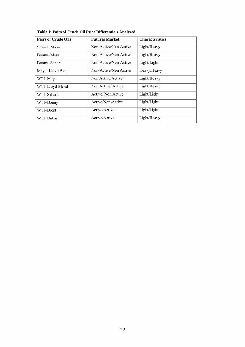
time series properties of the following cases:

• The price differential between crude oils with different quality such as Sahara–Maya

or Bonny–Maya.

• The price differential between crude oils with similar characteristics such as Sahara–

Bonny (light/light) and Maya–Lloyd Blend (heavy/heavy).

Focusing on these differentials allows us to test whether the adjustment process towards the

long equilibrium between crude oils of same quality differs from the adjustment process

between crude oils of different quality. Furthermore, it allows us to test whether prices of

crude oils of very different quality move together such that their price differential is stationary.

Evidence of stationarity would provide stronger support for the globalization hypothesis as it

implies that light and heavy crude oil markets are linked together through arbitrage. Existing

empirical evidence on the behaviour of prices of crude oil of different quality is very thin. The

only exception is Gülen’s (1999) study where he finds that Saudi Arabia heavy crude moves

closely with prices of lighter crude oils in the sub-periods when oil prices have been rising.

The above pairs of crude oil price differentials are not linked to a complex that includes a

futures contract. In order to explore the impact of futures market activity, we also examine the

adjustment process between crude oils that do not have a paper contract (Bonny, Maya,

Sahara, Lloyd Blend) on the one hand and other crude streams that have paper contracts

which are actively traded on the futures market or over the counter (WTI, Brent, and to lesser

extent Dubai). Thus, we also consider the following cases:

• The price differential between pairs of crude oils of similar quality but one of which

has a paper contract that is highly traded on the futures market, such as Sahara–WTI

and Bonny–WTI (light/light).

• The price differential between pairs of crude oils of different quality but one of which

has a paper contract, such as WTI–Maya and WTI–Lloyd Blend (light/heavy).

• The price differential between WTI and Brent, which are of similar quality and are

both actively traded on the futures market.

• The price differential between pairs of crude oils of different quality but both of

which have paper contracts actively traded, namely WTI–Dubai.

13

Table 1 summarizes the 10 pairs of crude oils analysed in this paper. We use weekly data for

the period 1/1/1997 to 26/10/2007 which yield a sample size of 563 observations.9 All the

series were obtained from Energy Information Administration (EIA) and are expressed in US

dollars per barrel. The price differentials are computed as the simple difference between the

prices of the above pairs of crude oils.

5. Empirical Results

The first step in our empirical analysis is to establish whether a price differential is stationary

based on the various unit root tests, namely the Augmented Dickey–Fuller (ADF), Philip–

Perron (1988), and ADF-GLS test developed by Ng and Perron (2001). If evidence of

stationarity based on these unit root tests is found, we do not carry the threshold unit root test

(discussed in step 3 below). On the other hand, if we find evidence of a unit root at this initial

stage, we carry the threshold stationarity test. The power of unit root tests such as ADF is

considerably reduced in the presence of non-linearities and as such standard unit root tests

that do not take into account the possibility of threshold effect and asymmetric adjustment in

oil price differential may reach erroneous conclusions regarding the dynamics of oil price

differentials. In the second step, we test for the linearity of our model using the sup-Wald

statistic, WT. The optimal number of lags is selected using the AIC criterion while the delay

parameter is selected such that the value of sup-Wald statistic, WT, is maximized. This is

equivalent to choosing m that minimizes the residual variance since WT is a monotonic

function of the residual variance. In the third step, we test whether the oil price differential

follows a stationary or a random walk process using the two-sided Wald test statistic, R2T, and

the one-sided Wald test statistic, R1T. In the fourth step, we report the OLS estimates of the

TAR model. We also test for the equality of the coefficients on lagged level and the

coefficients on lagged differences across the two regimes using a joint Wald test. This would

allow us to test which variables are driving the non-linear dynamics in our model.

5.1 Dynamics of Price Differential between Crude Oils of Different Quality

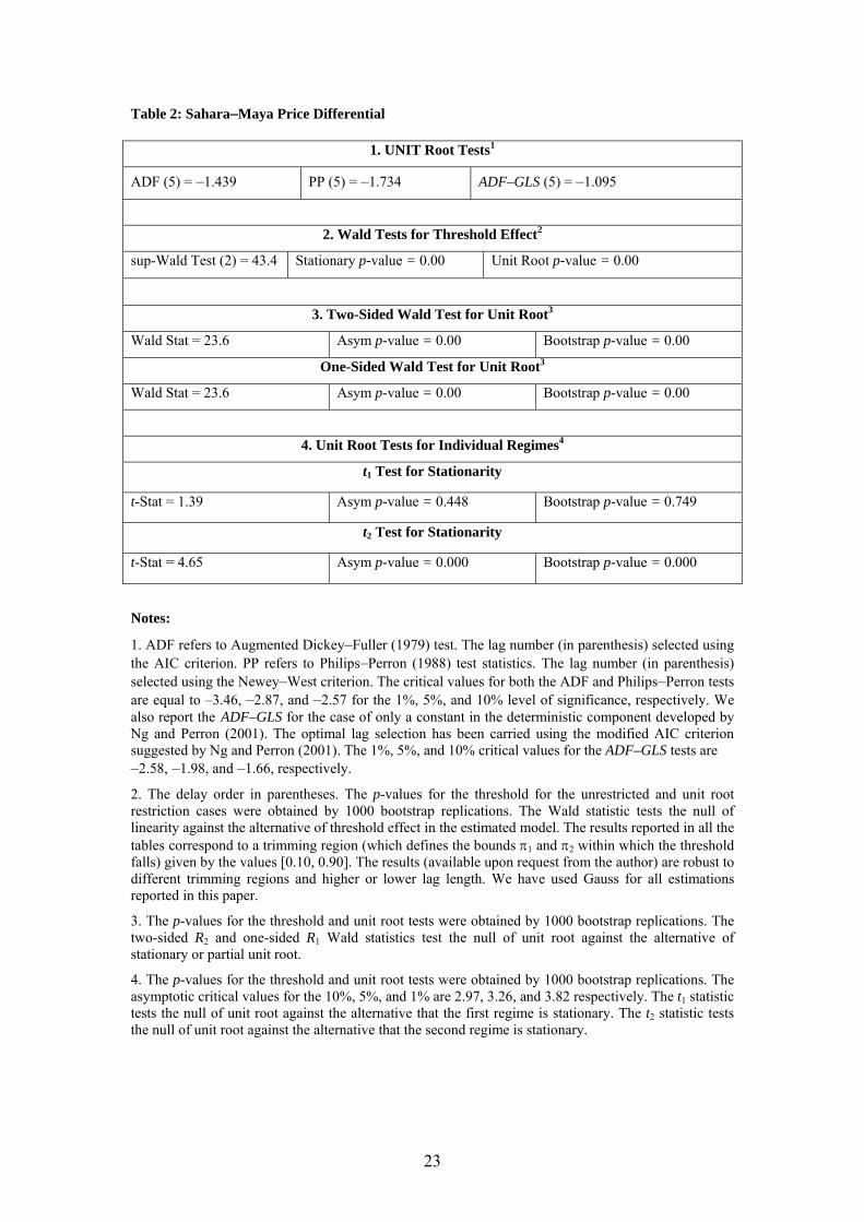
Table 2 reports the results for the Sahara–Maya price differential. As can be seen from the

first part of the table, the various tests indicate that the null of unit root cannot be rejected at

the conventional levels. In part 2 of the Table 2, we report the sup-Wald statistic and the

corresponding bootstrap p-values both for the stationary and unit root cases. As can be seen

from this table, the null hypothesis of linearity against the alternative of threshold effects can

be rejected at the 1 per cent level based on both p-values. We next test whether the oil price

differential follows a stationary or a random walk process using the two-sided Wald test 9 Data on the Canadian Lloyd Blend were discontinued in June 2007 so we augmented the series with Canada’s Heavy Hardisty which has the same API as Lloyd Blend.

14

statistic, R2T, and the one-sided Wald test statistic, R1T (part 3). Both tests clearly indicate that

we can strongly reject the null of unit root at the 1 per cent level. Thus, we can conclude with

confidence that the Sahara–Maya price differential does not have a unit root but contains

threshold effects.

The OLS estimates of the TAR model of lag order p = 5 and delay parameter m = 2 are shown

in Table 3. The threshold estimate is $11.90. In other words, the TAR split the regression

function into two regimes (Regime 1 and Regime 2) depending on whether the lagged value

of the differential lies below or above $11.90. The first regime occurs when the lagged oil

price differential is less than or equal to $11.90. The first regime contains 74.5 per cent of

observations. The second regime, on the other hand, occurs when the oil price differential has

exceeded the $11.90 mark. The TAR estimates reveal some interesting results. They indicate

the existence of an asymmetric adjustment process. While in the second regime there is

evidence of a statistically significant reverting dynamics to the long-run equilibrium as

implied by the statistically significant coefficient on the lagged level, there is no evidence of

such reversion in the first regime. These results are confirmed by the individual one-sided

Wald test statistics, t1 and t2 reported in Table 2 (section 4). They show the existence of a

partial unit root, i.e. oil price differentials process has a unit root process in one regime, but is

stationary in the other. Specifically, the one-sided Wald test statistic t1, indicate that we

cannot reject the null of unit root in favour of the alternative of stationarity in Regime 1. The

one-sided Wald test statistic t2, however, suggests that we can reject the null of unit root in

favour of the alternative of stationarity in Regime 2. The results taken together suggest that

the dynamics of oil price differentials are different depending whether the oil price

differential is below or above the estimated threshold. In the first regime, oil price

differentials follow a random walk process. On the other hand, in Regime 2, oil price

differentials exhibit a stationary behaviour.

It is interesting to note that both the coefficients on lagged levels and the coefficients on

lagged differences are responsible for the non-linearity in our model. This can be tested by a

joint Wald test for the equality of coefficients across the two regimes. As can be seen from

Table 3, the null that the coefficients on yt – 1 are the same can be rejected at the 1 per cent

level, suggesting the difference between the two regimes is due to stationarity versus unit root.

The Wald tests for equality of coefficients on the autoregressive coefficients also indicate that

there are major differences in the coefficients on Δyt – i for many lags (1 ,3, 4, 5) suggesting

that the differences in the autoregressive coefficients are also contributing to the non-linear

dynamics.

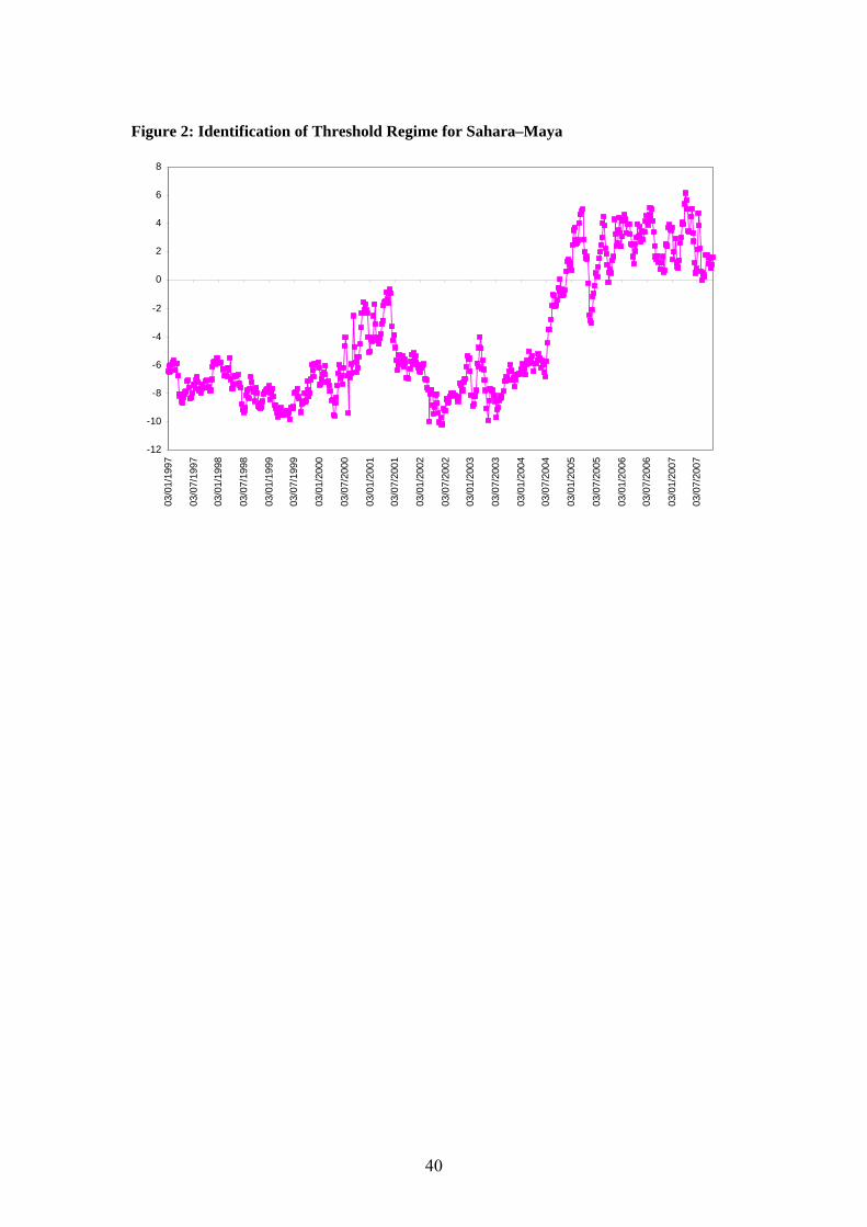
We subtract the price differential from the estimated threshold over the sample period. This

allows us to split observations according to the two regimes, as shown in Figure 2.

15

Specifically, positive values identify the stationary regime while negative values identify the

unit root regime. It is interesting to note that most of the observations in the stationary regime

are concentred in last years of the sample. This is expected as most of the large variations in

oil price differentials occurred in the last three years of the sample.

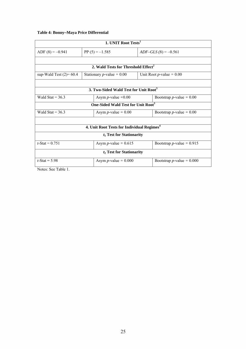
For robustness, in Tables 4 and 5 we report the results for the Bonny–Maya price differential.

The results paint a very similar picture to that of the Sahara–Maya price differential where

unit root tests such as the ADF cannot reject the null of unit root at the 1 per cent level while

the threshold stationary test rejects strongly the null of unit root at the 1 per cent level. The

sup-Wald statistic and the bootstrap p-values for the stationary and unit root cases suggest

that we are able to reject strongly the null of linearity, indicating the existence of threshold

effects. Specifically, the TAR splits the regression function into two regimes depending on

whether the lagged value is below or above $13.30. The TAR estimates indicate the existence

of an asymmetric adjustment process. As before, while in the second regime there is evidence

of a statistically significant reverting dynamics to the long-run equilibrium as implied by the

statistically significant coefficient on the lagged differential, there is no evidence of such

reversion in the first regime. These results are confirmed by the individual one-sided Wald

test statistics, t1 and t2 reported in Table 4 (section 4). The Wald tests for equality of

coefficients on the autoregressive coefficients indicate that both lagged differential and

differences in the autoregressive coefficients (lags 3, 5, and 6) are contributing to the non-

linear dynamics.

5.2 Price Differentials between Crude Oils of Similar Quality

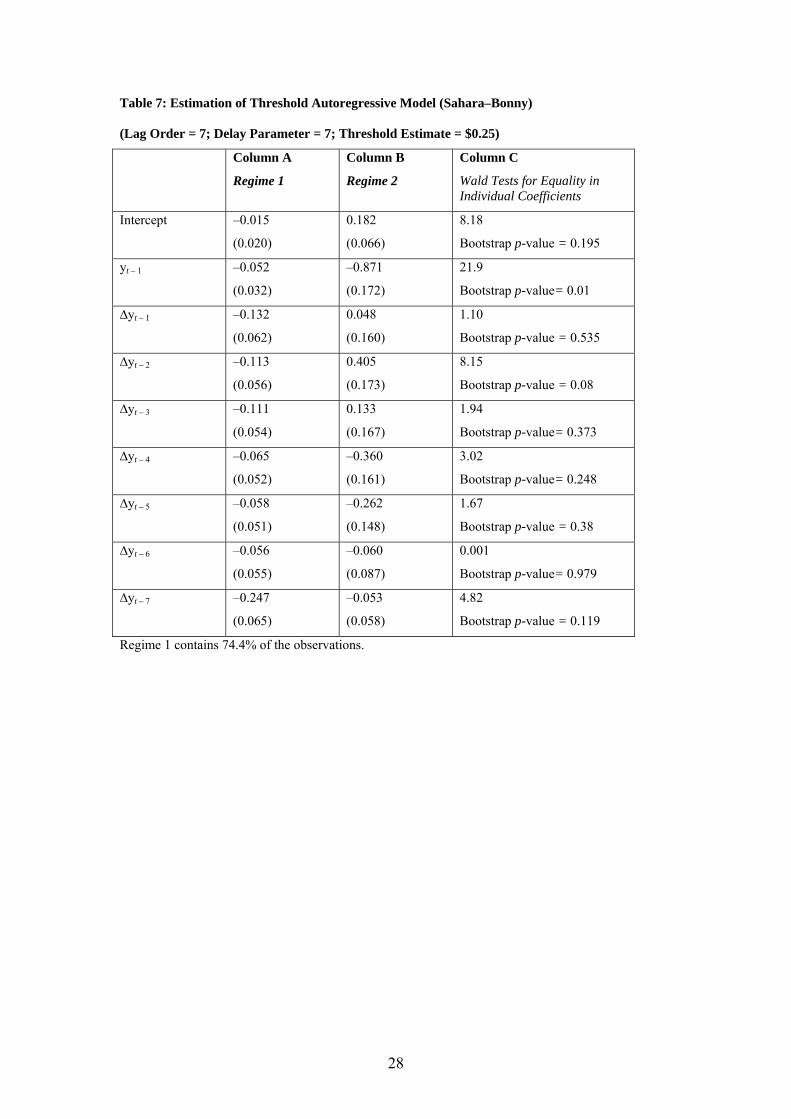
Tables 6 and 7 report the results for the Sahara–Bonny (light/light) price differential. As

expected, the conventional unit root tests suggest that the oil price differential follows a

stationary process and hence we do not carry the threshold unit root test. What is interesting

to note, however, is that the sup-Wald statistic rejects the null of linearity in favour of the

threshold model. The TAR estimates provide support for these threshold effects. Although

both regimes show error correction dynamics (the coefficients on the lagged level are both

significant), these error-correction dynamics become stronger if the differential exceeds the

$0.25 threshold. The Wald tests for equality of coefficients indicate that we can reject the null

that coefficients on the lagged level are equal. The individual Wald test statistics indicate that

the non-linear dynamics are driven by the differences in the coefficients on y t – 1 and not by

the lagged differences. As before, we subtract the price differential from the estimated

threshold over the sample period. This allows us to split observations according to the two

regimes as shown in Figure 3. It is interesting to note that most of the observations in the high

16

error-correcting regime are concentred in last years of the sample although the year 2001–

2002 also contains such observations.

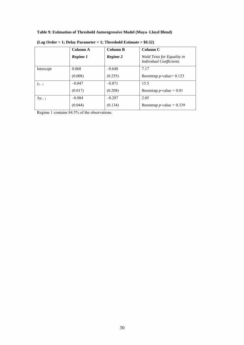
Tables 8 and 9 report the results for the Maya–Lloyd Blend (heavy/heavy) price differential.

As expected, the conventional unit root tests suggest that that the price differential follows a

stationary process. As before, the sup-Wald statistic indicates the rejection of the null of

linearity in favour of the threshold model. The TAR estimates provide support for these

threshold effects. Although both regimes show error correction dynamics (the coefficients on

the lag differentials are both significant), these error-correction dynamics become stronger if

the differential exceeds $0.32. The Wald tests for equality of coefficients indicate that we can

reject the null that coefficients on the lagged level are equal and that the dynamics are driven

by the differences in the coefficients on yt – 1. 10

5.3 Price Differentials between Crude Oils one of which is Linked to an Active

Futures Market

Tables 10 and 11 reports the price differential between WTI and Maya. As can be seen from

Table 10, the tests for unit root indicate that we cannot reject the null of unit root at the 5 per

cent level. Based on the sup-Wald statistic, we are able to strongly reject the null of linearity

in favour of a threshold model based on both bootstrap p-values. Both the two-sided Wald test

statistic, R2T, and the one-sided Wald test statistic, R1T indicate that we can strongly reject the

null of unit root at the 1 per cent level. Thus, we can conclude with that oil price differential

does not contain a unit root. The OLS estimates of the TAR model of lag order p = 3 and

delay parameter m = 3 are shown in Table 11. The threshold estimate is $11.70. The TAR

estimates reveal similar dynamics to the case of Bonny–Maya or Sahara–Maya, indicating the

existence of an asymmetric adjustment process. While in the second regime there is evidence

of a statistically significant reverting dynamics to the long-run equilibrium as implied by the

statistically significant coefficient on the lagged differential, there is no evidence of such

reversion in the first regime. These results are confirmed by the individual one-sided Wald

test statistics, t1 and t2 reported in Table 11, where they reveal the existence of a partial unit

root, i.e. the oil price differentials process has a unit root process in one regime, but is

stationary in the other. For robustness, we also report in Table 12 and 13 the results for WTI–

Lloyd Blend. The results are very similar to the previous ones and hence are not discussed

here.

10 For robustness, we also examined the Maya–Saudi Arabia heavy oil price differential. As expected, we find evidence of stationarity but unlike the Maya–Lloyd Blend price differential, we were not able to reject the null of threshold effects.

17

Table 14 reports the results for the price differential between WTI and Sahara (both light

crude oils). As expected, the conventional unit root tests suggest that we can reject the null of

unit root at the 1 per cent level for both price differentials. What is interesting, though, that

unlike the case of Sahara–Bonny, we do not find any significant threshold effects, indicating

that the adjustment process is linear. For completeness, we also report the results for WTI and

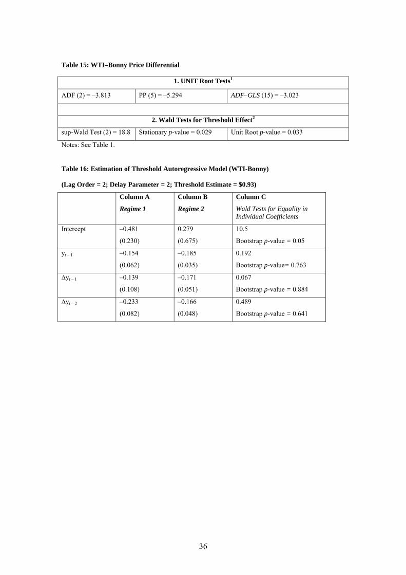
Bonny. As expected, the conventional unit root tests suggest that we can reject the null of unit

root at the 1 per cent level for both price differentials (Table 15). However, unlike the price

differential between WTI and Sahara, we find evidence of threshold effects but, as can be

seen from Table 16, these threshold effects are driven by significant differences in the

constant term rather than differences in lagged levels. In other words, the dynamics of

adjustment are similar in both regimes and do not depend on the price differential reaching a

certain threshold.

The absence of threshold effects in the adjustment dynamics may indicate that price

differentials between pairs of crude oils of similar quality and one of which is linked to a

highly tradable contract reduces transaction costs by facilitating arbitrage and hence the

adjustment process is instantaneous. This tradability aspect, however, does not change the

dynamics when crude oils of different quality are involved.11

5.4 Price Differentials between Crude Oils both with Tradable Paper Contract

Finally, we examine the price differential between crude oils both of which are linked to a

liquid tradable paper contract. We start first with the WTI and Brent price differential. As

expected, the conventional unit root tests, such as the ADF tests, suggest strong evidence of

stationarity. Also, as expected, we find no evidence of threshold effects indicating that the

adjustment process is linear (see Table 17). We next examine the price differential between

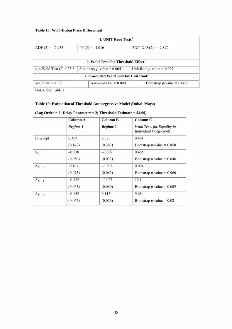
WTI and Dubai, crude oils of different quality. As can be seen from Table 18, we can reject

the null of unit root. But unlike the previous case, we find evidence of threshold effects,

although the non-linear dynamics are driven by the change in the lagged difference (at lags 2

and 3) rather than differences in the adjustment dynamics (see Table 19).

5.5 Discussion of the Empirical Results 11 This conclusion, however, cannot be generalized. For instance, we examined the price differentials between Sahara (light) and Dubai (medium/sour). Dubai is not linked to an active futures market but it is the only available crude that is considered medium (its API is much higher than Maya) and at the same time has a paper contract that is traded over the counter (OTC). Although these crude oils are of different quality, the conventional unit root tests suggest strong evidence of stationarity. Interestingly, the null of linearity in favour of a threshold model cannot be rejected at conventional levels indicating that adjustment to long-run equilibrium is linear. Such evidence strengthens the conclusions that price differentials involving a crude oil with a tradable paper contract can affect price differentials even across crude oils of different quality.

18

Based on the above results, it is possible to draw the following conclusions. Firstly, the price

differential between crude oils of similar quality shows a strong evidence of stationarity.

Secondly, there is strong evidence that the adjustment process between crude oils of similar

quality is very different from that of crude oils of different quality. Our findings indicate that

oil price differentials between crude oils of different quality do not have a unit root. The

results, however, suggest that there are threshold effects in the dynamics of oil price

differentials such that the adjustment process to the long-term equilibrium follows a non-

linear process. For price differentials between crude oils with very different qualities,

reversion to long-run equilibrium occurs only when these price differentials have risen above

a certain threshold. These threshold effects may indicate the existence of transaction costs in

arbitraging crude oil with different qualities and/or transaction costs related to refining

bottlenecks. Specifically, it might be the case that refineries would be willing to take delivery

and process heavy crude only if the discount to light crudes is large enough to compensate

them for running their refineries on less suitable crudes. Thirdly, the existence of a highly

liquid futures market do not alter the first and second conclusion but can change the dynamics

of some crude oil price differentials, especially for crude oils of similar quality by eliminating

the threshold effects. This also extends to crude oils of different quality. For instance, in the

case of the price differential between WTI and Dubai, we find evidence of threshold effects

but these effects are driven by the lagged differences rather than differences in error-

correction dynamics. The absence of threshold effects may indicate that a crude oil with a

highly tradable contract reduces transaction costs by facilitating arbitrage.

6. Conclusion

One of the very interesting features of the oil pricing system in recent years has been the wide

variations in oil price differentials, with the differential reaching very high levels in many

instances. This has raised the issue of whether the oil market should be treated as one great

pool. Using a TAR model suggested by Caner and Hansen (2001) and weekly data on various

pairs of oil price differentials, our findings suggest that oil price differentials follow a

stationary process even for pairs of crude oil with very different qualities. As such, the

different oil markets are linked and thus at the very general level, our findings provide

support for the ‘one great pool’ or ‘globalization’ hypotheses. However, our findings also

suggest that the price differentials between various pairs of crude oil follow very different

dynamics depending on a number of features, such as the types of crude oil and whether a

crude oil is linked to an active futures market. For instance, our findings suggest that the

adjustment process between crude oils of similar quality is very different from that of crude

oils of different quality. While markets for different types of crude oil move together, they are

not fully integrated in every time period. Our evidence of non-linearity in the adjustment

19

process suggests the presences of transaction costs and/or the absence of riskless arbitrage

which may cause oil markets to wander off from each other, but not without bounds. These

differences in the dynamics of crude oil price differentials suggest that within the one great oil

market pool, oil markets are not integrated in every time period and that the regional

influences have not yet disappeared. In addition, although our results indicate that the

presence of an active futures market has helped make some distant markets more unified,

arbitrage across the different markets is not costless or risk-free.

20

References

Adelman, M. A. (1984). ‘International Oil Agreements’. The Energy Journal 5(3): 1–9.

Alizadeh A, N., and Nomikos, N. K. (2004). ‘Cost of Carry, Causality and Arbitrage between

Oil Futures and Tanker Freight Markets’. Transportation Research Part E, Logistics and

Transportation Review 40, No. 4: 297–317.

Bacon, R., and Tordo, S. (2005). Crude Oil Price Differentials and Differences in Oil

Qualities: A Statistical Analysis. Energy Sector Management Assistance Programme

(ESMAP) Technical Paper 081. Washington: World Bank.

Balke, N. S., and Fomby, T. B. (1997). ‘Threshold Cointegration’. International Economic

Review 38: 627–45.

Caner, M., and Hansen, B. E. (2001). ‘Threshold Autoregression with a Unit Root’.

Econometrica 69: 1555–96.

Davies, R. B. (1987). ‘Hypothesis Testing When a Nuisance Parameter is Present Only Under

the Alternative’. Biometrika 74: 33–43.

Dickey, D. A., and Fuller, W. A., (1979). ‘Distribution of the Estimators for Autoregressive

Time Series with a Unit Root’. Journal of the American Statistical Association 74, 427–31.

Energy Intelligence Group (2006). The 2006 International Crude Oil Market Handbook. New

York: Energy Intelligence Group.

Fattouh, B. (2006). ‘The Origins and Evolution of the Current International Oil Pricing

System: A Critical Assessment’. Chapter 3 in R. Mabro (ed.), Oil in the Twenty-First

Century: Issues, Challenges, and Opportunities. Oxford: Oxford University Press.

Fattouh, B. (2007). ‘WTI Benchmark Temporarily Breaks Down: Is It Really a Big Deal?’

Middle East Economic Survey 49, No 20, 14 May.

Gülen, S. G., (1999). ‘Regionalization in the World Crude Oil Market: Further Results’. The

Energy Journal 20(1): 125–39.

Gülen, S. G. (1997). ‘Regionalization in the World Crude Oil Market’. The Energy Journal

18(2): 109–26.

Hansen, B. E. (1996). ‘Inference When a Nuisance Parameter is not Identified Under the Null

Hypothesis’. Econometrica 64: 413–30.

Horsnell, P., and Mabro, R. (1993). Oil Markets and Prices: The Brent Market and the

Formation of World Oil Prices. Oxford: Oxford University Press.

21

Kinnear, K. (2002). ‘The Brent WTI Arbitrage: Linking the World’s Key Crudes’. Energy in

the News, Vol. 2, 2001

Kleit, A. N. (2001). ‘Are Regional Oil Markets Growing Closer Together? An Arbitrage Cost

Approach’. The Energy Journal 22(1): 1–15.

Milonas, N., and Henker, T. (2001). ‘Price Spread and Convenience Yield Behaviour in the

International Oil Market’. Applied Financial Economics 11: 23–36.

Ng, S., and Perron, P. (2001). ‘Lag Length Selection and the Construction of Unit Root Test

with Good Size and Power’. Econometrica 69, 1519–54.

Phillips, P., and Perron, P. (1988): ‘Testing for a Unit Root in Time Series Regressions’.

Biometrica 75: 335–46.

Weiner, R. J. (1991). ‘Is the World Oil Market “One Great Pool?”’ The Energy Journal 12(3):

95–107.

22

Table 1: Pairs of Crude Oil Price Differentials Analysed

Pairs of Crude Oils Futures Market Characteristics

Sahara–Maya Non-Active/Non-Active Light/Heavy

Bonny–Maya Non-Active/Non-Active Light/Heavy

Bonny–Sahara Non-Active/Non-Active Light/Light

Maya–Lloyd Blend Non-Active/Non Active Heavy/Heavy

WTI–Maya Non Active/Active Light/Heavy

WTI–Lloyd Blend Non Active/ Active Light/Heavy

WTI–Sahara Active/ Non Active Light/Light

WTI–Bonny Active/Non-Active Light/Light

WTI–Brent Active/Active Light/Light

WTI–Dubai Active/Active Light/Heavy

23

Table 2: Sahara–Maya Price Differential

1. UNIT Root Tests1

ADF (5) = –1.439 PP (5) = –1.734 ADF–GLS (5) = –1.095

2. Wald Tests for Threshold Effect2

sup-Wald Test (2) = 43.4 Stationary p-value = 0.00 Unit Root p-value = 0.00

3. Two-Sided Wald Test for Unit Root3

Wald Stat = 23.6 Asym p-value = 0.00 Bootstrap p-value = 0.00

One-Sided Wald Test for Unit Root3


4. Unit Root Tests for Individual Regimes4

t1 Test for Stationarity

t-Stat = 1.39 Asym p-value = 0.448 Bootstrap p-value = 0.749



Notes:

1. ADF refers to Augmented Dickey–Fuller (1979) test. The lag number (in parenthesis) selected using the AIC criterion. PP refers to Philips–Perron (1988) test statistics. The lag number (in parenthesis) selected using the Newey–West criterion. The critical values for both the ADF and Philips–Perron tests are equal to –3.46, –2.87, and –2.57 for the 1%, 5%, and 10% level of significance, respectively. We also report the ADF–GLS for the case of only a constant in the deterministic component developed by Ng and Perron (2001). The optimal lag selection has been carried using the modified AIC criterion suggested by Ng and Perron (2001). The 1%, 5%, and 10% critical values for the ADF–GLS tests are –2.58, –1.98, and –1.66, respectively.

2. The delay order in parentheses. The p-values for the threshold for the unrestricted and unit root restriction cases were obtained by 1000 bootstrap replications. The Wald statistic tests the null of linearity against the alternative of threshold effect in the estimated model. The results reported in all the tables correspond to a trimming region (which defines the bounds π1 and π2 within which the threshold falls) given by the values [0.10, 0.90]. The results (available upon request from the author) are robust to different trimming regions and higher or lower lag length. We have used Gauss for all estimations reported in this paper.

3. The p-values for the threshold and unit root tests were obtained by 1000 bootstrap replications. The two-sided R2 and one-sided R1 Wald statistics test the null of unit root against the alternative of stationary or partial unit root.

4. The p-values for the threshold and unit root tests were obtained by 1000 bootstrap replications. The asymptotic critical values for the 10%, 5%, and 1% are 2.97, 3.26, and 3.82 respectively. The t1 statistic tests the null of unit root against the alternative that the first regime is stationary. The t2 statistic tests the null of unit root against the alternative that the second regime is stationary.

24

Table 3: Estimation of Threshold Autoregressive Model (Sahara–Maya)

(Lag Order = 5; Delay Parameter = 2; Threshold Estimate = $11.90)

Column A

Regime 1

Column B

Regime 2

Column C

Wald Tests for Equality in Individual Coefficients

Intercept 0.141

(0.093)

3.30

(0.712)

19.4

Bootstrap p-value = 0.00

yt – 1 –0.022

(0.016)

–0.229

(0.049)

15.9


∆yt – 1 0.097

(0.052)

0.360

(0.077)

7.93


∆yt – 2 –0.058

(0.051)

–0.091

(0.075)

0.131


∆yt – 3 –0.132

(0.050)

0.135

(0.076)

8.45


∆yt – 4 0.122

(0.050)

–0.124

(0.073)

7.57


∆yt – 5 –0.164

(0.050)

0.153

(0.074)

12.4


Regime 1 contains 74.5% of the observations.

25

Table 4: Bonny–Maya Price Differential

1. UNIT Root Tests1

ADF (8) = –0.941 PP (5) = –1.585 ADF–GLS (8) = –0.561


sup-Wald Test (2)= 60.4 Stationary p-value = 0.00 Unit Root p-value = 0.00


Wald Stat = 36.3 Asym p-value =0.00 Bootstrap p-value = 0.00








Notes: See Table 1.

26

Table 5: Estimation of Threshold Autoregressive Model (Bonny–Maya)


Column A

Regime 1

Column B

Regime 2

Column C


Intercept 0.085

(0.092)

5.85

(0.982)

34.2


yt – 1 –0.011

(0.015)

–0.382

(0.063)

31.7


∆yt – 1 0.002

(0.054)

0.213

(0.087)

4.14


∆yt – 2 –0.097

(0.004)

0.111

(0.084)

4.57


∆yt – 3 –0.130

(0.048)

0.200

(0.084)

11.6


∆yt – 4 0.022

(0.048)

–0.010

(0.083)

0.121


∆yt – 5 –0.168

(0.047)

0.173

(0.086)

11.9


∆yt – 6 –0.199

(0.050)

0.085

(0.074)

10


∆yt – 7 0.088

(0.054)

0.027

(0.066)

0.514


∆yt – 8 –0.133

(0.053)

0.002

(0.065)

2.56



27

Table 6: Sahara–Bonny Price Differential

1. UNIT Root Tests1

ADF (7) = –3.046 PP (5) = –7.600 ADF–GLS (7) = –2.732


sup-Wald Test (7)= 111 Stationary p-value = 0.00 Unit Root p-value = 0.00

Notes: See Table 1.

28

Table 7: Estimation of Threshold Autoregressive Model (Sahara–Bonny)


Column A

Regime 1

Column B

Regime 2

Column C


Intercept –0.015

(0.020)

0.182

(0.066)

8.18


yt – 1 –0.052

(0.032)

–0.871

(0.172)

21.9

Bootstrap p-value= 0.01

∆yt – 1 –0.132

(0.062)

0.048

(0.160)

1.10


∆yt – 2 –0.113

(0.056)

0.405

(0.173)

8.15


∆yt – 3 –0.111

(0.054)

0.133

(0.167)

1.94


∆yt – 4 –0.065

(0.052)

–0.360

(0.161)

3.02


∆yt – 5 –0.058

(0.051)

–0.262

(0.148)

1.67


∆yt – 6 –0.056

(0.055)

–0.060

(0.087)

0.001


∆yt – 7 –0.247

(0.065)

–0.053

(0.058)

4.82



29

Table 8: Maya–Lloyd Blend Price Differential

1. UNIT Root Tests1

ADF (1) = –3.971 PP (5) = –4.618 ADF–GLS (1) = –3.506



Notes: See Table 1.

30

Table 9: Estimation of Threshold Autoregressive Model (Maya–Lloyd Blend)


Column A

Regime 1

Column B

Regime 2

Column C


Intercept 0.068

(0.008)

–0.648

(0.255)

7.17


yt – 1 –0.047

(0.017)

–0.871

(0.208)

15.5


∆yt – 1 –0.084

(0.044)

–0.287

(0.134)

2.05



31

Table 10: WTI–Maya Price Differential

1. UNIT Root Tests1

ADF (9) = –1.37 PP (5) = –1.542 ADF–GLS (12) = –0.597












Notes: See Table 1.

32

Table 11: Estimation of Threshold Autoregressive Model (WTI-Maya)


Column A

Regime 1

Column B

Regime 2

Column C


Intercept 0.226

(0.135)

2.19

(1.27)

14.2


yt – 1 –0.030

(0.019)

–0.144

(0.033)

8.56


∆yt – 1 –0.121

(0.060)

–0.074

(0.066)

0.280


∆yt – 2 –0.145

(0.062)

0.0871

(0.064)

6.68


∆yt – 3 0.039

(0.059)

0.042

(0.060)

0.001



33

Table 12: WTI–Lloyd Blend Price Differential

1. UNIT Root Tests1

ADF (7) = –1.321 PP (5) = –2.009 ADF–GLS (7) = –0.787


sup-Wald Test (2)= 57.5 Stationary p-value = 0.00 Unit Root p-value = 0.00







t-Stat = 0.384

Asym p-value = 0.951



t-Stat = 4.07

Asym p-value = 0.004 Bootstrap p-value = 0.007

Notes: See Table 1.

34

Table 13: Estimation of Threshold Autoregressive Model (WTI–Lloyd Blend)


Column A

Regime 1

Column B

Regime 2

Column C


Intercept 0.128

(0.227)

2.71

(0.675)

13.1


yt – 1 –0.010

(0.028)

–0.129

(0.031)

7.82


∆yt – 1 –0.554

(0.068)

–0.079

(0.057)

28.1


∆yt – 2 –0.335

(0.073)

0.170

(0.056)

29.5


∆yt – 3 –0.139

(0.070)

0.008

(0.059)

5.66


∆yt – 4 –0.074

(0.068)

–0.036

(0.057)

0.177


∆yt – 5 –0.066

(0.069)

0.159

(0.057)

6.29


∆yt – 6 –0.103

(0.067)

–0.073

(0.059)

0.110


∆yt – 7 –0.141

(0.062)

–0.093

(0.060)

0.296



35

Table 14: WTI–Sahara Price Differential

1. UNIT Root Tests1

ADF (2) = –4.342 PP (5) = –5.655 ADF–GLS (7) = –3.284



Notes: See Table 1.

36

Table 15: WTI–Bonny Price Differential

1. UNIT Root Tests1

ADF (2) = –3.813 PP (5) = –5.294 ADF–GLS (15) = –3.023



Notes: See Table 1.

Table 16: Estimation of Threshold Autoregressive Model (WTI-Bonny)


Column A

Regime 1

Column B

Regime 2

Column C


Intercept –0.481

(0.230)

0.279

(0.675)

10.5


yt – 1 –0.154

(0.062)

–0.185

(0.035)

0.192


∆yt – 1 –0.139

(0.108)

–0.171

(0.051)

0.067


∆yt – 2 –0.233

(0.082)

–0.166

(0.048)

0.489


37

Table 17: WTI–Brent Price Differential

1. UNIT Root Tests1

ADF (2) = –5.11 PP (5) = –8.737 ADF–GLS (4)= –4.400



Notes: See Table 1.

38

Table 18: WTI–Dubai Price Differential

1. UNIT Root Tests1

ADF (2) = –2.933 PP (5) = –4.016 ADF–GLS (2) = –2.872





Notes: See Table 1.

Table 19: Estimation of Threshold Autoregressive Model (Dubai–Maya)


Column A

Regime 1

Column B

Regime 2

Column C


Intercept 0.357

(0.142)

0.535

(0.243)

0.401


yt – 1 –0.130

(0.050)

–0.089

(0.033)

0.465


∆yt – 1 -0.197

(0.075)

–0.203

(0.063)

0.004


∆yt – 2 –0.332

(0.063)

–0.027

(0.060)

12.1


∆yt – 3 –0.152

(0.064)

0.115

(0.056)

9.68


39

Figure 1: Behaviour of Crude Oil Price Differentials

-10

-5

0

5

10

15

20

03/0

1/19

97

03/0

7/19

97

03/0

1/19

98

03/0

7/19

98

03/0

1/19

99

03/0

7/19

99

03/0

1/20

00

03/0

7/20

00

03/0

1/20

01

03/0

7/20

01

03/0

1/20

02

03/0

7/20

02

03/0

1/20

03

03/0

7/20

03

03/0

1/20

04

03/0

7/20

04

03/0

1/20

05

03/0

7/20

05

03/0

1/20

06

03/0

7/20

06

03/0

1/20

07

03/0

7/20

07

US$

WTI-Dubai WTI-Brent Brent-Dubai

40

Figure 2: Identification of Threshold Regime for Sahara–Maya

-12

-10

-8

-6

-4

-2

0

2

4

6

803

/01/

1997

03/0

7/19

97

03/0

1/19

98

03/0

7/19

98

03/0

1/19

99

03/0

7/19

99

03/0

1/20

00

03/0

7/20

00

03/0

1/20

01

03/0

7/20

01

03/0

1/20

02

03/0

7/20

02

03/0

1/20

03

03/0

7/20

03

03/0

1/20

04

03/0

7/20

04

03/0

1/20

05

03/0

7/20

05

03/0

1/20

06

03/0

7/20

06

03/0

1/20

07

03/0

7/20

07

41

Figure 3: Identification of Threshold Regime for Sahara–Bonny

-4

-3

-2

-1

0

1

2

3

4

5

603

/01/

1997

03/0

7/19

97

03/0

1/19

98

03/0

7/19

98

03/0

1/19

99

03/0

7/19

99

03/0

1/20

00

03/0

7/20

00

03/0

1/20

01

03/0

7/20

01

03/0

1/20

02

03/0

7/20

02

03/0

1/20

03

03/0

7/20

03

03/0

1/20

04

03/0

7/20

04

03/0

1/20

05

03/0

7/20

05

03/0

1/20

06

03/0

7/20

06

03/0

1/20

07

03/0

7/20

07

the dynamics of crude oil price differentials · the dynamics of crude oil price differentials ......

Documents