oil and natural gas reserve prices 1982-2002: implications for
TRANSCRIPT
Oil and Natural Gas Reserve Prices 1982-2002: Implications for Depletion and Investment Cost
by
M.A. Adelman and G.C.Watkins
October 2003
MIT-CEEPR 03-016 WP
Table of Contents Introduction..........................................................................................................................1 I. Mineral Resource Theory – Pertinent Issues .................................................................3
1. Mineral Values and Limited Resources.............................................................3 2. Earlier Data on North American Oil and Gas Reserve Values..........................4 3. The Meaning and Valuation of “Reserves” .......................................................5 4. Values As Marginal Finding-Development Costs .............................................9
II. Review of Transaction Data.........................................................................................11
1. The Scotia Group Database .............................................................................11 2. Description of Transaction Data ......................................................................12
III. Regression Results .......................................................................................................16
1. Results Before Exclusion of Outliers...............................................................18 2. Results Excluding Outliers ..............................................................................19 3. Influence of Reserve Status .............................................................................22 4. Influence of the R/P Ratio................................................................................24 5. Relationship Between Reserve Regression Coefficients and Field Prices..........................................................................................................25 6. Reserve Prices and Company Performance .....................................................26
IV. Reserve Prices, Hotelling Values, Price Expectations, and Returns to Holding……..28
1. Reserve Prices and Hotelling Values – A Comparison ...................................28 2. Oil and Gas Price Expectations........................................................................32 3. Confidence Limits for Price Expectations .......................................................37 4. Mineral Holding Values...................................................................................40
V. Value of U.S. Oil and Gas Reserves ............................................................................43 VI. Concluding Remarks …………………………………………………………………46 References……………………………………………………………………………...…48 Tables & Figures
Table 1: Estimated Market Values of U.S. Oil and Natural Gas Reserves............43 Figure 1: Oil Reserve Prices for 1982-2002 ..........................................................20 Figure 2: Natural Gas Reserve Prices for 1982-2002 ............................................21 Figure 3: Estimates of Hotelling Values and Price Expectations, Oil ...................30 Figure 4: Estimates of Hotelling Values and Price Expectations, Natural Gas .....31 Figure 5a: Implicit Annual Growth Rates for Oil Prices, All Transactions...........34 Figure 5b: Implicit Annual Growth Rates for Natural Gas Prices, All Transactions ...............................................................................................35 Figure 6: Implicit Annual Growth Rates for Oil and Natural Gas Prices, Pure
Transactions ...............................................................................................36
Figure 7: Returns to Holding Oil and Natural Gas Reserves.................................41 Appendix A: Transaction Data ..........................................................................................51
Table A-1: Number of Identified Transactions......................................................52 Table A-2: Summary Statistics for Transaction Values, All Transactions............53 Table A-3: Summary Statistics for Transaction Values, Excluding Outliers ........54 Table A-4: Summary Statistics for Pure Oil Transaction Values, Excluding
Outliers.......................................................................................................55 Table A-5: Summary Statistics for Pure Natural Gas Transaction Values,
Excluding Outliers .....................................................................................56 Table A-6: Summary Statistics for Size of Oil Reserves, All Transactions ..........57 Table A-7: Summary Statistics for Size of Natural Gas Reserves, All Transactions ........................................................................................ 58 Table A-8: Summary Statistics for Transaction Size in Thermal Equivalence,
All Transactions .........................................................................................59 Table A-9: Summary Statistics for Transaction Size in Thermal Equivalence,
Excluding Outliers .....................................................................................60 Appendix B: Estimates of Reserve Prices .........................................................................61
Table B-1a: Regression Results for All Transactions (No Constant) ....................62 Table B-1b: Regression Results for All Transactions (Constant Included)...........63 Table B-1c: Comparisons of Oil Regression Values with Pure Oil Values for
All Transactions (No Constant) .................................................................64 Table B-1d: Comparisons of Natural Gas Regression Values with Pure Gas
Values for All Transactions (No Constant) ...............................................65 Table B-2a: Regression Results for All Transactions (No Constant), Excluding
Outliers (with Robust Standard Errors) .....................................................66 Table B-2b: Regression Results for All Transactions (Constant Included),
Excluding Outliers (with Robust Standard Errors)....................................67 Table B-2c: Effect of Including Constant on Regression Coefficients (Excluding
Outliers) .....................................................................................................68 Table B-2d: Effect of Outliers on Reserve Coefficients (No Constant) ................69 Table B-2e: Comparisons of Oil Regression Values (No Constant) with Pure
Oil Values, Excluding Outliers ..................................................................70 Table B-2f: Comparisons of Natural Gas Regression Values (No Constant) with
Pure Gas Values, Excluding Outliers.........................................................71 Appendix C: Auxiliary Data and Regressions ...................................................................72
Table C-1: Proven Reserves to Production Ratios.................................................73 Table C-2: Regression Results for Transactions with Information on Reserve
Status (No Constant), Excluding Outliers..................................................74 Table C-3: Regression Results for Transactions with Information on R/P Ratios
(No Constant), Excluding Outliers ............................................................75 Table C-4: Oil and Natural Gas Reserve and Field Prices.....................................76 Table C-5: Regression Results of Reserve Price Against Field Price ...................77
Appendix D: Hotelling Values, Implicit Price Expectations and Returns to Holding.......78 Table D-1: Estimates of Hotelling Values and Price Expectations, Oil ................79 Table D-2: Estimates of Hotelling Values and Price Expectations, Pure Oil........80 Table D-3: Estimates of Hotelling Values and Price Expectations, Natural Gas ..81 Table D-4: Estimates of Hotelling Values and Price Expectations, Pure Natural Gas ................................................................................................82 Table D-5: Confidence Limits for Implicit Growth Rates of Oil Prices................83 Table D-6: Confidence Limits for Implicit Growth Rates of Natural Gas Prices .84 Table D-7: Return to Holding Oil and Natural Gas, 1982-2002............................85
1
Oil and Natural Gas Reserve Prices 1982-2002: Implications for Depletion and Investment Cost
M.A. Adelman, Massachusetts Institute of Technology
and G.C. Watkins, University of Aberdeen1
October 2003
Introduction The main object of this research is to estimate a time series for the total and unit value of in-ground proved oil reserves and natural gas reserves in the United States. There are good official statistics of the physical quantities. Our task has been primarily to estimate the in-ground unit values. Total in-ground value equals quantity times unit value.
Such a series has several uses. First, it provides information about the national income and wealth, which includes mineral reserves. About 70 percent of mineral value-added in 1997 was oil and natural gas. [Census Bureau: Manufacturing & Mining] Some such proportion governs mineral wealth in the ground. The U.S. Government itself owns land that includes large reserves. The Bureau of Economic Analysis (BEA) has deplored the lack of reserve price data. They are estimated here.2 Second, there is much interest, when calculating national income and product, to make full allowance for current consumption of minerals. If the oil and gas reserve values are known, capital consumption of minerals is the difference in reserve value from the beginning to the end of the period. This difference can then be partitioned into the difference in physical amount held and the difference in the unit value. Third, there is much interest in the condition of the oil and gas industries in the United States. The value of an in-ground unit (compared with its reproduction cost) is the crucial fact. Unfortunately, we can no longer make this comparison. Since 1991, there has been no compilation of capital expenditures for finding and developing hydrocarbons, formerly published (API 1983-1991; Census ASOG 1973-1982; see
1 The authors are especially grateful to Jie Yang for her skillful and devoted research assistance. We thank Andre Plourde, James Smith and Ralph Kimball for valuable suggestions and comments on an earlier draft. 2 This paper is in part a sequel to an earlier effort: Adelman & Watkins [1996].
7
where: V is the reserve price i is the discount rate on hydrocarbon reserves or production g is the expected annual increase in the net price P embedded in the reserve price,
V.4 This is a more general form of the basic Hotelling equality. That is, if net price rises at the discount rate, i, then g = i, and (3) collapses to V = P. Or, if we could establish by independent evidence that V=P, then it would follow that g = i. But the Hotelling equality V=P has thus far been refuted by the evidence, including evidence presented later in this paper.
Let us now assume that i>g, so that (i-g) is always positive. Then V/P should be an increasing function of ‘a’, at a decreasing rate. The engineering studies bear this out (Bradley¸ op cit). Moreover, since all variables but g are exogenous one can calculate g from them: g = i + a [1- (P/V)] (4). The variable g measures industry expectations of the future course of prices. As might be expected, annual g is highly variable and often negative. In Section IV we estimate the standard error of g.
But although Equation (3) contains some of the same variables as the Hotelling Paradigm, the reserve measure R may be different. In the Hotelling framework, R is exogenous, fixed by nature. In our usage, R measures only oil or gas created by exploration/development investment. The oil or gas is to be produced from defined facilities along some time gradient. R may be increased by later investment. Like many assets, R may be exploited or sold. These uses are substitutes, therefore so are their prices. We attempt to capture the average sales value of a reserve, which equals its average use value.5 National aggregate “proved reserves” in the USA or Western Europe are simply the national aggregate of R. (In most other areas, “proved reserves” are often not even updated, and are no longer useful. Canada has begun to count huge amounts of unhatched chickens – undeveloped reserves - from oil sands.) Such estimates imply little
4 Expression (3) assumes a + i > g, as normally would hold. 5 We acknowledge that sales values may include an element of option value.
8
about the amount of hydrocarbons to be ultimately produced within a given area. That amount cannot be known today, because it depends on future science and technology. “Probable reserves” are the amounts of oil and gas that would be economic to produce given current science and current technology, marked up by some estimate related to further development. “Probable reserves” may be a very useful ordinal measure, permitting one to rank areas where new oil is more likely or less likely to be found [Weeks 1969]. But adding “probable” reserves to current proved reserves adds apples to oranges. The total does not approximate ultimate production. Such a total minus consumption is not an estimate but more confusion. Yet every forecast of exhaustion assumes a total remaining reserve. The crude oil and natural gas industries have diverged. US crude oil production decreased from 9.2 mmbd in 1973 to 5.9 million in 1999, since when it has been approximately constant. Its supply is becoming scarcer in the strict economic sense of the US supply curve moving leftward. (Bradley & Watkins [1994], Adelman [1998], Watkins & Streifel [1998]) This has not been true (perhaps we should say “not yet true”) of natural gas, where North American production and proved reserves grew through the year 2001. For oil, value changes reflect worldwide oil price expectations. For gas, value changes reflect North America gas price expectations.6 Hence, these are two different markets (also see below, section IV-2, “Oil and Gas Price Expectations”). The results of estimating reserve prices for 1982-2002 described in Section III of this paper differ from the earlier Herold series in that they are derived from observed sales of reserve-bearing properties. As with the other series, the current net field price is on average about 4 times the in-ground value for oil and 3 times for gas, and each year’s net field price lies above the regression value plus at least one standard error. This data set cannot be reconciled with the Hotelling Paradigm any more than could the engineering studies or the 1949-1986 set of oil in-ground values. We discuss this further in Section IV. To sum up: the Hotelling theory correctly draws out the implications of its basic assumption: that there exists “an exhaustible natural resource … a fixed stock of oil to divide between two [or more] periods.” [Stiglitz 1976]. Since the implications are false, and the theory is sound, the premise must also be false.
6 But the emerging international market for LNG, with participation by North America suggests that over time the market for natural gas will become a world market.
9
Having found little or no empirical support for the notion of a fixed stock and of the constant increase in reserve values, we can now face a lesser but real problem: what if anything is known about oil and gas becoming more or less scarce over time? 4. Values As Marginal Finding-Development Costs In a competitive industry, the value of reserves of oil or natural gas in-ground is equal to the cost of the marginal reserve added (marginal cost). Even if oil or gas are produced and sold under imperfectly competitive conditions, the addition of reserves is competitive provided there is no public or private restriction upon the associated investment. Restriction was strong in the creation of natural gas reserves before the 1980s, and it was not negligible for crude oil in 1946-1980. The prorationing system in Texas favored investment in high-cost “marginal” wells. Moreover, Federal maximum price-fixing in 1974-1980 favored investment in high-cost “new” oil. These imperfections in the 1948-1986 oil series should (we think) be considered as part of the larger scheme of fluctuations. Some will (not without reason) reject their use. But de-regulation of the oil and natural gas industries in the 1980s abolished constraints, and there are no such uncertainties for 1982-2002. However, there are two principal difficulties in using these data sets to represent long-run cost trends. First, we need to deflate the observations. This would be necessary at any time, but particularly during a period of strong price inflation, as were much of the earlier series and some of 1982-2002. Second, these marginal costs are investment costs. We should not deflate them by a general index of goods bought to satisfy human needs; the appropriate index would be one specific to the particular investment vehicles (equipment and plant) employed. They are investments expected to enjoy a return comparable to investment in other industries, with similar degrees of risk. Indeed, the Hotelling Paradigm is that they should increase at the rate of return on other investments in oil and gas reserves. But if we drop the Paradigm assumption of a fixed hydrocarbon stock, the value of a reserve may vary up or down in any year. In Section IV we test for successive one-period returns from holding oil or gas reserves and find, again, no support for Hotelling patterns. The value of oil reserves is set by competition in the worldwide market for hydrocarbon discovery and development. Part of this market is noncompetitive: in the
10
OPEC countries, investment and output are limited in order to support the price level. Resulting values bear little relation to marginal cost. But the non-OPEC world, which today comprises about 70 percent of world production, and more of worldwide investment, is competitive. It gives a competitive response to an exogenous fact: the fixed price at the field. In non-OPEC areas, discovery and development comprise a sensing/selection network, constantly seeking the cheapest reserves of oil, gas, or both. As we have shown, the series of in-ground values also measures the marginal cost of increasing these reserves. But observed marginal costs are the outcome of a cost function and the position of a demand function. A constant level of observed North American marginal costs may be – and we think is – associated with the supply functions moving leftward – i.e., unfavorably. Therefore more of domestic consumption is supplied by imports. The results presented here are compatible with findings that rising marginal costs have made non-economic more North American deposits. (Bradley & Watkins [1994], Adelman [1998], Watkins & Streifel [1998]) It is the same case as British coal. But the results are not compatible with statements that worldwide discoveries have been declining since the early 1960s. This implies that both discovery and development costs have been increasing. If discovery is yielding smaller, deeper, and farther deposits, they cost more to develop. The IEA discussion is one of the more sober ones. (International Energy Agency, World Energy Outlook 1998, especially pp. 90-100). Yet it is at the least an anomaly that allegedly dwindling discoveries over 40 years have left little trace in in-ground values. In actual fact: there are no precise statistics of oil or gas discoveries. Indeed, it is difficult even to state how to construct one. Merely counting the number of newly listed fields or pools is trivial. The contents of these new fields and pools will not be known until they are fully developed, which may be even as much as a hundred years away. One can at any time estimate those contents, given only the technology of the moment. It is useful comparing the guesses of one year with those of another. In the USA, “discoveries” are a sub-category of development: those reserves developed during the year in newly found fields. In the next year and in all later years, they will be “old” fields. In an area like the Persian Gulf the great bulk of new reserves are created in old fields. Far from indicating scarcity, the development of old fields has been sufficiently cheap as to deter seeking new fields.
11
II. Review of Transaction Data We want to assemble information on the amounts paid for reserves of oil and natural gas to enable us to estimate reserve prices. For a period of twenty or more years, the Scotia Group has been collecting data on reserve related transactions in the US and has sought to identify the value of purchases and sales of reserve assets.7 In what follows below, first we comment on the nature of the Scotia Group transaction data we employ. Second, we examine the Scotia data series, assembled on an annual basis. 1. The Scotia Group Database8
The information in the database is collected entirely from sources in the public domain. The version of the database used has nearly 6000 transactions of which 63 percent have transaction price data and 28 percent have both price and reserve information – the transactions on which we focus.
Some transactions involve non-reserve assets such as pipelines, plants and
equipment, goodwill, strategic elements and the like. “Strategic” acquisitions, especially, may involve significant goodwill. Where values of tangible ancillary assets are known, they have been subtracted from the purchase price; where the purchaser assumes debt, its value is added. The resulting transaction values are referred to as ‘adjusted prices’ in the Scotia database.
Reserves are reported in millions of barrels of oil (mmbbls) and billions of cubic feet of gas (bcf). Producing rates, where available, are reported in thousands of barrels per day of oil (mb/d) and millions of cubic feet of gas per day (mmcf/d). Reserves are treated as proven, developed and on production – unless there were additional information (see below). Buyers and sellers may differ in their reserve assessments, even for proved reserves. However, no such discrepancies were disclosed in the transactions employed. There is no information on expected reserve appreciation that may underlie a given transaction.
International and Canadian transactions are excluded. So are transactions reported in terms of equivalent volumes of oil and gas, but with conversion factors
7 The Scotia Group was founded in 1981 and specializes in the technical and economic analysis of projects, properties and companies. 8 See Scotia Group Documentation “Description and Discussion of the Database” Mimeo, Jan 1995.
12
unknown, individual volumes cannot be derived. Data for some transactions are incomplete, and we exclude them. The database generally excludes stock transactions because reserves cannot be identified.9
Our working assumption, that the reserves changing hands are proved, developed, and producing, is not always true. A transaction could involve non-producing reserves. If so, it may well include reserves normally classified as proved undeveloped or prospective reserves (i.e. probable or possible) even though we have attempted to exclude transactions involving undeveloped reserves from our database.
Suppose parties have included in “reserves” some undeveloped oil or gas
deposits. (Some companies will try to impress the financial community by reporting undeveloped reserves as developed. Some companies overpaying for undeveloped reserves will not be well regarded. We cannot say which event is more probable.) Then the observation we calculate, dollars per barrel-in-ground, will be too low as an estimate of the market value of a barrel of developed reserves. Support now the contrary, that the sellers have lumped undeveloped oil with any undeveloped acreage and other producing assets. Then the total value is too high, because it includes more than the value of developed reserves. We cannot identify either type of error, understatement and overstatement, and hence must consider both of them as contributing to chance variations, along with other sources of error. This would increase the error of estimate, and might make the intercept significant. 2. Description of Transaction Data
Information on those transactions that list reserve data is brought together in the ‘A’ series of Tables compiled in Appendix A, to which we refer the reader for full details. Annual data on the number of observations selected are shown in Table A-1, columns 2, 3 and 4. The total number of transactions providing usable data is 1563, over the period 1982 to 2002 inclusive.10 The bulk (77 percent) was from 1990 onwards. Of the overall total, 341 transactions identified only oil reserves as sold (22 percent); 416 transactions only identified gas reserves (26 percent). We call these ‘pure’ oil and ‘pure’
9 Our earlier paper [Adelman and Watkins 1996] looked at various buyer and seller categories and at regional data. We do not pursue such breakdowns here. 10 In Adelman and Watkins [1996] we showed data for 1979, 1980 and 1981. However, the sparseness of the observations and the unreliability of the results for these years led us to drop them this time around.
13
gas transactions, respectively. All the other 806 transactions (52 percent) involved the joint sale of oil and gas reserves; we term them ‘mixed’ transactions. a) Outliers Calculation of unit values of reserves (the in situ price per barrel or per mcf) for the ‘pure’ transactions by simply dividing the transaction value by the relevant oil or gas reserve showed that certain values were unusually high or low in relation to apparent market values. It is probable that such transactions reflected special terms of sale such as “goodwill,” or lack of information on the nature of the property exchanged, or even erroneous data. Inclusion of these transactions in the sample would distort the market conditions we are trying to discern.
Accordingly we eliminated all ‘pure’ transactions where the calculated reserve price was more than two standard deviations from the mean value for the relevant year. We also excluded any ‘pure’ values that appeared unreasonably low in an absolute sense: below 10 cents per mcf or 55 cents per barrel of reserve. Similarly, we excluded unreasonably ‘high’ values, values where the apparent unit reserve value exceeded $5 per mcf or $27.5 per barrel of reserve.
The regression analysis embraces both ‘pure’ transactions and ‘mixed’ transactions – those including both oil and natural gas reserves. Our criterion for elimination here was where the actual transaction value was more than two standard errors away from the fitted value obtained from the regression equation (see Section III), plus any ‘pure’ observation identified as an outlier in the stand-alone analysis of ‘pure’ transactions even if not so identified using the spread between its value and the fitted value from the regression. We also excluded ‘high’ and ‘low’ unit value observations, irrespective of the two standard deviation criterion.11 In this context, mixed transactions were converted to gas equivalence using the 5.5 mcf/bbl conversion rule.
Hence, the outliers in the regression analysis consist of all observations, ‘pure’ and ‘mixed’, defined as outliers using the fitted value criterion, plus any pure transaction defined as an outlier in the independent analysis of pure observations, irrespective of whether it is defined as an outlier in the regression analysis, plus any ‘low’ or ‘high’
11 Most of these observations were identified as outliers under the two standard deviation test. However, the lower two standard deviation boundary value could be negative, precluding identification as outliers what might be unreasonably low unit values. Hence the need at least for a lower absolute value test.
14
valued observations not already identified as outliers under the standard error rule. In almost all cases the ‘pure’ outliers in the ‘pure’ analysis were one and the same as ‘pure’ transaction outliers in the regression analysis. A further comment on outliers, in the context of robust regression techniques, is made in Section III.
The count of outliers is listed in Table A-1, columns 5, 6 and 7; they total 107 transactions. While the number of outliers is small – a mere seven percent of the total observation set – they are, as extreme values, influential. Hence their exclusion does materially affect the sample. The number of observations after exclusion of the outliers is shown in columns 8, 9 and 10, Table A-1.
We found our outlier procedure useful as a sensing device, leading us to subject outlying observations to additional scrutiny. In some instances this resulted in our eliminating an observation from the data set entirely, for example where the transaction was revealed as including overseas properties, did not have sufficient segregation of assets acquired, expressed reserve quantities in ‘barrels equivalence’, or was a mega merger. More generally, an observation identified as an outlier was only discarded from the data set if it were seen as invalid, not because it was simply so many standard deviations from a fitted value. b) Summary Statistics
The summary statistics in Table A-2 for values of all transactions (including outliers) shows a considerable spread in annual mean values. There is a pattern, however, with higher values congregating at the beginning and the end of the sample period, while consistently lower mean transaction values prevailed over the interval 1989-1996, in part reflecting the larger number of observations in those years, which may better represent the skewness of the underlying population of reserves towards smaller volume (see below). The distribution of transaction value observations for virtually all years is skewed to the left: smaller transaction values predominate. The medians are appreciably less than the means. Not surprisingly, Normality is strongly rejected for each year.12 On the other
12 The test used was Jarque-Bera.

15
hand, log Normality would not be rejected for any year.13 The coefficients of variation are quite erratic before 1988, but are much more stable thereafter, except for 1998.
Table A-3 shows transaction value summary statistics after exclusion of outliers. Most of the outliers are large rather than small transactions. The means are substantially reduced, but the distributions remain skewed.
The next two tables (Tables A-4 and A-5) focus on the value of ‘pure’ transactions for both oil and gas, excluding outliers. The pattern of results pretty well parallels that for the total number of observations.
Tables A-6 and A-7 respectively deal with volumes of oil reserves and volumes of natural gas reserves, for all transactions. The distributions are heavily skewed to observations with relatively small reserves. This is in accord with the typical distribution of reserves in nature, suggesting that the sample of transactions has no apparent bias towards certain types of reserves, at least in terms of reserve size. The final two tables in Appendix A concern transaction sizes in terms of reserve volumes of oil and gas aggregated on the basis of thermal content. Oil reserves were converted to trillion cubic feet (TCF) thermal equivalence at a conversion factor of 1 barrel equals 5.5 million BTUs.14 Table A-8 relates to all transactions, Table A-9 excludes outliers. As would be expected, the reserve distributions are all slanted to the left and Normality is strongly rejected, while log Normality is not in all years for oil, in all but one year for natural gas.
We conclude that the statistical characteristics of the transaction data are in large measure stable across years. The distributions are typically skewed towards smaller transactions. Normality for the size distribution of transactions is rejected. This suggests that since the underlying size distribution of oil and gas reservoirs is heavily skewed – with log normality not rejected in virtually all years – the transaction data broadly represent the occurrence of the reserves in nature. To this extent, these data do not seem to constitute a biased sample from the underlying population.
13Although log Normality is not rejected, it does not follow that it is the best skewed distribution to represent the data. For example, in terms of North Sea data, Smith and Ward [1981] found that the log normal was not the preferred data generating process. 14 That is 1 barrel = 5.5 mcf, where gas is measured at 1,000 btu/cubic feet.
16
III. Regression Results
In this section, we use the transaction data discussed in Section II to estimate the price of oil and gas reserves. We report both on values obtained from linear regressions of all types of transactions (‘mixed’ and ‘pure’) and on values obtained from the simple division of ‘pure’ transaction values by relevant individual reserve volumes. We also report on the results of some statistical tests and searches for relationships among possible transaction related variables. These include reserve-to-production ratios, reserves status (on production or not) and levels of field prices, all of which may have a systematic influence on reserve values. Finally, we illustrate how the estimates of reserve values can be used to measure company performance.
We estimate the unit reserve values for a given year from actual transactions – sales of oil and gas reserve properties – during that year. As with share valuations, we impute the sales value to all existing units. These values reflect all information, expectations, forecasts, hunches, and mistakes of buyers, sellers, operators and investors. Higher expected returns result in higher current reserve values in relation to current prices.
The basic statistical method is least squares regression. Fortunately, there are enough transactions relating solely to oil reserves or solely to gas reserves (“pure oil” or “pure gas”) to provide a useful check on the regression results.
The set of tables relating to the various linear regressions run to estimate the in situ values of oil and gas reserves are located in Appendix B. Specifically, transaction values (in $millions) were regressed on the quantity of oil reserves (in millions of barrels) and on the quantity of natural gas reserves (in billions of cubic feet).
Conventional cash flow analysis indicates that a transaction value for the sale of
oil and gas reserves would consist of the sum of the net present values of the expected flows of oil and gas production yielded by the property. This would suggest specifying value as a linear function of the respective reserves.15 There is a question of whether the equation specification should include cross-product term. Reservoir engineering provides little evidence of a systematic relation between oil and gas reserves underlying various
15 See Adelman and Watkins [1995, p. 666].
17
properties.16 Our data are in agreement: the simple correlation coefficients among oil and gas reserve volumes for each year of our data set are typically low. Moreover, there is a basic logical objection: the insertion of a cross-product term in the equation specification would make the estimated reserve price of oil conditional on a given volume of oil reserves, and vice versa. This would thwart one of the main objectives of our investigation, namely to estimate as best we can an unambiguous price of oil and gas reserves. For these reasons we rejected inclusion of a cross-product term in the equation specification.
Hence our basic regression equation is: V = b0 + b1Ro + b2Rg (5) where: V = transaction value Ro = volume of oil reserves Rg = volume of natural gas reserves.
The observation set used in the regressions is for all transactions, mixed and pure
(those where only oil reserves or only gas reserves changed hands), with and without outliers (see Section II for discussion of outlier identification).17
Theoretically, a constant term in these regressions would be zero. No reserves sold, no value. We ran the regressions both suppressing and including a constant term. The latter may well attract noise in the data, detect systematic biases and indicate non-linearities. Also, a significant positive constant might be interpreted as affected by option values, fixed transaction costs, consistent goodwill and the like. However, we retain a preference for the no-constant specification. And as will be seen, the constant term was insignificant in most cases. The B-l series of tables reviewed immediately below include all the observations; the subsequent B-2 series of tables are for when outliers are excluded.
16 If it did, aggregation of oil and gas reserves would be simple – gas reserves would be a function of oil reserves and vice versa. Either oil or gas reserves could be expressed as a common numeraire. 17 We ran Box-Cox tests on functional form. The results were inconclusive – no convincing evidence emerged favoring the linear or log linear forms; a reciprocal relationship was strongly rejected. Our preference remained for a straightforward linear function, for economic reasons: we wanted to estimate unit prices.
18
The regressions with outliers excluded were run with corrections for heteroscedasticity. This increased the standard errors of the coefficients in all but some of the earlier years. Hence, many of the ‘t’ values fell, although still remaining highly significant. 1. Results Before Exclusion of Outliers
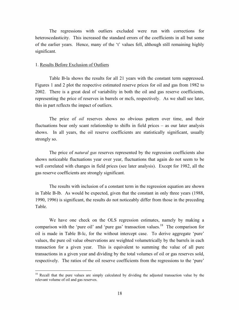
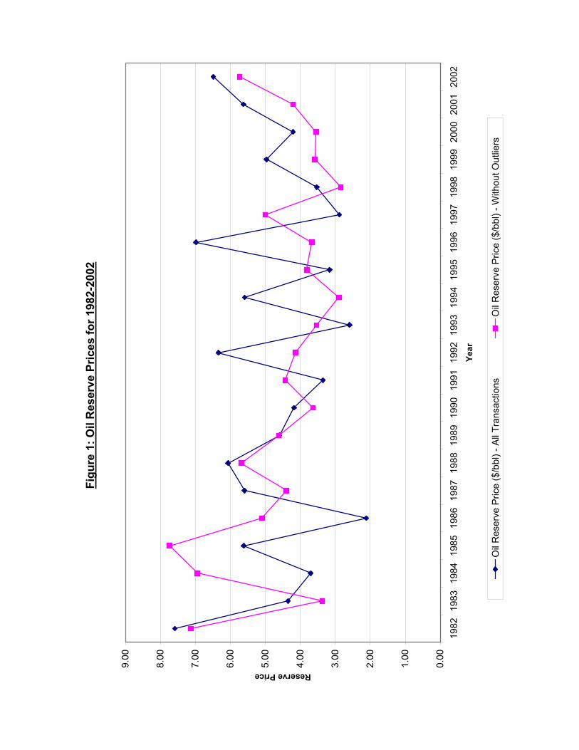
Table B-la shows the results for all 21 years with the constant term suppressed. Figures 1 and 2 plot the respective estimated reserve prices for oil and gas from 1982 to 2002. There is a great deal of variability in both the oil and gas reserve coefficients, representing the price of reserves in barrels or mcfs, respectively. As we shall see later, this in part reflects the impact of outliers.
The price of oil reserves shows no obvious pattern over time, and their fluctuations bear only scant relationship to shifts in field prices – as our later analysis shows. In all years, the oil reserve coefficients are statistically significant, usually strongly so.
The price of natural gas reserves represented by the regression coefficients also shows noticeable fluctuations year over year, fluctuations that again do not seem to be well correlated with changes in field prices (see later analysis). Except for 1982, all the gas reserve coefficients are strongly significant.
The results with inclusion of a constant term in the regression equation are shown in Table B-lb. As would be expected, given that the constant in only three years (1988, 1990, 1996) is significant, the results do not noticeably differ from those in the preceding Table.
We have one check on the OLS regression estimates, namely by making a
comparison with the ‘pure oil’ and ‘pure gas’ transaction values.18 The comparison for oil is made in Table B-lc, for the without intercept case. To derive aggregate ‘pure’ values, the pure oil value observations are weighted volumetrically by the barrels in each transaction for a given year. This is equivalent to summing the value of all pure transactions in a given year and dividing by the total volumes of oil or gas reserves sold, respectively. The ratios of the oil reserve coefficients from the regressions to the ‘pure’
18 Recall that the pure values are simply calculated by dividing the adjusted transaction value by the relevant volume of oil and gas reserves.
19
oil unit values differ markedly. There is no consistency, except that the regression coefficients are lower than the ‘pure’ oil transactions in about half the sample. Only in eight of the 21 years (1982, 1987, 1988, 1989, 1990, 1995, 1998, 2000) are the ratios within 10 percent of unity.19
Comparisons for natural gas are shown in Table B-ld. Again there is a large spread in the ratios of the regression values to the ‘pure’ values. And yet again in only eight years – 1986, 1987, 1989, 1998 through 2002 – were the ratios within 10 percent of unity. In contrast to oil, in the majority of years the regression coefficients exceeded the ‘pure’ values.
We conclude that the reserve values derived from the overall sample of transactions differ markedly in most years from the pure transaction sample. However, in many years the number of ‘pure’ observations is small, contributing to variability between the two sets of reserve values. 2. Results Excluding Outliers
The next set of Tables in Appendix B looks at what happens when we exclude the outliers. With the exception of 1985 and 2000, all the oil reserve coefficients are strongly significant (see Table B-2a, without constant). Their amplitude of variation, while large, is less than when the outliers are included, as would be expected. Much the same comment applies to the natural gas reserve coefficients, and no statistically insignificant values were recorded except for 1982. Overall, the gas coefficients were more stable over time than those for oil.
Results with an intercept are shown in Table B2-b, and show a similar pattern to those without it. The constant term was significant in seven years (1983, 1984, 1985, 1987, 1998, 2000, and 2001).
The oil coefficients are plotted in Figure 1; those for gas are plotted in Figure 2. The plots are shown both with and without outliers, for the without intercept case.
19 These results are notwithstanding the fact that regression data include the ‘pure’ oil cases (see earlier).
Figu
re 1
: Oil
Res
erve
Pric
es fo
r 198
2-20
02
0.00
1.00
2.00
3.00
4.00
5.00
6.00
7.00
8.00
9.00
1982
1983
1984
1985
1986
1987
1988
1989
1990
1991
1992
1993
1994
1995
1996
1997
1998
1999
2000
2001
2002
Year
Reserve Price
Oil
Res
erve
Pric
e ($
/bbl
) - A
ll Tr
ansa
ctio
nsO
il R
eser
ve P
rice
($/b
bl) -
With
out O
utlie
rs
Figu
re 2
: Nat
ural
Gas
Res
erve
Pric
es fo
r 198
2-20
02
0.00
0.20
0.40
0.60
0.80
1.00
1.20
1.40
1.60
1.80
1982
1983
1984
1985
1986
1987
1988
1989
1990
1991
1992
1993
1994
1995
1996
1997
1998
1999
2000
2001
2002
Year
Reserve Price
Nat
ural
Gas
Res
erve
Pric
e ($
/mcf
) - A
ll Tr
ansa
ctio
nsN
atur
al G
as R
eser
ve P
rice
($/m
cf) -
With
out O
utlie
rs
22
The next Table (B-2c) focuses specifically on the impact of the constant on the regression coefficients. For oil, only in three years (1982, 1998 and 2000) did the constant affect the regression coefficient by more than 10 percent. For natural gas, only in 1982 and 1985 did the impact of the constant on reserve values exceed 10 percent.
Table B-2d summarizes the impact of the exclusion of outliers on the reserve coefficients. The ratio of the oil and gas regression coefficients with and without the outliers is calculated in the no constant case. The impact of suppressing the outliers is considerable. And this holds in the case of both oil and gas (also see Figures 1 and 2).
Another approach to the issue of unusual observations is to apply robust regression techniques.20 As an example, ‘M Class’ estimators and ‘Least Trimmed Square’ estimators were calculated for our total set of observations for the year 1996. The results both confirmed the presence of unusual, influential observations and yielded estimated coefficients similar to ours after we excluded outliers. While this analysis was only confined to one year, it suggests our ‘ad hoc’ rules for identifying outliers, described in Section II, are broadly congruent with those from a robust regression approach.
Table B-2e compares the oil regression values (no constant) with the weighted pure oil case values (outliers excluded in both instances). No clear pattern over time emerges. This is quite similar to the earlier corresponding comparison before adjustment for outliers, although the number of years when the ratio is within 10 percent of unity is 11, compared with eight years for all transactions (see Table B-1c). Much the same conclusion applies to natural gas. There was a considerably closer correspondence between the natural gas regression coefficient values and the ‘pure’ transaction values when the outliers were excluded. The amplitude of variation, while noticeable, is less than when outliers are included in the sample (Table B-2f). However, the number of years when the ratio is within 10 percent of unity remains at eight, the same as for the all transaction case (Table B-1d). 3. Influence of Reserves Status
Information was available for certain transactions that distinguished between those where reserves were on production and those where they were partly fallow. In the latter case the properties may include prospective reserves normally classified as proved
20 We are grateful to Adonis Yatchew, University of Toronto, for this suggestion.

23
undeveloped, developed but not on production, probable or possible. Other things equal, the in situ reserve values for reserves on production would be expected to exceed those for dormant reserves. The theoretical margin between two identical properties, one on production, the other not developed, would be the development cost per unit of reserve, in the absence of any option value for the undeveloped reserve. We tested the proposition of such differential values using our database of 1456 mixed transactions, of which 981 observations related to properties not on production.21 We caution that the reason why so many observations are in this category may be lack of production information: that is, the numbers may well be exaggerated.
Specifically, we performed the following regression: adjprice = [a1
o + a2oDo]Ro + [a1
g + a2gDg]Rg
where: adjprice is the transaction price (after elimination of non reserve assets)
the ‘o’ superscript denotes oil the ‘g’ superscript denotes gas a1 and a2 are the two coefficients for each reserve being tested
R denotes reserves sold D denotes a dummy variable for reserves on production.
A priori, we expect both the a1 and a2 coefficients to be positive: reserves already producing would be expected to be worth more than those lying fallow. The results are shown in Table C-2 (excluding outliers, no constant). For oil, the first coefficient is positive as expected (except for 1985). However, eleven of the second coefficients are negative, although only two of these are statistically significant. Of the nine positive second coefficient values, four are significant. For natural gas, all the first coefficients are positive, but 12 second coefficients are negative, of which five are statistically significant; only two of the positive coefficients are significant. We treat these findings as broadly confirming that the sales value of oil reserves on production exceeds that where developed properties are either not producing, or are
21 This set includes observations where oil reserves are not on production, observations where gas reserves are not on production, and where both are dormant.
24
only partly on production. The results for natural gas are murky. 4. Influence of the R/P Ratio
A factor which can be expected to influence reserve values is the rate at which reserves are produced. Evidence for such an effect is likely confined to cross section data. The shift in time series data for R/P ratios is too gradual to reveal impacts.
US (remaining) reserve to production ratios are shown for oil and gas in Table C-1, Appendix C. Those for oil are quite stable; those for gas show some tendency to fall.
The years during which we had an appreciable number of transactions containing R/P ratio information was confined to 1989, 1990 and 1992 to 2002, inclusive. To test whether the R/P ratio affects the transaction price we performed the following regression:
adjprice = [a1o + a2
oHo]Ro + [a1g + a2
gHg]Rg where: adjprice is the transaction price (after elimination of non reserve assets)
the ‘o’ superscript denotes oil the ‘g’ superscript denotes gas a1 and a2 are the two coefficients for each reserve being tested
R denotes reserves sold H denotes the R/P ratio.
The regression was run without a constant term.
The greater the R/P ratio, the lower the rate of production. The lower the rate of production, the lower the expected price of reserves, other things equal. Hence the expected sign of the a2 coefficient attaching to the H variable (the R/P ratio) would be negative.
In the case of oil the a2 coefficient is negative in 10 of the 13 years for which we had data; it was significant in four of the 10 cases. In these years, the coefficient shows a great degree of variation, from -$1.64/bbl in 1989 to -$0.01/bbl in 1996. In all three years in which the coefficient was positive, it was insignificant.
25
In the case of gas, a2 is negative in all years but one (and here it was insignificant). And of the 12 years in which it is negative, it was significant in eight instances. The absolute value of the incremental coefficient is less than 10 cents/mcf in all years except 2001.
Our broad conclusion is that the transaction data do support the proposition that reserve prices would be inversely related to R/P ratios – and especially so for natural gas.
In summary: the impact on reserve prices of the two types or transactions discussed above – of whether production is taking place and of the rate of production – has the following implication. Unless the mix of transactions by these categories was reasonably constant, some of the variation in estimates of reserve prices among years will reflect compositional shifts in transaction types. Hence caution has to be exercised in any interpretation of temporal trends in estimated reserve prices. This seems to apply to a greater degree to natural gas than to oil reserve prices.22 5. Relationship Between Reserve Regression Coefficients and Field Prices
Expected field prices are an important determinant of reserve values, values that are influenced by current and previous field prices. We made some simple tests to see whether the annual estimates of oil and gas reserve prices calculated from the regressions displayed any obvious relationship with current and lagged field prices. We confined the tests to a simple linear regression of in-ground reserve prices, represented by our estimated oil and gas regression coefficients on field prices. We note that since reserve prices are influenced by field price expectations it is by no means clear in theory that a zero current or lagged field price would indicate zero reserve prices. Hence reserve prices could be positive even if field prices were zero. There is, then, a preference for including a constant term in the equation specification. The price series used are shown in Table C-4.
The regression results for both oil and natural gas are shown in the upper panel of Table C-5 for the two sets of regressions where the reserve price was regressed on each of contemporary field prices, prices lagged one year, and prices lagged two years. For all oil and gas equations the intercept is positive and significant. Oil reserve prices are positively (and significantly) related to field prices, whether contemporary or lagged one
22 Our 1996 paper included some analysis of location (regions) reserve values. Change in regional mixes of transactions is another source of variation.
26
or two years; the results suggest about 12 to 15 percent of any increase in field prices would be reflected in reserve prices. But the degree of linear fit of the three oil equations is modest. Gas reserve prices are also positively related to field prices, but all coefficients are statistically insignificant; moreover, the degree of linear fit is trivial. We also subjected the time series of reserve and field prices to stationarity tests. Stationarity was not rejected for the series of reserve prices, but was rejected for the field price series. Stationarity was not rejected for the residual terms of the equation results shown in the upper panel of Table C-5; nor was it rejected for the first differences of the respective series in field prices. Thus the regressions are of I(0) variables on I(1) variables and result in I(0) residual terms. The stationarity tests used a 5 percent level of significance throughout.
The fact that field prices were found to be I(1) while reserve prices were I(0) encouraged regressing reserve prices on the first differences field prices, since both variables then would be I(0). The results are shown in the lower panel of Table C-5. A fit is absent and coefficients for field price differences are insignificant, except for natural gas with a one period lag in field price first differences.23 The constant term roughly picks up the average values of the respective reserve prices, which is consistent with what one anticipate for expected reserve prices when field prices are constant (first differences are zero). Overall, we find first differences in field prices do not have a material impact on reserve prices. 6. Reserve Prices and Company Performance Differences between the actual expenditures incurred by a company and those implicit using the in situ prices generated from industry wide data will indicate the extent to which a company over or under performed in relation to the market. For example, suppose in year 2002 a company spent $500 million in acquiring 100 million barrels of oil and 100 billion cubic feet of natural gas. In situ prices for that year are $5.74 per barrel and $0.88 per mcf (see Table B-2a). At these prices, the estimated market value of the company’s transaction would be $574 million for the oil and $88 million for the gas, a total of $662 million. In this example the company seemingly would have outperformed the market to the tune of $162 million, or about 32 percent.
23 The sign of the coefficient is ambiguous. For example, a positive price change might indicate a peak, depressing price expectations embedded in reserve values, resulting in a negative coefficient; or it might indicate further price increases on the way, resulting in a positive coefficient.
27
The in situ prices are subject to uncertainty. Two standard deviations either side of the point estimates cited above yield a spread in values for oil of $4.58 to $6.80 per barrel, for gas $0.70 to $1.06 per mcf.24 At the lower price bounds the imputed value of the transaction would be $528 million, and the company would still have outperformed the market by $28 million, or some 5 percent. At the upper bound, the corresponding figures would be $786 million, $286 million and 57 percent.
24 For standard errors of the coefficients, see Table B-2a.
28
IV. Reserve Prices, Hotelling Values, Price Expectations and Returns to Holding
The Hotelling Valuation Principle states that the market value of a mineral in the ground at any point in time is equal to the prevailing net price per unit of production (Miller and Upton [1985]). In the first part of this section we relate the estimates of reserve prices discussed in Section III to estimates of Hotelling Values. We then examine what price expectations for oil and gas respectively may underlie our estimates of reserve prices. Finally, we look at one period returns to holding reserves in the ground, in the Hotelling context. 1. Reserve Prices and Hotelling Values - A Comparison
Hotelling Values are the net price, which we write as: p-c
where: p is present price of oil or gas as produced at the field (wellhead) c is unit extraction cost, plus non-cost outlays (non-income taxes, royalties).
The assumption here is that title to the reserve in the transaction passes at the field
gate, and that the field is already developed. To the extent the transaction includes undeveloped reserves, the value of ‘c’ would need adjustment to add relevant development cost. The Hotelling Value, accordingly, would be smaller. However, results in our 1996 paper and in Section III of this paper indicate that transactions with some undeveloped reserves – reserves not on production – were not necessarily of lower value than those for just developed reserves, which obscures the picture. We estimate national averages for the p-c values for the period 1982-2002. The oil and gas field prices (p) used are those shown in Table C-l, Appendix C. Operating costs (c) essentially consist of three components: a fixed element; one that varies with output; and royalties and taxes that are field price sensitive. A suitable historical series of operating costs was not available. Instead, reliance was placed on evidence that over a period of time when data were available on unit operating costs they approximated 35 percent of gross field values (Adelman [1992, Table 2]). The procedure we adopt of estimating operating costs as 35 percent of field prices treats them as ad valorem, whereas we know only a portion of them behave in this manner. Nevertheless, it remains the best approximation at hand. To the extent that operating costs are underestimated in a given year, estimated Hotelling Values would be inflated, and vice versa.
29
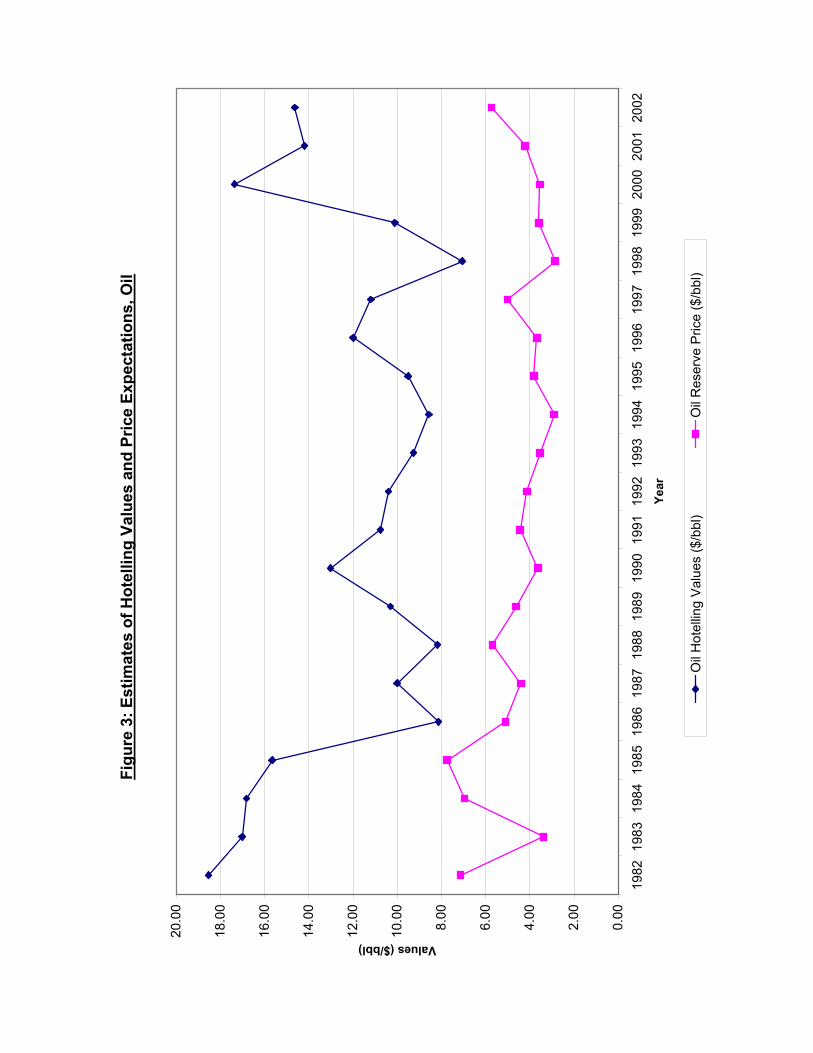
The annual Hotelling Values (HV) so estimated are shown in Tables D-1 through D-4 under the column headed “Net Field Price” (column 9). These Tables relate respectively to the oil values from all transactions, ‘pure’ oil values, natural gas values from all transactions, and ‘pure’ natural gas values. a) Oil Results
The HVs for oil are graphed in Figure 3 for 1982 to 2002, along with the reserve prices estimated from the regressions in Table B-2a (excluding outliers, no intercept), Appendix B. Figure 3 shows that in all years the Hotelling Values comfortably and in most instances considerably exceed corresponding reserve prices. How significant is the spread between them?
The standard errors of the reserve prices are given by the regression results and reproduced in column 5 of Table D-1. This enables us to calculate by how many standard deviations the HVs are away from the reserve prices. The results are shown in Column 11. If we assume the estimated reserve price is Normally distributed within each year, as the Central Limit theorem would suggest, then 1.96 standard deviations would bracket 95 percent of them. It follows that the results in column 11 decisively reject the null hypothesis that the recorded differences between the HVs and reserve prices are not statistically significant. In only one year (1985) is the HV spread below 1.96.
The same analysis as undertaken for the oil values from the regression equation is pursued for the ‘pure’ oil reserve prices and is shown in Table D-2. In all years bar 1986 (the year of the OPEC price crash) the HVs exceed the reserve prices. And the null hypothesis that the differences are not statistically significant is rejected in all years except 1986, 1988 and 1994. b) Natural Gas Results
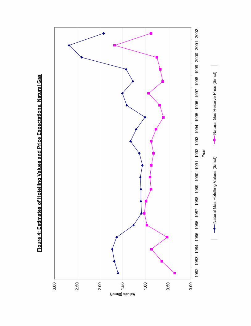
The HVs for natural gas national averages are listed in Table D-3, Appendix D, in relation to reserve prices and displayed in Figure 4. In all years except two (1987, 1989) the HVs exceed the reserve prices by a statistically significant margin.
Figu
re 3
: Est
imat
es o
f Hot
ellin
g Va
lues
and
Pric
e Ex
pect
atio
ns, O
il
0.00
2.00
4.00
6.00
8.00
10.0
0
12.0
0
14.0
0
16.0
0
18.0
0
20.0
0
1982
1983
1984
1985
1986
1987
1988
1989
1990
1991
1992
1993
1994
1995
1996
1997
1998
1999
2000
2001
2002
Year
Values ($/bbl)
Oil
Hot
ellin
g V
alue
s ($
/bbl
)O
il R
eser
ve P
rice
($/b
bl)
Figu
re 4
: Est
imat
es o
f Hot
ellin
g Va
lues
and
Pric
e Ex
pect
atio
ns, N
atur
al G
as
0.00
0.50
1.00
1.50
2.00
2.50
3.00
1982
1983
1984
1985
1986
1987
1988
1989
1990
1991
1992
1993
1994
1995
1996
1997
1998
1999
2000
2001
2002
Year
Values ($/mcf)
Nat
ural
Gas
Hot
ellin
g V
alue
s ($
/mcf
)N
atur
al G
as R
eser
ve P
rice
($/m
cf)
32
With the exception of one year (1989) the ‘pure’ gas results (see Table D-4) show the HVs as exceeding the reserve values but the margins are statistically insignificant in ten years. This result mainly reflects the higher standard errors for ‘pure’ gas transactions compared with the regression coefficients. 2. Oil and Gas Price Expectations
Given information on field prices, production to reserve ratios and the discount rate it is possible to estimate the implicit growth rate in field prices that would be consistent with a given reserve price (Adelman and Watkins [1995, p.669]). Predicated on certain simplifying assumptions, the general expression for the growth rate in prices implicit in the reserve prices is given by: g = i + a{1- [(p-c)/V]} (6) where g = annual growth rate in prices
i = discount rate a = production / reserve ratio p = field price c = extraction cost V = reserve price.
For oil we need data on ao, po, co, Vo; and for gas, ag, pg, cg, Vg. In the case of
both ao and ag (the production to reserves ratio), we make a refinement to correct for shorter than infinite reservoir life, and write ‘a’ in general terms as: a = (P/R) - (P/R)2 where P/R = production to reserve ratio.25
The values for field prices, p, are taken from the earlier tables (Table C-4); the P/R ratios are of course the inverse of the R/P ratios in Table C-1. The industry discount rate adopted was a nominal rate of twice the long-term bond rate (LTBR), as an approximation to a suitable rate of return on capital. This accommodates an assumed risk
25 When production life is infinite, a = P/R; see Section I.
33
premium equivalent to the LTBR. The LTBR itself has a range from about 13.0 percent in 1982 to 4.6 percent in 2002.26
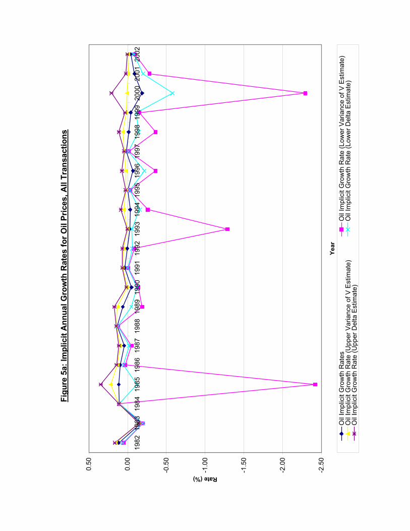
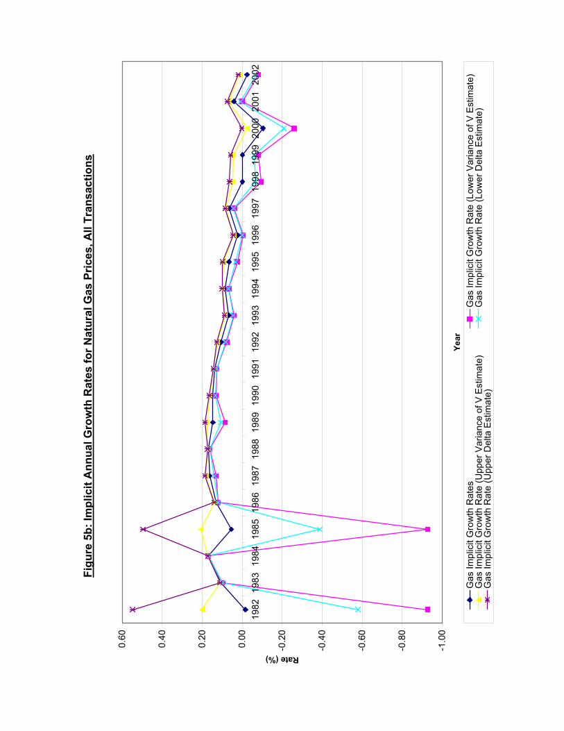
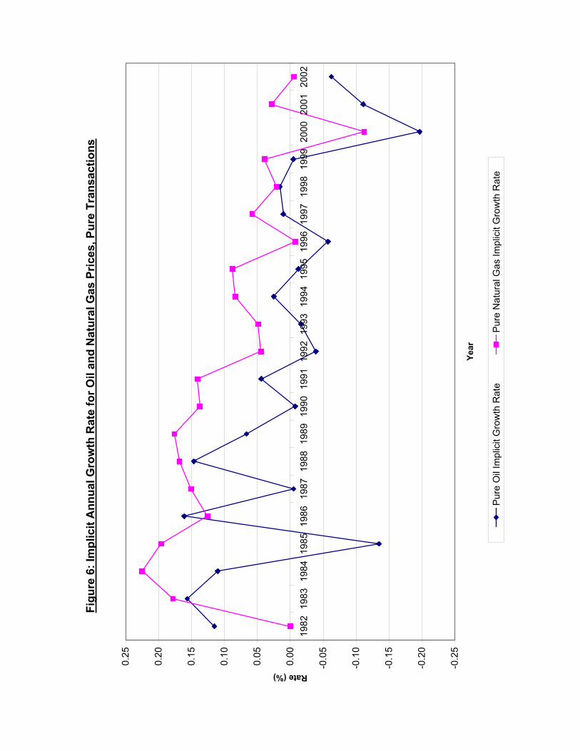
The estimated implicit growth rates of field prices embedded in estimates of the value of reserves, V, are listed in column 8 in Tables D-l through D-4 for reserve prices derived from the regression without an intercept, after exclusion of outliers. The results are illustrated in Figure 5a (oil, all transactions), Figure 5b (natural gas, all transactions) and Figure 6 (just the ‘pure’ transactions).
Striking differences are revealed between oil and gas price expectations. Those for oil mirror perceived conditions in the world oil market. We suggest that the expectation of declining prices for the four years 1982-1985 reflect the weakening market after the price peak of 1981. Expectations of rising prices, 1986 to 1989, reflect anticipated recovery from the price nadir of 1986. Resumption of expected declines in prices, 1990 to 1997, express concern about OPEC discipline, concerns that seemed to end in 1998 and 1999. Anticipated declines in 2000, 2001 and 2002 reflect a supposition of continuing weakness on the OPEC front, in relation to prevailing prices. These trends in expectations also hold in much the same way for the ‘pure’ oil reserve values (see Table D-2, column 8).
In contrast to oil, price expectations for natural gas are persistently positive, with the main exception of year 2000 (year 2002 is also negative, but the estimated value is a trivial 1 percent). The anticipated sharp decline in gas prices for year 2000 probably reflects the peak price recorded at that time. The ‘pure’ gas results show much the same pattern as for all transactions (see Table D-4).
This pattern of variation between oil and gas price expectations is consistent with our knowledge of industry assessments and forecasts.
26Federal Reserve Board: Ten Year Treasury Rate. (http://www.federalreserve.gov/releases/h15/data/a/tcm10y.txt).
Figu
re 5
a: Im
plic
it A
nnua
l Gro
wth
Rat
es fo
r Oil
Pric
es, A
ll Tr
ansa
ctio
ns
-2.5
0
-2.0
0
-1.5
0
-1.0
0
-0.5
0
0.00
0.50
1982
1983
1984
1985
1986
1987
1988
1989
1990
1991
1992
1993
1994
1995
1996
1997
1998
1999
2000
2001
2002
Year
Rate (%)
Oil
Impl
icit
Gro
wth
Rat
esO
il Im
plic
it G
row
th R
ate
(Low
er V
aria
nce
of V
Est
imat
e)O
il Im
plic
it G
row
th R
ate
(Upp
er V
aria
nce
of V
Est
imat
e)O
il Im
plic
it G
row
th R
ate
(Low
er D
elta
Est
imat
e)O
il Im
plic
it G
row
th R
ate
(Upp
er D
elta
Est
imat
e)
Figu
re 5
b: Im
plic
it A
nnua
l Gro
wth
Rat
es fo
r Nat
ural
Gas
Pric
es, A
ll Tr
ansa
ctio
ns
-1.0
0
-0.8
0
-0.6
0
-0.4
0
-0.2
0
0.00
0.20
0.40
0.60
1982
1983
1984
1985
1986
1987
1988
1989
1990
1991
1992
1993
1994
1995
1996
1997
1998
1999
2000
2001
2002
Year
Rate (%)
Gas
Impl
icit
Gro
wth
Rat
esG
as Im
plic
it G
row
th R
ate
(Low
er V
aria
nce
of V
Est
imat
e)G
as Im
plic
it G
row
th R
ate
(Upp
er V
aria
nce
of V
Est
imat
e)G
as Im
plic
it G
row
th R
ate
(Low
er D
elta
Est
imat
e)G
as Im
plic
it G
row
th R
ate
(Upp
er D
elta
Est
imat
e)
Figu
re 6
: Im
plic
it A
nnua
l Gro
wth
Rat
e fo
r Oil
and
Nat
ural
Gas
Pric
es, P
ure
Tran
sact
ions
-0.2
5
-0.2
0
-0.1
5
-0.1
0
-0.0
5
0.00
0.05
0.10
0.15
0.20
0.25
1982
1983
1984
1985
1986
1987
1988
1989
1990
1991
1992
1993
1994
1995
1996
1997
1998
1999
2000
2001
2002
Year
Rate (%)
Pur
e O
il Im
plic
it G
row
th R
ate
Pur
e N
atur
al G
as Im
plic
it G
row
th R
ate
37
3. Confidence Limits for Price Expectations What sort of confidence interval might bracket these estimates of implicit growth rates (g)? Sensitivities could be established by using different values for the exogenous variables i, a, p and c. However, we prefer to focus on the statistical variability in V, the reserve price, since we do have an estimate of its variance from the regression analysis. If we assume V does not co-vary with the exogenous variables, upper and lower bounds for g can be calculated numerically as a function of the variance of V. In the 1996 paper, we took the two standard error spread either side of V and found the corresponding values of g from our formula, conditional on assumed values for i, a, p, and c. We assumed this spread represented the 95 percent confidence interval – (see Adelman and Watkins [1996, p28]), which is reasonable if we interpret g as a mean value, with an associated Normal distribution.
An alternative approach is a Monte Carlo simulation. But there are two problems here. First, we would have to assume all the variables were independent, a questionable assumption – for example consider V and i. Second, we have little information on what kind of distributions might reasonably characterize the relevant variables. Another approach, one implicit in what we did in 1996, is to argue that variability in p,c,i and a is already embraced by the variability of V, since V essentially is the present value of the expected stream of net revenues from production of the reserve over time. That is, the variability in the components of V contributes to the variability in V itself. The implication is that we can simply look at the variability in V, and treat the other variables on the formula as constant. Hence we could write g as:
g = b - d/V (7)
where b = i + a d = a(p – c).
It is tempting to conclude that the variability in V embraces all the variability in
its components. However, this is not so. It includes that part of the variability in p, c, a, or i correlated with V. It doesn’t include all their inherent variability. The restriction, however, is not damaging because our formula for g is after all derived from the
38
assumption that V is predicated on net present values incorporating p, c, a, and i. Nevertheless, it remains a conditional variance. As already mentioned, the central limit theorem (CLT) suggests V is normally distributed. Thus there is no limit on the tails of the distribution of V: some of the probability distribution of V will be negative. However, V is essentially positive. Moreover, we have the inverse of the Normal distribution and values of V that are zero would be inadmissible, since they would yield values for g of infinity. In short, we have a restricted domain issue. Also note that quite apart from the sign of V issue, the spread of g values predicted on the confidence limits of V will not be symmetric. An approach that offers some relief is to employ the ‘delta’ method.27 Here, if we designate the number of observations on which V for a given year is based as n, then it can be shown that, in relation to equation (7), the expression √n(b + d/V – (b + d/V)) is approximately distributed Normally with mean zero and standard error of (d/V2)σV where V is the estimated value of V and σV is its standard error. Using this approach we multiply the standard error of V given by column 5 of our ‘D’ tables by the product of ‘d’ divided by V2 to estimate the standard error (se) of g. The approximate 95 percent confidence interval would be given by the estimated value of g plus and minus two times its standard error calculated as above. If we interpret this as an approximation to the confidence interval for the mean of g, then again the CLT suggests a (symmetric) Normal distribution.
We use both approaches below: our 1996 method predicated on the standard errors of V, and the ‘delta’ method. Both approximations make a statement about the probability of the mean of g, not about the probability distribution of expected prices. That distribution may not be symmetric at all.
Upper and lower bounds for the implicit growth rates resulting from inserting in equation (6) values of plus and minus two standard errors from the estimated V and those resulting from the delta method are shown in Tables D-5 and D-6 respectively for oil and natural gas.28 The intervals are also shown in Figures 5a and 5b (for all transactions). 27 We are indebted to Adonis Yatchew, University of Toronto, for this suggestion; also see W.Greene Econometric Analysis, Third Edition, 1997, p124. 28 In the variance of V method, a floor boundary value for V was imposed of 55 cents per barrel and 10 cents per mcf.
39
a) Variance of V Method
As mentioned earlier, the implicit confidence intervals for g are not symmetric. Indeed the degree of asymmetry is noticeable: the upper confidence interval being much tighter than the lower level, with the spread from the mean usually in single digits, in terms of percentage points. And there is considerable variability among years.
In marked contrast to oil, the confidence intervals for natural gas are generally tight, at 1 to 2 percentage points, and with quite modest variability among years. This result reinforces our conclusion that price expectation behavior between oil and gas is quite different. b) Delta Method
The spreads between the lower and upper limits are tighter than for the other method, and are symmetric. For oil, the four standard error spreads (difference between lower and upper bounds) vary between close to zero and a peak of 79 percentage points, but in most years the spread is less than 20 percentage points. The results for natural gas confirm the finding under the variance method of much tighter and consistent confidence intervals than for oil; in the great majority of years (16 out of 21), the four standard deviation spread is in the single digit range (percentage points).
It is also possible that the estimates of implicit growth rates in prices include expected cost reductions. But such technological and other improvements are more manifest at the exploration and development stage than at the production stage.
Expression (6) is derived on the assumption that the reserve price is a straightforward function of future net cash flows. Insofar as V includes an option value, the estimates of g, the implicit growth rate, are overstated. We are unable to measure the extent of any such bias. As long as it applies equally to oil and gas reserve values our finding of noticeable differences between oil and gas price expectations remains. We also note that option values are more important for undeveloped than for developed reserves already on production.
40
4. Mineral Holding Values A corollary of the Hotelling Principle is that in-ground prices increase, one period over another, at the industry’s discount rate. In Table D-7 we compare each year’s value of a unit in-ground with the previous year’s. The reserve prices in columns 3 and 6 are the regression values in Tables D-1 and D-3. The percentage increase or decrease in columns 4 and 7 measures the return to holding the reserve in the ground an additional year, rather than selling it at the year’s price.29 We subtract from that return the one-year risk-free discount rate, approximated by the one-year US Treasury bill rate, a rate which also reflects expected inflation. The apparent achieved rate premia for oil (column 5) and for gas (column 8) are therefore free of any distortion caused by the time value of money and by expected inflation, and are plotted in Figure 7.
For oil, in 12 out of the 20 years the achieved risk premia are negative, and indeed the mean achieved risk premium is a negative 1.7 percent, to boot. However, there is also a wide dispersion around the mean: its standard error is 8 percentage points. For natural gas, the risk premia are negative in 11 out of 20 years; however, the mean achieved risk premium is positive, at 5.3 percent, but with a high standard error of 9.5 percentage points. These high standard errors of the mean achieved risk premia undermine any precision in statistical testing of hypotheses about them. Instead, we make the simple comparisons below.
Specifically, we compare the achieved risk premia with suitable minimum risk
premium for petroleum finding and development activities which the reserve assets represent. Earlier we approximated that risk premium as the LTBR.30 We term this the required risk premium, and list it in column 9, Table D-7. It has a mean of 7.5 percent and a standard error of 0.5 percent. In the case of oil, this mean compares with a mean achieved risk premium of -1.7 percent, and in only seven of the 20 years does the achieved premium exceed the required level. For natural gas, parallel comparisons show a mean required premium of 7.5 percent and mean achieved levels of 5.3 percent; in just six of the 20 years do achieved premia exceed required premia. Overall, these comparisons offer scant support for the HVP of in-ground values increasing one period over another at the industry’s discount rate.
29 For some results for oil, 1949-1986, see Adelman & Watkins [2003]. 30 See p32 above.
Figu
re 7
: Ret
urns
to H
oldi
ng O
il an
d N
atur
al G
as R
eser
ves
-0.8
00
-0.6
00
-0.4
00
-0.2
00
0.00
0
0.20
0
0.40
0
0.60
0
0.80
0
1.00
0
1.20
0
1983
1984
1985
1986
1987
1988
1989
1990
1991
1992
1993
1994
1995
1996
1997
1998
1999
2000
2001
2002
Year
Return (%)
Ach
ieve
d R
isk
Pre
miu
m fo
r Oil
Ach
ieve
d R
isk
Pre
miu
m fo
r Nat
ural
Gas
42
An operator can substitute for developing a barrel of oil in the USA, a barrel of oil anywhere in the world, and vice versa. (He cannot yet do this to develop natural gas.) Hence the data of Table D-7 permit a simulation, for the worldwide industry of exploration and development. Each year we borrow at the US (one year) riskless rate, to buy a reserve barrel of oil, at the year’s price for oil in the ground. We hold it for a year, and then sell at the next year’s price. In the 20 trials, we expect irregular fluctuation; such that we would win a few, lose a few. But if original oil in the ground worldwide were fixed, while its consumption continues and even grows, it must shrink over time. Correspondingly, the unit value of what remains in the ground must increase over time. Moreover, given the Hotelling corollary one would expect to earn enough to more than offset the year-to-year risks. But the table shows that even before considering any risk, we lose close to 2 percent per year on average. Any risk allowance will make the losses worse. It is impossible to reconcile these data for the last 20 years with the belief in a fixed stock, nor in worldwide growing scarcity. But we do not extrapolate and argue that because oil and gas have not become more meager in the past 20 years, supply must always be plentiful. That is more than anyone can know.
43
V. Value of US Oil and Gas Reserves Our estimates of reserve prices discussed in Section III can be applied to value US crude oil reserves in recent years. The results are shown in the following Table 1. The private values in the table should be multiplied by some 1.3 to approximate the social values (see below).
Table 1 Estimated Market Values of U.S. Oil and Natural Gas Reserves
1999 2000 2001 End-of-year proved reserves Crude oil (B barrels) 21.8 22 22.4 Natural gas (T cu ft) 167.4 177.4 183.5 Market value per unit in situ Crude oil ($/barrel) 3.59 3.55 4.21 Natural gas ($/mcf) 0.67 0.75 1.68 Total market value ($ B) Crude oil 78.2 78.1 94.3 Natural gas 112.8 132.7 307.7 Total 191.0 210.9 402.0
2000 wealth
change 2001 wealth
change ($ B) ($ B) Value differences over previous year Crude oil ----- -0.1 +16.2 Natural gas ----- +19.9 +175.0 Weighted: 1999 prices Crude oil ----- +0.7 +1.4 Natural gas ----- +6.7 +4.1 Weighted: 2000 prices Crude oil ----- +0.7 +1.4 Natural gas ----- +7.5 +4.6 Weighted: 2001 prices Crude oil ----- +0.8 +1.7 Natural gas ----- +16.8 +10.2 The total value in current dollars of developed oil and gas reserves is in the neighborhood of $400 [$520] billion (bracketed figures are social values). Reserve quantities are from EIA publications; in situ values are from Table B-2a, Appendix B; weighted changes apply prices to reserve changes.
44
a) Excess of Social Over Private Values There is a downward bias in our estimates. They show the value of the reserve to the private owner, which mainly depends on the price expected to be received, net of expected expenses. As mentioned earlier, the total of these expenses has long been quite constant around 0.35 of the gross field price. Operating costs and royalties payable to land owners (public and private) are each about 0.15 of the price. The 0.05 remainder is non-income taxes. The royalties are not costs but transfer payments, a share of profits. If we assume that half of the taxes are payment for services (police and fire protection, etc.), then about 0.175 of the gross field price is a transfer payment. Hence the true social value of the reserve is probably about 1.27 times, i.e. (0.650+0.175)/0.650, the private value which we record.
Our detailed calculations in Table 1 were aimed at calculating private values. For purposes of national income accounting, we need to add 27 percent. Note here we assume that the field price to cost ratios would hold equally for the in situ values of reserves. b) U.S. Government Holdings We can also calculate the approximate value of the U.S. Government interest. Current oil and gas production on Federal offshore and onshore lands is roughly one-fourth of the national totals (API, Basic Petroleum Data Book, vol. 23, no. 1, (February 2003, tables IV-6 and XI-18). The Federal Government receives as royalty 0.155 of the gross field price for production from its lands. As noted above, the net to the owner has long been around 0.65 of the field price. Therefore the Federal interest per barrel is 0.155/0.65 = 0.2385 of the owners’ interest. The value to the private owners of all oil and gas reserves was estimated as $402 billion at the end of 2001. The U.S. Government had a share in one-fourth of the reserves, in which portion its interest was worth 0.2385 of an owner’s interest. Hence the total value of the Government’s oil and gas holdings was $402 x 0.25 x 0.2385 = $24 billion. However, this total makes no allowance for additional income in the form of bonus payments that the Government receives related to the properties from which production is extracted.
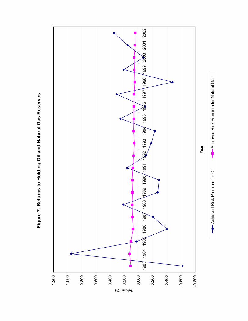
45
Typically such properties attract bonuses through auctions when reserves are at an undeveloped or prospective stage. And the amounts are sizeable. During 1954-2001, bonus payments for permission to drill and explore in Federal waters totaled $61.4 billion, compared with royalties of $67.8 billion. But the ratio has fluctuated enormously. In 1974, bonuses were 9.4 times royalties; in the latest year of available data, bonuses were only a tenth (0.10) of royalties (API, Basic Petroleum Data Book, vol. 23, no. 1, Tables IV-6, XI-10). These data do not suggest a convenient yardstick with which to adjust royalties to reflect additional income accruing to the US Government from bonus payments. The implication, nevertheless, is that our estimated value of the US Government oil and gas holdings is appreciably underestimated.
46
VI. Concluding Remarks
The results of this research paper are of interest in several ways.
Reserve value embraces (net) price forecasts over the life of the reserve. This is because it mainly reflects the net present value of all the production expected. The appraisal is made by a team of engineers, geologists, bankers, economists, and investors. Their forecasts may be wrong, but the values at which reserves change hands merit serious attention.
The difference between the value of existing reserves on production and the cost of finding and developing additional reserves is the governor of investment. The value: cost comparison is a clue to whether oil or gas reserve additions are expected to increase or decrease.
Oil and gas reserve values must be separately calculated. Barrels of “oil equivalent” is an artifact. Our research broadly confirms price and production data, and industry opinion: the oil and gas industries have been on a different track.
Oil reserve values show no visible trend, 1982-2002, sometimes falling, sometimes rising, as they have recently – but to levels in 2002 no higher than those in the mid-1980s. These movements reflect changing perceptions about the world oil market, not the US domestic market. Natural gas reserve prices tended to fall gradually, from 1984 to 1995, as deregulation became pervasive; since then there has been an erratic tendency to rise, indicating nascent tighter supply conditions. The Hotelling Valuation Principle (HVP) that the developed reserve value is equal to the field price net of extraction costs cannot be reconciled with the reserve values we have estimated. These show net prices averaging more than twice in-ground values, providing evidence more in favor of an old industry rule-of-thumb for reserve valuation, than for the HVP. The Hotelling theory, applied to actual data, does not support the notion of a fixed quantity of oil and gas “out there”. Indeed, experience of the last 20 years repudiates the idea of prescribed stock and associated inevitable scarcity. But there is no presumption of perpetual abundance. Oil and gas reserve values will register changing conditions. The national income needs to be adjusted for reserve accumulation or
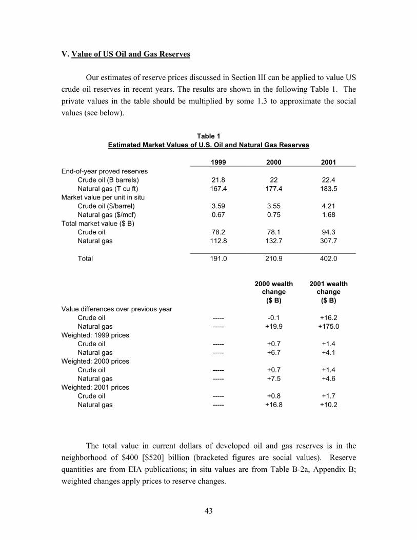
47
decumulation. Our measures are based on the premise that reserves are created and consumed like all other capital assets. There is little support for the theory that minerals are somehow unique, and that a unit produced today ineluctably means one less available in the future, except in a very elementary sense. Future reserves will be determined by future technology and costs on the one side, and future demands on the other.
Despite the defects in our estimates of income adjustments, they are more accurate than most other measures, which depend on arbitrary accounting rules to recapture original outlays over some assumed “service life.” Our estimates are based on estimated market values. The value of the (developed) mineral holdings of the U.S. Government is in the neighborhood of $24 billion.
We believe our estimates of reserve values could be improved in several ways. First, as always it would be nice to have more reserve transaction observations, and better information to “clean out” non-reserve assets more precisely. Second, there seems to be significant variation in reserve values according to reserve/production ratios, whether reserves are fallow, and so forth. Normalization for these variations would improve the consistency of estimates over time. Third, more data on operating costs would improve estimates of net prices, for comparison with in-ground values. Fourth, we need information on the extent to which reserve values might incorporate option values, ‘good will’ and the like. Fifth, estimation of unit development costs would enable us to infer finding costs by deduction of development costs from prices of developed reserves.
Measuring the capital costs of newly created reserves is a problem we have barely touched. Depending on the state of knowledge, they could be rising, falling, or stable. So far as we can discern, North American natural gas reserve prices and marginal costs have been relatively stable, at least until recently, while North American oil production has been gradually undermined by its rising costs in the face of quite stable worldwide costs.
Finally, we suggest that less attention be paid to the narrow stage of the Hotelling theatre. More effort should be devoted to estimating aggregate supply functions to see whether they are moving outward with new plays and technology overcoming depletion effects, or inward as depletion effects dominate, or whether there is a saw-off. Reserve prices are useful leading indicators of shifts in supply functions.
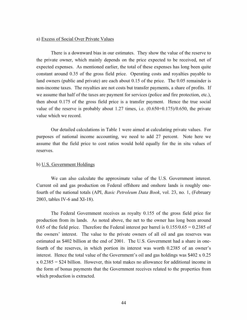
48
References [Adelman 1970] M.A. Adelman, “Economics of Exploration for Petroleum and Other
Minerals”, Geoexploration, vol. 8, pp. 131-150. [Adelman 1990] M.A. Adelman, “Mineral Production, with Special Reference to
Petroleum”, Review of Economics & Statistics, vol. 72, pp. 1-10. [Adelman 1992] M.A. Adelman, “OPEC at High Noon 1974-1981”, MIT Center for
Energy and Environmental Policy Research, 1992. [Adelman 1998] M.A. Adelman, “Crude Oil Supply Curves”, Proceedings of the IAEE
21st International Energy Conference (Quebec), 1998, pp. 1-6. [Adelman DeSilva & Koehn 1991] ---, Harindar DeSilva, and Michael F. Koehn, “User
Cost in Oil Production”, Resources & Energy v 13, pp 217-240. [Adelman & Watkins 1995] M.A. Adelman and G.C. Watkins, “Reserve Asset Values
and the Hotelling Valuation Principle: Further Evidence,” Southern Economic Journal, Vol 61, #3, Jan 1995.
[Adelman & Watkins 1996] M.A. Adelman and G.C. Watkins, “The Value of United
States Oil and Gas Reserves”, MIT- CEEPR 96-004 WP, May; an abbreviated version is in Advances in the Economics of Energy & Resources, vol 10, 1997, pp. 131-184.
[Adelman & Watkins 2003] M.A. Adelman and G.C. Watkins, “Resource Scarcity and
the Value of U.S. Oil and Gas Reserves”, Proceedings, IAEE 26th International Energy Conference, Prague, Czech Republic, June 2003.
[API 1983-1991] American Petroleum Institute, “Survey of Oil & Gas Expenditures,”
1983-1991 (annual). [Arrow 1987] Kenneth J. Arrow, “Hotelling”, in John Eatwell, Murray Milgate, and Peter
Newman, eds., A Dictionary of Economics (London: Macmillan) 1987, p. 67.
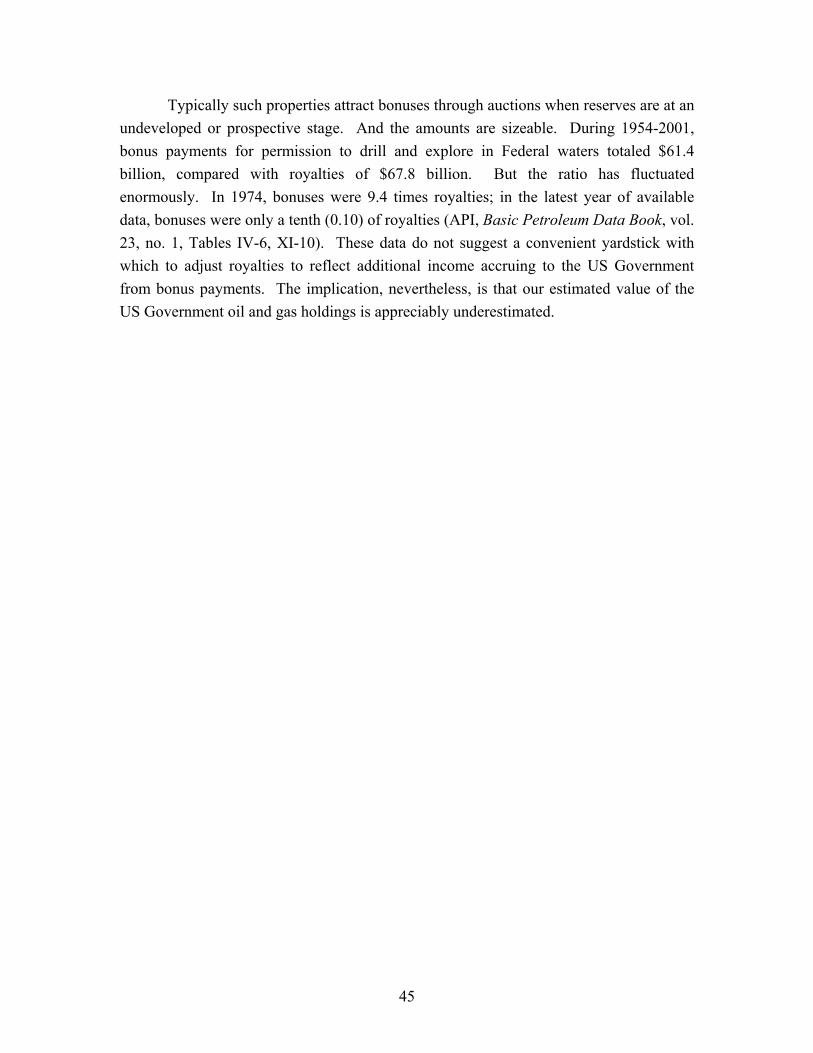
49
[Bradley 1987] Howard B. Bradley et al, Editors, Petroleum Engineering Handbook, Society of Petroleum Engineers, Richardson TX 1987, chapter 41 [incorporating Thomas C. Frick, Ed, Petroleum Production Handbook (McGraw Hill 1962)].
[Bradley & Watkins 1994] P.G. Bradley and G.C. Watkins, “Detecting Resource
Scarcity: the Case of Petroleum”, Proceedings of the IAEE 17th International Energy Conference, Stavanger, Norway, vol 2, 1994.
[Cairns and Davis 2001] Robert D. Cairns and Graham A. Davis “Adelman’s Rule and
the Petroleum Firm” The Energy Journal, vol 22, Number 3, pp 31-54. [Census ASOG 1973-1982] Bureau of the Census, “Annual Survey of Oil and Gas
Expenditures,” 1973-1982. [Census Bureau: Manufacturing & Mining] U.S. Bureau of Census, Manufacturing,
Mining, and Construction Statistics, “1997 Economic Census General Summary 1997: Mining”, p. 7.
[Chermak & Patrick 2002] J.M. Chermak and R.H. Patrick, “Comparing Tests of the
Theory of Exhaustible Resources”, Resource & Energy Economics, November, 301-326.
[Chernow 1998] Ron Chernow, Titan: the life of John D. Rockefeller (Random House)
1998. [DasGupta & Heal 1979] Partha DasGupta and G. M. Heal, Economic Theory and
Exhaustible Resources (Cambridge University Press). [EIA Reserves] EIA, “U.S. Crude Oil, Natural Gas, and Natural Gas Liquids Reserves,
2000 Annual Report,” December 2001, p.24. [Gately 1984] Dermot Gately, “OPEC: a Ten Year History”, Journal of Economic
Literature, vol 23, September, pp 1100-1114. [Gordon 1967] Richard L. Gordon, “A Reinterpretation of the Pure Theory of
Exhaustion”, Journal of Political Economy, vol. 75, pp. 274-286.
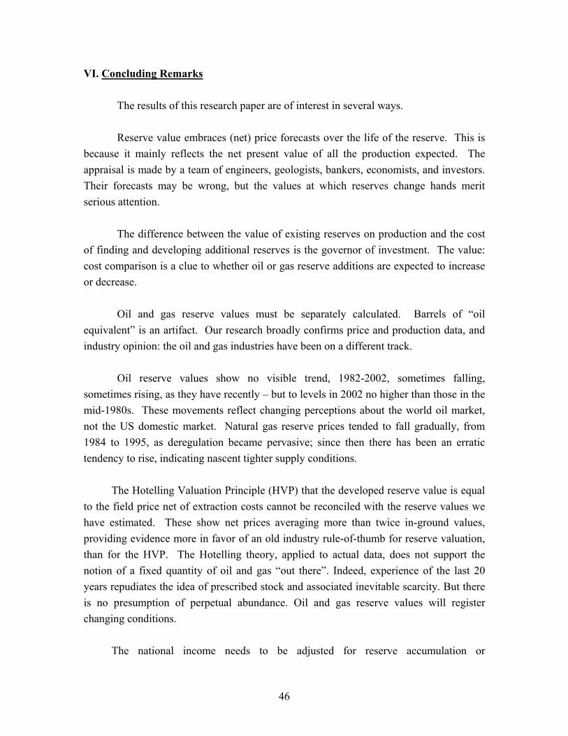
50
[Hotelling 1931] Harold Hotelling, “The Economics of Exhaustible Resources”, Journal of Political Economy, vol 39, pp 137-175.
[Jevons 1865] W. Stanley Jevons, The coal question; an inquiry concerning the progress
of the Nation, and the probable exhaustion of our coal-mines, (New York: A.M. Kelley) 1965.
[Krautkraemer 1998] J. A. Krautkraemer, “Nonrenewable Resource Scarcity”, Journal of
Economic Literature, vol. 36, pp 2065-2107. [Miller & Upton 1985] M.H. Miller and C.W. Upton, “A Test of the Hotelling Valuation
Principle,” Journal of Political Economy, 93 (1), 1985, 1-25. [Potter & Christy 1962] Neal Potter and F.T. Chrystie Jr., Trends in Natural Resource
Commodities. (Resources For The Future). [Smith & Ward 1981] J.L. Smith and G.L. Ward, “Maximum Likelihood Estimation of
the Size Distribution of North Sea Fields,” Mathematical Geology, 13 (5). [Solow 1974] Solow, R.M. “The Economics of Resources or the Resources of
Economics,” American Economic Review, Vol 64, pp1-14 [Stiglitz 1976] Joseph E. Stiglitz, “Monopoly and the Rate of Extraction of Exhaustible
Resources”, American Economic Review, 66 (Sept):655-661 (1976) p. 655. [Tilton 2003] John E. Tilton, On Borrowed Time? Assessing the Threat of Mineral
Depletion (Resources For The Future). [Watkins 1992] G.C. Watkins, “The Hotelling Principle: Autobahn or Cul de Sac” (IAEE
Presidential Address) The Energy Journal vol 13 no 1. [Watkins & Streifel 1998] G.C.Watkins and Shane Streifel “World Crude Oil Supply:
Evidence from Estimating Supply Functions by Country”, Journal of Energy Finance and Development, 3 (1), 23-48.
[Weeks 1969] Lewis G. Weeks, “Offshore Petroleum Development and Resources”,
Journal of Petroleum Technology, vol. 21, pp 377-85.
51
Appendix A:
Transaction Data
1 2 3 4 5 6 7 8 9 10
Year All Types Pure Oil Pure Gas All Types Pure Oil Pure Gas All Types Pure Oil Pure Gas
All Years 1563 341 416 107 33 29 1456 308 3871982 14 1 0 1 0 0 13 1 01983 22 2 1 1 0 0 21 2 11984 34 8 1 3 1 0 31 7 11985 35 5 4 1 0 0 34 5 41986 27 3 3 2 0 0 25 3 31987 51 12 5 2 2 0 49 10 51988 66 14 9 2 1 0 64 13 91989 104 19 18 5 1 0 99 18 181990 160 38 29 9 3 2 151 35 271991 101 20 18 7 1 0 94 19 181992 92 20 20 6 2 2 86 18 181993 122 28 28 7 1 2 115 27 261994 98 17 33 6 2 2 92 15 311995 124 35 33 10 5 2 114 30 311996 100 31 31 6 1 2 94 30 291997 72 16 27 5 3 1 67 13 261998 91 19 45 8 3 3 83 16 421999 62 13 26 5 1 2 57 12 242000 70 15 28 4 1 2 66 14 262001 61 11 21 9 2 5 52 9 162002 57 14 36 8 3 4 49 11 32
Source: The Scotia Group M&A Database, January 2003
Outliers are defined as follows:
For pure transactions, a reserve price more than two standard deviations for that year.For mixed transactions, a transaction value more than two standard deviations away from the fitted value.Transactions of value less than $0.55 per barrel or $0.10 per mcf, or greater than $27.50 per barrel or $5 per mcf.
Table A-1: Number of Identified Transactions
All Inclusive Number of Outliers Excluding Outliers
52
1 2 3 4 5 6 7 8 9
Year Mean Std. Dev. MedianCoeff. Of Variation Skewness Kurtosis Log Normality # Obs.
All Years 101.5 287.4 14.9 2.74 4.89 30.87 --- 15631982 480.4 1569.7 38.0 3.27 3.32 12.04 Not Rejected 141983 103.7 224.3 14.4 2.16 2.37 7.13 Not Rejected 221984 979.0 2918.8 39.2 2.98 3.32 12.93 Not Rejected 341985 232.5 913.1 17.4 3.93 5.41 31.07 Not Rejected 351986 133.7 243.6 10.5 1.82 1.99 5.98 Not Rejected 271987 36.9 100.4 7.0 2.72 4.89 28.99 Not Rejected 511988 95.4 343.2 7.2 3.60 6.22 44.65 Not Rejected 661989 40.8 106.5 8.1 2.61 5.51 38.79 Not Rejected 1041990 30.3 80.3 5.6 2.65 4.77 29.41 Not Rejected 1601991 29.1 85.2 5.0 2.92 4.71 25.56 Not Rejected 1011992 39.7 134.6 5.2 3.39 6.92 56.16 Not Rejected 921993 37.9 115.7 7.0 3.06 6.81 56.70 Not Rejected 1221994 38.8 90.6 9.7 2.33 4.02 20.01 Not Rejected 981995 32.8 74.5 8.3 2.27 4.09 21.61 Not Rejected 1241996 35.5 93.8 11.0 2.64 5.88 41.81 Not Rejected 1001997 120.1 238.2 26.4 1.98 4.22 24.18 Not Rejected 721998 114.0 494.6 17.0 4.34 6.41 42.60 Not Rejected 911999 35.0 54.8 14.5 1.57 2.65 9.38 Not Rejected 622000 216.2 600.3 23.9 2.78 4.73 25.84 Not Rejected 702001 298.7 721.9 53.5 2.42 3.45 14.78 Not Rejected 612002 178.4 326.1 62.0 1.83 2.97 11.89 Not Rejected 57
Source: The Scotia Group M&A Database, January 2003
The normality test used is Jarque-Bera; reject indicates that normality of the log distribution was rejected at 95% confidence level.
Table A-2: Summary Statistics for Transaction Values, All Transactions[Millions of Nominal $, where relevant]
53
1 2 3 4 5 6 7 8 9
Year Mean Std. Dev. MedianCoeff. Of Variation Skewness Kurtosis Log Normality # Obs.
All Years 46.8 91.0 13.6 1.73 2.89 12.53 --- 14561982 61.2 63.2 32.0 1.03 0.76 1.90 Not Rejected 131983 74.5 182.2 13.8 2.45 3.20 12.48 Not Rejected 211984 320.2 1047.2 33.7 3.27 4.66 24.10 Not Rejected 311985 80.5 161.2 16.8 2.00 2.97 11.02 Not Rejected 341986 78.2 143.2 10.1 1.83 1.86 4.89 Not Rejected 251987 19.8 35.8 6.0 1.81 2.81 10.23 Not Rejected 491988 56.3 142.9 6.7 2.54 3.66 15.73 Not Rejected 641989 28.3 59.7 8.0 2.11 4.99 34.37 Not Rejected 991990 16.8 32.3 5.0 1.93 3.12 12.33 Not Rejected 1511991 13.5 22.6 5.0 1.67 2.82 11.39 Not Rejected 941992 19.0 33.6 4.4 1.77 2.85 11.85 Not Rejected 861993 20.4 31.8 7.0 1.56 2.77 11.32 Not Rejected 1151994 20.0 29.6 8.2 1.48 2.59 9.95 Not Rejected 921995 19.1 31.2 8.0 1.64 2.89 11.29 Not Rejected 1141996 20.7 28.2 10.5 1.36 2.90 13.11 Not Rejected 941997 85.5 120.8 25.1 1.41 1.72 5.39 Not Rejected 671998 42.3 55.5 17.0 1.31 1.82 5.63 Not Rejected 831999 22.4 24.0 13.7 1.07 1.61 5.16 Not Rejected 572000 116.0 209.3 22.0 1.80 2.42 8.05 Not Rejected 662001 127.2 234.2 46.4 1.84 3.58 18.11 Not Rejected 522002 106.7 141.9 60.0 1.33 2.63 10.44 Not Rejected 49
Source: The Scotia Group M&A Database, January 2003
The normality test used is Jarque-Bera; reject indicates that normality of the log distribution was rejected at 95% confidence level.
Table A-3: Summary Statistics for Transaction Values, Excluding Outliers[Millions of Nominal $, where relevant]
54
1 2 3 4 5 6 7 8 9
Year Mean Std. Dev. MedianCoeff. Of Variation Skewness Kurtosis Log Normality # Obs.
1982 159.3 --- 159.3 --- --- --- --- 11983 14.0 17.6 14.0 1.26 0.00 1.00 Not Rejected 21984 263.4 633.7 18.7 2.41 2.04 5.16 Not Rejected 71985 8.3 10.4 4.2 1.25 1.34 3.01 Not Rejected 51986 32.9 43.9 15.0 1.33 0.62 1.50 Not Rejected 31987 4.2 6.6 1.7 1.56 2.43 7.34 Not Rejected 101988 79.6 189.3 2.9 2.38 2.48 7.80 Not Rejected 131989 21.3 47.5 3.5 2.23 3.15 12.06 Not Rejected 181990 10.1 27.6 1.3 2.72 4.72 25.64 Not Rejected 351991 14.6 24.1 2.9 1.65 1.70 4.19 Not Rejected 191992 12.3 28.4 2.4 2.30 2.95 10.56 Not Rejected 181993 13.8 15.1 7.8 1.09 1.55 4.89 Not Rejected 271994 19.7 29.7 6.2 1.51 2.00 6.07 Not Rejected 151995 18.4 39.4 2.6 2.14 2.95 10.61 Not Rejected 301996 19.5 33.5 8.7 1.72 3.44 15.44 Not Rejected 301997 93.2 122.0 18.7 1.31 1.08 2.46 Not Rejected 131998 48.9 51.4 36.3 1.05 1.46 4.78 Not Rejected 161999 15.1 21.4 7.5 1.42 1.79 4.71 Not Rejected 122000 57.5 106.6 11.6 1.85 2.32 7.51 Not Rejected 142001 21.3 35.0 4.0 1.64 1.62 4.19 Not Rejected 92002 157.0 213.3 58.0 1.36 1.98 5.94 Not Rejected 11
--- Insufficient data points.
Source: The Scotia Group M&A Database, January 2003
The normality test used is Jarque-Bera; reject indicates that normality of the log distribution was rejected at 95% confidence level.
Table A-4: Summary Statistics for Pure Oil Transaction Values, Excluding Outliers[Millions of Nominal $, where relevant]
55
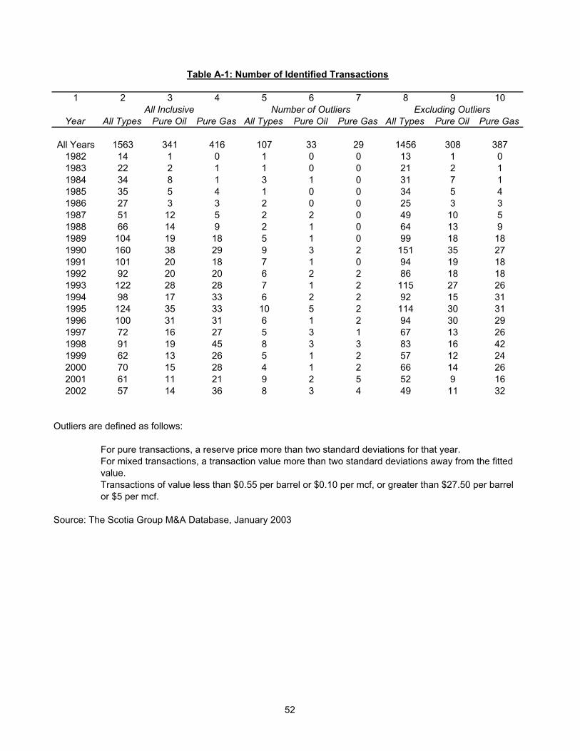
1 2 3 4 5 6 7 8 9
Year Mean Std. Dev. MedianCoeff. Of Variation Skewness Kurtosis Log Normality # Obs.
1982 --- --- --- --- --- --- --- 01983 7.5 --- 7.5 --- --- --- --- 11984 294.0 --- 294.0 --- --- --- --- 11985 72.0 54.9 64.8 0.76 0.43 1.97 Not Rejected 41986 137.6 231.6 4.3 1.68 0.71 1.50 Not Rejected 31987 9.2 7.9 7.3 0.86 1.10 2.77 Not Rejected 51988 83.1 237.0 3.2 2.85 2.47 7.12 Not Rejected 91989 25.0 40.8 5.7 1.63 2.22 6.74 Not Rejected 181990 18.1 31.1 4.3 1.72 2.25 7.01 Not Rejected 271991 26.5 38.5 9.4 1.45 1.57 3.97 Not Rejected 181992 9.5 14.5 3.1 1.52 2.02 6.46 Not Rejected 181993 28.2 41.1 6.6 1.38 2.08 7.12 Not Rejected 261994 20.3 34.1 7.4 1.68 2.82 11.00 Not Rejected 311995 24.9 31.2 11.4 1.25 1.94 5.80 Not Rejected 311996 24.5 29.8 12.1 1.22 2.20 7.34 Not Rejected 291997 58.6 95.3 22.6 1.55 2.26 6.80 Not Rejected 261998 42.5 49.8 19.8 1.17 1.71 5.55 Not Rejected 421999 26.6 26.7 18.2 1.35 1.34 4.25 Not Rejected 242000 146.8 227.6 44.3 1.55 2.11 6.55 Not Rejected 262001 130.7 220.9 36.4 1.69 1.87 5.17 Not Rejected 162002 92.5 123.0 56.8 1.33 2.18 7.21 Not Rejected 32
--- Insufficient data points.
Source: The Scotia Group M&A Database, January 2003
The normality test used is Jarque-Bera; reject indicates that normality of the log distribution was rejected at 95% confidence level.
Table A-5: Summary Statistics for Pure Natural Gas Transaction Values, Excluding Outliers[Millions of Nominal $, where relevant]
56

1 2 3 4 5 6 7 8 9
Year Mean Std. Dev. MedianCoeff. Of Variation Skewness Kurtosis Log Normality # Obs.
All Years 9.8 38.0 0.4 3.40 5.49 38.76 --- 15631982 53.3 181.7 1.7 3.41 3.32 12.04 Not Rejected 141983 12.8 28.8 0.8 2.25 2.24 6.54 Not Rejected 221984 137.3 477.7 2.0 3.48 3.66 14.69 Rejected 341985 24.2 115.6 0.6 4.78 5.54 32.14 Not Rejected 351986 7.4 16.5 0.4 2.22 2.96 11.55 Not Rejected 271987 4.7 16.8 0.5 3.62 4.85 25.69 Not Rejected 511988 5.7 18.6 0.6 3.27 4.92 27.53 Not Rejected 661989 2.2 4.4 0.5 2.02 4.00 22.74 Not Rejected 1041990 3.1 13.9 0.3 4.47 7.68 68.52 Not Rejected 1601991 2.2 7.5 0.2 3.44 6.18 46.48 Not Rejected 1011992 3.7 12.1 0.4 3.25 5.49 35.73 Not Rejected 921993 2.1 4.5 0.4 2.07 3.91 21.96 Not Rejected 1221994 3.6 10.8 0.3 3.00 5.20 33.14 Not Rejected 981995 3.8 16.1 0.3 4.17 8.37 81.30 Not Rejected 1241996 3.1 6.9 0.3 2.26 3.36 14.22 Not Rejected 1001997 12.8 47.4 0.8 3.70 6.96 54.47 Not Rejected 721998 20.6 118.7 0.0 5.76 7.10 54.08 Not Rejected 911999 1.9 5.3 0.3 2.86 5.20 33.12 Not Rejected 622000 22.2 111.2 0.3 5.02 6.54 46.88 Not Rejected 702001 5.8 13.4 0.3 2.31 4.08 22.07 Not Rejected 612002 9.3 24.2 0.0 2.61 3.65 16.56 Not Rejected 57
Table A-6: Summary Statistics for Size of Oil Reserves, All Transactions[Millions of Barrels, where relevant]
Source: The Scotia Group M&A Database, January 2003
The normality test used is Jarque-Bera; reject indicates that normality of the log distribution was rejected at 95% confidence level.
57
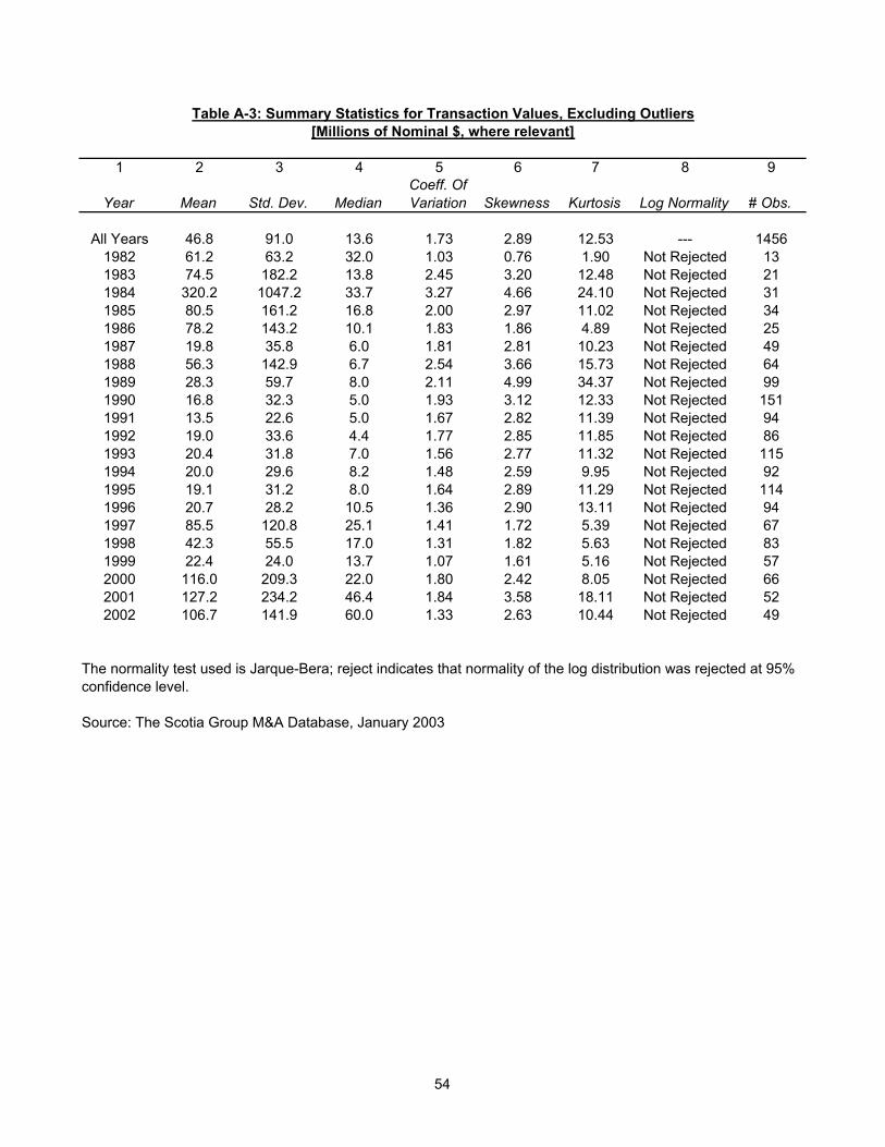
1 2 3 4 5 6 7 8 9
Year Mean Std. Dev. MedianCoeff. Of Variation Skewness Kurtosis Log Normality # Obs.
All Years 58.3 159.0 7.6 2.69 4.70 29.91 --- 15631982 178.3 564.7 9.9 3.17 3.27 11.82 Not Rejected 141983 59.9 181.0 3.6 3.02 3.78 16.34 Not Rejected 221984 414.1 1259.9 13.8 3.04 3.29 12.63 Not Rejected 341985 109.3 366.9 10.8 5.26 5.04 27.95 Not Rejected 351986 111.0 229.3 7.0 2.07 2.35 7.55 Not Rejected 271987 14.4 24.0 4.9 1.67 2.22 7.11 Not Rejected 511988 57.5 220.8 3.6 3.84 5.94 40.41 Not Rejected 661989 30.3 72.9 7.8 2.41 4.85 29.51 Not Rejected 1041990 23.3 80.5 3.2 3.45 7.57 68.64 Not Rejected 1601991 19.9 55.1 2.7 2.76 4.24 21.12 Not Rejected 1011992 26.7 94.5 4.0 3.54 6.09 40.45 Not Rejected 921993 26.9 63.5 3.9 2.36 3.85 19.30 Not Rejected 1221994 23.3 49.2 4.7 2.11 3.37 14.50 Not Rejected 981995 24.5 55.0 3.5 2.24 3.49 15.87 Not Rejected 1241996 24.6 54.8 4.9 2.23 5.42 40.05 Rejected 1001997 71.1 154.1 11.1 2.17 4.20 24.31 Not Rejected 721998 57.3 180.4 11.9 3.15 7.32 62.11 Rejected 911999 32.7 54.6 11.1 1.67 2.58 9.53 Not Rejected 622000 141.4 349.1 15.5 2.47 4.31 24.39 Not Rejected 702001 184.4 501.8 19.6 2.72 3.55 14.62 Not Rejected 612002 104.9 234.8 26.1 2.24 4.18 23.45 Not Rejected 57
Table A-7: Summary Statistics for Size of Natural Gas Reserves, All Transactions[BCFs, where relevant]
Source: The Scotia Group M&A Database, January 2003
The normality test used is Jarque-Bera; reject indicates that normality of the log distribution was rejected at 95% confidence level.
58
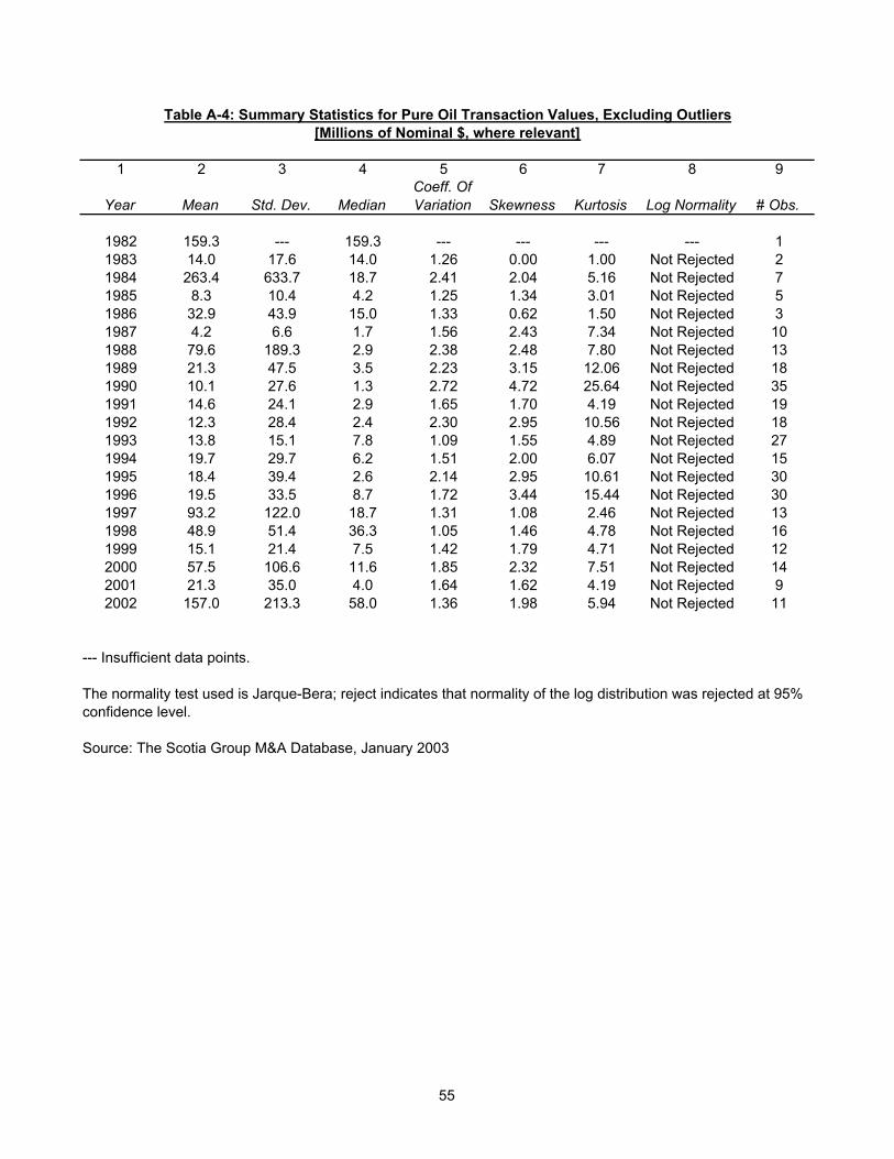
1 2 3 4 5 6 7 8 9
Year Mean Std. Dev. MedianCoeff. Of Variation Skewness Kurtosis Log Normality # Obs.
All Years 112.5 323.7 17.8 2.55 4.74 29.27 --- 15631982 471.4 1562.3 27.0 3.31 3.31 12.01 Not Rejected 141983 130.5 305.8 11.5 2.34 2.72 9.63 Not Rejected 221984 1169.4 3746.3 28.6 3.20 3.50 14.06 Not Rejected 341985 242.3 998.4 18.0 4.12 5.41 31.05 Not Rejected 351986 151.8 291.3 11.0 1.92 2.26 7.27 Not Rejected 271987 39.9 95.0 9.4 2.38 4.12 20.55 Not Rejected 511988 88.8 288.2 10.7 3.25 5.71 38.84 Not Rejected 661989 42.4 83.2 13.3 1.96 4.24 24.40 Not Rejected 1041990 40.4 119.9 8.1 2.97 5.55 37.44 Not Rejected 1601991 31.9 88.8 5.7 2.78 5.01 29.96 Not Rejected 1011992 47.1 144.4 8.1 3.07 6.23 45.98 Not Rejected 921993 38.7 79.1 11.6 2.04 3.94 19.44 Not Rejected 1221994 43.2 89.3 13.3 2.07 4.45 27.45 Not Rejected 981995 45.7 103.8 10.6 2.27 5.33 39.92 Not Rejected 1241996 41.4 78.4 17.5 1.89 5.57 41.67 Not Rejected 1001997 141.6 315.5 31.4 2.23 4.80 27.92 Not Rejected 721998 170.6 747.5 24.0 4.38 6.43 43.14 Not Rejected 911999 42.9 58.2 21.1 1.36 2.20 7.30 Not Rejected 622000 263.3 778.9 31.5 2.96 4.93 27.34 Not Rejected 702001 216.2 507.0 42.8 2.34 3.33 13.30 Not Rejected 612002 155.9 250.0 66.0 1.60 3.27 16.21 Not Rejected 57
Table A-8: Summary Statistics for Transaction Size in Thermal Equivalence, All Transactions[Trillion BTUs, where relevant]
Source: The Scotia Group M&A Database, January 2003
Trillion BTUs: 1 Trillion BTUs = 1 Billion Cubic Feet at 1,000 BTUs per cubic foot (TBTUs)Thermal equivalence factor of 5.5 million BTUs per barrel used.
The normality test used is Jarque-Bera; reject indicates that normality of the log distribution was rejected at 95% confidence level.
59
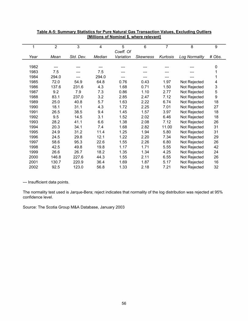
1 2 3 4 5 6 7 8 9
Year Mean Std. Dev. MedianCoeff. Of Variation Skewness Kurtosis Log Normality # Obs.
All Years 52.5 99.1 16.5 1.66 2.87 12.58 --- 14561982 54.4 84.9 26.3 1.56 2.35 7.64 Not Rejected 131983 107.3 293.0 9.7 2.73 3.26 12.65 Not Rejected 211984 298.6 1060.8 28.5 3.55 4.87 25.87 Not Rejected 311985 76.1 177.1 17.3 2.33 4.11 20.45 Not Rejected 341986 81.9 148.9 10.8 1.82 1.87 4.94 Not Rejected 251987 22.5 34.6 8.1 1.54 2.29 7.13 Not Rejected 491988 57.9 139.8 9.8 2.41 3.66 15.84 Not Rejected 641989 33.8 60.0 12.5 1.78 4.32 27.64 Not Rejected 991990 20.9 39.7 7.3 1.89 3.65 18.07 Not Rejected 1511991 16.2 25.6 5.5 1.58 2.72 10.99 Not Rejected 941992 24.6 39.3 7.4 1.59 2.55 9.60 Not Rejected 861993 25.8 36.3 11.0 1.41 2.36 8.75 Not Rejected 1151994 28.3 42.1 12.6 1.49 2.47 8.72 Not Rejected 921995 28.6 47.8 10.2 1.67 2.94 11.96 Rejected 1141996 30.9 36.3 17.1 1.17 1.92 6.41 Not Rejected 941997 94.4 121.5 30.0 1.29 1.70 5.90 Not Rejected 671998 61.0 87.5 23.8 1.43 2.61 11.00 Not Rejected 831999 31.0 34.1 21.0 1.10 1.89 6.48 Not Rejected 572000 137.5 243.7 23.9 1.77 2.71 10.57 Not Rejected 662001 99.7 165.9 44.8 1.66 4.00 22.68 Not Rejected 522002 110.9 144.8 59.9 1.31 2.04 6.52 Not Rejected 49
Table A-9: Summary Statistics for Transaction Size in Thermal Equivalence, Excluding Outliers[Trillion BTUs, where relevant]
Source: The Scotia Group M&A Database, January 2003
Trillion BTUs: 1 Trillion BTUs = 1 Billion Cubic Feet at 1,000 BTUs per cubic foot (TBTUs)Thermal equivalence factor of 5.5 million BTUs per barrel used.
The normality test used is Jarque-Bera; reject indicates that normality of the log distribution was rejected at 95% confidence level.
60
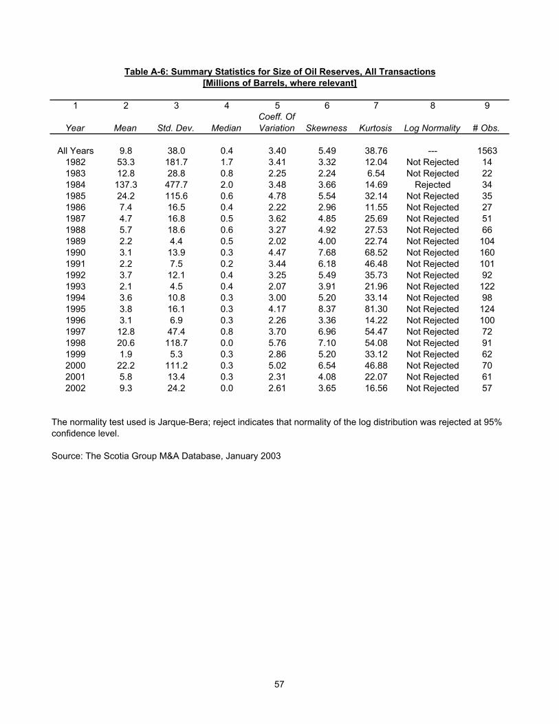
61
Appendix B: Estimates of Reserve Prices
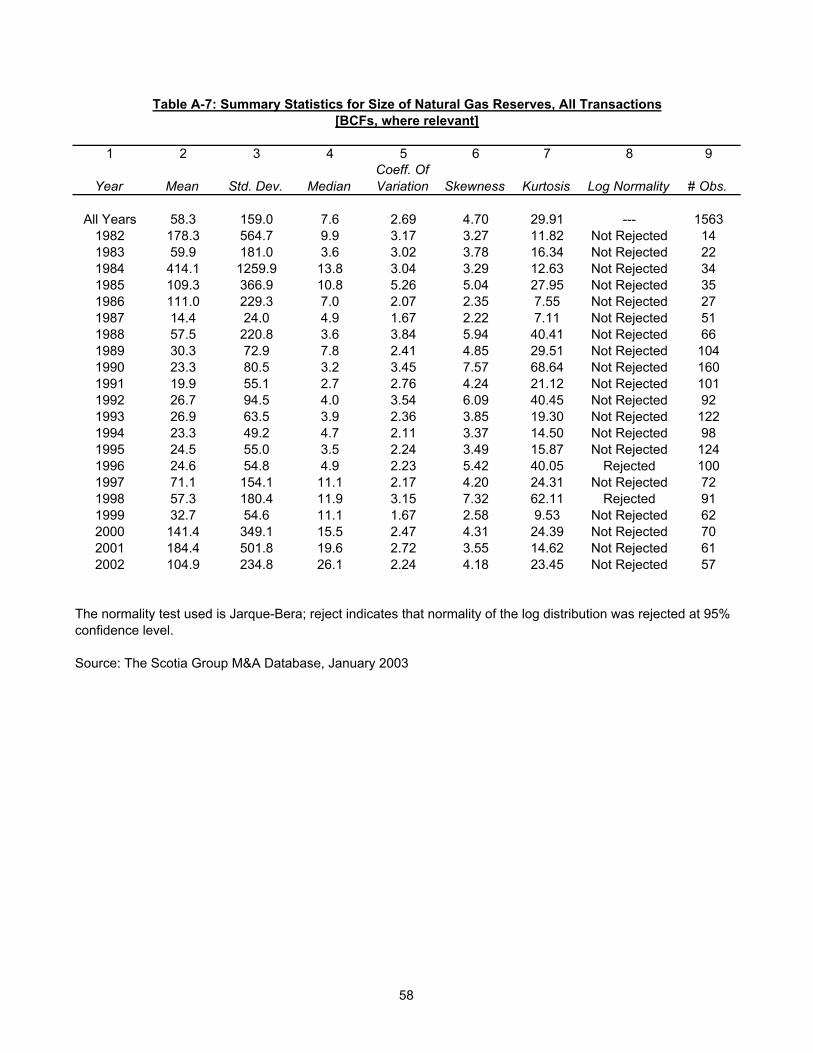
1 2 3 4 5 6 7
Year # ObsOil Coeff ($/bbl) t-stat
Gas Coeff ($/mcf) t-stat Adjusted R 2
1982 14 7.59 11.03 0.35 1.58 0.991983 22 4.35 6.89 0.65 6.19 0.921984 34 3.71 31.85 1.02 23.36 0.991985 35 5.62 12.72 0.73 5.38 0.991986 27 2.12 3.26 0.97 21.16 0.971987 51 5.60 27.45 0.94 7.38 0.941988 66 6.07 22.13 1.20 51.47 0.991989 104 4.60 5.38 1.21 22.58 0.881990 160 4.18 21.33 0.48 14.49 0.841991 101 3.35 11.18 1.16 28.97 0.971992 92 6.34 28.07 0.75 25.82 0.981993 122 2.60 2.26 1.49 18.08 0.831994 98 5.59 13.28 0.74 8.36 0.811995 124 3.16 24.01 0.88 24.44 0.911996 100 6.98 14.71 0.95 15.92 0.901997 72 2.88 19.48 1.13 26.45 0.951998 91 3.53 100.81 0.76 34.03 0.991999 62 4.97 13.38 0.86 26.30 0.942000 70 4.21 30.18 0.75 17.90 0.962001 61 5.63 5.41 1.42 49.83 0.982002 57 6.49 10.92 1.21 20.15 0.90
Note: Transaction values are regressed on reserves of oil (in bbls) and natural gas (in mcf).
Source: The Scotia Group M&A Database, January 2003
Table B-1a: Regression Results for All Transactions (No Constant)
62
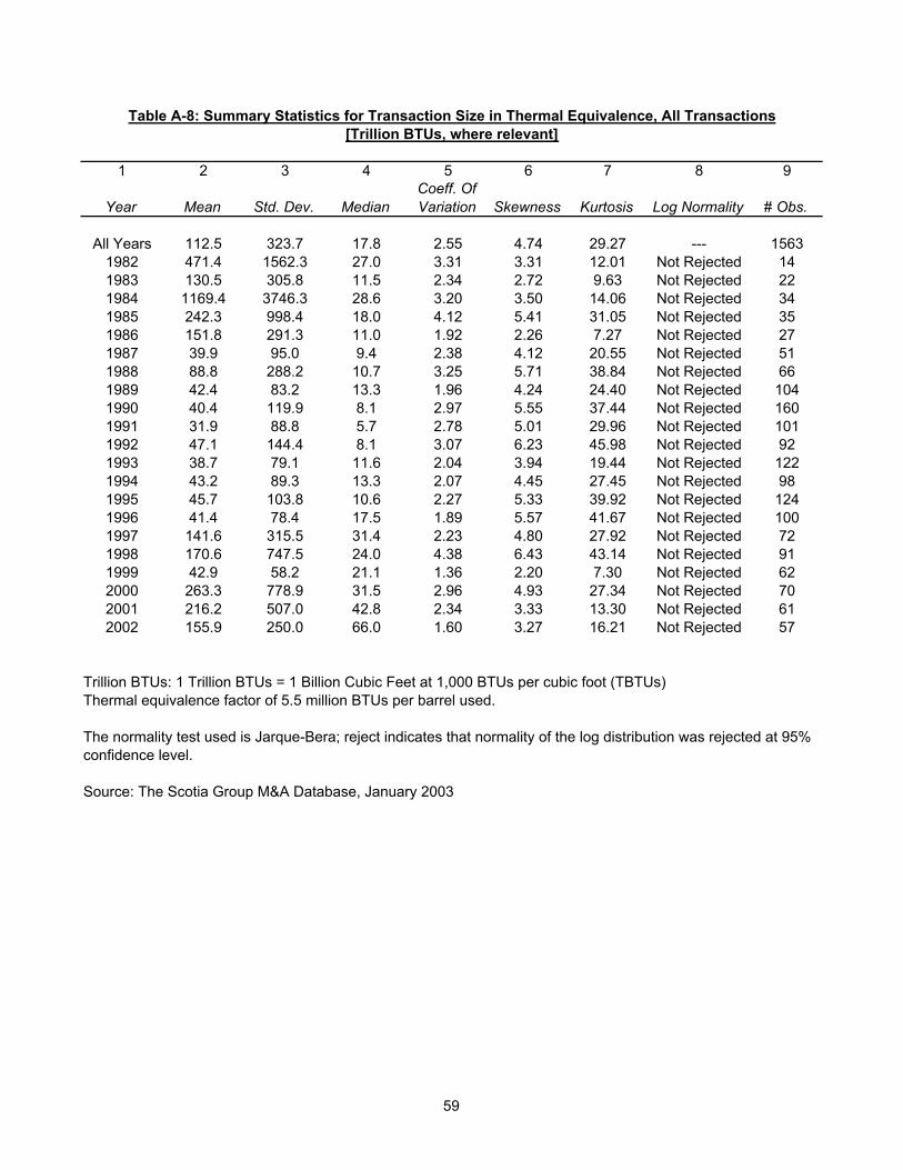
1 2 3 4 5 6 7 8 9
Year # Obs Constant t-statOil Coeff ($/bbl) t-stat
Gas Coeff ($/mcf) t-stat
Adjusted R 2
1982 14 16.54 1.36 7.79 11.44 0.28 1.26 0.991983 22 10.91 0.67 4.22 6.33 0.64 6.05 0.911984 34 53.79 1.76 3.70 32.83 1.01 23.55 0.991985 35 21.18 1.86 5.96 12.85 0.61 4.21 0.991986 27 12.79 1.31 1.96 3.01 0.96 20.48 0.971987 51 -3.70 -0.87 5.64 26.77 1.00 6.79 0.941988 66 -9.20 -2.05 6.17 22.65 1.21 52.64 0.991989 104 -8.15 -1.85 5.17 5.75 1.24 22.59 0.871990 160 6.82 2.42 4.10 20.94 0.46 13.68 0.821991 101 -1.42 -0.82 3.37 11.19 1.16 28.45 0.961992 92 -4.29 -1.87 6.41 28.38 0.76 26.21 0.981993 122 -9.92 -1.96 3.23 2.73 1.52 18.35 0.821994 98 1.76 0.36 5.57 12.99 0.73 7.69 0.771995 124 -1.24 -0.51 3.18 23.48 0.89 22.53 0.901996 100 -11.88 -3.60 7.41 15.99 1.01 17.21 0.901997 72 3.25 0.41 2.87 18.88 1.13 24.04 0.941998 91 -2.37 -0.60 3.53 100.39 0.76 32.92 0.991999 62 -3.73 -1.46 5.17 13.15 0.89 23.31 0.912000 70 19.49 1.21 4.20 30.05 0.73 16.48 0.962001 61 6.45 0.37 5.47 4.83 1.41 46.70 0.972002 57 -11.82 -0.65 6.65 10.25 1.23 18.30 0.87
Table B-1b: Regression Results for All Transactions (Constant Included)
Source: The Scotia Group M&A Database, January 2003
Note: Transaction values are regressed on reserves of oil (in bbls) and natural gas (in mcf).
63
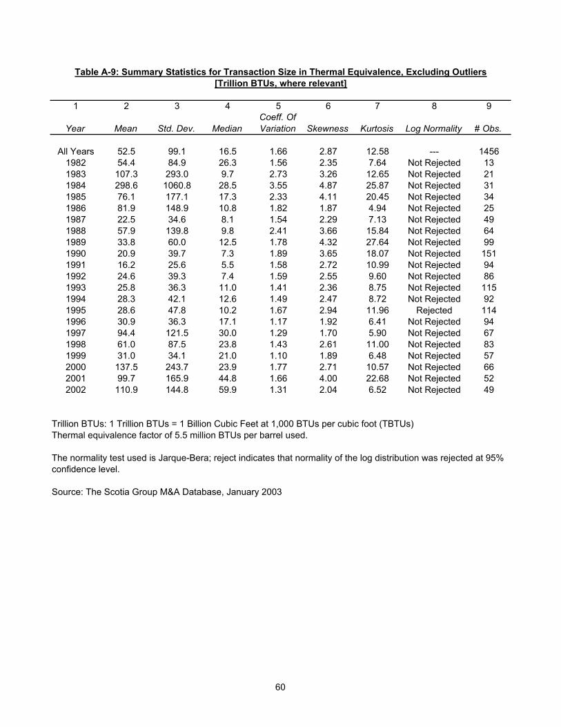
1 2 3 4 5 6
YearOil Coefficient
($/bbl) # Obs
Weighted ppb from Pure Oil Transactions
($/bbl) # Obs
Ratio of Estimated Oil Coefficient to Pure Transaction ppb
1982 7.59 14 7.11 1 1.071983 4.35 22 10.15 2 0.431984 3.71 34 6.93 8 0.531985 5.62 35 3.39 5 1.661986 2.12 27 8.86 3 0.241987 5.60 51 5.27 12 1.061988 6.07 66 6.44 14 0.941989 4.60 104 4.72 19 0.971990 4.18 160 4.50 38 0.931991 3.35 101 4.69 20 0.711992 6.34 92 4.75 20 1.341993 2.60 122 3.90 28 0.671994 5.59 98 7.70 17 0.731995 3.16 124 3.36 35 0.941996 6.98 100 5.36 31 1.301997 2.88 72 3.67 16 0.791998 3.53 91 3.40 19 1.041999 4.97 62 4.23 13 1.182000 4.21 70 4.07 15 1.042001 5.63 61 4.09 11 1.382002 6.49 57 5.52 14 1.18
Source: The Scotia Group M&A Database, January 2003
Table B-1c: Comparisons of Oil Regression Values with Pure Oil Values for All Transactions (No Constant)
Note: The pure oil value observations are weighted volumetrically by the barrels in each transaction for a given year. This is equivalent to summing the value of all pure transactions in a given year and dividing by the total volumes of oil reserves sold.
64
.1 2 3 4 5 6
Year Gas Coefficient ($/mcf) # Obs
Weighted ppmcf from Pure Gas Transactions
($/mcf) # Obs
Ratio of Estimated Gas Coefficient to Pure Transaction ppmcf
1982 0.35 14 --- 0 ---1983 0.65 22 1.05 1 0.621984 1.02 34 1.32 1 0.771985 0.73 35 1.34 4 0.551986 0.97 27 0.92 3 1.061987 0.94 51 0.89 5 1.051988 1.20 66 1.00 9 1.211989 1.21 104 1.18 18 1.031990 0.48 160 0.83 29 0.581991 1.16 101 0.90 18 1.281992 0.75 92 0.66 20 1.141993 1.49 122 0.73 28 2.041994 0.74 98 0.88 33 0.841995 0.88 124 0.75 33 1.181996 0.95 100 0.63 31 1.511997 1.13 72 0.93 27 1.221998 0.76 91 0.69 45 1.091999 0.86 62 0.85 26 1.022000 0.75 70 0.79 28 0.952001 1.42 61 1.43 21 0.992002 1.21 57 1.13 36 1.07
--- Insufficient data points.
Table B-1d: Comparisons of Natural Gas Regression Values with Pure Gas Values for All Transactions (No Constant)
Source: The Scotia Group M&A Database, January 2003
Note: The pure gas value observations are weighted volumetrically by the cubic feet in each transaction for a given year. This is equivalent to summing the value of all pure transactions in a given year and dividing by the total volumes of gas reserves sold.
65
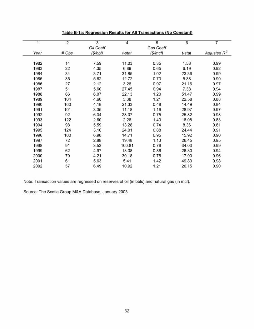
1 2 3 4 5 6 7
Year # ObsOil Coeff ($/bbl) t-stat
Gas Coeff ($/mcf) t-stat Adjusted R 2
1982 13 7.13 9.18 0.36 1.26 0.761983 21 3.37 39.87 0.64 58.92 0.991984 31 6.95 177.40 0.86 173.62 0.901985 34 7.74 1.66 0.52 1.05 0.891986 25 5.10 6.66 0.96 20.63 0.991987 49 4.40 6.48 1.02 6.96 0.921988 64 5.69 22.87 0.99 32.97 0.981989 99 4.61 3.56 0.88 5.75 0.821990 151 3.64 9.07 0.90 15.61 0.941991 94 4.44 12.36 0.87 29.63 0.961992 86 4.14 6.95 0.82 11.43 0.891993 115 3.54 15.00 0.87 13.45 0.941994 92 2.90 4.32 0.77 19.58 0.911995 114 3.81 16.85 0.60 9.93 0.951996 94 3.67 3.98 0.69 17.76 0.861997 67 5.01 14.24 0.93 15.52 0.921998 83 2.85 3.15 0.62 6.33 0.811999 57 3.59 6.31 0.67 7.39 0.882000 66 3.55 1.96 0.75 6.17 0.742001 52 4.21 4.76 1.68 9.71 0.952002 49 5.74 10.20 0.88 9.69 0.95
Table B-2a: Regression Results for All Transactions (No Constant), Excluding Outliers
Source: The Scotia Group M&A Database, January 2003
(with Robust Standard Errors, rather than OLS Standard Errors)
66
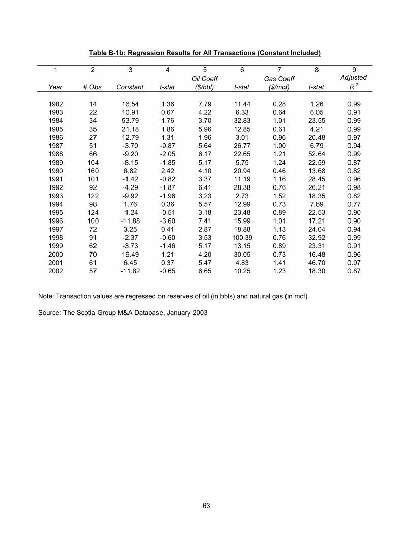
1 2 3 4 5 6 7 8 9
Year # Obs Constant t-statOil Coeff ($/bbl) t-stat
Gas Coeff ($/mcf) t-stat
Adjusted R 2
1982 13 26.09 1.99 5.71 4.57 0.28 1.32 0.651983 21 8.37 2.84 3.28 55.43 0.64 75.33 0.991984 31 16.29 2.80 6.88 157.34 0.86 227.36 0.901985 34 21.87 2.13 8.22 1.85 0.39 0.77 0.881986 25 0.33 0.11 5.09 6.91 0.96 18.74 0.981987 49 -2.29 -2.11 4.61 6.05 1.05 6.69 0.901988 64 -2.36 -1.22 5.72 23.13 0.99 35.14 0.981989 99 -1.13 -0.40 4.69 3.42 0.88 5.40 0.771990 151 -0.25 -0.46 3.65 8.84 0.90 14.80 0.921991 94 -0.30 -0.76 4.47 11.85 0.87 31.11 0.951992 86 -0.70 -0.53 4.17 6.77 0.83 11.36 0.861993 115 -0.20 -0.34 3.56 14.60 0.87 12.86 0.921994 92 1.49 1.69 2.82 4.12 0.75 18.20 0.871995 114 1.17 1.40 3.76 15.86 0.59 9.03 0.931996 94 -0.46 -0.33 3.71 3.65 0.69 16.38 0.781997 67 -2.70 -0.91 5.08 14.78 0.94 16.34 0.891998 83 9.76 2.68 2.54 2.86 0.57 5.65 0.721999 57 3.12 1.43 3.24 4.48 0.63 5.58 0.792000 66 21.40 2.16 3.17 1.81 0.71 5.85 0.672001 52 -10.25 -2.16 4.32 4.88 1.71 10.02 0.942002 49 3.82 0.63 5.67 9.18 0.86 8.11 0.92
Table B-2b: Regression Results for All Transactions (Constant Included), Excluding Outliers
Source: The Scotia Group M&A Database, January 2003
(with Robust Standard Errors, rather than OLS Standard Errors)
67
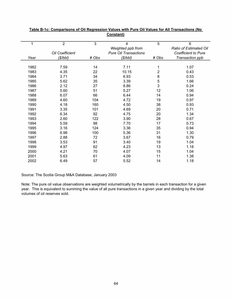
.1 2 3 4 5 6 7 8
YearConstant Included No Constant Ratio
Constant Included No Constant Ratio # Obs
1982 5.71 7.13 0.80 0.28 0.36 0.79 131983 3.28 3.37 0.97 0.64 0.64 0.99 211984 6.88 6.95 0.99 0.86 0.86 1.00 311985 8.22 7.74 1.06 0.39 0.52 0.74 341986 5.09 5.10 1.00 0.96 0.96 1.00 251987 4.61 4.40 1.05 1.05 1.02 1.03 491988 5.72 5.69 1.01 0.99 0.99 1.01 641989 4.69 4.61 1.02 0.88 0.88 1.01 991990 3.65 3.64 1.00 0.90 0.90 1.00 1511991 4.47 4.44 1.01 0.87 0.87 1.01 941992 4.17 4.14 1.01 0.83 0.82 1.01 861993 3.56 3.54 1.01 0.87 0.87 1.00 1151994 2.82 2.90 0.97 0.75 0.77 0.98 921995 3.76 3.81 0.99 0.59 0.60 0.98 1141996 3.71 3.67 1.01 0.69 0.69 1.01 941997 5.08 5.01 1.01 0.94 0.93 1.01 671998 2.54 2.85 0.89 0.57 0.62 0.92 831999 3.24 3.59 0.90 0.63 0.67 0.94 572000 3.17 3.55 0.89 0.71 0.75 0.95 662001 4.32 4.21 1.03 1.71 1.68 1.02 522002 5.67 5.74 0.99 0.86 0.88 0.98 49
Table B-2c: Effect of Including Constant on Regression Coeffcients(Excluding Outliers)
Source: The Scotia Group M&A Database, January 2003
Oil Coefficient ($/bbl) Gas Coefficient ($/mcf)
68
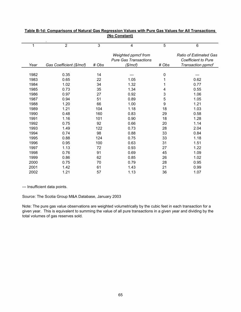
.1 2 3 4 5 6 7
Year All DataExcluding Outliers
Ratio 2/3 All Data
Excluding Outliers
Ratio 5/6
1982 7.59 7.13 1.06 0.35 0.36 0.971983 4.35 3.37 1.29 0.65 0.64 1.011984 3.71 6.95 0.53 1.02 0.86 1.181985 5.62 7.74 0.73 0.73 0.52 1.401986 2.12 5.10 0.42 0.97 0.96 1.011987 5.60 4.40 1.27 0.94 1.02 0.911988 6.07 5.69 1.07 1.20 0.99 1.221989 4.60 4.61 1.00 1.21 0.88 1.381990 4.18 3.64 1.15 0.48 0.90 0.531991 3.35 4.44 0.76 1.16 0.87 1.331992 6.34 4.14 1.53 0.75 0.82 0.911993 2.60 3.54 0.73 1.49 0.87 1.711994 5.59 2.90 1.93 0.74 0.77 0.961995 3.16 3.81 0.83 0.88 0.60 1.461996 6.98 3.67 1.90 0.95 0.69 1.391997 2.88 5.01 0.58 1.13 0.93 1.221998 3.53 2.85 1.24 0.76 0.62 1.231999 4.97 3.59 1.39 0.86 0.67 1.282000 4.21 3.55 1.19 0.75 0.75 1.002001 5.63 4.21 1.34 1.42 1.68 0.842002 6.49 5.74 1.13 1.21 0.88 1.37
Table B-2d: Effect of Outliers on Reserve Coefficients(No Constant)
Source: The Scotia Group M&A Database, January 2003
Oil Coefficient ($/bbl) Gas Coefficient ($/mcf)
69
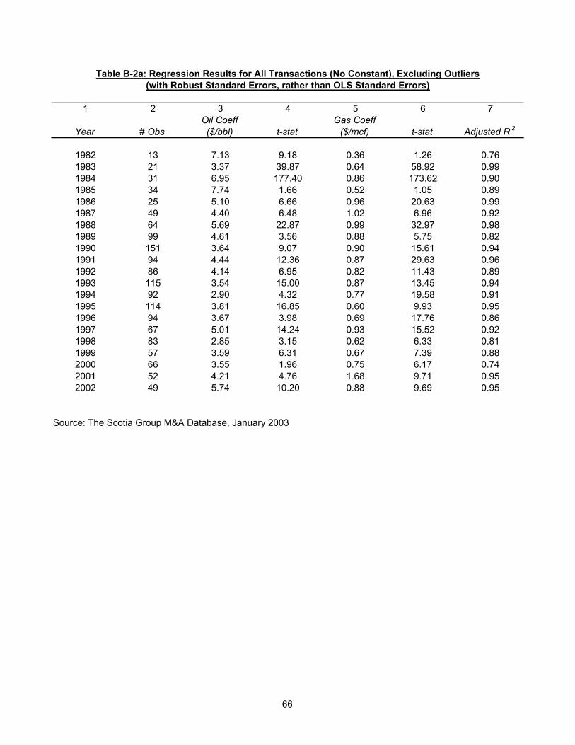
1 2 3 4 5 6
YearOil Coefficient
($/bbl) # Obs
Weighted ppb from Pure Oil Transactions
($/bbl) # Obs
Ratio of Estimated Oil Coefficient to Pure Transaction ppb
1982 7.13 13 7.11 1 1.001983 3.37 21 10.15 2 0.331984 6.95 31 6.94 7 1.001985 7.74 34 3.39 5 2.281986 5.10 25 8.86 3 0.581987 4.40 49 3.56 10 1.241988 5.69 64 6.15 13 0.931989 4.61 99 4.72 18 0.981990 3.64 151 4.22 35 0.861991 4.44 94 4.66 19 0.951992 4.14 86 3.46 18 1.201993 3.54 115 3.70 27 0.961994 2.90 92 3.71 15 0.781995 3.81 114 3.63 30 1.051996 3.67 94 3.84 30 0.961997 5.01 67 4.81 13 1.041998 2.85 83 3.34 16 0.851999 3.59 57 4.22 12 0.852000 3.55 66 3.46 14 1.032001 4.21 52 3.88 9 1.092002 5.74 49 5.19 11 1.11
Source: The Scotia Group M&A Database, January 2003
Table B-2e: Comparisons of Oil Regression Values (No Constant) with Pure Oil Values, Excluding Outliers
Note: The pure oil value observations are weighted volumetrically by the barrels in each transaction for a given year. This is equivalent to summing the value of all pure transactions in a given year and dividing by the total volumes of oil reserves sold.
70
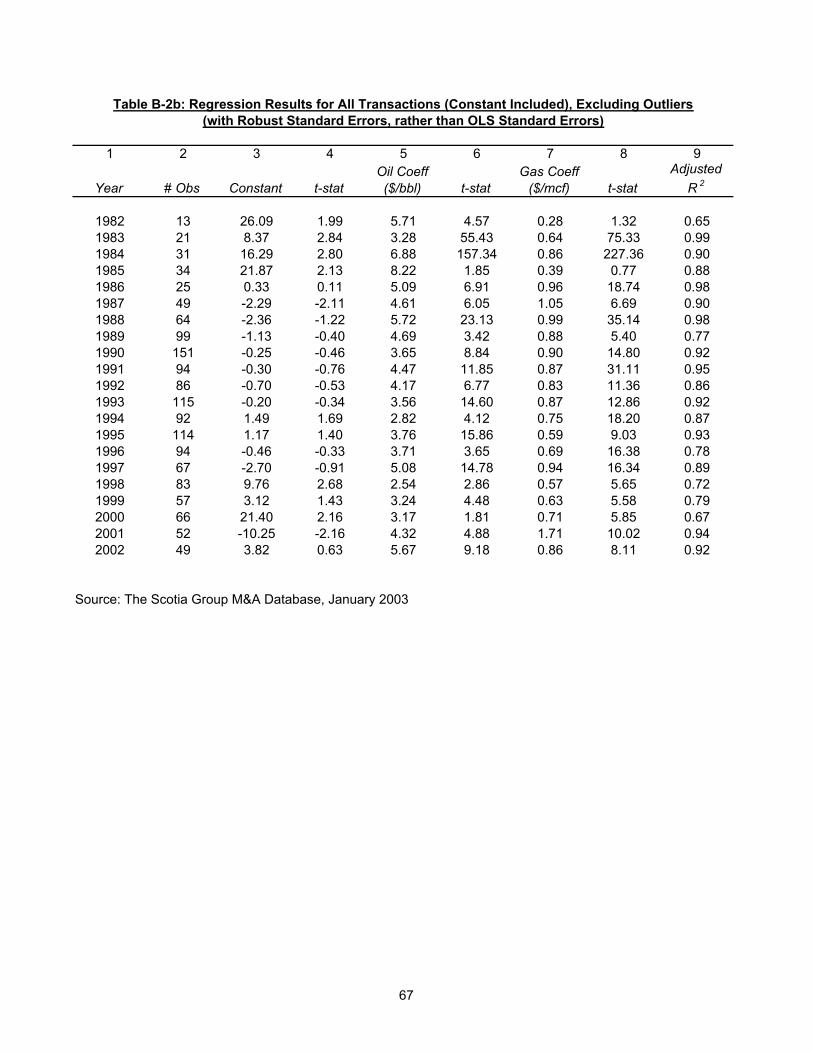
.1 2 3 4 5 6
Year Gas Coefficient ($/mcf) # Obs
Weighted ppmcf from Pure Gas Transactions
($/mcf) # Obs
Ratio of Estimated Gas Coefficient to Pure Transaction ppmcf
1982 0.36 13 --- 0 ---1983 0.64 21 1.05 1 0.611984 0.86 31 1.32 1 0.651985 0.52 34 1.34 4 0.391986 0.96 25 0.92 3 1.051987 1.02 49 0.89 5 1.151988 0.99 64 1.00 9 0.991989 0.88 99 1.18 18 0.741990 0.90 151 0.81 27 1.111991 0.87 94 0.90 18 0.961992 0.82 86 0.56 18 1.471993 0.87 115 0.77 26 1.131994 0.77 92 0.76 31 1.011995 0.60 114 0.70 31 0.871996 0.69 94 0.60 29 1.141997 0.93 67 0.90 26 1.031998 0.62 83 0.69 42 0.891999 0.67 57 0.83 24 0.822000 0.75 66 0.73 26 1.032001 1.68 52 1.55 16 1.082002 0.88 49 0.96 32 0.91
--- Insufficient data points.
Table B-2f: Comparisons of Natural Gas Regression Values (No Constant) with Pure Gas Values, Excluding Outliers
Source: The Scotia Group M&A Database, January 2003
Note: The pure gas value observations are weighted volumetrically by the cubic feet in each transaction for a given year. This is equivalent to summing the value of all pure transactions in a given year and dividing by the total volumes of gas reserves sold.
71
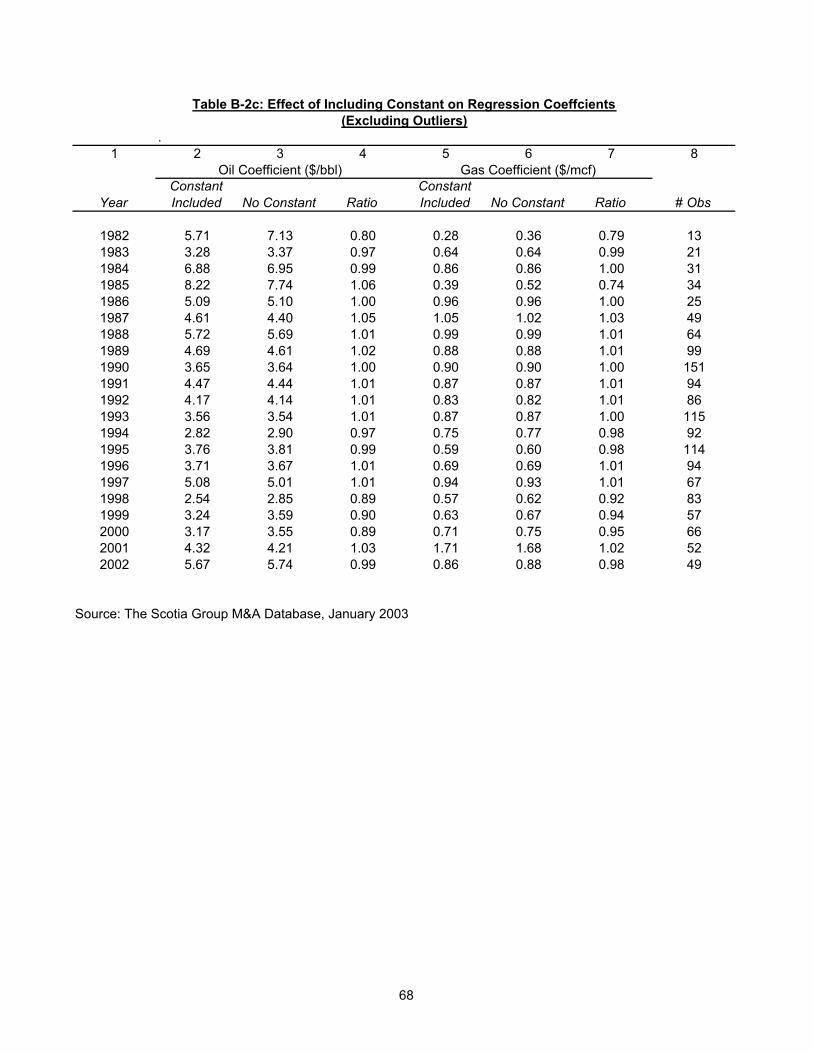
72
Appendix C: Auxiliary Data and Regressions
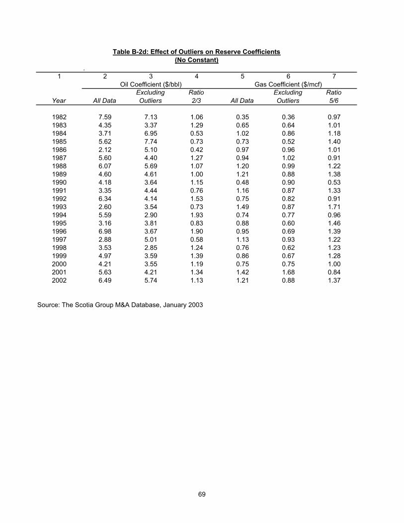
.1 2 3 4 5 6 7
Year
Beginning Year
ReservesAnnual
ProductionRatio 2/3
Beginning Year
ReservesAnnual
ProductionRatio 5/6
1982 29426 2950 10.0 201730 17506 11.51983 27858 3020 9.2 201512 15788 12.81984 27735 3037 9.1 200247 17193 11.61985 28446 3052 9.3 197463 15985 12.41986 28416 2973 9.6 193369 15610 12.41987 26889 2873 9.4 191586 16114 11.91988 27256 2811 9.7 187211 16670 11.21989 26825 2586 10.4 168024 16983 9.91990 26501 2505 10.6 167116 17233 9.71991 26254 2512 10.5 169346 17202 9.81992 24682 2446 10.1 167062 17423 9.61993 23745 2339 10.2 165015 17789 9.31994 22957 2268 10.1 162415 18322 8.91995 22457 2213 10.1 163837 17966 9.11996 22351 2173 10.3 165146 18861 8.81997 22017 2138 10.3 166474 19211 8.71998 22546 1991 11.3 167233 18720 8.91999 21034 1952 10.8 164041 18928 8.72000 21765 1880 11.6 167406 19219 8.72001 22045 1915 11.5 177427 19779 9.02002 22446 2106 10.7 183460 20351 9.0
Table C-1: Proven Reserves to Production Ratios
Source: EIA/DOE "US Crude Oil, Natural Gas, and Natural Gas Liquids Reserves"
Crude Oil (millions of barrels) Natural Gas (bcf)
Note: Beginning reserves indicate remaining reserves at January 1.
73

.1 2 3 4 5 6 7 8 9 10 11 12 13 14
Year a1 t-stat a2 t-stat a1 t-stat a2 t-statAdj. R 2
Total Obs
No. of Obs:
No Oil or Gas Prod
No. of Obs:
No Oil Prod
No. of Obs: No
Gas Prod
1982 7.13 4.02 --- --- 0.36 1.54 --- --- 0.72 13 13 13 131983 5.84 0.10 -2.47 -0.04 0.64 25.51 --- --- 0.99 21 20 20 211984 3.50 4.72 3.47 4.71 2.05 0.47 -0.94 -0.22 0.99 31 31 31 331985 -3.28 -0.04 12.46 0.16 1.38 2.51 -1.05 -1.76 0.89 34 32 32 321986 6.94 1.07 -1.82 -0.28 1.19 3.85 -0.24 -0.76 0.99 25 24 24 251987 4.44 1.06 -0.68 -0.16 0.80 3.83 0.33 1.42 0.92 49 41 41 441988 5.50 41.66 2.76 6.28 1.02 46.41 -0.25 -5.45 0.99 64 55 55 561989 5.15 2.94 -0.02 -0.01 1.02 16.29 -0.50 -4.62 0.85 99 85 87 891990 4.58 1.33 -0.96 -0.28 0.82 14.41 0.10 1.49 0.94 151 142 146 1491991 4.33 18.84 0.47 1.09 0.79 7.22 0.08 0.70 0.96 94 80 81 891992 4.18 10.23 0.08 0.13 0.78 9.34 0.11 0.90 0.89 86 57 63 671993 3.57 12.15 -0.57 -0.97 0.81 29.57 0.19 3.91 0.95 115 74 84 811994 3.14 12.81 -0.64 -1.38 0.79 24.20 -0.26 -2.38 0.91 92 53 63 551995 3.93 28.77 -1.20 -2.63 0.66 22.35 -0.07 -1.76 0.95 114 78 90 851996 4.01 14.34 -1.58 -2.53 0.74 16.77 -0.15 -1.83 0.87 94 57 67 631997 3.56 4.45 1.86 2.09 0.90 11.46 0.07 0.70 0.93 67 46 53 531998 1.81 5.21 3.01 5.00 0.80 13.77 -0.27 -3.85 0.87 83 46 68 541999 3.79 8.19 -0.56 -0.30 0.58 13.11 0.25 3.50 0.90 57 26 43 302000 6.02 3.10 -3.32 -1.48 0.77 11.06 -0.10 -0.83 0.74 66 29 50 342001 4.42 4.77 1.75 1.09 1.76 18.68 -0.42 -2.07 0.95 52 28 45 362002 5.55 9.19 0.23 0.34 1.06 9.48 -0.21 -1.77 0.95 49 27 47 36
--- Insufficient data points.
Note: Reserve status - whether reserves are on production or not.
Equation Specification:
where:adjprice is transaction price (after elimination of non reserve assets)the 'o' superscript denotes oilthe 'g' superscript denotes gasa1 and a2 are the two coefficients for each reserve being testedR denotes reserves soldD denotes dummy variable for reserves on production
Oil ($/bbl) Natural Gas ($/mcf)
Table C-2: Regression Results for Transactions with Information on Reserve Status (No Constant), Excluding Outliers
gggg
oooo RDaaRDaaadjprice ][][ 2121 +++=
74

.1 2 3 4 5 6 7 8 9 10 11
Year a1 t-stat a2 t-stat a1 t-stat a2 t-statAdjusted
R 2 Obs
1982 --- --- --- --- --- --- --- --- --- ---1983 --- --- --- --- --- --- --- --- --- ---1984 --- --- --- --- --- --- --- --- --- ---1985 --- --- --- --- --- --- --- --- --- ---1986 --- --- --- --- --- --- --- --- --- ---1987 --- --- --- --- --- --- --- --- --- ---1988 --- --- --- --- --- --- --- --- --- ---1989 11.00 3.35 -1.64 -2.00 0.80 4.30 0.03 1.17 0.97 171990 4.95 2.57 -0.39 -0.61 1.08 24.70 -0.04 -6.22 0.99 141991 --- --- --- --- --- --- --- --- --- ---1992 3.81 4.40 0.07 0.33 1.05 7.29 -0.08 -2.37 0.93 321993 3.85 10.11 -0.06 -1.15 1.21 20.16 -0.09 -7.22 0.97 461994 2.31 3.44 0.22 1.43 1.08 7.16 -0.07 -1.97 0.93 421995 5.00 7.57 -0.29 -1.66 0.72 8.49 -0.01 -0.77 0.97 421996 4.55 11.16 -0.01 -2.95 0.86 5.72 -0.02 -0.91 0.89 411997 5.00 5.35 -0.29 -1.73 0.93 25.56 0.00 -0.28 0.98 241998 5.68 8.14 -0.29 -5.62 1.06 13.96 -0.04 -2.97 0.95 421999 4.71 2.30 -0.16 -0.46 0.58 3.20 0.00 -0.03 0.86 322000 11.53 3.15 -0.66 -1.44 0.95 10.68 -0.03 -2.92 0.88 372001 3.22 1.49 0.16 0.36 2.47 17.12 -0.18 -5.76 0.96 322002 10.33 7.96 -0.99 -3.75 1.45 8.31 -0.08 -2.44 0.97 27
--- Insufficient data points.
Equation Specification:
where:adjprice is transaction price (after elimination of non reserve assets)the 'o' superscript denotes oilthe 'g' superscript denotes gasa1 and a2 are the two coefficients for each reserve being testedR denotes reserves soldH denotes the R/P ratio
R/P ratio is the ratio of remaining reserves to annual production.
Table C-3: Regression Results for Transactions with Information on R/P Ratios (No Constant), Excluding Outliers
Oil ($/bbl) Natural Gas ($/mcf)
gggg
oooo RHaaRHaaadjprice ][][ 2121 +++=
75
.1 2 3 4 5 6 7
Year Field Price Reserve PriceRatio 3/2 Field Price Reserve Price
Ratio 6/5
1982 28.52 7.13 0.250 2.46 0.36 0.1451983 26.19 3.37 0.129 2.59 0.64 0.2481984 25.88 6.95 0.268 2.66 0.86 0.3251985 24.09 7.74 0.321 2.51 0.52 0.2081986 12.51 5.10 0.408 1.94 0.96 0.4971987 15.40 4.40 0.286 1.67 1.02 0.6131988 12.58 5.69 0.452 1.69 0.99 0.5831989 15.86 4.61 0.291 1.69 0.88 0.5191990 20.03 3.64 0.182 1.71 0.90 0.5261991 16.54 4.44 0.268 1.64 0.87 0.5301992 15.99 4.14 0.259 1.74 0.82 0.4731993 14.25 3.54 0.248 2.04 0.87 0.4281994 13.19 2.90 0.220 1.85 0.77 0.4151995 14.62 3.81 0.261 1.55 0.60 0.3901996 18.46 3.67 0.199 2.17 0.69 0.3171997 17.23 5.01 0.291 2.32 0.93 0.4011998 10.87 2.85 0.262 1.96 0.62 0.3151999 15.56 3.59 0.231 2.19 0.67 0.3082000 26.72 3.55 0.133 3.69 0.75 0.2032001 21.84 4.21 0.193 4.12 1.68 0.4072002 22.51 5.74 0.255 2.95 0.88 0.298
Table C-4: Oil and Natural Gas Reserve and Field Prices
Source: EIA/DOE "Monthly Energy Review" June 2003
Oil ($/bbl) Natural Gas ($/mcf)
76
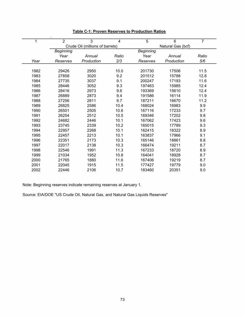
.1 2 3 4 5 6 7
Constant t-stat Coeff t-stat Adj. R 2 Obs
Oil Contemporary Price ($/bbl) 2.34 2.31 0.12 2.31 0.18 21Gas Contempory Price ($/mcf) 0.53 2.76 0.13 1.61 0.07 21
Oil 1 Period Lag Price ($/bbl) 2.35 2.50 0.11 2.33 0.19 20Gas 1 Period Lag Price ($/mcf) 0.55 3.05 0.14 1.75 0.10 20
Oil 2 Period Lag Price ($/bbl) 1.77 2.12 0.15 3.41 0.37 19Gas 2 Period Lag Price ($/mcf) 0.84 3.44 0.01 0.06 -0.06 19
Oil Contemporary Price ($/bbl) 4.43 15.24 -0.05 -0.79 -0.02 20Gas Contempory Price ($/mcf) 0.85 15.27 0.03 0.25 -0.05 20
Oil 1 Period Lag Price ($/bbl) 4.50 14.71 -0.01 -0.23 -0.06 19Gas 1 Period Lag Price ($/mcf) 0.83 18.08 0.34 3.28 0.35 19
Oil 2 Period Lag Price ($/bbl) 4.37 15.18 0.00 -0.01 -0.06 18Gas 2 Period Lag Price ($/mcf) 0.86 14.03 -0.04 -0.28 -0.06 18
Table C-5: Regression Results: Reserve Prices and Field Prices
Reserve Prices Against First Differences in Field Prices
Reserve Prices Against Field Prices
77
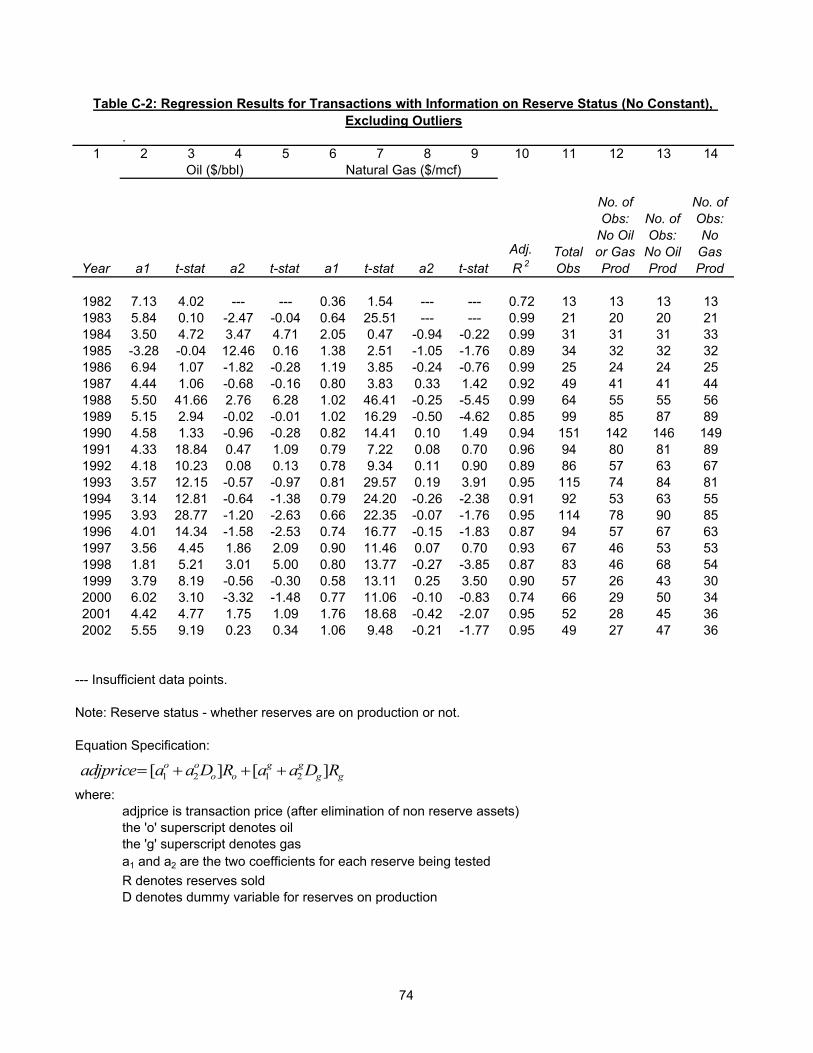
78
Appendix D: Hotelling Values, Implicit Price Expectations and Returns to Holding
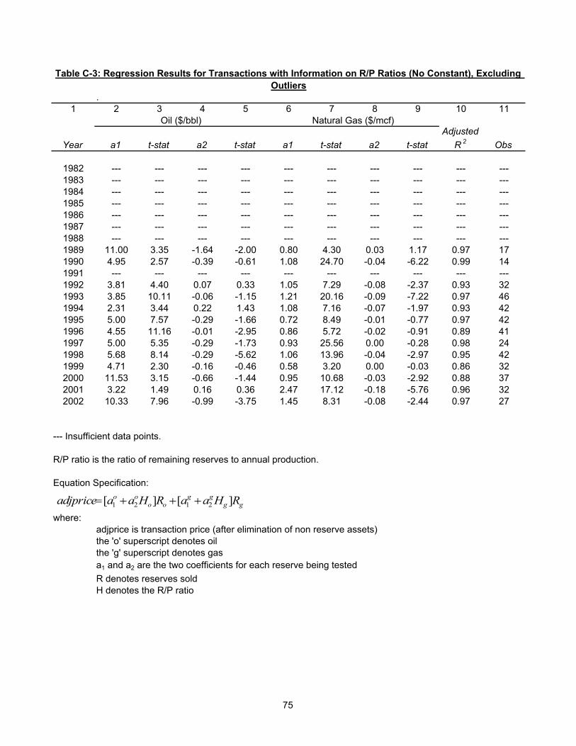
.1 2 3 4 5 6 7 8 9 10 11
YearP/R
RatioAdjusted Ratio (a)
Reserve Price (b)
$/bbl
SE of Reserve
Price $/bbl
Operating Cost (c)
$/bbl
Field Price (p)
$/bbl
Implicit Annual Growth Rate in Price
Net Field Price: HV
$/bbl
Ratio of HV to
Reserve Price
HV Spread
SDs
1982 0.10 0.09 7.13 0.78 9.98 28.52 0.12 18.54 2.60 14.71983 0.11 0.10 3.37 0.08 9.17 26.19 -0.17 17.02 5.05 161.41984 0.11 0.10 6.95 0.04 9.06 25.88 0.11 16.82 2.42 252.11985 0.11 0.10 7.74 4.66 8.43 24.09 0.11 15.66 2.02 1.71986 0.10 0.09 5.10 0.77 4.38 12.51 0.10 8.13 1.59 4.01987 0.11 0.10 4.40 0.68 5.39 15.40 0.05 10.01 2.27 8.31988 0.10 0.09 5.69 0.25 4.40 12.58 0.14 8.18 1.44 10.01989 0.10 0.09 4.61 1.30 5.55 15.86 0.06 10.31 2.23 4.41990 0.09 0.09 3.64 0.40 7.01 20.03 -0.05 13.02 3.58 23.41991 0.10 0.09 4.44 0.36 5.79 16.54 0.03 10.75 2.42 17.61992 0.10 0.09 4.14 0.60 5.60 15.99 0.01 10.39 2.51 10.51993 0.10 0.09 3.54 0.24 4.99 14.25 -0.03 9.26 2.62 24.31994 0.10 0.09 2.90 0.67 4.62 13.19 -0.03 8.57 2.96 8.51995 0.10 0.09 3.81 0.23 5.12 14.62 0.00 9.50 2.49 25.21996 0.10 0.09 3.67 0.92 6.46 18.46 -0.07 12.00 3.27 9.01997 0.10 0.09 5.01 0.35 6.03 17.23 0.02 11.20 2.24 17.61998 0.09 0.08 2.85 0.90 3.80 10.87 -0.01 7.07 2.48 4.71999 0.09 0.08 3.59 0.57 5.45 15.56 -0.04 10.11 2.82 11.52000 0.09 0.08 3.55 1.81 9.35 26.72 -0.19 17.37 4.89 7.62001 0.09 0.08 4.21 0.88 7.64 21.84 -0.09 14.20 3.37 11.32002 0.09 0.09 5.74 0.56 7.88 22.51 -0.04 14.63 2.55 15.8
Note: A value of 0.00 implies negligible growth rates.
(2)(3)(4)(5)(6)(7)(8)(9)(10)(11)
Net Field Price, p-c, Column (7) - Column (6).HV to Reserve Price, Column (9) / Column (4).HV Spread: Standard Deviations, [Column (9) - Column (4)] / Column (5).
Reserve Price (b), Table B-2a, Col 3.
Operating Cost (c), 35% of field price.Field Price (p), Table C-4.Implicit Annual Growth Rate in Price, see text.
Regression Results.
Table D-1: Estimates of Hotelling Values and Price Expectations, Oil
Sources:Production/Reserves Ratio, P/R, Table C-1.Adjusted Ratio (a), see text.
79
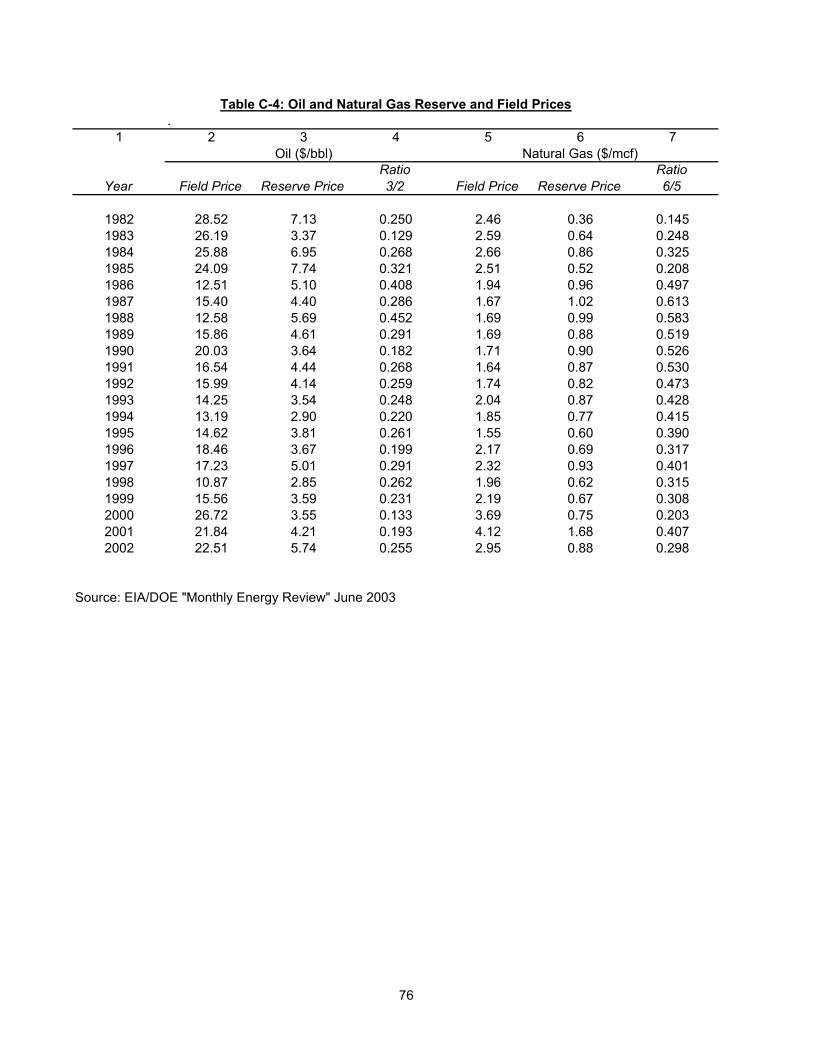
.1 2 3 4 5 6 7 8.00 9 10 11
YearP/R
RatioAdjusted Ratio (a)
Reserve Price (b)
$/bbl
SE of Reserve
Price $/bbl
Operating Cost (c)
$/bbl
Field Price (p)
$/bbl
Implicit Annual Growth Rate in Price
Net Field Price: HV
$/bbl
Ratio of HV to
Reserve Price
HV Spread
SDs
1982 0.10 0.09 7.11 --- 9.98 28.52 0.12 18.54 2.61 ---1983 0.11 0.10 10.15 3.38 9.17 26.19 0.16 17.02 1.68 2.01984 0.11 0.10 6.94 0.47 9.06 25.88 0.11 16.82 2.43 21.01985 0.11 0.10 3.39 2.24 8.43 24.09 -0.13 15.66 4.62 5.51986 0.10 0.09 8.86 1.95 4.38 12.51 0.16 8.13 0.92 -0.41987 0.11 0.10 3.56 2.03 5.39 15.40 -0.01 10.01 2.81 3.21988 0.10 0.09 6.15 1.62 4.40 12.58 0.15 8.18 1.33 1.31989 0.10 0.09 4.72 1.50 5.55 15.86 0.07 10.31 2.19 3.71990 0.09 0.09 4.22 1.71 7.01 20.03 -0.01 13.02 3.08 5.21991 0.10 0.09 4.66 1.89 5.79 16.54 0.04 10.75 2.31 3.21992 0.10 0.09 3.46 1.59 5.60 15.99 -0.04 10.39 3.01 4.41993 0.10 0.09 3.70 2.01 4.99 14.25 -0.02 9.26 2.50 2.81994 0.10 0.09 3.71 2.93 4.62 13.19 0.02 8.57 2.31 1.71995 0.10 0.09 3.63 1.45 5.12 14.62 -0.01 9.50 2.62 4.11996 0.10 0.09 3.84 2.09 6.46 18.46 -0.06 12.00 3.12 3.91997 0.10 0.09 4.81 2.60 6.03 17.23 0.01 11.20 2.33 2.51998 0.09 0.08 3.34 1.87 3.80 10.87 0.02 7.07 2.11 2.01999 0.09 0.08 4.22 1.71 5.45 15.56 0.00 10.11 2.40 3.42000 0.09 0.08 3.46 2.26 9.35 26.72 -0.20 17.37 5.02 6.12001 0.09 0.08 3.88 1.35 7.64 21.84 -0.11 14.20 3.66 7.62002 0.09 0.09 5.19 2.08 7.88 22.51 -0.06 14.63 2.82 4.5
--- Insufficient data points.
Note: A value of 0.00 implies negligible growth rates.
(2)(3)(4)(5)(6)(7)(8)(9)(10)(11)
Implicit Annual Growth Rate in Price, see text.Net Field Price, p-c, Column (7) - Column (6).HV to Reserve Price, Column (9) / Column (4).HV Spread: Standard Deviations, [Column (9) - Column (4)] / Column (5).
Reserve Price (b), Table B-2e, Col 4.
Operating Cost (c), 35% of field price.Field Price (p), Table C-4.
Table D-2: Estimates of Hotelling Values and Price Expectations, Pure Oil
Sources:Production/Reserves Ratio, P/R, Table C-1.Adjusted Ratio (a), see text.
Statistical Results.
80
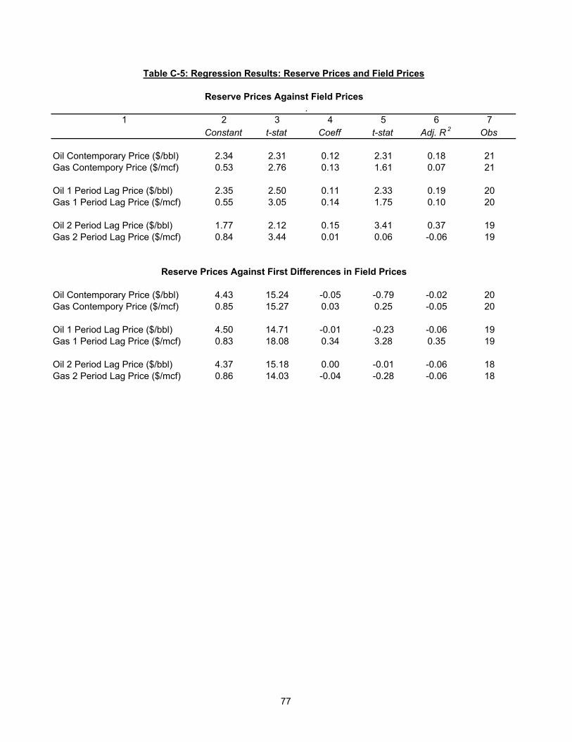
.1 2 3 4 5 6 7 8 9 10 11
YearP/R
RatioAdjusted Ratio (a)
Reserve Price (b)
$/mcf
SE of Reserve
Price $/mcf
Operating Cost (c) $/mcf
Field Price (p)
$/mcf
Implicit Annual Growth Rate in Price
Net Field Price: HV
$/mcf
Ratio of HV to
Reserve Price
HV Spread
SDs
1982 0.09 0.08 0.36 0.28 0.86 2.46 -0.02 1.60 4.48 4.41983 0.08 0.07 0.64 0.01 0.91 2.59 0.10 1.68 2.62 95.51984 0.09 0.08 0.86 0.00 0.93 2.66 0.17 1.73 2.00 173.71985 0.08 0.07 0.52 0.50 0.88 2.51 0.05 1.63 3.12 2.21986 0.08 0.07 0.96 0.05 0.68 1.94 0.13 1.26 1.31 6.31987 0.08 0.08 1.02 0.15 0.58 1.67 0.16 1.09 1.06 0.41988 0.09 0.08 0.99 0.03 0.59 1.69 0.17 1.10 1.11 3.81989 0.10 0.09 0.88 0.15 0.59 1.69 0.15 1.10 1.25 1.51990 0.10 0.09 0.90 0.06 0.60 1.71 0.15 1.11 1.24 3.71991 0.10 0.09 0.87 0.03 0.57 1.64 0.14 1.07 1.23 6.71992 0.10 0.09 0.82 0.07 0.61 1.74 0.11 1.13 1.37 4.31993 0.11 0.10 0.87 0.06 0.71 2.04 0.07 1.33 1.52 7.01994 0.11 0.10 0.77 0.04 0.65 1.85 0.08 1.20 1.57 11.11995 0.11 0.10 0.60 0.06 0.54 1.55 0.07 1.01 1.67 6.61996 0.11 0.10 0.69 0.04 0.76 2.17 0.02 1.41 2.05 18.71997 0.12 0.10 0.93 0.06 0.81 2.32 0.06 1.51 1.62 9.61998 0.11 0.10 0.62 0.10 0.69 1.96 0.00 1.27 2.06 6.71999 0.12 0.10 0.67 0.09 0.77 2.19 0.00 1.42 2.11 8.22000 0.11 0.10 0.75 0.12 1.29 3.69 -0.10 2.40 3.21 13.62001 0.11 0.10 1.68 0.17 1.44 4.12 0.04 2.68 1.60 5.82002 0.11 0.10 0.88 0.09 1.03 2.95 -0.02 1.92 2.18 11.5
Note: A value of 0.00 implies negligible growth rates.
(2)(3)(4)(5)(6)(7)(8)(9)(10)(11)
Net Field Price, p-c, Column (7) - Column (6).HV to Reserve Price, Column (9) / Column (4).HV Spread: Standard Deviations, [Column (9) - Column (4)] / Column (5).
Reserve Price (b), Table B-2a, Col 5.
Operating Cost (c), 35% of field price.Field Price (p), Table C-4.Implicit Annual Growth Rate in Price, see text.
Regression Results.
Table D-3: Estimates of Hotelling Values and Price Expectations, Natural Gas
Sources:Production/Reserves Ratio, P/R, Table C-1.Adjusted Ratio (a), see text.
81
.1 2 3 4 5 6 7 8 9 10 11
YearP/R
RatioAdjusted Ratio (a)
Reserve Price (b)
$/mcf
SE of Reserve
Price $/mcf
Operating Cost (c) $/mcf
Field Price (p)
$/mcf
Implicit Annual Growth Rate in Price
Net Field Price: HV
$/mcf
Ratio of HV to
Reserve Price
HV Spread
SDs
1982 0.09 0.08 --- --- 0.86 2.46 --- 1.60 --- ---1983 0.08 0.07 1.05 --- 0.91 2.59 0.18 1.68 1.61 ---1984 0.09 0.08 1.32 --- 0.93 2.66 0.23 1.73 1.31 ---1985 0.08 0.07 1.34 11.01 0.88 2.51 0.20 1.63 1.22 0.01986 0.08 0.07 0.92 0.18 0.68 1.94 0.13 1.26 1.37 1.91987 0.08 0.08 0.89 0.34 0.58 1.67 0.15 1.09 1.22 0.61988 0.09 0.08 1.00 0.27 0.59 1.69 0.17 1.10 1.10 0.41989 0.10 0.09 1.18 0.59 0.59 1.69 0.18 1.10 0.93 -0.11990 0.10 0.09 0.81 0.29 0.60 1.71 0.14 1.11 1.37 1.01991 0.10 0.09 0.90 0.35 0.57 1.64 0.14 1.07 1.18 0.51992 0.10 0.09 0.56 0.21 0.61 1.74 0.04 1.13 2.02 2.71993 0.11 0.10 0.77 0.28 0.71 2.04 0.05 1.33 1.71 2.01994 0.11 0.10 0.76 0.34 0.65 1.85 0.08 1.20 1.58 1.31995 0.11 0.10 0.70 0.24 0.54 1.55 0.09 1.01 1.45 1.31996 0.11 0.10 0.60 0.17 0.76 2.17 -0.01 1.41 2.35 4.61997 0.12 0.10 0.90 0.33 0.81 2.32 0.06 1.51 1.68 1.81998 0.11 0.10 0.69 0.29 0.69 1.96 0.02 1.27 1.85 2.01999 0.12 0.10 0.83 0.60 0.77 2.19 0.04 1.42 1.72 1.02000 0.11 0.10 0.73 0.48 1.29 3.69 -0.11 2.40 3.29 3.52001 0.11 0.10 1.55 0.56 1.44 4.12 0.03 2.68 1.73 2.02002 0.11 0.10 0.96 0.51 1.03 2.95 -0.01 1.92 1.99 1.9
--- Insufficient data points.
Note: A value of 0.00 implies negligible growth rates.
(2)(3)(4)(5)(6)(7)(8)(9)(10)(11)
Net Field Price, p-c, Column (7) - Column (6).HV to Reserve Price, Column (9) / Column (4).HV Spread: Standard Deviations, [Column (9) - Column (4)] / Column (5).
Reserve Price (b), Table B-2f, Col 4.
Operating Cost (c), 35% of field price.Field Price (p), Table C-4.Implicit Annual Growth Rate in Price, see text.
Statistical Results.
Table D-4: Estimates of Hotelling Values and Price Expectations, Pure Natural Gas
Sources:Production/Reserves Ratio, P/R, Table C-1.Adjusted Ratio (a), see text.
82
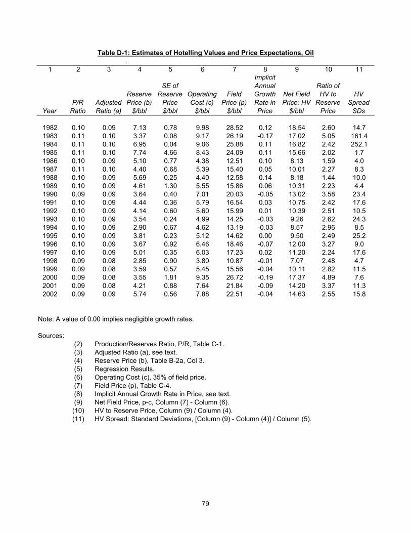
1 2 3 4 5 6
Year
Implicit Annual Growth Rate in
Price (g) Lower Bound Upper Bound Lower Bound Upper Bound
1982 0.12 0.05 0.16 0.06 0.171983 -0.17 -0.20 -0.15 -0.19 -0.141984 0.11 0.11 0.11 0.11 0.111985 0.11 -2.42 0.22 -0.12 0.351986 0.10 0.03 0.13 0.05 0.141987 0.05 -0.05 0.10 -0.02 0.111988 0.14 0.12 0.15 0.12 0.151989 0.06 -0.19 0.13 -0.05 0.171990 -0.05 -0.14 0.01 -0.12 0.021991 0.03 -0.01 0.06 0.00 0.071992 0.01 -0.09 0.06 -0.06 0.071993 -0.03 -1.29 0.00 -0.06 0.001994 -0.03 -0.26 0.05 -0.15 0.091995 0.00 -0.03 0.02 -0.03 0.031996 -0.07 -0.36 0.03 -0.21 0.071997 0.02 -0.01 0.04 -0.01 0.051998 -0.01 -0.36 0.06 -0.14 0.111999 -0.04 -0.15 0.02 -0.12 0.042000 -0.19 -2.29 0.01 -0.58 0.212001 -0.09 -0.28 -0.01 -0.20 0.022002 -0.04 -0.09 0.00 -0.08 0.00
Note: A value of 0.00 implies negligible growth rates.
Sources:(2)(3) See text.(4) See text.(5) See text.(6) See text.
The Scotia Group M&A Database, January 2003
Table D-5: Confidence Limits for Implicit Growth Rate of Oil Prices
Variance of V Method Delta Method
Implicit Annual Growth Rate in Price, Table D-1, Col 8.
83
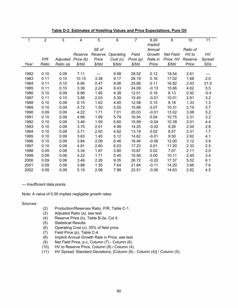
1 2 3 4 5 6
Year
Implicit Annual Growth Rate in
Price (g) Lower Bound Upper Bound Lower Bound Upper Bound
1982 -0.02 -0.93 0.20 -0.58 0.551983 0.10 0.10 0.11 0.10 0.111984 0.17 0.17 0.17 0.17 0.171985 0.05 -0.93 0.21 -0.39 0.501986 0.13 0.12 0.14 0.12 0.141987 0.16 0.13 0.18 0.14 0.191988 0.17 0.16 0.17 0.16 0.171989 0.15 0.09 0.18 0.11 0.191990 0.15 0.13 0.16 0.13 0.161991 0.14 0.13 0.14 0.13 0.141992 0.11 0.08 0.12 0.08 0.131993 0.07 0.04 0.09 0.05 0.091994 0.08 0.07 0.10 0.07 0.101995 0.07 0.03 0.09 0.03 0.101996 0.02 0.00 0.04 0.00 0.051997 0.06 0.04 0.08 0.04 0.091998 0.00 -0.10 0.05 -0.07 0.061999 0.00 -0.08 0.05 -0.06 0.062000 -0.10 -0.26 -0.02 -0.21 0.002001 0.04 0.00 0.07 0.01 0.072002 -0.02 -0.08 0.01 -0.07 0.02
Note: A value of 0.00 implies negligible growth rates.
Sources:(2)(3) See text.(4) See text.(5) See text.(6) See text.
Implicit Annual Growth Rate in Price, Table D-3, Col 8.
The Scotia Group M&A Database, January 2003
Table D-6: Confidence Limits for Implicit Growth Rate of Natural Gas Prices
Variance of V Method Delta Method
84

1 2 3 4 5 6 7 8 9
Year
Riskless Rate
(1-yr TB)Oil Value
($/bbl)Return to Holding
Oil Achieved Risk
PremiumGas Value
($/mcf)Return to Holding
Natural Gas Achieved
Risk Premium
Required Risk
Premium
1982 7.13 0.361983 0.096 3.37 -0.527 -0.623 0.64 0.800 0.704 0.1111984 0.109 6.95 1.061 0.952 0.86 0.345 0.236 0.1251985 0.084 7.74 0.114 0.030 0.52 -0.395 -0.479 0.1061986 0.065 5.10 -0.341 -0.406 0.96 0.843 0.779 0.0771987 0.068 4.40 -0.136 -0.204 1.02 0.062 -0.005 0.0841988 0.077 5.69 0.292 0.215 0.99 -0.038 -0.114 0.0891989 0.085 4.61 -0.189 -0.274 0.88 -0.111 -0.196 0.0851990 0.079 3.64 -0.211 -0.290 0.90 0.026 -0.053 0.0861991 0.059 4.44 0.219 0.160 0.87 -0.033 -0.092 0.0791992 0.039 4.14 -0.067 -0.106 0.82 -0.054 -0.093 0.0701993 0.034 3.54 -0.145 -0.179 0.87 0.060 0.026 0.0591994 0.053 2.90 -0.180 -0.234 0.77 -0.121 -0.174 0.0711995 0.059 3.81 0.315 0.255 0.60 -0.213 -0.272 0.0661996 0.055 3.67 -0.036 -0.091 0.69 0.138 0.082 0.0641997 0.056 5.01 0.362 0.306 0.93 0.356 0.300 0.0641998 0.051 2.85 -0.431 -0.482 0.62 -0.337 -0.388 0.0531999 0.051 3.59 0.260 0.209 0.67 0.092 0.041 0.0572000 0.061 3.55 -0.010 -0.071 0.75 0.110 0.049 0.0602001 0.035 4.21 0.185 0.150 1.68 1.241 1.206 0.0502002 0.020 5.74 0.364 0.344 0.88 -0.476 -0.496 0.046
Mean 0.062 0.045 -0.017 0.115 0.053 0.075St.Dev. 0.022 0.358 0.356 0.429 0.427 0.021St.Err. 0.005 0.080 0.080 0.096 0.095 0.005Mn/Se 12.578 0.560 -0.213 1.197 0.556 15.975
Sources:(2) Federal Reserve Board Historical Rates (http://www.federalreserve.gov/releases/h15/data/a/tcm1y.txt)(3) Oil Reserve Price, Table B-2a, Col 3.(4) Percentage Change, Col 3 (t)/Col 3 (t-1) - 1(5) Oil Achieved Risk Premium, Col 4 - Col 2(6) Natural Gas Reserve Price, Table B-2a, Col 5.(7) Percentage Change, Col 8 (t)/Col 8 (t-1) - 1(8) Natural Gas Achieved Risk Premium, Col 8 - Col 2(9) Required Risk Premium, LTBR (http://www.federalreserve.gov/releases/h15/data/a/tcm10y.txt)
Table D-7: Return to Holding Oil and Natural Gas, 1982-2002
85