the winner's curse, reserve prices, and endogenous entry
TRANSCRIPT
The RAND Corporation
The Winner's Curse, Reserve Prices, and Endogenous Entry: Empirical Insights from eBayAuctionsAuthor(s): Patrick Bajari and Ali HortacsuSource: The RAND Journal of Economics, Vol. 34, No. 2 (Summer, 2003), pp. 329-355Published by: Blackwell Publishing on behalf of The RAND CorporationStable URL: http://www.jstor.org/stable/1593721Accessed: 11/01/2010 12:31
Your use of the JSTOR archive indicates your acceptance of JSTOR's Terms and Conditions of Use, available athttp://www.jstor.org/page/info/about/policies/terms.jsp. JSTOR's Terms and Conditions of Use provides, in part, that unlessyou have obtained prior permission, you may not download an entire issue of a journal or multiple copies of articles, and youmay use content in the JSTOR archive only for your personal, non-commercial use.
Please contact the publisher regarding any further use of this work. Publisher contact information may be obtained athttp://www.jstor.org/action/showPublisher?publisherCode=black.
Each copy of any part of a JSTOR transmission must contain the same copyright notice that appears on the screen or printedpage of such transmission.
JSTOR is a not-for-profit service that helps scholars, researchers, and students discover, use, and build upon a wide range ofcontent in a trusted digital archive. We use information technology and tools to increase productivity and facilitate new formsof scholarship. For more information about JSTOR, please contact [email protected].
The RAND Corporation and Blackwell Publishing are collaborating with JSTOR to digitize, preserve andextend access to The RAND Journal of Economics.
http://www.jstor.org
RAND Journal of Economics Vol. 34, No. 2, Summer 2003 pp. 329-355
The winner's curse, reserve prices, and endogenous entry: empirical insights from eBay auctions
Patrick Bajari*
and
Ali HortaSsu**
Internet auctions have recently gained widespread popularity and are one of the most successful forms of electronic commerce. We examine a unique dataset of eBay coin auctions to explore the determinants of bidder and seller behavior We first document a number of empirical regularities. We then specify and estimate a structural econometric model of bidding on eBay. Using our parameter estimates from this model, we measure the extent of the winner's curse and simulate seller revenue under different reserve prices.
1. Introduction * Auctions have found their way into millions of homes with the recent proliferation of auction sites on the Interet. The web behemoth eBay is by far the most popular online auction site. In 2001, 423 million items in 18,000 unique categories were listed for sale on eBay. Since eBay archives detailed records of completed auctions, it is a source for immense amounts of high-quality data and serves as a natural testing ground for existing theories of bidding and market design.
In this article we explore the determinants of bidder and seller behavior in eBay auctions.1 For our study, we collected a unique dataset of bids at eBay coin auctions from September 28 to October 2, 1998. Our research strategy has three distinct stages. We first describe the market and document several empirical regularities in bidding and selling behavior that occur in these auctions. Second, motivated by these regularities, we specify and estimate a structural econometric model of bidding on eBay. Finally, we simulate our model at the estimated parameter values to quantify the extent of the winner's curse and to characterize profit-maximizing seller behavior.
The bidding format used on eBay is called "proxy bidding." Here's how it works. When a
* Stanford University and NBER;[email protected]. ** University of Chicago; [email protected].
We would like to thank Robert Porter and three anonymous referees for their comments, which helped us to improve this work considerably. We also would like to thank Susan Athey, Philip Haile, John Krainer, Pueo Keffer, Jon Levin, David Lucking-Reiley, Steve Tadelis, and participants at a number of seminars for their helpful comments. The first author would like to acknowledge the generous research support of SIEPR, the National Science Foundation, grant nos. SES-0112106 and SES-0122747, and the Hoover Institution's National Fellows program. 1 For a broad survey article covering 142 online auction sites, see Lucking-Reiley (2000).
Copyright ? 2003, RAND. 329
330 / THE RAND JOURNAL OF ECONOMICS
bidder submits a proxy bid, she is asked by the eBay computer to enter the maximum amount she is willing to pay for the item. Suppose that bidder A is the first bidder to submit a proxy bid on an item with a minimum bid of $10 (as set by the seller) and a bid increment of $.50. Let the amount of bidder A's proxy bid be $25. eBay automatically sets the high bid to $10, just enough to make bidder A the high bidder. Next suppose that bidder B enters the auction with a proxy bid of $13. eBay then raises bidder A's bid to $13.50. If another bidder submits a proxy bid above $25.50 ($25 plus one bid increment), bidder A is no longer the high bidder, and the eBay computer will notify her of this via e-mail. If bidder A wishes, she can submit a new proxy bid. This process continues until the auction ends. The high bidder ends up paying the second-highest proxy bid plus one bid increment.2 Once the auction has concluded, the winner is notified by e-mail. At this point, eBay's intermediary role ends and it is up to the winner of the auction to contact the seller to arrange shipment and payment details.
There are a number of clear empirical patterns in our data. First, bidders on eBay frequently engage in a practice called "sniping," which refers to submitting one's bid as late as possible in the auction.3 The median winning bid arrives after 98.3% of the auction time has elapsed. Second, there is significant variation in the number of bidders in an auction. A low minimum bid and a high book value are correlated with increased entry into an auction. This is consistent with a model in which bidding is a costly activity, as in Harstad (1990) and Levin and Smith (1994), where bidders enter an auction until expected profits equal the costs of participating. Finally, sellers on average set minimum bids at levels considerably less than an item's book value, and they tend to limit the use of secret reserve prices to high-value objects.
In Section 4, using a stylized theoretical model, we demonstrate that sniping can be ratio- nalized as equilibrium behavior in a common-value environment. If, in equilibrium, bids are an increasing function of one's private information, then a bidder would effectively reveal her private signal of the common value by bidding early. However, if a bidder bids at the "last second," she does not reveal her private information to other bidders in the auction. As a result, the symmetric equilibrium involves bidding at the end of the auction. We also demonstrate that the equilibrium in the eBay auction model is formally equivalent to the equilibrium in a second-price sealed-bid auction.
In Section 5 we specify a structural model of bidding in eBay auctions. Using our results about last-minute bidding from Section 4, we model eBay auctions as second-price sealed-bid auctions where there is a common value and the number of bidders is endogenously determined by a zero-profit condition. While the common-value assumption might be controversial, based on our discussion in Section 3 of the reduced-form evidence and nature of the good being sold, we find this specification preferable to pure private values.4
Estimating a model with a common value is technically challenging. The approach we take is most closely related to the parametric, likelihood-based method of Paarsch (1992). However, as Donald and Paarsch (1993) point out, the asymptotics for maximum-likelihood estimation of auction models are not straightforward, because the support of the likelihood function depends on the parameter values. We utilize Bayesian methods used in Bajari (1997) to overcome this difficulty.
We use our parameter estimates to measure the effect of the winner's curse, to infer the entry costs associated with bidding, and to characterize profit-maximizing reserve prices. For the average auction, we find that bidders lower their bids by 3.2% per additional competitor. Based on our parameter estimates, and a zero-profit condition governing the entry decisions of bidders, we calculate the average implicit cost of submitting a bid in an eBay auction to be $3.20. We also compute a seller's optimal reserve-price decision using our parameter estimates. We find that
2 One exception to this occurs when the two highest proxy bids are identical. Then the item is awarded to the first one to submit a bid at the price she bid.
3 This fact was also independently reported by Roth and Ockenfels (2000). 4 In principle, an auction could have both a private- and a common-value component. However, estimating such
a model with endogenous entry would not be computationally feasible using currently available estimation methods. ? RAND 2003.
BAJARI AND HORTACSU / 331
the observed practices of setting the minimum bid at significantly less than the book value and limiting secret reserve prices to high-value items are consistent with profit-maximizing behavior.
2. Description of the market and the data C On any given day, millions of items are listed on eBay, many of which are one-of-a-kind secondhand goods or collectibles. The listings are organized into thousands of categories and subcategories, such as antiques, books, and consumer electronics. Listings typically contain de- tailed descriptions and pictures of the item up for bid. The listing also provides the seller's name, the current bid for the item, the bid increment, the quantity that is being sold, and the amount of time left in the auction. Within any category, buyers can sort the listings to first view the recently listed items or the auctions that will close soon. eBay also provides a search engine that allows buyers to search listings in each category by keywords, price range, or ending time. The search engine allows users to browse completed auctions, a useful tool for buyers and sellers who wish to review recent transactions.
In this article we focus on bidding for mint and proof sets of U.S. coins that occurred on eBay between September 28 and October 2, 1998.5 Both types of coin sets are prepared directly by the U.S. Treasury and contain uncirculated specimens of a given year's coin denominations.6 These sets are representative of items being traded on eBay, in that they are mundanely priced and are accessible to ordinary collectors.
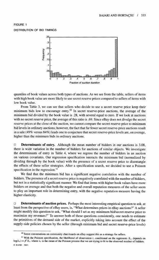
For each auction in our dataset, we collected the "final bids" as reported on the "bid history page." These final bids correspond to the maximum willingness-to-pay expressed by each bidder through the proxy bidding system (except for the winning bidder, whose maximum willingness- to-pay is not displayed). We found the book values for the auctioned items in the November 1998 issue of Coins Magazine, which surveys prices from coin dealers and coin auctions around the United States.7 As reported in Table 1, the average book value of the coins is $50, with values ranging from $3 to $3,700, reflecting the wide dispersion of prices even within this relatively narrow section of the collectible coin market. We reviewed item descriptions to see if the seller reported anything missing or wrong with the item being sold. This investigation labelled 9.3% of the items with self-reported blemishes.
Sellers on eBay are differentiated by their feedback rating. For each completed auction, eBay allows both the seller and the winning bidder to rate one another in terms of reliability and timeliness in payment and delivery. The rating is in the form of a positive, negative, or neutral response. Next to each buyer's or seller's ID (which is usually a pseudonym or an e-mail address), the number of net positive responses is displayed. By clicking on the ID, bidders can view all of the seller's feedback, including all comments as well as statistics totalling the total number of positive, neutral, and negative comments.
In Table 1, we see that the average bidder has 41 overall feedback points and the average seller has 202 overall feedback points. Negative feedback points are very low compared to the positive feedback points of the sellers.8 Users of eBay ascribe this to fear of retaliation, since the identities of feedback givers are displayed. Therefore, the conventional wisdom among eBay users is that the negative rating is a better indicator of a seller's reliability than her overall rating.
5 There were a total of 516 auctions completed in the mint/proof category during the five-day sample we considered. Bid histories for 39 auctions were lost due to a technical error in data transfer. Our dataset of 407 auctions represents all mint/proof set auctions conducted on eBay during the dates considered that had reliable book values and that were not Dutch auctions.
6 Mint sets contain uncirculated specimens of each year's coins for every denomination issued from each mint. Proof sets also contain a specimen of each year's newly minted coins, but are specially manufactured to have sharper details and more-than-ordinary brilliance compared to mint sets.
7 The November issue of the magazine was bought on October 22. The prices quoted were market prices as of mid-October.
8 The maximum negative rating of 21 corresponds to a seller with 973 overall feedback points. eBay discontinues a user's membership if the net of positive and negative feedback points falls below -4. ? RAND 2003.
332 / THE RAND JOURNAL OF ECONOMICS
TABLE 1 Summary Statistics
Standard Variable Mean Deviation Minimum Maximum
Book Value $50.1 $212.63 $3 $3700
Highest Bid/Book Value .81 .43 0 2.08
Winning Bid/Book Value (Conditional on Sale) .96 .30 .16 2.08
% Sold .79
Shipping and Handling $2.15 $1.02 $1 $5
% Blemished .09-
Number of Bidders 3.08 2.51 0 14
Minimum Bid//Book Value .63 .41 .0 2.56
% Secret Reserve .14
Seller's Overall Feedback 201.7 213.18 0 973
Seller's Negative Feedback .47 1.71 0 21
Bidder's Overall Feedback 41.2 37.54 -4 199.67
The average bidder and seller in this market has a reasonably high number of overall feedback
points, indicating that they can be classified as a serious collector, or possibly a coin dealer.
3. Some empirical regularities * In this section we report several empirical regularities we have found about bidding behavior on eBay. We will use these regularities to motivate our structural model of bidding in eBay auctions.
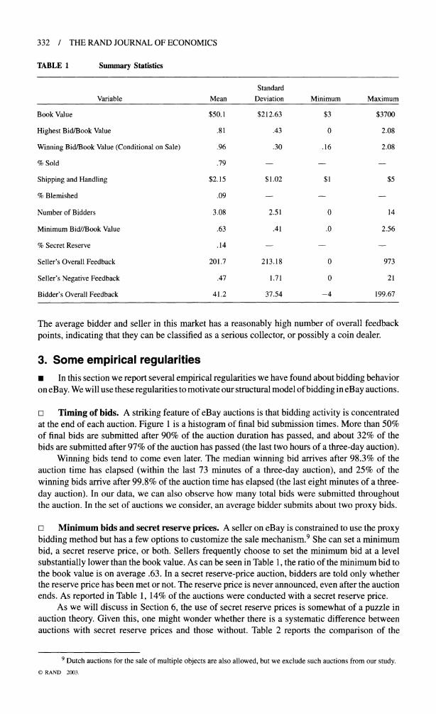
a Timing of bids. A striking feature of eBay auctions is that bidding activity is concentrated at the end of each auction. Figure 1 is a histogram of final bid submission times. More than 50% of final bids are submitted after 90% of the auction duration has passed, and about 32% of the bids are submitted after 97% of the auction has passed (the last two hours of a three-day auction).
Winning bids tend to come even later. The median winning bid arrives after 98.3% of the auction time has elapsed (within the last 73 minutes of a three-day auction), and 25% of the
winning bids arrive after 99.8% of the auction time has elapsed (the last eight minutes of a three-
day auction). In our data, we can also observe how many total bids were submitted throughout the auction. In the set of auctions we consider, an average bidder submits about two proxy bids.
z Minimum bids and secret reserve prices. A seller on eBay is constrained to use the proxy bidding method but has a few options to customize the sale mechanism.9 She can set a minimum bid, a secret reserve price, or both. Sellers frequently choose to set the minimum bid at a level substantially lower than the book value. As can be seen in Table 1, the ratio of the minimum bid to the book value is on average .63. In a secret reserve-price auction, bidders are told only whether the reserve price has been met or not. The reserve price is never announced, even after the auction ends. As reported in Table 1, 14% of the auctions were conducted with a secret reserve price.
As we will discuss in Section 6, the use of secret reserve prices is somewhat of a puzzle in auction theory. Given this, one might wonder whether there is a systematic difference between auctions with secret reserve prices and those without. Table 2 reports the comparison of the
9 Dutch auctions for the sale of multiple objects are also allowed, but we exclude such auctions from our study. ? RAND 2003.
BAJARI AND HORTACSU / 333
FIGURE 1
DISTRIBUTION OF BID TIMINGS
.35
.3
.25 C(
iu .15-
.1-
.05
0 .1 .2 .3 .4 .5 .6 .7 .8 .9 1 Fraction of auction duration
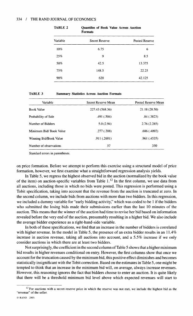
quantiles of book values across both types of auctions. As we see from the table, sellers of items with high book value are more likely to use secret reserve prices compared to sellers of items with low book value.
From Table 3, we can see that sellers who decide to use a secret reserve price keep their minimum bids low to encourage entry.10 In secret reserve-price auctions, the average of the minimum bid divided by the book value is .28, with several equal to zero. If we look at auctions with no secret reserve price, the average of this ratio is .69. Since eBay does not divulge the secret reserve prices at the close of the auction, we cannot compare the secret reserve price to minimum bid levels in ordinary auctions; however, the fact that far fewer secret reserve-price auctions result in a sale (49% versus 84%) leads one to conjecture that secret reserve-price levels are, on average, higher than the minimum bids in ordinary auctions.
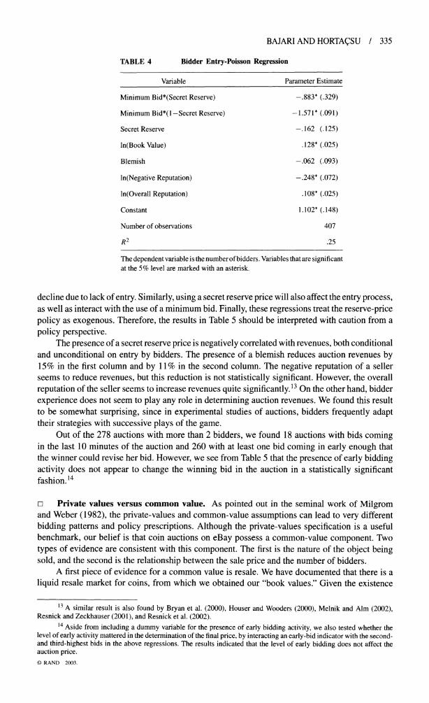
] Determinants of entry. Although the mean number of bidders in our auctions is 3.08, there is wide variation in the number of bidders for auctions of similar objects. We investigate the determinants of entry in Table 4, where we regress the number of bidders in an auction on various covariates. Our regression specification interacts the minimum bid (normalized by dividing through by the book value) with the presence of a secret reserve price to disentangle the effects of these seller strategies. After a specification search, we decided to use a Poisson specification in the regression.1I
We find that the minimum bid has a significant negative correlation with the number of bidders. The presence of a secret reserve price is negatively correlated with the number of bidders, but not in a statistically significant manner. We find that items with higher book values have more bidders on average and that both the negative and overall reputation measures of the seller seem to play an important role in determining entry, with the negative reputation measure having the higher elasticity.
D Determinants of auction prices. Perhaps the most interesting empirical question to ask, at least from the perspective of eBay users, is, "What determines prices in eBay auctions?" A seller might modify this question to ask, "What should I set as my minimum bid/secret reserve price to maximize my revenues?" To answer both of these questions consistently, one needs to estimate the primitives of the demand side of the market, explicitly taking into account the effect of the supply-side policies chosen by the seller (through minimum bid and secret reserve-price levels)
10 Some conversations on community chat-boards on eBay suggest this as a strategy for sellers. 11 With the Poisson specification, the likelihood of observation t, conditional on the regressors Xt, depends on
log(.t) = fi'Xt, where it is the mean of the Poisson process that we are trying to fit to the observed number of bidders. ? RAND 2003.
334 / THE RAND JOURNAL OF ECONOMICS
TABLE 2 Quantiles of Book Value Across Auction Formats
Variable Secret Reserve Posted Reserve
10% 6.75 6
25% 9 8.5
50% 42.5 13.375
75% 148.5 22.25
90% 620 42.125
TABLE 3 Summary Statistics Across Auction Formats
Variable Secret Reserve Mean Posted Reserve Mean
Book Value 227.43 (568.36) 21.18 (28.50)
Probability of Sale .491 (.504) .84 (.3823)
Number of Bidders 5.0 (2.94) 2.76 (2.285)
Minimum Bid/ Book Value .277 (.208) .686 (.4092)
Winning Bid/Book Value .911 (.2601) .961 (.4535)
Number of observations 57 350
Standard errors in parentheses.
on price formation. Before we attempt to perform this exercise using a structural model of price formation, however, we first examine what a straightforward regression analysis yields.
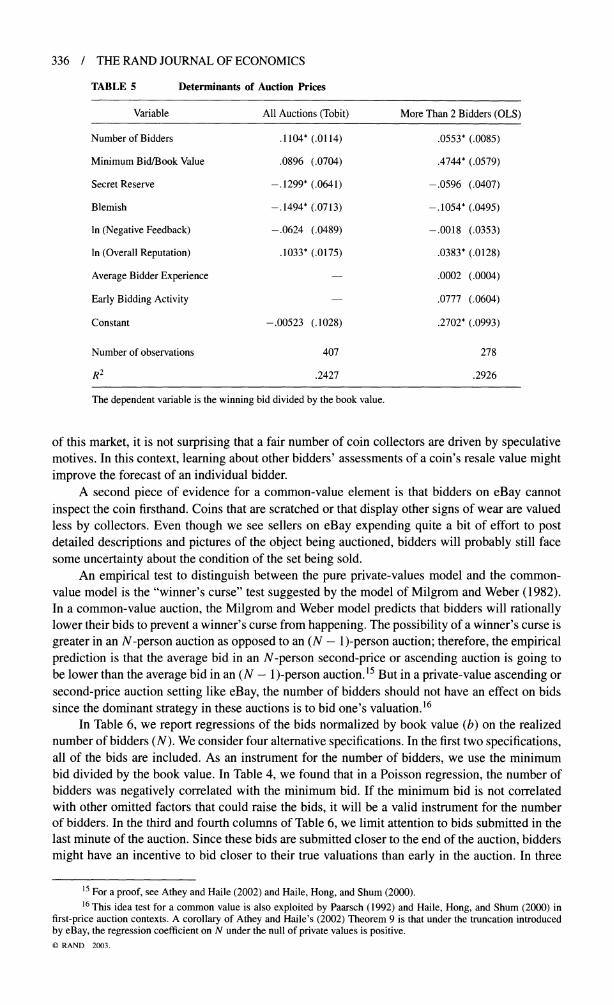
In Table 5, we regress the highest observed bid in the auction (normalized by the book value of the item) on auction-specific variables from Table 1.12 In the first column, we use data from all auctions, including those in which no bids were posted. This regression is performed using a Tobit specification, taking into account that the revenue from the auction is truncated at zero. In the second column, we include bids from auctions with more than two bidders. In this regression, we included a dummy variable for "early bidding activity," which was coded to be 1 if the bidders who submitted the losing bids made their submissions earlier than the last 10 minutes of the auction. This means that the winner of the auction had time to revise her bid based on information revealed before the very end of the auction, presumably resulting in a higher bid. We also include the average bidder experience as a right-hand-side variable.
In both of these specifications, we find that an increase in the number of bidders is correlated with higher revenue. In the model in Table 5, the presence of an extra bidder results in an 11.4% increase in auction revenue, taking all auctions into account, and a 5.5% increase if we only consider auctions in which there are at least two bidders.
Not surprisingly, the coefficient in the second column of Table 5 shows that a higher minimum bid results in higher revenues conditional on entry. However, the first columns show that once we account for the truncation caused by the minimum bid, this positive effect diminishes and becomes statistically insignificant with the Tobit correction. Based on the estimates in Table 5, one might be tempted to think that an increase in the minimum bid will, on average, always increase revenues. However, this reasoning ignores the fact that bidders choose to enter an auction. It is quite likely that there will be a threshold minimum bid level above which expected revenues will start to
12 For auctions with a secret reserve price in which the reserve was not met, we include the highest bid as the "revenue" of the seller. ? RAND 2003.
BAJARI AND HORTACSU / 335
TABLE 4 Bidder Entry-Poisson Regression
Variable Parameter Estimate
Minimum Bid*(Secret Reserve) -.883* (.329)
Minimum Bid*(1-Secret Reserve) -1.571* (.091)
Secret Reserve -.162 (.125)
ln(Book Value) .128* (.025)
Blemish -.062 (.093)
ln(Negative Reputation) -.248* (.072)
ln(Overall Reputation) .108* (.025)
Constant 1.102* (.148)
Number of observations 407
R2 .25
The dependent variable is the number of bidders. Variables that are significant at the 5% level are marked with an asterisk.
decline due to lack of entry. Similarly, using a secret reserve price will also affect the entry process, as well as interact with the use of a minimum bid. Finally, these regressions treat the reserve-price policy as exogenous. Therefore, the results in Table 5 should be interpreted with caution from a
policy perspective. The presence of a secret reserve price is negatively correlated with revenues, both conditional
and unconditional on entry by bidders. The presence of a blemish reduces auction revenues by 15% in the first column and by 11% in the second column. The negative reputation of a seller seems to reduce revenues, but this reduction is not statistically significant. However, the overall
reputation of the seller seems to increase revenues quite significantly.13 On the other hand, bidder
experience does not seem to play any role in determining auction revenues. We found this result to be somewhat surprising, since in experimental studies of auctions, bidders frequently adapt their strategies with successive plays of the game.
Out of the 278 auctions with more than 2 bidders, we found 18 auctions with bids coming in the last 10 minutes of the auction and 260 with at least one bid coming in early enough that the winner could revise her bid. However, we see from Table 5 that the presence of early bidding activity does not appear to change the winning bid in the auction in a statistically significant fashion. 14
o Private values versus common value. As pointed out in the seminal work of Milgrom and Weber (1982), the private-values and common-value assumptions can lead to very different
bidding patterns and policy prescriptions. Although the private-values specification is a useful benchmark, our belief is that coin auctions on eBay possess a common-value component. Two
types of evidence are consistent with this component. The first is the nature of the object being sold, and the second is the relationship between the sale price and the number of bidders.
A first piece of evidence for a common value is resale. We have documented that there is a
liquid resale market for coins, from which we obtained our "book values." Given the existence
13 A similar result is also found by Bryan et al. (2000), Houser and Wooders (2000), Melnik and Aim (2002), Resnick and Zeckhauser (2001), and Resnick et al. (2002).
14 Aside from including a dummy variable for the presence of early bidding activity, we also tested whether the level of early activity mattered in the determination of the final price, by interacting an early-bid indicator with the second- and third-highest bids in the above regressions. The results indicated that the level of early bidding does not affect the auction price. ? RAND 2003.
336 / THE RAND JOURNAL OF ECONOMICS
TABLE 5 Determinants of Auction Prices
Variable All Auctions (Tobit) More Than 2 Bidders (OLS)
Number of Bidders .1104* (.0114) .0553* (.0085)
Minimum Bid/Book Value .0896 (.0704) .4744* (.0579)
Secret Reserve -.1299* (.0641) -.0596 (.0407)
Blemish -.1494* (.0713) -.1054* (.0495)
In (Negative Feedback) -.0624 (.0489) -.0018 (.0353)
In (Overall Reputation) .1033* (.0175) .0383* (.0128)
Average Bidder Experience .0002 (.0004)
Early Bidding Activity -.0777 (.0604)
Constant -.00523 (.1028) .2702* (.0993)
Number of observations 407 278
R2 .2427 .2926
The dependent variable is the winning bid divided by the book value.
of this market, it is not surprising that a fair number of coin collectors are driven by speculative motives. In this context, learning about other bidders' assessments of a coin's resale value might improve the forecast of an individual bidder.
A second piece of evidence for a common-value element is that bidders on eBay cannot
inspect the coin firsthand. Coins that are scratched or that display other signs of wear are valued less by collectors. Even though we see sellers on eBay expending quite a bit of effort to post detailed descriptions and pictures of the object being auctioned, bidders will probably still face some uncertainty about the condition of the set being sold.
An empirical test to distinguish between the pure private-values model and the common- value model is the "winner's curse" test suggested by the model of Milgrom and Weber (1982). In a common-value auction, the Milgrom and Weber model predicts that bidders will rationally lower their bids to prevent a winner's curse from happening. The possibility of a winner's curse is
greater in an N-person auction as opposed to an (N - 1)-person auction; therefore, the empirical prediction is that the average bid in an N-person second-price or ascending auction is going to be lower than the average bid in an (N - 1)-person auction.15 But in a private-value ascending or
second-price auction setting like eBay, the number of bidders should not have an effect on bids since the dominant strategy in these auctions is to bid one's valuation.16
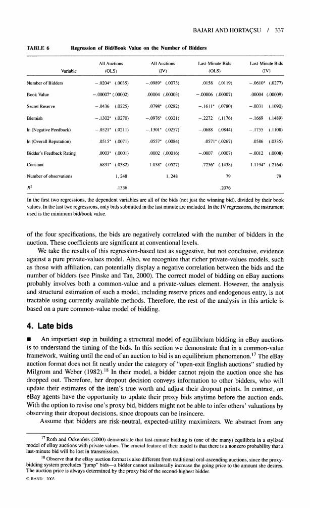
In Table 6, we report regressions of the bids normalized by book value (b) on the realized number of bidders (N). We consider four alternative specifications. In the first two specifications, all of the bids are included. As an instrument for the number of bidders, we use the minimum bid divided by the book value. In Table 4, we found that in a Poisson regression, the number of bidders was negatively correlated with the minimum bid. If the minimum bid is not correlated with other omitted factors that could raise the bids, it will be a valid instrument for the number of bidders. In the third and fourth columns of Table 6, we limit attention to bids submitted in the last minute of the auction. Since these bids are submitted closer to the end of the auction, bidders might have an incentive to bid closer to their true valuations than early in the auction. In three
15 For a proof, see Athey and Haile (2002) and Haile, Hong, and Shum (2000). 16 This idea test for a common value is also exploited by Paarsch (1992) and Haile, Hong, and Shum (2000) in
first-price auction contexts. A corollary of Athey and Haile's (2002) Theorem 9 is that under the truncation introduced by eBay, the regression coefficient on N under the null of private values is positive. ? RAND 2003.
BAJARI AND HORTA.SU / 337
TABLE 6 Regression of Bid/Book Value on the Number of Bidders
All Auctions All Auctions Last-Minute Bids Last-Minute Bids
Variable (OLS) (IV) (OLS) (IV)
Number of Bidders -.0204* (.0035) -.0989* (.0073) .0158 (.0119) -.0610* (.0277)
Book Value -.00007* (.00002) .00004 (.00003) -.00006 (.00007) .00004 (.00009)
Secret Reserve -.0436 (.0225) .0798* (.0282) -.1611' (.0780) -.0031 (.1090)
Blemish -.1302' (.0270) -.0976* (.0321) -.2272 (.1176) -.1669 (.1489)
In (Negative Feedback) -.0521' (.0211) -.1301' (.0257) -.0688 (.0844) -.1755 (.1108)
In (Overall Reputation) .0515* (.0071) .0557* (.0084) .0571* (.0267) .0586 (.0335)
Bidder's Feedback Rating .0003* (.0001) .0002 (.00016) -.0007 (.0007) -.0012 (.0008)
Constant .6831* (.0382) 1.038* (.0527) .7256* (.1438) 1.1194* (.2164)
Number of observations 1,248 1,248 79 79
R2 .1336 .2076
In the first two regressions, the dependent variables are all of the bids (not just the winning bid), divided by their book values. In the last two regressions, only bids submitted in the last minute are included. In the IV regressions, the instrument used is the minimum bid/book value.
of the four specifications, the bids are negatively correlated with the number of bidders in the auction. These coefficients are significant at conventional levels.
We take the results of this regression-based test as suggestive, but not conclusive, evidence against a pure private-values model. Also, we recognize that richer private-values models, such as those with affiliation, can potentially display a negative correlation between the bids and the number of bidders (see Pinske and Tan, 2000). The correct model of bidding on eBay auctions probably involves both a common-value and a private-values element. However, the analysis and structural estimation of such a model, including reserve prices and endogenous entry, is not tractable using currently available methods. Therefore, the rest of the analysis in this article is based on a pure common-value model of bidding.
4. Late bids * An important step in building a structural model of equilibrium bidding in eBay auctions is to understand the timing of the bids. In this section we demonstrate that in a common-value framework, waiting until the end of an auction to bid is an equilibrium phenomenon.17 The eBay auction format does not fit neatly under the category of "open-exit English auctions" studied by Milgrom and Weber (1982).18 In their model, a bidder cannot rejoin the auction once she has dropped out. Therefore, her dropout decision conveys information to other bidders, who will update their estimates of the item's true worth and adjust their dropout points. In contrast, on eBay agents have the opportunity to update their proxy bids anytime before the auction ends. With the option to revise one's proxy bid, bidders might not be able to infer others' valuations by observing their dropout decisions, since dropouts can be insincere.
Assume that bidders are risk-neutral, expected-utility maximizers. We abstract from any
17 Roth and Ockenfels (2000) demonstrate that last-minute bidding is (one of the many) equilibria in a stylized model of eBay auctions with private values. The crucial feature of their model is that there is a nonzero probability that a last-minute bid will be lost in transmission.
18 Observe that the eBay auction format is also different from traditional oral-ascending auctions, since the proxy- bidding system precludes "jump" bids-a bidder cannot unilaterally increase the going price to the amount she desires. The auction price is always determined by the proxy bid of the second-highest bidder. ? RAND 2003.
338 / THE RAND JOURNAL OF ECONOMICS
cross-auction considerations that bidders might have, and model strategic behavior in each auction as being independent from other auctions.19 Given our observation that there is not a big difference in bid levels across bidders with different feedback points, we assume that bidders are ex ante symmetric.
The informational setup of the game takes the following familiar form: let vi be the utility that bidder i gains from winning the auction, and let xi be her private information on the value of the object. We use the symmetric common value model of Wilson (1977), in which vi = v is a random variable whose realization is not observed until after the auction. In this model, private information for the bidder is xi = v + ?i, where Ei are i.i.d. Suppose that the minimum bid is zero and that there is no secret reserve.
Let us view the eBay auction as a two-stage auction. Taking the total auction time to be T, let the first-stage auction be an open-exit ascending auction played until T - e, where e << T is the time frame in which bidders on eBay cannot update their bids in response to others. The dropout points in this auction are openly observed by all bidders, who will be ordered by their dropout points in the first-stage auction, 01 < 02 < ... < On, with only On unobservable (bidders can only infer that it is higher than On- ). The second stage of the auction transpires from T - e to T and is conducted as a sealed-bid second-price auction. In this stage, every bidder, including those who dropped out in the first stage, is given the option to submit a bid, b. The highest bidder in the second-stage auction wins the object.
Given the above setup, we make the following claim:
Proposition 1. Bidding zero (or not bidding at all) in the first stage of the auction and participating only in the second stage of the auction is a symmetric Nash equilibrium of the eBay auction. In this case the eBay auction is equivalent to a sealed-bid second-price auction.
This result is based on the following lemma, whose proof is in the Appendix:
Lemma 1. The first-stage dropout points Oi, i = 1, ..., n cannot be of the form 0(xi), a monotonic function in bidder i's signal.
This lemma leads to the conclusion that the eBay auction format generates less information revelation during the course of the auction than in the Milgrom and Weber (1982) model of ascending auctions.
If we take the extreme case in which nobody bids in the first stage of the auction (or everybody bids zero), the second stage becomes a sealed-bid second-price auction, where each bidder knows only her own signal. In this case, the symmetric equilibrium bid function, as derived by Milgrom and Weber, will be b(x) = v(x, x), where v(x, y) = E[v xi = x, Yi = y], with yi = maxjy{1....n}{\ i xj}.20
5. A structural model of eBay auctions * In this section we specify a structural econometric model of eBay auctions. The structural parameters we estimate are the distribution of bidder's private information and a set of parameters that govern entry into the auction. Estimates of the structural parameters allow us to better understand the determinants of bidder behavior. Also, the structural parameters can be used to simulate the magnitude of the winner's curse in this market and the impact of different
19 We recognize that similar objects are often being sold side by side on eBay and that bidding strategies could be different in this situation. We believe that investigating such strategies is an interesting avenue of future research; however, for the sake of tractability, we have chosen to ignore this aspect of bidding. We recognize, however, that this feature of eBay auctions might play a role in explaining late bidding.
20 To rule out profitable deviations, observe the following: if bidder j were to unilaterally deviate from the proposed equilibrium of not bidding at all in the first stage, then the proxy-bidding system of eBay would indicate that this bidder's signal xj is greater than zero and not much else, since bidder j's bid would advance the "maximum bid" to one increment above zero; therefore bidder j would not be able to signal or "scare" away competition. Further, since signals are affiliated, E[v I xi = x, yi = x, xj > 0] > E[v I xi = x, Yi = x], so bidder j would unilaterally decrease her probability of winning. ? RAND 2003.

BAJARI AND HORTACSU / 339
reserve prices on seller revenue. Motivated by the results of the previous sections, we model an eBay auction as a second-price sealed-bid auction where the number of bidders is endogenously determined by a zero-profit condition in a manner similar to Levin and Smith (1994).21 Assume there are N potential bidders viewing a particular listing on eBay. However, not every potential bidder enters the auction, since each entering bidder has to bear a bid-preparation cost, c. In the context of eBay, c represents the cost of the effort spent on estimating the value of the coin and the opportunity cost of time spent bidding. After paying c, a bidder receives her private signal, xi, of the common value of the object, v. Like Levin and Smith (1994), our analysis focuses on the symmetric equilibrium of the endogenous-entry game, in which each bidder enters the auction with an identical entry probability, p. In equilibrium, entry will occur until each bidder's ex ante expected profit from entering the auction is zero.
Let Vn be the ex ante expected value of the item when it is common knowledge that there are n bidders in the auction. Let Wn be the ex ante expected payment the winning bidder will make to the seller when there are n bidders. Since bidders are ex ante symmetric, a bidder's ex ante expected profit, conditional on entering an auction with n bidders, will be equal to (Vn - Wn)/n-c. The seller can set a minimum bid, which we denote by r. Define Tn(r) to be the probability of trade given n and a minimum bid r. Given these primitives, the following zero-profit condition will hold in equilibrium:
Np T , (Vn Wn)( c= pTnin(r) (1)
In equation (1), is the probability that there are n bidders in the auction, conditional on entry In equation (1), p/ is the probability that there are n bidders in the auction, conditional on entry by bidder i.
As in Levin and Smith (1994), we assume that the unconditional distribution of bidders within an auction is binomial, with each of the N potential bidders entering the auction with probability p. On eBay, the potential number of bidders is likely to be quite large compared to the actual number of bidders. Therefore, we will use the Poisson approximation to the binomial distribution. With the Poisson approximation, the probability that there are n bidders in the auction, conditional on bidder i's presence, is p = e-~X.n-1/(n- )!,n = 1,... oc, where = E[n] = Np. The mean of the Poisson entry process, ., will be determined endogenously by the zero-profit condition (1). In equilibrium, X is assumed to be common knowledge.
Conditional on entry, we will assume that the bidders will play the "last-minute bidding" equilibrium of the game derived in the previous section. However, bidders do not observe n, the actual number of competitors, when submitting their bids. Therefore, by the results in Section 4, the equilibrium bidding strategies are equivalent to a second-price sealed-bid auction with a stochastic number of bidders. We also allow the sellers to use a secret reserve price. To abstract from any strategic concerns from the seller's side and to make structural estimation tractable, we assume that the bidders believe that the seller's estimate of the common value comes from the same distribution as the bidders' estimates.22 Given a signal x, we assume that the seller sets a secret reserve price using the same bid function as the bidders in the auction. Therefore, from the bidders' perspective, the seller is just another bidder. With this assumption, the only difference between the secret reserve-price auction and a regular auction is that now all potential bidders know that they face at least one competitor-the seller. Following Milgrom and Weber, define yn) = maxjy{l ...n}\i {xj } to be the maximum estimate of the n bidders, excluding bidder i. Let
21 We acknowledge that this equilibrium does not entirely fit the observed bidding behavior on eBay; as Figure 2 displays, not all of the bids arrive during the last 5 to 10 minutes of the auction. However, our finding in Section 3 that early-bidding activity does not affect the winning bid is consistent with Lemma 1: early bids cannot be taken seriously in the "second stage" if bidders can jump in at the last second.
22 This strategy is optimal for the seller if his valuation for the item is the same as the bidders' and the last-minute bidding equilibrium is used. We recognize, however, that it is not clear whether it is rational for the seller to put the item up for sale in this environment. However, in order to specify the likelihood function, the model must account for bidders' beliefs about the distribution of the reserve price. ? RAND 2003.
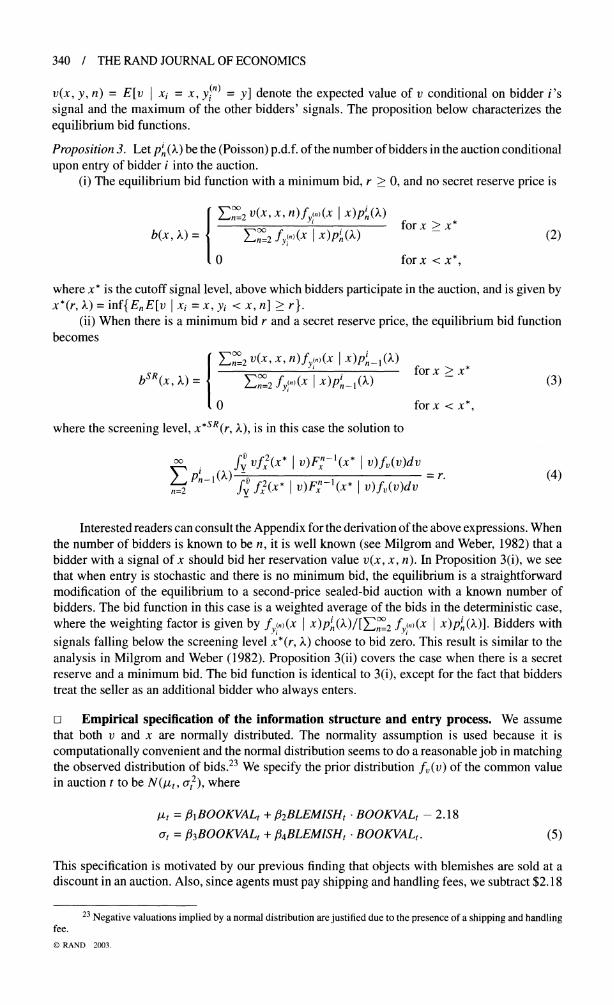
340 / THE RAND JOURNAL OF ECONOMICS
v(x, y, n) = E[v I xi = x, y(n) = y] denote the expected value of v conditional on bidder i's signal and the maximum of the other bidders' signals. The proposition below characterizes the equilibrium bid functions.
Proposition 3. Let p/ (X) be the (Poisson) p.d.f. of the number of bidders in the auction conditional upon entry of bidder i into the auction.
(i) The equilibrium bid function with a minimum bid, r > 0, and no secret reserve price is
E00=2 (X, X, n)fy ()(X I x)pi () Eb(x , A) =
I n =2o f, ( )nX j Px p.l t ) for x > x *
b(x, ) = f n (2)
0 forx <x*,
where x* is the cutoff signal level, above which bidders participate in the auction, and is given by x*(r, )) = inf{EnE[v I xi = x, Yi < x, n] > r}.
(ii) When there is a minimum bid r and a secret reserve price, the equilibrium bid function becomes
n=2 v(X, , n)f(n | x)pX (i ) fo > O for x > x*
bSR(x, ) = . Yn=2 fn)fyx\(x)p I
i- (3)
0 forX < *,
where the screening level, x*SR(r, X), is in this case the solution to
? fvv vfx2(x* I v)Fxn-(x* I v)fv(v)dv >3pn1(X '- =r. (4)
n=2 iKv f 2(x* v)Fxn- (* v)fv(v)dv
Interested readers can consult the Appendix for the derivation of the above expressions. When the number of bidders is known to be n, it is well known (see Milgrom and Weber, 1982) that a bidder with a signal of x should bid her reservation value v(x, x, n). In Proposition 3(i), we see that when entry is stochastic and there is no minimum bid, the equilibrium is a straightforward modification of the equilibrium to a second-price sealed-bid auction with a known number of bidders. The bid function in this case is a weighted average of the bids in the deterministic case, where the weighting factor is given by fy(n)(X I )pI(X)/[Pni =2 fy()(x x)p '()]. Bidders with
signals falling below the screening level x*(r, X) choose to bid zero. This result is similar to the analysis in Milgrom and Weber (1982). Proposition 3(ii) covers the case when there is a secret reserve and a minimum bid. The bid function is identical to 3(i), except for the fact that bidders treat the seller as an additional bidder who always enters.
] Empirical specification of the information structure and entry process. We assume that both v and x are normally distributed. The normality assumption is used because it is computationally convenient and the normal distribution seems to do a reasonable job in matching the observed distribution of bids.23 We specify the prior distribution fv(v) of the common value in auction t to be N(,tt, ct2), where
ltt = ,B1BOOKVALt + B2BLEMISHt ? BOOKVALt - 2.18
at = B3BOOKVALt + /4BLEMISHt ? BOOKVALt. (5)
This specification is motivated by our previous finding that objects with blemishes are sold at a discount in an auction. Also, since agents must pay shipping and handling fees, we subtract $2.18
23 Negative valuations implied by a normal distribution are justified due to the presence of a shipping and handling fee. ? RAND 2003.
BAJARI AND HORTACSU / 341
in computing tt, the average shipping and handling fee for the mint/proof sets.24 We assume that the distribution of individual signals fx(x I v) conditional on the common value v is N(vt, kt2), where k = P5 is a parameter to be estimated.
The zero-profit condition (1) suggests that in our estimation procedure, we should treat the entry cost, c, as an exogenous parameter and endogenously derive the equilibrium distribution of entrants as characterized by Xt. This is a computationally intractable problem. Solving for it requires that we find the solution to a nonlinear equation, which can only be evaluated ap- proximately because the expectation terms involve multidimensional integrals. Instead, motivated by the regression in Table 4, we use the following reduced-form specification for it:
log it = P6 + /7SECRETt + f8LN(BOOKt) + B9NEGATIVEt MINBIDt MINBIDt + fBloSECRETt BOOKAL + Ill(l - SECRETt)BOOKVAL. (6)
BOOKVALt BOOKVALt
In equation (6), the entry probability depends on the book value, the seller's negative feedback, and the reserve price. Our reduced-form specification for it is consistent with equations (1) and (5), since these equations imply that the distribution of entrants should be a function of the book value, the dummy for a blemish, and the reserve price used by the seller.
E Estimation. The model outlined in the previous subsection generates a likelihood function in a natural way. Let Q2t = {SECRETt, rt}, t = (1, ..., pfl) and
Zt = (BOOKVALt, BLEMISHt, NEGATIVEt).
Let b(x I| t, f, Zt) be the equilibrium bid function conditional on Qt, the structural parameters 8, and the set of covariates Zt. Since bids are strictly increasing in x, an inverse bid function
exists, which we denote as (p(b Qt, 8, Zt). Let fb(bi I Qt, , Zt, v) denote the p.d.f. for the distribution of bids conditional on Qt, B, Zt, and the realization of the common value v. By a simple change of variables argument, fb must satisfy the equation below:
fb(bi I Qt, , Zt, v) = fx(((b I Qt, , Zt) I v, k, ot)t'(bi I Qt,, Zt). (7)
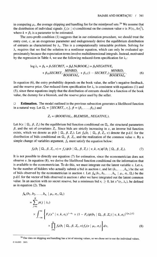
It is not possible to directly use equation (7) for estimation, since the econometrician does not observe v. In equation (8), we derive the likelihood function conditional on the information that is available to the econometrician. To do this, we must integrate out the latent variable v. Let nt be the number of bidders who actually submit a bid in auction t, and let (b, ..., bn,) be the set of bids observed by the econometrician in auction t. Let fb,(bl, b2, ..., bn, t, Ot, Q't, ) be the p.d.f. for the vector of bids observed in auction t after we have integrated out the latent common value. In an auction with no secret reserve, but a minimum bid rt > 0, let x*(rt, At), be defined as in equation (2). Then
fb, (bl, b2, . .. b bn, I| tt, Ot, Qt) N
= EP(j I )t)
x Fx(x* v, k, oat)j-n x (1 - Fx((b, Qt, Z) v, k, t)l{n>l J -oo
nt
x n fb(bi I Qt, B Zt, v)fv(v I Ilt, ort) d, (8) i=2
24 Our data on shipping and handling has a lot of missing values, so we chose not to use the individual values. ? RAND 2003.
342 / THE RAND JOURNAL OF ECONOMICS
where 1 {n > 1} is an indicator variable for the event that there is at least one bidder in the auction and N is an upper bound on the number of entrants.25 Observe that this specification allows us to assign a positive likelihood to auctions with no bidders. For auctions with a secret reserve price, the likelihood function in (8) is modified to reflect that bidders view the seller as another competitor (who is certain to be there), and as a result the bidders use a different bid function.
When computing these likelihood functions, the following result helps immensely in reducing the computational complexity of the estimation algorithm.
Proposition 4. Let b(x I ut?, a?, k, .) be the bid function in an auction where the common value, v, is distributed normally with mean ut? and standard deviation a?, generating signal x with mean v and variance k(? )2. If we change the scaling of the common value and signal distribution such that the scaled common value, v', is distributed with mean a1l /? + a2 and standard deviation a la?, and the scaled signal, x', is distributed with mean v' and variance k(al a?)2, the equilibrium bid
corresponding to the scaled signal, x', under the scaled signal and common-value distribution, can be calculated as aolb([x' - al]/Oa2 I i0, a?, k, X) + a2.
The Appendix contains a proof of Proposition 4. This is a key result in our estimation
procedure because it allows us to compute the bid function only once for a base-case auction. We can then apply an affine transformation to this "precomputed" function to find the bid function in an auction where the distribution of the common value has a different mean and variance.26
We use recently developed methods in Bayesian econometrics for estimation. We first specify a prior distribution for the parameters and then apply Bayes' theorem to study the properties of the posterior. We use Markov-chain Monte Carlo methods described in the Appendix to simulate the posterior distribution of the model parameters.
There are four advantages to a Bayesian approach when estimating parametric auction models. First, Bayesian methods are computationally simple, and we find these methods much easier to implement than maximum likelihood, which involves numerical optimization in several dimensions. Second, it is not possible to apply standard asymptotic theory in a straightforward manner in many auction models because the support of the distribution of bids depends on the parameters. Third, confidence intervals in a classical framework are commonly based on second-order asymptotic approximations. Our results are correct in finite samples and do not
require invoking the assumptions used in second-order asymptotics. Fourth, Porter and Hirano (2001) have found that in some parametric-auction models, Bayesian methods are asymptotically efficient while some commonly used classical methods are often not efficient. The details of how to compute our estimates can be found in the Appendix.27
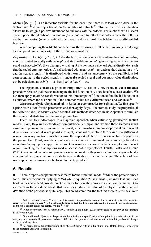
6. Results * Table 7 reports our parameter estimates for the structural model.28 Since the posterior mean for P1, the coefficient multiplying BOOKVAL in equation (5), is almost 1, we infer that published book values do indeed provide point estimates for how the coins are valued on the market. Our estimates in Table 7 demonstrate that blemishes reduce the value of the object, but the standard deviation of the posterior is quite large. This could stem from the fact that these "blemishes" were
25 With a Poisson process, N = oo. But this makes it impossible to account for the truncation in bids due to the reserve price, hence we take N to be sufficiently large so that the difference between the truncated Poisson distribution and the full distribution is negligible. We use N = 30.
26 Other researchers, such as Paarsch (1992) and Hong and Shum (2002), have exploited linearity of bid functions in different models.
27 One traditional objection to Bayesian methods is that the specification of the prior is typically ad hoc. In our analysis, there are only 11 parameters and over 1,000 bids. Our parameter estimates are therefore fairly robust to changes in the prior distribution.
28 All results are from a posterior simulation of 30,000 draws with an initial "bum-in" of 10,000 draws. Convergence to the posterior appeared to be rapid. ? RAND 2003.
BAJARI AND HORTAtSU / 343
TABLE 7 Posterior Means and Standard Deviations: Full Sample
Standard Parameter Variable Mean Deviation
-z BOOKVAL .9911 .0387
BOOKVAL * BLEMISH -.1446 .1628
a BOOKVAL .5599 .0260
BOOKVAL * BLEMISH .0326 .0260
k .2545 .0259
CONSTANT 1.4069 .0897
SECRET -.2857 .1080
X LN(BOOK) .0883 .0276
NEGATIVE -.0414 .0228
SECRET * (MINBID/BOOKVAL) -.2514 .3268
(1 - SECRET) * (MINBID/BOOKVAL) -.7893 .0864
coded by "noncollectors" who might have introduced noise into our coding. A $1 increase in BOOKVAL increases the posterior mean of oa by $.56. Therefore, a large amount of variation between the values of the different coins in our dataset is not captured by the book value and the presence of a blemish alone.
Our estimates imply that the standard deviation of the bidders' signals, xi, is only k/2a = 28.25% of the book value. Therefore, the bidders' signals of v are much more clustered than the unconditional distribution of v, suggesting that bidders are quite proficient in acquiring information about the items for sale.
The main determinants of entry are the reserve-price mechanism, the minimum bid level, and the book value of the coin. Negative seller reputation was found to reduce entry, while the minimum bid level in a secret reserve-price auction does not affect the entry decision significantly.
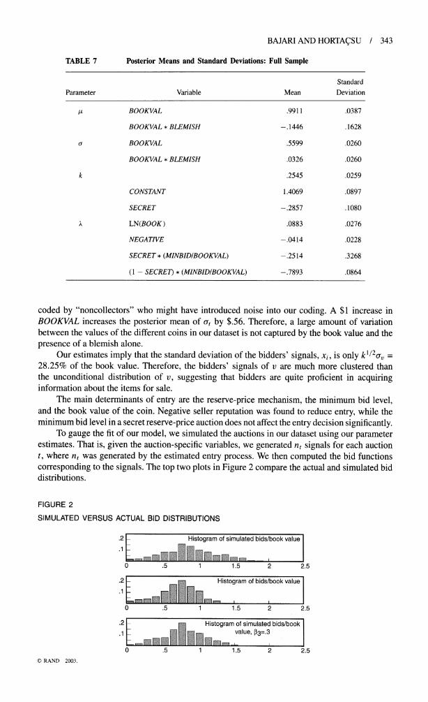
To gauge the fit of our model, we simulated the auctions in our dataset using our parameter estimates. That is, given the auction-specific variables, we generated nt signals for each auction t, where nt was generated by the estimated entry process. We then computed the bid functions corresponding to the signals. The top two plots in Figure 2 compare the actual and simulated bid distributions.
FIGURE 2
SIMULATED VERSUS ACTUAL BID DISTRIBUTIONS
.2 - Histogram of simulate
__ -
sd bids/book value
0 .5 1 1.5 2 2.5
.2 - Histogi
.1 I f l ram of bids/book value
I
0 .5 1 1.5 2 2.5
.2 - Histogram of simulated bids/book
.1 i^: 1 i g H value,l, 23=.3
0 .5 1 1.5 2 2.5 ? RAND 2003.
344 / THE RAND JOURNAL OF ECONOMICS
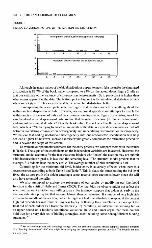
FIGURE 3
SIMULATED VERSUS ACTUAL WITHIN-AUCTION BID DISPERSION
.6 Histogram of within-auction bid dispersion: simulated
.4 -
.5 .1 .15 .2 .25 .3 .35 .4 .45 .5
.6 Histogram of within-auction bid dispersion: actual
.4
.2
0o F]r7m 5 .1 ,15 I n .25 .3 .5 m i,,M. r .4 .5 .1 .15 .2 .25 .3 .35 .4 .45 .5
Although the mean values of the bid distributions appear to match (the mean for the simulated distribution is 82.7% of the book value, compared to 83% for the actual data), Figure 2 tells us that our estimate of the variance of cross-auction heterogeneity (83 in particular) is higher than what seems apparent in the data. The bottom plot in Figure 2 is the simulated distribution of bids when we set B3 = .3. This seems to match the actual bid distribution better.
In interpreting the above plots, note that Figure 2 alone does not tell us anything about the within-auction dispersion of bids. However, our empirical specification attempts to match the within-auction dispersion of bids and the cross-auction dispersion. Figure 3 is a histogram of the simulated and actual dispersion of bids. We find that the mean dispersion (difference between max and min) of the simulated bids is 23% of the book value. This is lower than the actual dispersion of bids, which is 32%. In trying to match all moments of the data, our specification makes a tradeoff between overstating cross-auction heterogeneity and understating within-auction heterogeneity. We believe that adding unobserved heterogeneity into our econometric specification will help achieve a tighter fit; however, such an exercise would greatly complicate the estimation procedure and is beyond the scope of this article.
To evaluate our parameter estimates for the entry process, we compare them with the results in Table 4. The signs of the coefficients on the independent variables are in accord. However, the structural model accounts for the fact that some bidders who "enter" the auction may not submit a bid because their signal xi is less than the screening level. The structural model predicts that on average, 3.3 bidders bear the entry cost c. The average number of bids submitted is 3.01.
Controlling for the minimum bid level, bidder entry is adversely affected when there is a secret reserve, according to both Table 4 and Table 7. This is plausible, since holding the bid level fixed, the ex ante profit of a bidder entering a secret reserve-price auction is lower, since she will also have to outbid the seller.
We also attempted to explore the robustness of our results by modifying our likelihood function in the spirit of Haile and Tamer (2003). The final bids we observe might not reflect the maximum amount a bidder was willing to pay. For instance, suppose that bidder A, early in the auction, submits a proxy bid that was much lower than her valuation. If a number of very high bids arrive in the middle of the auction, bidder A might not find it worthwhile to respond if the current high bid exceeds her maximum willingness to pay. Following Haile and Tamer, we interpret the final bid of each bidder as a lower bound on v(x, x). Similarly, we interpret the winning bid as an upper bound on a bidder's conditional valuation. Haile and Tamer argue that these bounds hold true for a very rich set of bidding strategies, even including some nonequilibrium bidding strategies.29
29 We acknowledge that this bounding strategy does not take into account certain complex dynamic elements like "learning from others' bids" that might be underlying the data-generation process on eBay. The bounds are also ? RAND 2003.
BAJARI AND HORTACSU / 345
FIGURE 4
WINNER'S CURSE EFFECT
90 -Bid functions for the . . 80 - representative auction . 70 -- b(x)
- - - b(x) with an extra bidder .. 60 - - b(x) with sigma =.1 . : -
50 ....... b(x)= x
40 - 30 -
20 - -.5^ 10 ,-...
10 20 30 40 50 60 70 80 90 x- estimate ($)
The main difference resulting from the use of bounds in our likelihood function specifications decreased the parameter controlling the variance of the signal distribution (/83) to .28. As discussed above, this is an improvement over our previous estimates in terms of matching the across-auction dispersion of bids. However, this estimate predicts a much tighter distribution of bids within an auction (10% of book value) than is seen in the data-under the assumption that bidders play the equilibrium of the second-price auction game when forming the predicted distribution. This points out the main difficulty of applying a "bounds" approach in our setting: since the econometric specification does not specify an equilibrium model, even if structural parameters are estimated accurately, it is difficult to make in-sample or out-of-sample predictions-or to conduct policy simulations with the estimated model-unless the bounds used for estimation imply informative bounds on predicted equilibrium behavior or policy outcomes.30 Therefore, we elect to proceed with the parameter estimates in Table 7, which are generated by an empirical specification based on a fully specified equilibrium model of bidding. Nevertheless, we believe that further research in using a bounds approach is well warranted.
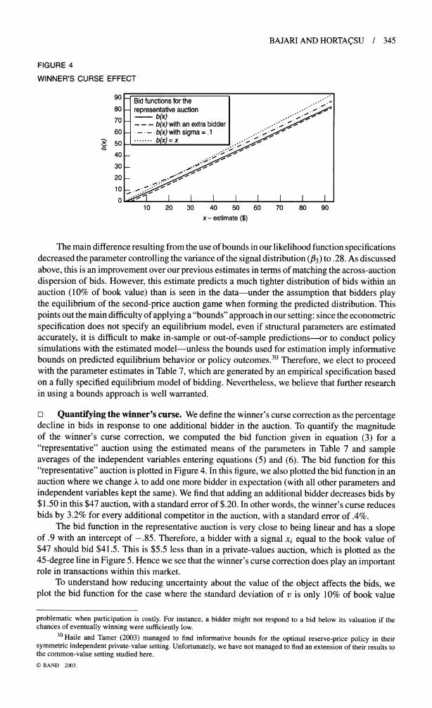
o Quantifying the winner's curse. We define the winner's curse correction as the percentage decline in bids in response to one additional bidder in the auction. To quantify the magnitude of the winner's curse correction, we computed the bid function given in equation (3) for a "representative" auction using the estimated means of the parameters in Table 7 and sample averages of the independent variables entering equations (5) and (6). The bid function for this "representative" auction is plotted in Figure 4. In this figure, we also plotted the bid function in an auction where we change X to add one more bidder in expectation (with all other parameters and independent variables kept the same). We find that adding an additional bidder decreases bids by $1.50 in this $47 auction, with a standard error of $.20. In other words, the winner's curse reduces bids by 3.2% for every additional competitor in the auction, with a standard error of .4%.
The bid function in the representative auction is very close to being linear and has a slope of .9 with an intercept of -.85. Therefore, a bidder with a signal xi equal to the book value of $47 should bid $41.5. This is $5.5 less than in a private-values auction, which is plotted as the 45-degree line in Figure 5. Hence we see that the winner's curse correction does play an important role in transactions within this market.
To understand how reducing uncertainty about the value of the object affects the bids, we plot the bid function for the case where the standard deviation of v is only 10% of book value
problematic when participation is costly. For instance, a bidder might not respond to a bid below its valuation if the chances of eventually winning were sufficiently low.
30 Haile and Tamer (2003) managed to find informative bounds for the optimal reserve-price policy in their symmetric independent private-value setting. Unfortunately, we have not managed to find an extension of their results to the common-value setting studied here. ? RAND 2003.
346 / THE RAND JOURNAL OF ECONOMICS
FIGURE 5
EXPECTED NUMBER OF BIDDERS AS A FUNCTION OF MINIMUM BID
4.5 4-
-o 3.5- e 3 -
) D 2.5 -
.5 -
0 I I I I
.2 .4 .6 .8 1 1.2 1.4 Minimum bid/book value
(as opposed to 52%). As expected, the bids increase: a bidder with a signal xi of $47 bids $45. Clearly, sellers can increase profits by reducing the bidders' uncertainty about the value of the coin set.31
m Quantifying the entry cost to an eBay auction. Our finding that the minimum bid plays an important role in determining entry into an auction naturally leads us to question the magnitude of the implicit entry costs faced by the bidders. We can estimate entry costs using the zero-profit condition, equation (1).
Using our parameter estimates, assuming that the item characteristics are from the "representative auction" used in the winner's curse calculation, we can calculate all of the terms on the right-hand side of equation (1). This allows us to infer the value of c. Using the simulation method described in Bajari and Hortacsu (2000), we find that the implied value of c is $3.20, with a standard error of $1.48.
The implied entry cost changes with auction characteristics. However, the entry cost as a percentage of the book value seems stable. For example, for an auction with book value $1,000 and a minimum bid of $600, the computed entry cost is $66.
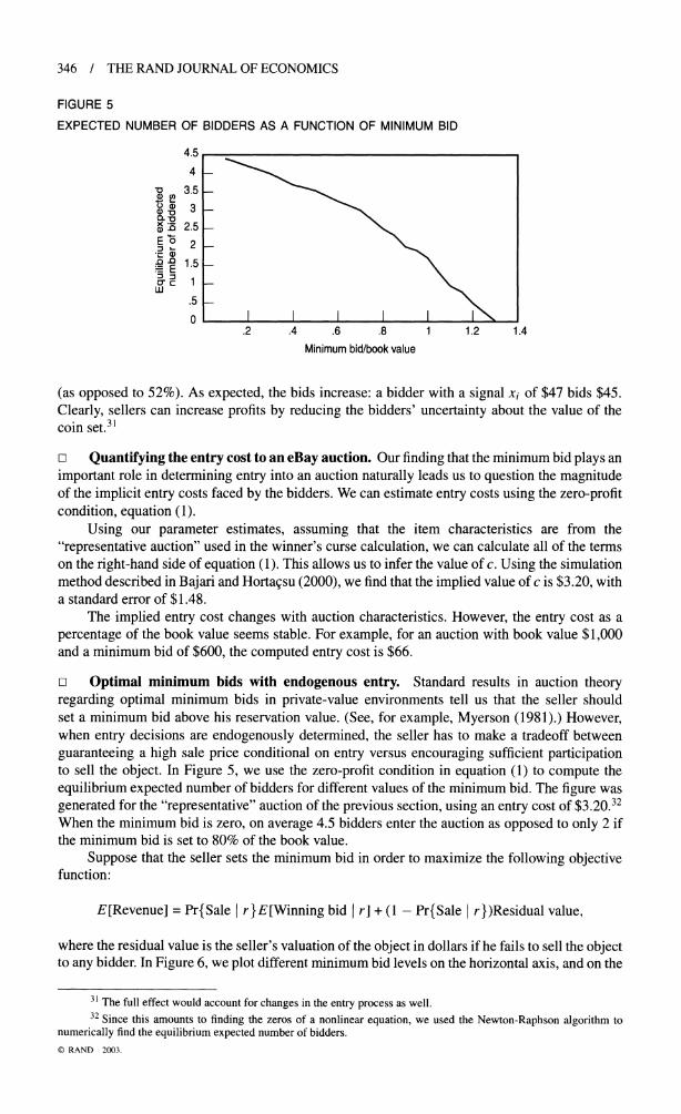
D Optimal minimum bids with endogenous entry. Standard results in auction theory regarding optimal minimum bids in private-value environments tell us that the seller should set a minimum bid above his reservation value. (See, for example, Myerson (1981).) However, when entry decisions are endogenously determined, the seller has to make a tradeoff between guaranteeing a high sale price conditional on entry versus encouraging sufficient participation to sell the object. In Figure 5, we use the zero-profit condition in equation (1) to compute the equilibrium expected number of bidders for different values of the minimum bid. The figure was generated for the "representative" auction of the previous section, using an entry cost of $3.20.32 When the minimum bid is zero, on average 4.5 bidders enter the auction as opposed to only 2 if the minimum bid is set to 80% of the book value.
Suppose that the seller sets the minimum bid in order to maximize the following objective function:
E[Revenue] = Pr{Sale } r}E[Winning bid I r] + (1 - Pr{Sale } r})Residual value,
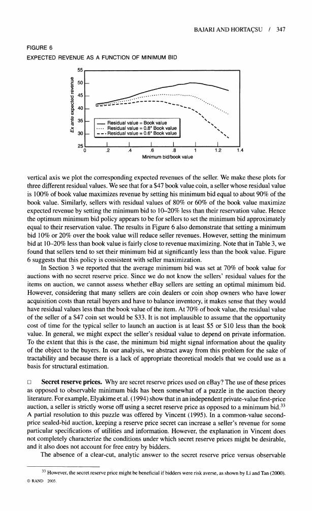
where the residual value is the seller's valuation of the object in dollars if he fails to sell the object to any bidder. In Figure 6, we plot different minimum bid levels on the horizontal axis, and on the
31 The full effect would account for changes in the entry process as well. 32 Since this amounts to finding the zeros of a nonlinear equation, we used the Newton-Raphson algorithm to
numerically find the equilibrium expected number of bidders. ? RAND 2003.
BAJARI AND HORTA(SU / 347
FIGURE 6
EXPECTED REVENUE AS A FUNCTION OF MINIMUM BID
55
a) 50 -
- ...................
c 35 - Residual value = Book value
25 1 1 1 0 .2 .4 .6 .8 1 1.2 1.4
Minimum bid/book value
vertical axis we plot the corresponding expected revenues of the seller. We make these plots for three different residual values. We see that for a $47 book value coin, a seller whose residual value is 100% of book value maximizes revenue by setting his minimum bid equal to about 90% of the book value. Similarly, sellers with residual values of 80% or 60% of the book value maximize
expected revenue by setting the minimum bid to 10-20% less than their reservation value. Hence the optimum minimum bid policy appears to be for sellers to set the minimum bid approximately equal to their reservation value. The results in Figure 6 also demonstrate that setting a minimum bid 10% or 20% over the book value will reduce seller revenues. However, setting the minimum bid at 10-20% less than book value is fairly close to revenue maximizing. Note that in Table 3, we found that sellers tend to set their minimum bid at significantly less than the book value. Figure 6 suggests that this policy is consistent with seller maximization.
In Section 3 we reported that the average minimum bid was set at 70% of book value for auctions with no secret reserve price. Since we do not know the sellers' residual values for the items on auction, we cannot assess whether eBay sellers are setting an optimal minimum bid. However, considering that many sellers are coin dealers or coin shop owners who have lower acquisition costs than retail buyers and have to balance inventory, it makes sense that they would have residual values less thant t he book valu e o item. At 70% of book value, the residual value of the seller of a $47 coin set would be $33. It is not implausible to assume that the opportunity cost of time for the typical seller to launch an auction is at least $5 or $10 less than the book value. In general, we might expect the seller's residual value to depend on private information. To the extent that this is the case, the minimum bid might signal information about the quality of the object to the buyers. In our analysis, we abstract away from this problem for the sake of tractability and because there is a lack of appropriate theoretical models that we could use as a basis for structural estimation.
o Secret reserve prices. Why are secret reserve prices used on eBay? The use of these prices as opposed to observable minimum bids has been somewhat of a puzzle in the auction theory literature. For example, Elyakime et al. (1994) show that in an independent private-value first-price auction, a seller is strictly worse off using a secret reserve price as opposed to a minimum bid.33 A partial resolution to this puzzle was offered by Vincent (1995). In a common-value second- price sealed-bid auction, keeping a reserve price secret can increase a seller's revenue for some particular specifications of utilities and information. However, the explanation in Vincent does not completely characterize the conditions under which secret reserve prices might be desirable, and it also does not account for free entry by bidders.
The absence of a clear-cut, analytic answer to the secret reserve price versus observable
33 However, the secret reserve price might be beneficial if bidders were risk averse, as shown by Li and Tan (2000). ? RAND 2003.
348 / THE RAND JOURNAL OF ECONOMICS
FIGURE 7
EXPECTED REVENUE DIFFERENCE BETWEEN SECRET AND POSTED MINIMUM BID POLICY
1.6
1.4-
D 1.2-
E 1-
I - .8-
.4 -
m .2 w
20 40 60 80 100 120 140 160 180 200 20 40 60 80 100 120 140 160 180 200 Book value ($)
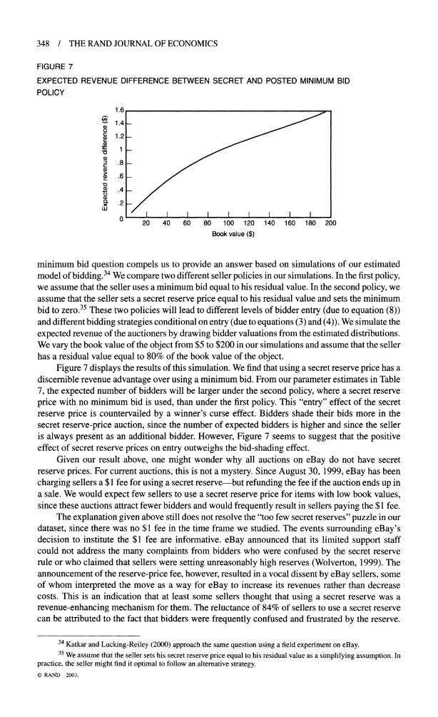
minimum bid question compels us to provide an answer based on simulations of our estimated model of bidding.34 We compare two different seller policies in our simulations. In the first policy, we assume that the seller uses a minimum bid equal to his residual value. In the second policy, we assume that the seller sets a secret reserve price equal to his residual value and sets the minimum bid to zero.35 These two policies will lead to different levels of bidder entry (due to equation (8)) and different bidding strategies conditional on entry (due to equations (3) and (4)). We simulate the expected revenue of the auctioners by drawing bidder valuations from the estimated distributions. We vary the book value of the object from $5 to $200 in our simulations and assume that the seller has a residual value equal to 80% of the book value of the object.
Figure 7 displays the results of this simulation. We find that using a secret reserve price has a discernible revenue advantage over using a minimum bid. From our parameter estimates in Table 7, the expected number of bidders will be larger under the second policy, where a secret reserve price with no minimum bid is used, than under the first policy. This "entry" effect of the secret reserve price is countervailed by a winner's curse effect. Bidders shade their bids more in the secret reserve-price auction, since the number of expected bidders is higher and since the seller is always present as an additional bidder. However, Figure 7 seems to suggest that the positive effect of secret reserve prices on entry outweighs the bid-shading effect.
Given our result above, one might wonder why all auctions on eBay do not have secret reserve prices. For current auctions, this is not a mystery. Since August 30, 1999, eBay has been charging sellers a $1 fee for using a secret reserve-but refunding the fee if the auction ends up in a sale. We would expect few sellers to use a secret reserve price for items with low book values, since these auctions attract fewer bidders and would frequently result in sellers paying the $1 fee.
The explanation given above still does not resolve the "too few secret reserves" puzzle in our dataset, since there was no $1 fee in the time frame we studied. The events surrounding eBay's decision to institute the $1 fee are informative. eBay announced that its limited support staff could not address the many complaints from bidders who were confused by the secret reserve rule or who claimed that sellers were setting unreasonably high reserves (Wolverton, 1999). The announcement of the reserve-price fee, however, resulted in a vocal dissent by eBay sellers, some of whom interpreted the move as a way for eBay to increase its revenues rather than decrease costs. This is an indication that at least some sellers thought that using a secret reserve was a revenue-enhancing mechanism for them. The reluctance of 84% of sellers to use a secret reserve can be attributed to the fact that bidders were frequently confused and frustrated by the reserve.
34 Katkar and Lucking-Reiley (2000) approach the same question using a field experiment on eBay. 35 We assume that the seller sets his secret reserve price equal to his residual value as a simplifying assumption. In
practice, the seller might find it optimal to follow an alternative strategy. ? RAND 2003.
BAJARI AND HORTA(SU / 349
In fact, sellers using a secret reserve price had (statistically significant) higher negative feedback points than sellers who did not use a secret reserve price. However, secret reserve prices were more likely to be used for items with higher book value-items for which there were higher gains from using the secret reserve. Hence, a potential explanation for the puzzle of too few secret reserves can be that sellers were trading off customer goodwill for higher revenues. In our model, we do not include bidder "frustration" with secret reserve prices. However, if we were to modify the seller's objective function to include a disutility for a higher probability of negative feedback from secret reserve prices, it is clear to see that we could rationalize the increased use of secret reserves for items with large book values.
Another explanation for the use of secret reserve prices is that, holding all else fixed, Table 7 demonstrates that the use of a secret reserve discourages entry and therefore lowers the probability of a sale. It is costly for a seller to list the item twice, in terms of both time and listing fees. For items with low book value, our results suggest that a low minimum bid and no secret reserve will increase entry so that the auction will result in a sale. For an item with high book value, the fixed cost of relisting the object is likely to be less of a concern for the seller. The increased revenue from using a secret reserve price will probably outweigh the expected costs of conducting a second auction.
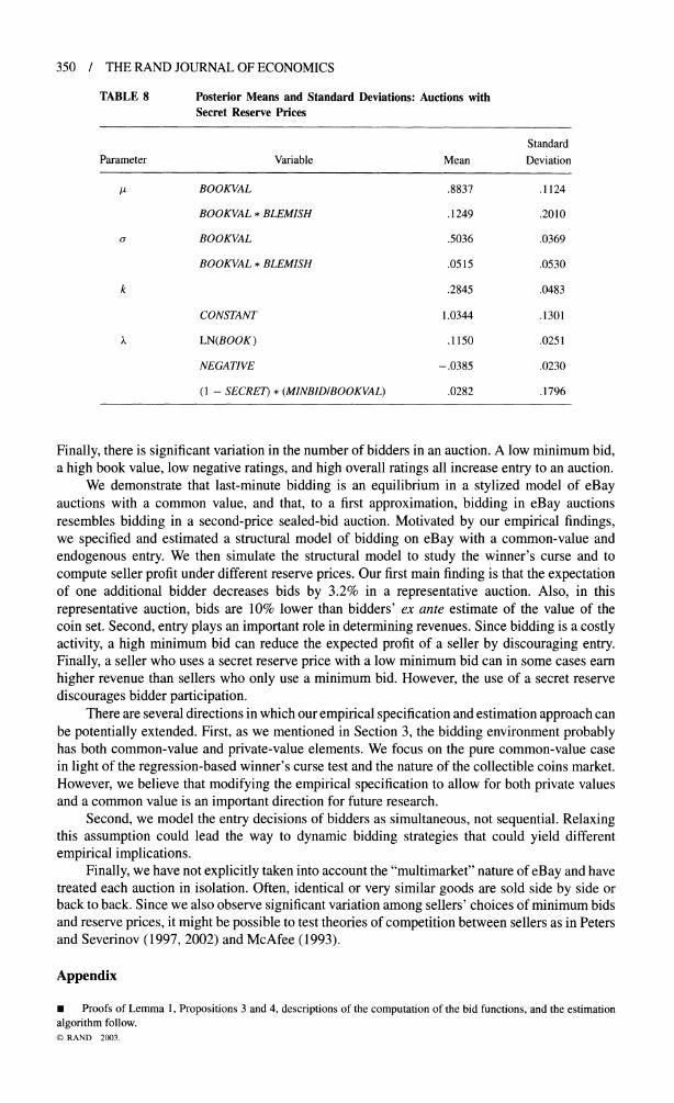
Our simulations of the effect of a secret reserve will be misleading if the secret reserve price is not exogenous. The results of Milgrom and Weber (1982) suggest that sellers should not intentionally hide information from bidders; otherwise, they will be punished with lower expected sale prices. However, since bidding on eBay is probably more complicated than the Milgrom and Weber model, it is not clear whether real-life sellers will follow this policy. In Table 8, we reestimated the structural model using only data from auctions with a secret reserve price.
The main difference we find is that the estimated mean valuation of the coins, as a percent of the book value of the item, is lower for items sold with a secret reserve (88% of book value), as opposed to the entire sample (99% of book value). Observe, however, that this estimation is done using many fewer data points, and the posterior standard deviation is 11%, bringing the posterior mean of the full sample estimates within a standard deviation. Regardless of the "significance" of the difference between parameter estimates, this result is consistent with the fact that sale prices of secret reserve items are lower (91% of book value) than items sold without a secret reserve (96% of book value). Coupled with the fact that 50% of secret reserve items go unsold, this could be a sign that sellers are willing to bear the cost of repeatedly relisting lower-quality but high- book-value items in order to "catch" a bidder with an unusually high valuation. Another plausible interpretation is that the change in the coefficients is due to fact that our parametric model is not completely flexible.36
7. Conclusion * In this article we study the determinants of bidder and seller behavior on eBay using a unique dataset of eBay coin auctions. Our research strategy has three parts. First, we describe a number of empirical regularities in bidder and seller behavior. Second, we develop a structural econometric model of bidding in eBay auctions. Third, we use this model to quantify the magnitude of the winner's curse and to simulate seller profit under different reserve prices.
There are a number of clear empirical patterns in our data. First, bidders engage in "sniping," submitting their bids close to the end of the auction. Second, there are some surprising patterns in how sellers set reserve prices. Sellers tend to set minimum bids at levels considerably less than the items' book values. Also, sellers tend to limit the use of secret reserve prices to high-value objects.
36 Our analysis abstracts away from the problem of whether the seller chooses to draw a signal xi about the object's worth. We assume that in the model of auctions with no secret reserve, the seller does not draw a signal xi, and in the model with a secret reserve, the seller does draw a signal. The seller's decision about whether or not to draw such a signal, and the bidder's beliefs about the seller's signal (or lack thereof), can lead to alternative specifications of the structural model. ? RAND 2003.
350 / THE RAND JOURNAL OF ECONOMICS
TABLE 8 Posterior Means and Standard Deviations: Auctions with Secret Reserve Prices
Standard Parameter Variable Mean Deviation
,I BOOKVAL .8837 .1124
BOOKVAL * BLEMISH .1249 .2010
a BOOKVAL .5036 .0369
BOOKVAL * BLEMISH .0515 .0530
k .2845 .0483
CONSTANT 1.0344 .1301
A LN(BOOK ) .1150 .0251
NEGATIVE -.0385 .0230
(1 - SECRET) * (MINBID/BOOKVAL) .0282 .1796
Finally, there is significant variation in the number of bidders in an auction. A low minimum bid, a high book value, low negative ratings, and high overall ratings all increase entry to an auction.
We demonstrate that last-minute bidding is an equilibrium in a stylized model of eBay auctions with a common value, and that, to a first approximation, bidding in eBay auctions resembles bidding in a second-price sealed-bid auction. Motivated by our empirical findings, we specified and estimated a structural model of bidding on eBay with a common-value and endogenous entry. We then simulate the structural model to study the winner's curse and to compute seller profit under different reserve prices. Our first main finding is that the expectation of one additional bidder decreases bids by 3.2% in a representative auction. Also, in this representative auction, bids are 10% lower than bidders' ex ante estimate of the value of the coin set. Second, entry plays an important role in determining revenues. Since bidding is a costly activity, a high minimum bid can reduce the expected profit of a seller by discouraging entry. Finally, a seller who uses a secret reserve price with a low minimum bid can in some cases earn higher revenue than sellers who only use a minimum bid. However, the use of a secret reserve discourages bidder participation.
There are several directions in which our empirical specification and estimation approach can be potentially extended. First, as we mentioned in Section 3, the bidding environment probably has both common-value and private-value elements. We focus on the pure common-value case in light of the regression-based winner's curse test and the nature of the collectible coins market. However, we believe that modifying the empirical specification to allow for both private values and a common value is an important direction for future research.
Second, we model the entry decisions of bidders as simultaneous, not sequential. Relaxing this assumption could lead the way to dynamic bidding strategies that could yield different empirical implications.
Finally, we have not explicitly taken into account the "multimarket" nature of eBay and have treated each auction in isolation. Often, identical or very similar goods are sold side by side or back to back. Since we also observe significant variation among sellers' choices of minimum bids and reserve prices, it might be possible to test theories of competition between sellers as in Peters and Severinov (1997, 2002) and McAfee (1993).
Appendix
* Proofs of Lemma 1, Propositions 3 and 4, descriptions of the computation of the bid functions, and the estimation algorithm follow. ? RAND 2003.
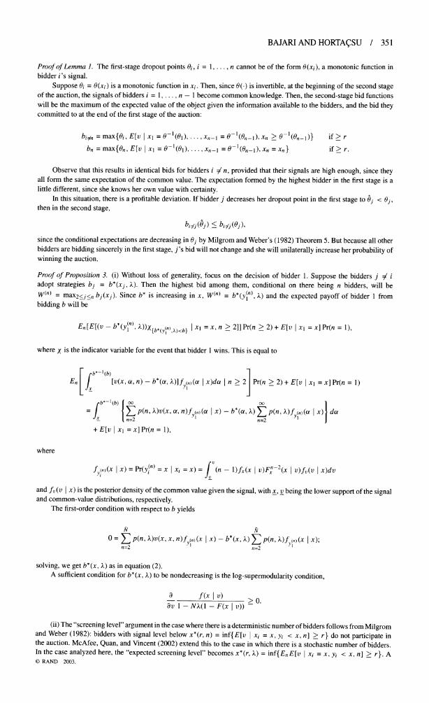
BAJARI AND HORTACSU / 351
Proof of Lemma 1. The first-stage dropout points Oi, i = 1, .., n cannot be of the form 0(xi), a monotonic function in bidder i's signal.
Suppose Oi = 0(xi) is a monotonic function in xi. Then, since 0(.) is invertible, at the beginning of the second stage of the auction, the signals of bidders i = 1,..., n - 1 become common knowledge. Then, the second-stage bid functions will be the maximum of the expected value of the object given the information available to the bidders, and the bid they committed to at the end of the first stage of the auction:
bin = max{0i, E[v I xl = 0-101) ..., Xn-_ =0-l(0n-1),Xn > 0-l(On-1)} if> r
bn = max{0n, E[v I xl = 0-1(01) ..., X_ = -l(0n-1), Xn = Xn} if > r.
Observe that this results in identical bids for bidders i / n, provided that their signals are high enough, since they all form the same expectation of the common value. The expectation formed by the highest bidder in the first stage is a little different, since she knows her own value with certainty.
In this situation, there is a profitable deviation. If bidder j decreases her dropout point in the first stage to 5j < Oj, then in the second stage,
bi~j(oj) < bij.6j(j),
since the conditional expectations are decreasing in Oj by Milgrom and Weber's (1982) Theorem 5. But because all other bidders are bidding sincerely in the first stage, j's bid will not change and she will unilaterally increase her probability of winning the auction.
Proof of Proposition 3. (i) Without loss of generality, focus on the decision of bidder 1. Suppose the bidders j =/ i adopt strategies bj = b*(xj, X). Then the highest bid among them, conditional on there being n bidders, will be Wn) = max2</<n bj(xj). Since b* is increasing in x, W) = b*(y(n), ) and the expected payoff of bidder 1 from bidding b will be
En[E[(v - b*(y), ))X{b(y(n))b} I l= x, n > 2]] Pr(n > 2) + E[v I x = x] Pr(n = 1),
where X is the indicator variable for the event that bidder 1 wins. This is equal to
b*-(b) En [v(x, , n)-b*(o, )]f(n)(O I x)dca n>2 Pr(n >2) + E[v x = x]Pr(n=1)
y I
,b*-1(b) 00 00
= I L p(n, X)v(x, a, n)fy(n)(a I x) - b*(a, A) p(n, A)f (n)((a Ix) do x- ,n=2 n=2
+ E[v xl =x]Pr(n= ),
where
fyn)(x | x)= Pr(y(n)= x Xi = x) (n - l) fx v)F x )f(v I x)dv
and fv(v I x) is the posterior density of the common value given the signal, with x, v being the lower support of the signal and common-value distributions, respectively.
The first-order condition with respect to b yields
N N O = , p(n, X)v(x, x, n)f(n)(X x)- b*(x, .) Ep(n, .)f (n)(x I X);
n=2 V n=2
solving, we get b*(x, X) as in equation (2). A sufficient condition for b*(x, .) to be nondecreasing is the log-supermodularity condition,
a f(xlv) > av 1 - N(1 - F(x I v)) -
(ii) The "screening level" argument in the case where there is a deterministic number of bidders follows from Milgrom and Weber (1982): bidders with signal level below x*(r, n) = inf{E[v I xi = x, Yi < x, n] > r} do not participate in the auction. McAfee, Quan, and Vincent (2002) extend this to the case in which there is a stochastic number of bidders. In the case analyzed here, the "expected screening level" becomes x*(r, X) = inf{EnE[v I xi = x, Yi < x, n] > r}. A ? RAND 2003.
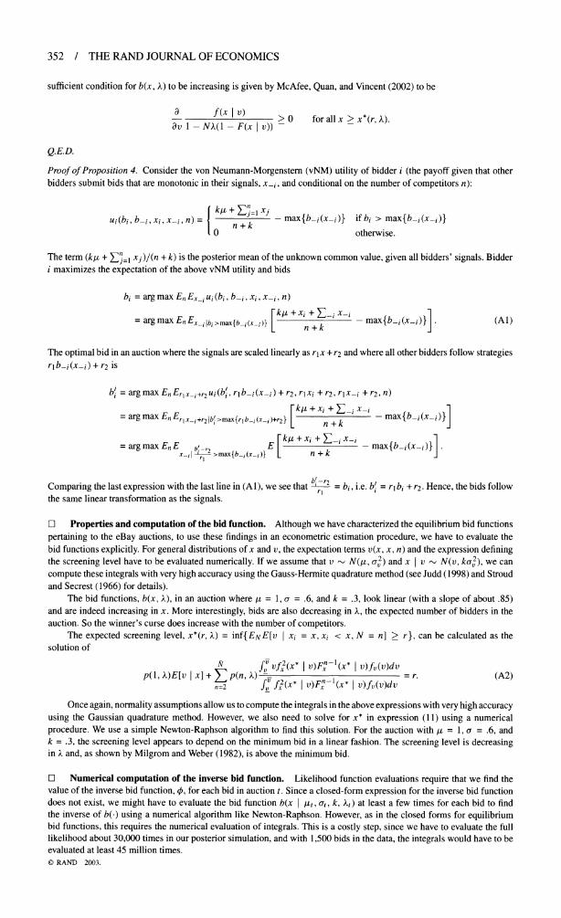
352 / THE RAND JOURNAL OF ECONOMICS
sufficient condition for b(x, A) to be increasing is given by McAfee, Quan, and Vincent (2002) to be
a - f -(x I v) ) > 0 for all x > x*(r, A). av 1 - NX(l - F(x I v)) -
Q.E.D.
Proof of Proposition 4. Consider the von Neumann-Morgenster (vNM) utility of bidder i (the payoff given that other bidders submit bids that are monotonic in their signals, x_i, and conditional on the number of competitors n):
kz + j= ix u(bi,b-i, i,x-i,n)= += - max{b_i(x_)} ifbi > max{b_i(x_i)}
0 otherwise.
The term (kA, + ,j=l xj)/(n + k) is the posterior mean of the unknown common value, given all bidders' signals. Bidder i maximizes the expectation of the above vNM utility and bids
bi = arg max En E_i ui(bi, b-i, xi, x-i, n)
= argmax En Exi bi ax{b( } i -max{b-i(x-)} (Al)
The optimal bid in an auction where the signals are scaled linearly as r1x + r2 and where all other bidders follow strategies rlb-i(x-i) + r2 is
bl = arg max EnErlx_i+r2ui(bl, rlb-i(x-i) + r2, rlxi + r2, rlx-i + r2, n)
= argmax EnEr-i_,+r2,b>max{rbi (xi )+r2} x+
-ixi max{b_i(x_i)}J n + k
= argmax EnE br E - max{b-i(x_-)} . x_i I l2
>max{b_i(x_i)} n + k
Comparing the last expression with the last line in (Al), we see that - r2 = bi, i.e. b' = rl bi + r2. Hence, the bids follow the same linear transformation as the signals.
O Properties and computation of the bid function. Although we have characterized the equilibrium bid functions
pertaining to the eBay auctions, to use these findings in an econometric estimation procedure, we have to evaluate the bid functions explicitly. For general distributions of x and v, the expectation terms v(x, x, n) and the expression defining the screening level have to be evaluated numerically. If we assume that v ~ N(,/, oa2) and x I v ~ N(v, ka2), we can
compute these integrals with very high accuracy using the Gauss-Hermite quadrature method (see Judd (1998) and Stroud and Secrest (1966) for details).
The bid functions, b(x, A), in an auction where ,i = 1, a = .6, and k = .3, look linear (with a slope of about .85) and are indeed increasing in x. More interestingly, bids are also decreasing in A, the expected number of bidders in the auction. So the winner's curse does increase with the number of competitors.
The expected screening level, x*(r, A) = inf{ENE[v xi = x, xi < x, N = n] > r}, can be calculated as the solution of
N fvf(x v)Fx 1(X* v)fv(v)dv2 p(l, )E[v x] + p(n, X) vf rf2(
x * (A2) n=2 fVU f \2(X. v)Fn-'(x* I v)fv(v)dv
Once again, normality assumptions allow us to compute the integrals in the above expressions with very high accuracy using the Gaussian quadrature method. However, we also need to solve for x* in expression (11) using a numerical procedure. We use a simple Newton-Raphson algorithm to find this solution. For the auction with it = 1, a = .6, and k = .3, the screening level appears to depend on the minimum bid in a linear fashion. The screening level is decreasing in X and, as shown by Milgrom and Weber (1982), is above the minimum bid.
O Numerical computation of the inverse bid function. Likelihood function evaluations require that we find the value of the inverse bid function, X, for each bid in auction t. Since a closed-form expression for the inverse bid function does not exist, we might have to evaluate the bid function b(x I tit, at, k, At) at least a few times for each bid to find the inverse of b(.) using a numerical algorithm like Newton-Raphson. However, as in the closed forms for equilibrium bid functions, this requires the numerical evaluation of integrals. This is a costly step, since we have to evaluate the full likelihood about 30,000 times in our posterior simulation, and with 1,500 bids in the data, the integrals would have to be evaluated at least 45 million times. ? RAND 2003.
BAJARI AND HORTACSU / 353
To reduce the computational complexity, we first exploit the linearity property of the bid functions. Recall that linearity implies that if b(x I Ai?, a?, k, A) is a pure-strategy equilibrium bid function to the auction where the common value is distributed normally with mean u?o and standard deviation a?, then rlb(rlx + r2 I ,?, o?, k, A) + r2 is the equilibrium bid function in the auction where the common value is distributed with mean rl L? + r2 and standard deviation r a?. This holds whether there is a known or random number of bidders in the auction. Similarly, if there is a posted reserve price in the auction, we can apply the linear transformation to the screening level x*(R, X, k). That is, if x*(R; ,z?, oa?, X, k) is the screening level in the original auction, then rlx*(rl R + r; I ,0, 0 k, )k + r2 will be the screening level in the transformed auction.
How does linearity help us? Suppose at a particular evaluation of the likelihood function, the distributional parameters are {[dt,rt} for auction t. Then we do not have to evaluate b(x I ,t, cr, k, X). Setting rl, = rt/a? and r2t = tLt, - rltP?, we interpolate the value of b((x - r2t)/rlt I I?, c?, k, X) from a set of precomputed values and return rltb((x-r2t)/rlt I ,?, cr0, k, A)+r2t. Assuming the interpolation is good enough, this scheme lets us avoid computing the Nash equilibrium in the course of likelihood function evaluations. The equilibrium is solved beforehand for a normalized set of parameter values and adapted to the parameter values generated by the posterior simulation routine.
When inverting the bid function, one can use a simple algorithm like Newton-Raphson with relative ease, since the bid function is monotonic and b(x) = x is usually a good starting value. Alternatively, one can evaluate b(x I ?o, a?, k, X) on the grid used for interpolation, and instead of using polynomial interpolation to find b as a function of x, k, X, one can use polynomial interpolation to evaluate x as a function of b, k, X. This allows one to approximate the inverse bid function directly, instead of having to evaluate the bid function several times until Newton-Raphson converges. This method is much more efficient in terms of calculating the derivative of the inverse bid function (the Jacobian), since the derivative of the polynomial interpolation can be written out in closed form and, once again, be evaluated in one step.
O Posterior simulation. Let
Xt = (SECRETt, BOOKVALt, BLEMISHt, NEGATIVEt, MINBIDt)
be the auction-specific data vector and let X denote the vector X = (X, ..., XT), where T is the total number of auctions. Let p(fB) denote the prior distribution of the parameters, L(BID I fB, X) denote the likelihood function, and p(P I BID, X) denote the posterior distribution of the vector of parameters fB conditional upon the observed data. By Bayes' theorem,
P(f I BID, X,) oc p(f)L(BID I 1, X).
That is, the posterior is proportional to the prior times the likelihood function. In many problems, we are interested in the expected value of some known function of the parameters which we represent as g(B):
E[g(p) I BIDSt, Xt] = f g(p)p(p I BID, X)df.
Examples include the posterior mean and standard deviation of fB or the expected revenue from an auction with a particular set of characteristics X. Recent work in Bayesian econometrics has developed methods to simulate the posterior distribution, so that integrals such as E[g(fB) I BIDSt, Xt] can be evaluated using Monte Carlo simulation. Posterior simulators generate a sequence of S pseudo-random vectors 1(1),.., . (S) from a Markov chain with the property that the invariant distribution of the chain is the posterior distribution p(p I BIDSt, Xt). Under regularity conditions discussed in Geweke (1997) (that are trivially satisfied in our application), it can be shown that
s= 15s) f lim s S = g(p)p(p I BID, X)dp. S- oo S
Therefore, the sample mean [ys=l g(lS)]/S is a consistent estimator of E[g(f) I BID, X].
O Priors. We assume that the prior is proportional to a constant if {0 < fB < 3}, {-2 < /2 < 2}, {0 < /3 < 2}, {-2 < 34 < 2}, {0 < P5 < 4}, and {0 < #6,7,8,9,10 < 5} and is equal to zero otherwise. We impose these flat priors to minimize the effect of prior choice on the shape of the posterior distribution. As for the appropriateness of the cutoff points, we made sure that these contained the "reasonable bounds" for the possible realizations of the parameters.
D Simulation. We used a variant of the Metropolis-Hastings algorithm to simulate the posterior distribution of the parameters. We start out by finding a rough approximation to the posterior mode, which we will refer to as /. The algorithm generates a sequence of S pseudo-random vectors PB(1), .(S) from a Markov chain. First set B() = , then generate the other simulations as follows:
(i) Given 4(n), draw a candidate value ff from a normal distribution with mean 1(n) and variance-covariance matrix -H-1.
? RAND 2003.
354 / THE RAND JOURNAL OF ECONOMICS
(ii) Let
a = m p(P( I BID, X)
o=mim| np(B(n) I BID, X)' i (iii) Set B(n+l) = fi with probability a.
(iv) Return to 1.
Geweke (1997) provides sufficient conditions for the invariant distribution of this chain to be the posterior distribution. It is easy to check that these conditions are satisfied in this application.
References
ATHEY, S. AND HAILE, P.A. "Identification of Standard Auction Models." Econometrica, Vol. 70 (2002), pp. 2107-2140. BAJARI, P. "The First Price Auction with Asymmetric Bidders: Theory and Applications." Ph.D. dissertation, University
of Minnesota, 1997. AND HORTACSU, A. "The Winner's Curse, Reserve Prices and Endogenous Entry: Empirical Insights From eBay
Auctions." Working Paper no. 00-004, Stanford University, 2000. BRYAN, D., LUCKING-REILEY, D., PRASAD, N., AND REEVES, D. "Pennies from eBay." Working Paper, Vanderbilt
University, 2000. DONALD, S.G. AND PAARSCH, H.J. "Piecewise Pseudo-maximum Likelihood Estimation in Empirical Models of Auctions."
International Economic Review, Vol. 34 (1993), pp. 121-148. ELYAKIME, B., LAFFONT, J.-J., LOISEL, P., AND VUONG, Q. "First-Price Sealed-Bid Auctions with Secret Reservation
Prices." Annales d'Economie et de Statistique, Vol. 34 (1994), pp. 115-141. GEWEKE, J. "Posterior Simulators in Econometrics." In D.M. Kreps and K.F. Wallis, eds., Advances in Economics and
Econometrics: Theory and Applications. Seventh World Congress. New York: Cambridge University Press, 1997. HAILE, P. AND TAMER, E. "Inference With an Incomplete Model of English Auctions." Journal of Political Economy, Vol.
111 (2003), pp. 1-51. , HONG, H., AND SHUM, M. "Nonparametric Tests for Common Values in First-Price Auctions." Mimeo, March
2000. HARSTAD, R.M. "Alternative Common-Value Auction Procedures: Revenue Comparisons with Free Entry." Journal of
Political Economy, Vol. 98 (1990), pp. 421-429. HONG, H. AND SHUM, M. "Increasing Competition and the Winner's Curse: Evidence from Procurement." Review of
Economic Studies, Vol. 69 (2002), pp. 871-898.
HOUSER, D. AND WOODERS, J. "Reputation in Auctions: Theory and Evidence from eBay." Working Paper, University of Arizona, 2000.
JUDD, K.L. Numerical Methods in Economics. Cambridge, Mass.: MIT Press, 1998. KATKAR R. AND LUCKING-REILEY, D. "Public versus Secret Reserve Prices in eBay Auctions: Results from a Pokemon
Field Experiment." Working Paper, Vanderbilt University, 2000. LEVIN, D. AND SMITH, J.L. "Equilibrium in Auctions with Entry." American Economic Review, Vol. 84 (1994), pp.
585-599. LI, H. AND TAN, G. "Hidden Reserve Prices with Risk Averse Bidders." Working paper, University of British Columbia,
May 2000. LUCKING-REILEY, D.L. "Auctions on the Internet: What's Being Auctioned, and How?" Journal of Industrial Economics,
Vol. 48 (2000), pp. 227-252. MCAFEE, R.P. "Mechanism Design by Competing Sellers." Econometrica, Vol. 61 (1993), pp. 1281-1312. MELNICK, M.I. AND ALM, J."Does a Seller's eCommerce Reputation Matter? Evidence from eBay Auctions." Journal of
Industrical Economics, Vol. 50 (2002), pp. 337-350. ,QUAN, D., AND VINCENT, D. "How to Set Minimum Acceptable Bids with An Application to Real Estate
Auctions." Journal of Industrial Economics, forthcoming. MILGROM, P.R. AND WEBER, R.J. "A Theory of Auctions and Competitive Bidding." Econometrica, Vol. 50 (1982), pp.
1089-1122. MYERSON, R.B. "Optimal Auction Design." Mathematics of Operation Research, Vol. 6 (1981), pp. 58-73. PAARSCH, H.J. "Deciding Between the Common Value and Private Value Paradigms in Empirical Models of Auctions."
Journal of Econometrics, Vol. 51 (1992), pp. 191-215. PETERS, M. AND SEVERINOV, S. "Competition among Sellers Who Offer Auctions Instead of Prices." Journal of Economic
Theory, Vol. 75 (1997), pp. 141-179. AND . "Internet Auctions with Many Traders." Working Paper, University of Toronto, 2002.
PINSKE, J. AND TAN, G. "Fewer Bidders Can Increase Price in First-Price Auctions with Affiliated Private Values." Mimeo, 2000.
PORTER, J. AND HIRANO, K. "Asymptotic Efficiency in Parametric Structural Models With Parameter-Dependent Support." Working paper, Harvard University and UCLA, 2001.
RESNICK, P. AND ZECKHAUSER, R. "Trust Among Strangers in Internet Transactions: Empirical Analysis of eBay's Reputation System." Working Paper, University of Michigan, 2001.
? RAND 2003.
BAJARI AND HORTA(SU / 355
, SWANSON, J., AND LOCKWOOD, K. "The Value of Reputation on eBay: A Controlled Experiment." Working Paper, University of Michigan, 2002.
ROTH, A. AND OCKENFELS, A. "Last Minute Bidding and the Rules for Ending Second-Price Auctions: Theory and Evidence from a Natural Experiment on the Internet." NBER Working Paper no. W7729, 2000.
STROUD, A.H. AND SECREST, D. Gaussian Quadrature Formulas. Englewood Cliffs, N.J.: Prentice-Hall, 1966.
VINCENT, D.R. "Bidding Off the Wall: Why Reserve Prices May Be Kept Secret." Journal of Economic Theory, Vol. 65
(1995), pp. 575-584. WILSON, R. "A Bidding Model of Perfect Competition." Review of Economic Studies, Vol. 44 (1977), pp. 511-518.
WOLVERTON, T. "eBay Users Miffed by New Fees." CNET News.com, August 20, 1999 (http://news.com.com/ 2100- 1017-230100.htm).
? RAND 2003.