of housing supply - center for real estate housing supply ∗ albert saiz i ... a housing supply...

THE GEOGRAPHIC DETERMINANTSOF HOUSING SUPPLY∗

ALBERT SAIZ

I process satellite-generated data on terrain elevation and presence of waterbodies to precisely estimate the amount of developable land in U.S. metropolitanareas. The data show that residential development is effectively curtailed by thepresence of steep-sloped terrain. I also find that most areas in which housingsupply is regarded as inelastic are severely land-constrained by their geography.Econometrically, supply elasticities can be well characterized as functions of bothphysical and regulatory constraints, which in turn are endogenous to prices anddemographic growth. Geography is a key factor in the contemporaneous urbandevelopment of the United States.

I. INTRODUCTION

The determinants of local housing supply elasticities are ofcritical importance in explaining current trends in the shape ofurban development and the evolution of housing values.1 Theexisting literature on this topic has focused on the role that lo-cal land use regulations play in accounting for differences in theavailability of land. The large variance in housing values acrosslocales can indeed be partially explained by man-made regula-tory constraints. However, zoning and other land-use policies aremultidimensional, difficult to measure, and endogenous to preex-isting land values. In this context, it is uncontroversial to arguethat predetermined geographic features such as oceans, lakes,mountains, and wetlands can also induce a relative scarcity of de-velopable land. Hence their study merits serious consideration: towhat extent, if at all, does geography determine contemporaneouspatterns of urban growth?2

This paper gives empirical content to the concepts of landscarcity and abundance in urban America. Using geographic infor-mation system (GIS) techniques, I precisely estimate the area thatis forgone to the sea within 50-kilometer radii from metropolitan

∗Enestor Dos Santos and Blake Willmarth provided superb research assis-tance. The editor, three referees, Matt White, Joe Gyourko, Jeff Zabel, and partic-ipants at the 2008 ASSA, EEA, and NBER meetings provided helpful input. Allerrors are my sole responsibility. I gratefully acknowledge financial help from theZell–Lurie Center Research Sponsors Fund.

1. Glaeser, Gyourko, and Saks (2006); Saks (2008).2. An important step in this direction has been taken by Burchfield et al.

(2006), who relate terrain ruggednes and access to underground water to thedensity and compactness of new real estate development.

C© 2010 by the President and Fellows of Harvard College and the Massachusetts Institute ofTechnology.The Quarterly Journal of Economics, August 2010

1253

at MIT

Libraries on January 8, 2014

http://qje.oxfordjournals.org/D

ownloaded from

http://qje.oxfordjournals.org/


1254 QUARTERLY JOURNAL OF ECONOMICS

central cities. I then use satellite-based geographic data on landuse provided by the United States Geographic Service (USGS)to calculate the area lost to internal water bodies and wetlands.Using the USGS Digital Elevation Model (DEM) at 90–squaremeter cell grids, I also create slope maps, which allow me to calcu-late how much of the land around each city exhibits slopes above15%. Combining all the information above, the paper providesa precise measure of exogenously undevelopable land in cities.I then turn to studying the links between geography and urbandevelopment.

To do so, I first develop a conceptual framework that relatesland availability to urban growth and housing prices. Using avariation of the Alonso–Muth–Mills model (Alonso 1964; Mills1967; Muth 1969), I show that land-constrained cities not onlyshould be more expensive ceteris paribus, but also should dis-play lower housing supply elasticities with respect to citywidedemand shocks, a somewhat ad hoc claim in the existing litera-ture. I also show that, in equilibrium, consumers in geographicallyconstrained metropolitan areas should require higher wages orhigher amenities to compensate them for more expensive housing.

Empirically, all of these facts are corroborated by the data. Ifind that most areas that are widely regarded as supply-inelasticare, in fact, severely land-constrained by their geography. Rose(1989b) showed a positive correlation between coastal constraintsand housing prices for a limited sample of forty-five cities. Here Ishow that restrictive geography, including the presence of moun-tainous areas and internal water, was a very strong predictor ofhousing price levels and growth for all metropolitan statistical ar-eas (MSA) during the period 1970–2000, even after controlling forregional effects. This association was not solely driven by coastalareas, as it is present even within coastal markets. I next deploythe Wharton Residential Urban Land Regulation Index recentlycreated by Gyourko, Saiz, and Summers (2008). The index is con-structed to capture the stringency of residential growth controls.Using alternate citywide demand shocks, I estimate metropolitan-specific housing supply functions and find that housing supplyelasticities can be well characterized as functions of both physicaland regulatory constraints.

These associations, however, do not take into account feed-back effects between prices and regulations. Homeowners havestronger incentives to protect their housing investments whereland values are high initially. The homevoter hypothesis (Fischel

at MIT



ownloaded from



THE GEOGRAPHIC DETERMINANTS OF HOUSING SUPPLY 1255

2001) implies a reverse causal relationship from initially highland values to increased regulations. Empirically, I find thatantigrowth local land policies are more likely to arise in growing,land-constrained metropolitan areas and in cities where preex-isting land values were high and worth protecting. Hence, I nextendogeneize the regulatory component of housing supply elastic-ity. I posit and estimate an empirical model of metropolitan hous-ing markets with endogenous regulations. As exogenous land-useregulatory shifters, I use measures shown to be associated withlocal tastes for regulation. Both geography and regulation are im-portant to account for housing supply elasticities, with the lattershowing themselves to be endogenous to prices and past growth.

Finally, I use the results to provide operational estimates oflocal supply elasticities in all major U.S. metropolitan areas. Theseestimates, based on land-availability fundamentals, should proveuseful in calibrating general equilibrium models of interregionallabor mobility and in predicting the response of housing mar-kets to future demand shocks. Housing supply is estimated to bequite elastic for the average metropolitan area (with a population-weighted elasticity of 1.75). In land-constrained large cities, suchas cities in coastal California, Miami, New York, Boston, andChicago, estimated elasticities are below one. These elasticityestimates display a very strong correlation of .65 with housingprices in 2000. Quantitatively, a movement across the interquar-tile range in geographic land availability in an average-regulatedmetropolitan area of 1 million is associated with shifting froma housing supply elasticity of approximately 2.45 to one of 1.25.Moving to the ninetieth percentile of land constraints (as in SanDiego, where 60% of the area within its 50-km radius is not devel-opable) pushes average housing supply elasticities down furtherto 0.91. The results in the paper ultimately demonstrate that geog-raphy is a key factor in the contemporaneous urban developmentof the United States.

II. GEOGRAPHY AND LAND IN THE UNITED STATES: A NEW DATA SET

The economic importance of geography for local economic de-velopment is an underexplored topic. Previous research has ex-amined the correlation between housing price levels and proxiesfor the arc of circle lost to the sea in a limited number of cities(Rose 1989a, 1989b; Malpezzi 1996; Malpezzi, Chun, and Green1998) but the measures proved somewhat limited. Recent papers

at MIT



ownloaded from




in urban economics, such as Burchfield et al. (2006), Rosenthal andStrange (2008), and Combes et al. (2009), underline the relevanceof geographic conditions as economic fundamentals explaining lo-cal population density.

Here, I develop a comprehensive measure of the area that isunavailable for residential or commercial real estate developmentin MSAs. Architectural development guidelines typically deem ar-eas with slopes above 15% severely constrained for residentialconstruction. Using data on elevation from the USGS Digital Ele-vation Model (DEM) at its 90-m resolution, I generated slope mapsfor the continental United States. GIS software was then used tocalculate the exact share of the area corresponding to land withslope above 15% within a 50-km radius of each metropolitan cen-tral city.

Residential development is effectively constrained by thepresence of steep slopes. To demonstrate this, I focus on Los An-geles (LA). Median housing values there are among the highest inthe United States and the incentives to build on undeveloped landare very strong. Using GIS software to delineate the intersectionbetween steep-slope zones and the 6,456 census block groups (asdelimited in 2000) that lie within a 50-km radius of LA’s city cen-troid, I calculated the share of the area in each block group withslope above 15%. Then I defined steep-slope block groups as thosewith a share of steep-sloped terrain of more than 50%. Steep-slopeblock groups encompassed 47.62% of the land area within 50 km ofLA’s geographic center in year 2000. However, only 3.65% of thepopulation within this 50-km radius lived in them. These mag-nitudes clearly illustrate the deterrent effect of steep slopes onhousing development.

The next step to calculate land availability involved esti-mating the area within the cities’ 50-km radii that correspondsto wetlands, lakes, rivers, and other internal water bodies. The1992 USGS National Land Cover Dataset is a satellite-based GISsource containing information about land cover characteristicsat 30 by 30–m cell resolutions. The data were processed by theWharton GIS lab to produce information on the area apportionedto each of the land cover uses delimited by the USGS by censustract. Next, the distance from each central city centroid to the cen-troid of all census tracts was calculated, and Census tracts within50 km were used to compute water cover shares.

Last, I used digital contour maps to calculate the areas withinthe 50-km radii that are lost to oceans and the Great Lakes. The

at MIT



ownloaded from




final measure combines the area corresponding to steep slopes,oceans, lakes, wetlands, and other water features. This is the firstcomprehensive measure of truly undevelopable area in the litera-ture. The use of a radius from the city centroid makes it a measureof original constraints, as opposed to one based on ex post ease ofdevelopment (e.g., density).

Table I displays the percentages of undevelopable area for allMSAs with population over 500,000 in the 2000 Census for which Ialso have regulation data (those included in the later regressions).Of these large metro areas, Ventura (CA) is the most constrained,with 80% of the area within a 50-km radius rendered undevel-opable by the Pacific Ocean and mountains. Miami, Fort Laud-erdale, New Orleans, San Francisco, Sarasota, Salt Lake City,West Palm Beach, San Diego, and San Jose complete the list ofthe top 10 most physically constrained major metropolitan areasin the United States. Many large cities in the South and Mid-west (such as Atlanta, San Antonio, and Columbus) are largelyunconstrained.

Table II studies the correlates of the newly constructed landunavailability variable. To do so, I run a number of indepen-dent regressions. The variables in Table II’s rows appear on theleft-hand side in each sequential regression, and the geographic-unavailability variable is always the main right-hand side con-trol. Regional fixed effects (Northeast, South, Midwest, West) areincluded in all regressions. Each column shows the coefficientof the variable of reference on the unavailable land share, andits associated standard error appears in parentheses. A secondset of regressions (2) also controls for a coastal status dummy,which identifies metropolitan areas that are within 100 km of theocean or Great Lakes. The significant coefficients reveal that geo-graphically land-constrained areas tended to be more expensive in2000, to have experienced faster price growth since 1970, to havehigher incomes, to be more creative (higher patents per capita),and to have higher leisure amenities (as measured by the numberof tourist visits).3 Observed metropolitan population levels werelargely orthogonal to natural land constraints.

Interestingly, note that none of the major demand-side driversof recent urban demographic change (immigration, education,

3. Carlino and Saiz (2008) demonstrate that the number of tourist visits isstrongly correlated with other measures of quality of life and a strong predictor ofrecent city growth.

at MIT



ownloaded from




TA

BL

EI

PH

YS

ICA

LA

ND

RE

GU

LA

TO

RY

DE

VE

LO

PM

EN

TC

ON

ST

RA

INT

S(M

ET

RO

AR

EA

SW

ITH

PO

PU

LA

TIO

N>

500,

000)

Un

deve

lopa

ble

Un

deve

lopa

ble

Ran

kM

SA

/NE

CM

An

ame

area

(%)

WR

IR

ank

MS

A/N

EC

MA

nam

ear

ea(%

)W

RI

1V

entu

ra,C

A79

.64

1.21

26P

ortl

and–

Van

cou

ver,

OR

–WA

37.5

40.

272

Mia

mi,

FL

76.6

30.

9427

Tac

oma,

WA

36.6

91.

343

For

tL

aude

rdal

e,F

L75

.71

0.72

28O

rlan

do,F

L36

.13

0.32

4N

ewO

rlea

ns,

LA

74.8

9−1

.24

29B

osto

n–W

orce

ster

–Law

ren

ce,M

A–N

H33

.90

1.70

5S

anF

ran

cisc

o,C

A73

.14

0.72

30Je

rsey

Cit

y,N

J33

.80

0.29

6S

alt

Lak

eC

ity–

Ogd

en,U

T71

.99

−0.0

331

Bat

onR

ouge

,LA

33.5

2−0

.81

7S

aras

ota–

Bra

den

ton

,FL

66.6

30.

9232

Las

Veg

as,N

V–A

Z32

.07

−0.6

98

Wes

tP

alm

Bea

ch–B

oca

Rat

on,F

L64

.01

0.31

33G

ary,

IN31

.53

−0.6

99

San

Jose

,CA

63.8

00.

2134

New

ark,

NJ

30.5

00.

6810

San

Die

go,C

A63

.41

0.46

35R

och

este

r,N

Y30

.46

−0.0

611

Oak

lan

d,C

A61

.67

0.62

36P

itts

burg

h,P

A30

.02

0.10

12C

har

lest

on–N

orth

Ch

arle

ston

,SC

60.4

5−0

.81

37M

obil

e,A

L29

.32

−1.0

013

Nor

folk

–Vir

gin

iaB

each

–New

port

59.7

70.

1238

Scr

anto

n–W

ilke

s-B

arre

–Haz

leto

n,P

A28

.78

0.01

New

s,V

A–N

C14

Los

An

gele

s–L

ong

Bea

ch,C

A52

.47

0.49

39S

prin

gfiel

d,M

A27

.08

0.72

15V

alle

jo–F

airfi

eld–

Nap

a,C

A49

.16

0.96

40D

etro

it,M

I24

.52

0.05

16Ja

ckso

nvi

lle,

FL

47.3

3−0

.02

41B

aker

sfiel

d,C

A24

.21

0.40

17N

ewH

aven

–Bri

dgep

ort–

Sta

mfo

rd,C

T45

.01

0.19

42H

arri

sbu

rg–L

eban

on–C

arli

sle,

PA

24.0

20.

5418

Sea

ttle

–Bel

levu

e–E

vere

tt,W

A43

.63

0.92

43A

lban

y–S

chen

ecta

dy–T

roy,

NY

23.3

3−0

.09

19M

ilw

auke

e–W

auke

sha,

WI

41.7

80.

4644

Har

tfor

d,C

T23

.29

0.49

20T

ampa

–St.

Pet

ersb

urg

–Cle

arw

ater

,FL

41.6

4−0

.22

45T

ucs

on,A

Z23

.07

1.52

21C

leve

lan

d–L

orai

n–E

lyri

a,O

H40

.50

−0.1

646

Col

orad

oS

prin

gs,C

O22

.27

0.87

22N

ewY

ork,

NY

40.4

20.

6547

Bal

tim

ore,

MD

21.8

71.

6023

Ch

icag

o,IL

40.0

10.

0248

All

ento

wn

–Bet

hle

hem

–Eas

ton

,PA

20.8

60.

0224

Kn

oxvi

lle,

TN

38.5

3−0

.37

49M

inn

eapo

lis–

St.

Pau

l,M

N–W

I19

.23

0.38

25R

iver

side

–San

Ber

nar

din

o,C

A37

.90

0.53

50B

uff

alo–

Nia

gara

Fal

ls,N

Y19

.05

−0.2

3

at MIT



ownloaded from



THE GEOGRAPHIC DETERMINANTS OF HOUSING SUPPLY 1259T

AB

LE

I(C

ON

TIN

UE

D)

Un

deve

lopa

ble

Un

deve

lopa

ble

Ran

kM

SA

/NE

CM

An

ame

area

(%)

WR

IR

ank

MS

A/N

EC

MA

nam

ear

ea(%

)W

RI

51T

oled

o,O

H18

.96

−0.5

774

Dal

las,

TX

9.16

−0.2

352

Syr

acu

se,N

Y17

.85

−0.5

975

Ric

hm

ond–

Pet

ersb

urg

,VA

8.81

−0.3

853

Den

ver,

CO

16.7

20.

8476

Hou

ston

,TX

8.40

−0.4

054

Col

um

bia,

SC

15.2

3−0

.76

77R

alei

gh–D

urh

am–C

hap

elH

ill,

NC

8.11

0.64

55W

ilm

ingt

on–N

ewar

k,D

E–M

D14

.67

0.47

78A

kron

,OH

6.45

0.07

56B

irm

ingh

am,A

L14

.35

−0.2

379

Tu

lsa,

OK

6.29

−0.7

857

Ph

oen

ix–M

esa,

AZ

13.9

50.

6180

Kan

sas

Cit

y,M

O–K

S5.

82−0

.79

58W

ash

ingt

on,D

C–M

D–V

A–W

V13

.95

0.31

81E

lPas

o,T

X5.

130.

7359

Pro

vide

nce

–War

wic

k–P

awtu

cket

,RI

13.8

71.

8982

For

tW

orth

–Arl

ingt

on,T

X4.

91−0

.27

60L

ittl

eR

ock–

Nor

thL

ittl

eR

ock,

AR

13.7

1−0

.85

83C

har

lott

e–G

asto

nia

–Roc

kH

ill,

4.69

−0.5

3N

C–S

C61

Fre

sno,

CA

12.8

80.

9184

Atl

anta

,GA

4.08

0.03

62G

reen

vill

e–S

part

anbu

rg–

12.8

7−0

.94

85A

ust

in–S

anM

arco

s,T

X3.

76−0

.28

An

ders

on,S

C63

Nas

hvi

lle,

TN

12.8

3−0

.41

86O

mah

a,N

E–I

A3.

34−0

.56

64L

ouis

vill

e,K

Y–IN

12.6

9−0

.47

87S

anA

nto

nio

,TX

3.17

−0.2

165

Mem

phis

,TN

–AR

–MS

12.1

81.

1888

Gre

ensb

oro–

Win

ston

–Sal

em–

3.12

−0.2

9H

igh

Poi

nt,

NC

66S

tock

ton

–Lod

i,C

A12

.05

0.59

89F

ort

Way

ne,

IN2.

56−1

.22

67A

lbu

quer

que,

NM

11.6

30.

3790

Col

um

bus,

OH

2.50

0.26

68S

t.L

ouis

,MO

–IL

11.0

8−0

.73

91O

klah

oma

Cit

y,O

K2.

46−0

.37

69Y

oun

gsto

wn

–War

ren

,OH

10.5

2−0

.38

92W

ich

ita,

KS

1.66

−1.1

970

Cin

cin

nat

i,O

H–K

Y–IN

10.3

0−0

.58

93In

dian

apol

is,I

N1.

44−0

.74

71P

hil

adel

phia

,PA

–NJ

10.1

61.

1394

Day

ton

–Spr

ingfi

eld,

OH

1.04

−0.5

072

An

nA

rbor

,MI

9.71

0.31

95M

cAll

en–E

din

burg

–Mis

sion

,TX

0.93

−0.4

573

Gra

nd

Rap

ids–

Mu

skeg

on–H

olla

nd,

MI

9.28

−0.1

5

Not

e.W

RI

=W

har

ton

Reg

ula

tion

Inde

x.

at MIT



ownloaded from




TABLE IIPARTIAL CORRELATES OF UNAVAILABLE LAND SHARE (50-KM RADIUS)

Share of area unavailable for development

OLS-regional FE Adds coastal dummyβ β

(1) (2)

Log population in 2000 0.443 −0.01(0.336) (0.364)

Log median house value in 2000 0.592 0.41(0.081)∗∗∗ (0.085)∗∗∗

�Log median house value 0.240 0.122(1970–2000) (0.054)∗∗∗ (0.057)∗∗

Log income in 2000 0.233 0.164(0.056)∗∗∗ (0.060)∗∗∗

�Log income (1990–2000) −0.002 0.006(0.020) (0.022)

�Log population (1990–2000) −0.027 −0.043(0.027) (0.029)

Immigrants (1990–2000)/population 0.009 −0.007(1990) (0.011) (0.012)

Share with bachelor’s degree (2000) 0.006 −0.004(0.020) (0.022)

Share workers in manufacturing −0.01 0.005(2000) (0.021) (0.023)

Log(patents/population) (2000) 0.762 0.771(0.260)∗∗∗ (0.287)∗∗∗

January monthly hours of sun −3.812 −12.047(average 1941–1970) (11.252) (12.318)

Log tourist visits per person (2000) 0.493 0.719(0.261)∗ (0.286)∗∗

Notes. Standard errors in parentheses. Rows present the coefficients (β) and standard errors of separateregressions, where the variable described in the row is the dependent variable on the left-hand side andthe unavailable land share (geographic constraint) is the explanatory variable on the right-hand side. Theregressions in column (1) include regional fixed effects as controls, whereas those in column (2) also include acoastal dummy for metropolitan areas within 100 km of the oceans or Great Lakes (as defined in Rappaportand Sachs [2003]). ∗ significant at 10%; ∗∗ significant at 5%; ∗∗∗ significant at 1%.

manufacturing orientation, and hours of sun) was actually cor-related with geographic land constraints.

All results hold after controlling for the coastal dummy, indi-cating that the new land-availability variable contains informa-tion above and beyond that used in studies that focus on coastalstatus (Rose 1989a, 1989b; Malpezzi 1996). Taking into accountthe standard deviations of the different components of land un-availability, mountains contribute 42% of the variation in thisvariable, whereas coastal and internal water loss account for

at MIT



ownloaded from




31% and 26% of the variance in land constraints, respectively.After controlling for region fixed effects, as I do throughout thepaper, there is no correlation in the data between coastal arealoss and the extent of land constraints begotten by mountainousterrain. The loss of developable land due to the presence of largebodies of internal water (70% of which is attributable to wetlands,as in the Everglades) tends to be positively associated with coastalarea loss and, not surprisingly, negatively associated with moun-tainous terrain.

The other major data set used in the paper is obtained fromthe 2005 Wharton Regulation Survey. Gyourko, Saiz, and Sum-mers (2008) use the survey to produce a number of indexes thatcapture the intensity of local growth control policies in a numberof dimensions. Lower values in the Wharton Regulation Index,which is standardized across all municipalities in the originalsample, can be thought of as signifying the adoption of morelaissez-faire policies toward real estate development. Metropoli-tan areas with high values of the Wharton Regulation Index(WRI henceforth), conversely have zoning regulations or projectapproval practices that constrain new residential real estate de-velopment. I process the original municipal-based data to createaverage regulation indexes by metropolitan area using the proba-bility sample weights developed by Gyourko, Saiz, and Summers(2008).4

Table I displays the average WRI values for all metropolitanareas with populations greater than 500,000 and for which dataare available. A clear pattern arises when the regulation indexis contrasted with the land-availability measure. Physical landscarcity is associated with stricter regulatory constraints to de-velopment. Of the twenty most land-constrained areas, fourteenhave positive values of the regulation index (which has a mean of−0.10 and a s.e. of 0.81 across metro areas). Conversely, sixteen ofthe twenty least land-constrained metropolitan areas have nega-tive regulation index values.

Other data sources are used throughout the paper: the readeris referred to Appendices I–III for descriptive statistics and themeaning and provenance of the remaining variables.

4. Note that, because of different sample sizes across cities, in regressionswhere the WRI is used on the left-hand side (Table IV), heteroscedasticity could bean issue, and therefore Feasible Generalized Least Squares (FGLS) are used. Infact, however, the results in Table IV are very robust to all reasonable weightingschemes and the omission of metro areas with smaller number of observations inthe WRI.

at MIT



ownloaded from




III. GEOGRAPHY AND LOCAL DEVELOPMENT: A FRAMEWORK

Why should physical or man-made land availability con-straints have an impact on housing supply elasticities? How doesgeography shape urban development? To characterize the supplyof housing in a city, I assume developers to be price takers inthe land market. Consumers within the city compete for locationsdetermining the price of the land input. Taking land values andconstruction outlays as given, developers supply housing at cost.All necesary model derivations and the proofs of propositions arein the mathematical appendix, Appendix I.

The preferences of homogeneous consumers in city k are cap-tured by the utility function U (Ck) = (Ck)ρ . Consumption in thecity (Ck) is the sum of the consumption of city amenities (Ak) andprivate goods. Private consumption is equal to wages in the cityminus rents, minus the (monetized) costs of commuting to thecentral business district (CBD), where all jobs are located. Eachindividual is also a worker and lives in a separate house, so thatthe number of housing units equals population (Hk = POPk). Util-ity can be expressed as U (Ck) = (Ak + wk − γ · r′ − t · d)ρ , wherewk stands for the wage in the city, γ for the units of land/housing-space consumption (assumed constant), r′ for the rent per unitof housing-space consumption, t for the monetary cost per dis-tance commuted, and d for the distance of the consumer’s resi-dence to the CBD. As in conventional Alonso–Muth–Mills models(Brueckner 1987), a nonarbitrage condition defines the rent gra-dient: all city inhabitants attain utility Uk via competition inthe land markets. Therefore the total rent paid by an individual(r = γ · r′) takes the functional form r(d) = r0 − td.

Consider a circular city with radius �k. Geographic or reg-ulatory land constraints make construction unfeasible in someareas: only a sector (share) �k of the circle is developable.5 Thecity radius is thus a function of the number of households andland availability: �k = √

γ Hk/�kπ .Developers are price takers and buy land at market prices.

They build and sell homes at price P(d). The construction sectoris competitive and houses are sold at the cost of land, LC(d), plusconstruction costs, CC, which include the profits of the builder:P(d) = CC + LC(d). In the asset market steady state equilibrium

5. This feature appears in conventional urban economic models that focus ona representative city (Capozza and Helsley 1990). Here, I add heterogeneity inthe land availability parameter across cities and derive explicit housing supplieselasticities from it.

at MIT



ownloaded from




there is no uncertainty and prices equal the discounted value ofrents: P(d) = r(d)/i, which implies that r(d) = i · CC + i · LC(d).At the city’s edge there is no alternative use for land so, withoutloss of generality, LC(�k) = 0. Therefore r(�k) = i · CC, which im-plies that r0 = i · CC + t · √

γ Hk/�kπ .In this setup, average housing rent in the city, rk, can be shown

to be equivalent to the rent paid by the household living two-thirdsof the distance from the CBD to the city’s edge: rk = r( 2

3�k) (seeDerivation 1 in Appendix II). The final housing supply equation inthe city has average housing values (PS

k ) expressed as a functionof the number of households:

(1) PSk = CC + 1

3it ·

√γ Hk

�kπ.

I next define the aggregate demand function for housing inthe city. In a system of open cities, consumers can move and thusequalize utility across locations, which I normalize to zero (i.e.,the spatial indifference condition is Uk = 0 ∀k). Furthermore, inall cities, wk and Ak are functions of population. I model the levelof amenities as Ak = Ak − α

√POPk. The parameter α mediates the

marginal congestion cost (in terms of rivalry for amenities, traffic,pollution, noise, social capital dilution, crime, etc.). α could also beinterpreted in the context of an alternative but isomorphic modelwith taste heterogeneity: people with greater preferences for thecity are willing to pay more and move in first, but later marginalmigrants display less of a willingness to pay for the city (e.g.,Saiz [2007]). Labor demand is modeled as wk = wk − ψ

√POPk

and is assumed to be downward sloping; marginal congestioncosts weakly increase with population (ψ, α ≥ 0).6 Recalling thatHk = POPk, substituting into the intercity spatial equilibriumequation, and focusing w.o.l.o.g. on the spatial indifference condi-tion of consumers living in the CBD, I obtain the demand schedulefor housing in the city:

(2)√

Hk = Ak + wk

(ψ + α)− i

(ψ + α)P(0).

6. Of course, cities may display agglomeration economies up to some conges-tion point (given predetermined conditions, these may be captured by Ak + wk). Itis necessary only that, in equilibrium, the marginal effect of population on wagesand amenities be (weakly) negative. This is a natural assumption that avoids acounterfactual equilibrium where all activity is concentrated in one single citywith �k = 1.

at MIT



ownloaded from




Note that relative shocks to labor productivity or to amenities(Ak + wk) shift the city’s demand curve upward, which I will useto identify supply elasticities later.

I can now combine the expression for home values in the CBDvia the supply equation and the city-demand equation (2) to obtainthe equilibrium number of households in each city,

H∗k =

⎛⎝ Ak + wk − i · CC

(ψ + α) + t ·√

γ

�k·π

⎞⎠2

(Derivation 2).

Note that amenities and wages have to at least cover the an-nuitized physical costs of construction for a potential site to beinhabitable.

Within this setup, I first study the supply response to growthin the demand for housing that is induced by productivity andamenity shocks. Its is clear that ∂ P

Sk /∂�k < 0. Other things equal,

more land availability shifts down the supply schedule. Do landconstraints also have an effect with respect to supply elastici-ties? Defining the city-specific supply inverse elasticity of averagehousing prices as βS

k ≡ ∂ ln PSk /∂ ln Hk one can demonstrate

PROPOSITION 1. The inverse elasticity of supply (that is, the pricesensitivity to demand shocks) is decreasing in land availabil-ity. Conversely, as land constraints increase, positive demandshocks imply stronger positive impacts on the the growth ofhousing values.

Proposition 1 tells us that land-constrained cities have moreinelastic housing supply and helps us understand how housingprices react to exogenous demand shocks. In addition, two inter-esting further questions arise from the general equilibrium inthe housing and labor markets: Why is there any population inareas with difficult housing supply conditions? Should these ar-eas be more expensive ex post in equilibrium? Assume that thecovariance between productivity, amenities, and land availabil-ity is zero across all locales. Productivity–amenity shocks are exante independent of physical land availability, which is consistentwith random productivity shocks and Gibrat’s Law explanationfor parallel urban growth (Gabaix 1999). Assume further that therelevant upper tail of such shocks is drawn from a Pareto distri-bution. I can now state

PROPOSITION 2. Metropolitan areas with low land availabilitytend to be more productive or to have higher amenities; in

at MIT



ownloaded from




the observable distribution of metro areas the covariancebetween land availability and productivity–amenity shocksis negative.

The intuition for Proposition 2 is based on the nature of theurban development process. As discussed by Eeckhout (2004), ex-isting metropolitan areas are a truncated distribution of the uppertail of inhabited settlements. In order to compensate for the higherhousing prices that are induced by locations with more difficultsupply conditions, consumers need to be rewarded with higherwages or urban amenities. Although costly land development re-duced ex ante the desirability of marshlands, wetlands, and moun-tainous areas for human habitation, those land-constrained citiesthat thrived ex post must be more productive or attractive thancomparable locales. Observationally, this implies a positive associ-ation between attractiveness and land constraints, conditional onmetropolitan status. Conversely, land-unconstrained metropoli-tan areas must be, on average, observationally less productiveand/or amenable.

Note that because the spatial indifference condition has tohold, this implies that expected home values are also decreasingin land availability: metropolitan areas with lower land availabil-ity tend to be more expensive in equilibrium. These conclusionsare reinforced if the ex ante covariance between productivity/amenities and land availability is negative, albeit this is not anecessary condition.7

Although, due to a selection effect, land-constrained metro-politan areas have higher amenities, productivity, and prices, theyare not necessarily larger. In fact, if productivity–amenity shocksare approximately Pareto-distributed in the upper tail (consistentwith the empirical evidence on the distribution of city sizes inmost countries), one can posit

PROPOSITION 3. Population levels in the existing distribution ofmetropolitan areas should be independent of the degree ofland availability.

Proposition 3 tells us that population levels in metropolitanareas are expected to be orthogonal to initial land availability.In equilibrium, higher productivity and/or amenities are required

7. Glaeser (2005a, 2005b) and Gyourko (2005) emphasize the importance ofaccess to harbors (a factor that limits land availability) for the earlier developmentof some of the larger oldest cities in the United States: Boston, New York, andPhiladelphia.

at MIT



ownloaded from




in more land-constrained cities, which further left-censors theirobserved distribution of city productivities. With a Pareto distri-bution of productivity shocks, this effect exactly compensates forthe extra costs imposed by a difficult geography.

In sum, the model tells us that one should expect those geo-graphically constrained metropolitan areas that we observe in thedata to be more productive or to have higher amenities (Propo-sition 2) and the correlation between land availability and popu-lation size to be zero (Proposition 3), precisely the data patternsfound in the preceding section. In addition, due to Proposition 1,one should expect metropolitan areas with lower land availabilitynot only to be more expensive in equilibrium, but also to displaylower housing supply elasticities, as I will demonstrate in the nextsections.

IV. GEOGRAPHY AND HOUSING PRICE ELASTICITIES

I now move to assessing how important geographic con-straints are in explaining local housing price elasticities. Re-call from the model that, on the supply side, average housingprices in a city are the sum of construction costs plus landvalues (themselves a function of the number of housing units):Pk = CC + LC(Hk). Totally differentiating the log of this expres-sion, and manipulating, I obtain

d ln Pk = dCC

Pk+ dLC(Hk)

dHk· Hk

Pk· dHk

Hk.

For now, I assume changes in local construction costs tobe exogenous to local changes in housing demand: the pricesof capital and materials (timber, cement, aluminum, and so on)are determined at the national or international level, and con-struction is an extremely competitive industry with an elastic la-bor supply. The assumption is consistent with previous research(Gyourko and Saiz, 2006), but I relax it later. Defining σk = CC/Pk

as the initial share of construction costs on housing prices, andassuming that dPk/dHk = dLC(Hk)/dHk, one obtains d ln Pk =σk · dCC/CC + βS

k · dHk/Hk. As defined earlier in the model, βSk

is the inverse elasticity of housing supply with respect to averagehome values. I can reexpress this as the empirical log-linearizedsupply equation: d ln Pk = σk · d ln CC + βS

k · d ln Hk. Note that byconsidering changes in values and quantities, initial scale dif-ferences across cities are differenced out (Mayer and Somerville

at MIT



ownloaded from




2000). Throughout the rest of the paper I use long differences(between 1970 and 2000) and hence focus on long-run housing dy-namics, as opposed to high-frequency volatility.8 However, I willalso later briefly discuss results at higher (decadal) frequencies.The empirical specification also includes region fixed effects (Rj

k,for j = 1, 2, 3) and an error term (εk), and estimates the supplyequation in discrete changes:

(3) � ln Pk = σk · � ln CCk + βSk · � ln Hk +

∑Rj

k + εk.

Pk is measured by median housing prices in each decennialCensus.9 The city-specific parameter σk (construction cost sharein 1970) is calculated using the estimates in Davis and Heathcote(2007) and Davis and Palumbo (2008) and data on housing prices.Combined with existing detailed information about the growthof construction costs in each city from published sources, the city-specific intercept σk · � ln CC is thus known and calibrated into themodel. Changes in the housing stock are, of course, endogenousto changes in prices via the demand side. Therefore, I instrumentfor � ln Hk using a shift-share of the 1974 metropolitan industrialcomposition, the log of average hours of sun in January, and thenumber of new immigrants (1970 to 2000) divided by the popu-lation in 1970. The first variable, as introduced by Bartik (1991)and recently used by Glaeser, Gyourko, and Saks (2006) and Saks(2008), is constructed using early employment levels at the two-digit SIC level and using national growth rates in each industryto forecast city growth due to composition effects. Hours of suncapture a well-documented secular trend of increasing demandfor high-amenity areas (Glaeser, Kolko, and Saiz 2001; Rappaport2007). Finally, previous research (Saiz 2003, 2007; Ottaviano andPeri 2007) has shown international migration to be one of thestrongest determinants of the growth in housing demand andprices in a number of major American cities. Immigration inflows

8. Short-run housing adjustments involve considerable dynamic aspects, suchas lagged construction responses and serial correlation of high-frequency pricechanges (Glaeser and Gyourko 2006).

9. A long literature, summarized by Kiel and Zabel (1999), demonstrates thatthe evolution of self-reported housing prices generally mimics that of actual prices(for a recent confirmation of this fact, see Pence and Bucks [2006]). The correlationbetween the change in log median census values and the change in the log of theFreddie Mac repeat sales index between 1980 and 2000 is 0.9 across the 147 citiesfor which the measures were available. The repeat sales index, obtained fromFreddie Mac, is unavailable in 1970, and its coverage in our application is limitedto the 147 aforementioned cities. Therefore, in this context, I prefer to use thehigher coverage of the Census measure.

at MIT



ownloaded from




have been shown to be largely unrelated to other citywide economicshocks, and very strongly associated with the predetermined set-tlement patterns of immigrant communities (Altonji and Card1989).

The instruments for demand shocks prove to be strong, withan F-test 47.75 compared to the critical 5% value in Stock andYogo (2005) of 13.91. The instruments also pass conventional exo-geneity tests (with a p-value of .6 in the Sargan–Hansen J test).Note that the specification explicitly controls for all factors thatdrive physical construction costs. Equation (3) is estimated using2SLS, with the assumptions E(εk · Zk) = 0, and with Zk denotingthe exogenous variables: the demand instruments, evolution ofconstruction costs, the constant, and regional fixed effects in (3).

In Table III, column (1), I start exploring the data by im-posing a common supply inverse-elasticity parameter for all cities(βS

k = βS ∀k). The estimates of βS suggest a relatively elastic hous-ing supply on average, with an elasticity of 1.54 (1/0.65). This iswell within the range of 1 to 3 proposed by the existing literatureat the national level (for a review see Gyourko [2008]). Impor-tantly, unreported regressions where I use each of the demandIV separately always yield similar and statistically significantresults.

From the model in Section III, I know that the inverse ofsupply elasticities should be a function of land availability with∂βk/∂�k < 0. A first-degree linear approximation to this relation-ship can be posited as βS

k = βS + (1 − �k) · βLAND.10 The supplyequation becomes

� ln Pk = σk · � ln CCk + βS · � ln Hk(4)

+βLAND · (1 − �k) · � ln Hk +∑

Rjk + εk.

In Table III, column (2), as in all specifications thereafter,(1 − �k)—the share of area unavailable for development—isconsidered predetermined and exogenous to supply-side shocksin the period 1970–2000. Of course, mountains and coastal sta-tus could potentially be drivers for increased housing demand inthe period under consideration. Note, however, that equation (4) is

10. Nonlinear versions of the functional relationship between βLANDk and �k

did not add any improvement of economic or statistical significance to the fitof the supply equation in this small sample of 269 cities. Note that the specificfunctional form of ∂βk/∂�k in the model is driven by the assumptions on thenature of Ricardian land rents: these are solely due to commuting to the CBD, andcommuting costs are linear.

at MIT



ownloaded from




TA

BL

EII

IH

OU

SIN

GS

UP

PLY

:GE

OG

RA

PH

YA

ND

LA

ND

US

ER

EG

UL

AT

ION

S

�lo

g(P

)(s

upp

ly):

1970

–200

0

(1)

(2)

(3)

(4)

(5)

(6)

�lo

g(Q

)0.

650

0.33

60.

305

0.06

0(0

.107

)∗∗∗

(0.1

16)∗

∗∗(0

.146

)∗∗∗

(0.2

15)

Un

avai

labl

ela

nd

×�lo

g(Q

)0.

560

0.44

90.

511

0.51

6−5

.329

(0.1

18)∗

∗∗(0

.140

)∗∗∗

(0.2

14)∗

∗∗(0

.116

)∗∗∗

(0.9

04)∗

∗∗L

og(1

970

popu

lati

on)×

0.48

1u

nav

aila

ble

lan

d×�

log(

Q)

(0.1

17)∗

∗∗lo

g(W

RI)

×�lo

g(Q

)0.

237

0.26

80.

301

(0.1

30)∗

(0.0

68)∗

∗∗(0

.066

)∗∗∗

�lo

g(Q

)×

ocea

n0.

106

(0.0

65)

Mid

wes

t−0

.099

−0.0

41−0

.022

−0.0

15−0

.009

0.00

2(0

.054

)∗(0

.052

)(0

.054

)(0

.055

)(0

.050

)(0

.049

)S

outh

−0.2

36−0

.170

−0.1

63−0

.129

−0.1

16−0

.115

(0.0

65)∗

∗∗(0

.062

)∗∗∗

(0.0

62)∗

∗∗(0

.069

)∗(0

.050

)∗∗

(0.0

48)∗

∗W

est

0.01

60.

057

−0.0

220.

059

0.06

90.

035

(0.0

76)

(0.0

72)

(0.0

54)

(0.0

72)

(0.0

63)

(0.0

46)

Con

stan

t0.

550

0.59

40.

594

0.52

80.

601

0.06

1(0

.055

)∗∗∗

(0.0

52)∗

∗∗(0

.052

)∗∗∗

(0.0

58)∗

∗∗(0

.046

)∗∗∗

(0.0

45)∗

∗∗

Not

es.S

tan

dard

erro

rsin

pare

nth

eses

.Th

eta

ble

show

sth

eco

effi

cien

tof

2SL

Ses

tim

atio

nof

am

etro

poli

tan

hou

sin

gsu

pply

equ

atio

n.O

nth

ele

ft-h

and

side

,Itr

yto

expl

ain

chan

ges

inm

edia

nh

ousi

ng

pric

esby

met

roar

eabe

twee

n19

70an

d20

00,

adju

sted

for

con

stru

ctio

nco

sts

(see

theo

ryan

dte

xt).

On

the

righ

t-h

and

side

,th

em

ain

expl

anat

ory

endo

gen

ous

vari

able

isth

ech

ange

inh

ousi

ng

dem

and

[th

elo

gof

the

nu

mbe

rof

hou

seh

olds

−lo

g(Q

)]be

twee

n19

70an

d20

00.

Som

esp

ecifi

cati

ons

inte

ract

that

endo

gen

ous

vari

able

wit

hth

eu

nav

aila

ble

lan

dsh

are

(du

eto

geog

raph

y)an

dth

elo

gof

the

Wh

arto

nR

egu

lati

onIn

dex

(WR

I),w

hic

hw

etr

eat

asex

ogen

ous

inth

ista

ble.

Th

ein

stru

men

tsu

sed

for

dem

and

shoc

ksar

ea

shif

t-sh

are

ofth

e19

74m

etro

poli

tan

indu

stri

alco

mpo

siti

on,

the

mag

nit

ude

ofim

mig

rati

onsh

ocks

,an

dth

elo

gof

Jan

uar

yav

erag

eh

ours

ofsu

n.T

he

iden

tify

ing

assu

mpt

ion

sar

eth

atth

eco

vari

ance

betw

een

the

resi

dual

sof

the

supp

lyeq

uat

ion

san

dth

ein

stru

men

tsar

eze

ro.∗

sign

ifica

nt

at10

%;∗

∗ sig

nifi

can

tat

5%;∗

∗∗si

gnifi

can

tat

1%.

at MIT



ownloaded from




consistently estimated even if demand shocks � ln Hk are also cor-related with (1 − �k). Intuitively, land unavailability can be safelyincluded in both the supply and demand equations insofar as thereare enough exclusion restrictions specific to the supply equation.

The results in Table III, column (2), strongly suggest that theimpact of demand on prices is mediated by physical land unavail-ability. Moving within the interquartile range of land unavailabil-ity (9% to 39%), the estimates show the impact of demand shockson prices to increase by about 25%.

Are the results simply capturing the fact that cities with lessland availability tend to be coastal? Table III, column (3), allowsthe impact of demand shocks to vary for coastal and noncoastalareas. Coastal areas are defined as MSAs within 100 km of theocean (as calculated by Rappaport and Sachs [2003]). FormallyβS

k = βS + (1 − �k) · βLAND + COASTk · βCOAST, where COAST isa coastal status dummy. The results show the coastal variable notto be significant. Land unavailability is important within coastal(and noncoastal) areas.

In column (4) of Table III, the inverse elasticity parameter isapproximated by a linear function of land use regulations and ge-ographic constraints: βS

k = βS + (1 − �k) · βLAND + ln WRIk · βREG.In this specification, ln WRIk stands for the natural log of theWRI.11 The supply equation becomes

(5)

� ln Pk = σk · � ln CCk + βS · � ln Hk + βLAND · (1 − �k) · � ln Hk

+βREG · ln WRIk · � ln Hk +∑

Rjk + εk.

For now, ln WRI is assumed to be predetermined and exoge-nous to changes in housing prices through the period 1970–2000.As in all specifications hereafter, I cannot reject that βS = 0: theimpact of demand shocks on prices is solely mediated by geo-graphic and regulatory constraints, which is the assumption thatI carry forward. In Table III, column (5), I explicitly present resultsof the model with the constraint βS = 0, which largely leaves thecoefficients of interest unchanged.

It is important to remark that independent regressions thatconsider changes in prices and housing units in the three decades

11. I added three to the original index to ensure that log(WRI) always haspositive support, which is consistent with the theoretical predictions of a positivesupply parameter across the board. Alternative (unreported) normalizations neverhad major quantitative impacts on the estimates.

at MIT



ownloaded from




separately (1970s, 1980s, 1990s) cannot reject the coefficients ongeography and regulations to be statistically equivalent acrossdecades.12

It is apparent that the elasticity of housing supply dependscritically on both regulations and physical constraints. However,standard errors on the land unavailability parameter are larger.This can be explained by heterogeneity in how binding physicalconstraints are. Whereas regulatory constraints matter regard-less of the existing level of construction, physical constraints maynot be important until the level of development is high enough torender them binding. Using the model in the preceding section, itis straightforward to show that ∂(∂βk/∂�k)/∂POPk < 0: the (neg-ative) impact of land availability on inverse elastiticies should bestronger in larger metro areas. The most parsimonious way tocapture this effect is to model the impact of physical constraintson elasticities as an interacted linear function of predeterminedinitial log population levels. In this specification βS

k = (1 − �k) ·βLAND + (1 − �k) · ln(POPT −1) · βLAND,POP + ln WRI · βREG. Hencethe supply equation becomes

(6)

� ln Pk = [βLAND + βLAND,POP · ln(POPT −1)] · (1 − �k) · � ln Hk

+ σk · � ln CCk + βREG · ln WRIk · � ln Hk +∑

Rjk + εk.

The results in Table III, column (6), strongly suggest thatphysical constraints matter more in larger metropolitan areas,consistent with the theory. Figure I depicts the difference in theinverse of βS

k (that is, the supply elasticity) across the interquar-tile range of land availability as a function of initial populationlevels. In the graph, I assign the median level of regulation to allcities in order to create counterfactuals with respect to differencesin land unavailability exclusively. At the lowest population levelssupply elasticity is mostly determined by regulations: the differ-ence between the seventy-fifth and twenty-fifth percentiles in thedistribution of physical land constraints is not large. Nonethe-less, geographic constraints become binding and have a strong

12. The average coefficients across decades are βLAND = 0.29 and βREG =0.21. Due to the strong mean-reversion of prices at decadal frequencies, the topog-raphy coefficient is closer to zero in the 1990s, but larger in the 1980s, whereasthe opposite pattern is apparent for the regulation coefficient. They are close tothe mean in the 1970s.

at MIT



ownloaded from




0.000

0.500

1.000

1.500

2.000

2.500

0

Population (1,000s)

Ela

stic

ity

Elasticity with low geographic constraints Elasticity with high geographic constraints

4,0003,5003,0002,5002,0001,5001,000500

FIGURE IImpact of Geography on Elasticities by Population

impact on prices as metropolitan population becomes larger. Inmetropolitan areas above 1,000,000 inhabitants, moving from thetwenty-fifth to the seventy-fifth percentile of land unavailabilityimplies supply elasticities that are 40% smaller.

V. THE INDIRECT EFFECTS OF GEOGRAPHY

V.A. Endogenous Regulations

The previous results confirm the well-known empirical linkbetween land use regulations and housing price growth. Recentexamples in this literature include Glaeser, Gyourko, and Saks(2005a, 2005b), Quigley and Raphael (2005), and Saks (2008).However, the existing evidence has arguably not fully establisheda causal link: regulations may be endogenous to the evolution ofhousing prices.

In the theoretical literature, zoning and growth controls havelong been regarded as endogenous devices to keep prices highin areas with valuable land (Hamilton 1975; Epple, Romer, andFilimon 1988; Brueckner 1995). In a review of much of this litera-ture, Fischel (2001) develops the homevoter hypothesis, accordingto which zoning and local land use controls can be largely un-derstood as tools for local homeowners to maximize land prices.

at MIT



ownloaded from




To discuss these issues, consider a stylized version of the supplyequation:

(7) � ln Pk = β0 + βREG · ln WRIk · � ln Hk + β · � ln Hk + ξk.

Housing supply inverse elasticities are modeled here as aninvariant coefficient (β) plus a linear function of regulatory con-straints (the log of the WRI). Assume that, in fact, the local supplyelasticity varies for other reasons than regulation that are uncon-trolled for in the model,

� ln Pk = β0 + βREG · ln WRIk · � ln Hk + β · � ln Hk(8)

+βδk · � ln Hk + ηk︸︷︷︸

ξk

,

where βδk is a local deviation from average supply elasticities un-

related to regulation. Even with suitable instruments for � ln Hk,consistent estimates will not be obtained if ln WRIk is correlatedwith ξk. Consider as a working hypothesis the following empiricalequation describing the optimal choice of voters with regard toland use policies:

(9) ln WRIk = ϕ0 + ϕ1 · βδk + ϕ2 · βδ

k · � ln Hk + ϕ3 · ln Pk + μk.

What are the potential sources of regulation endogeneity inequation (9), which includes an independent error term denotedby μk? In Ortalo-Magne and Prat (2007), voters may explicitly re-strict the supply of land in order to keep its value high, but onlyhave an incentive to do so in areas where land was initially dear.The only source of supply constraints in Ortalo-Magne and Prat(2007) comes from regulation, but there are additional reasonsthat in areas that were initially land-constrained voters may wantfurther limits on development (implying ϕ1 > 0 in equation (9)).Consider the problem of a voter trying to maximize future landprice growth. From the model in Section II, equilibrium hous-ing prices in an initial steady state may be obtained as a func-tion of local amenity–productivity levels. Assume now that weintroduce some uncertainty about future amenity–productivityshocks, which are assumed to be uncorrelated with factors thatcondition initial population, such as geographic land availability(Gabaix 1999). In this context, expected changes to housing prices(E(�Pk)) are a function of expected productivity shocks (E(�χk)),as mediated by land availability. It is staightforward to show (see

at MIT



ownloaded from




Derivation 3 in Appendix II) that dE(�Pk)/d�k < 0. Reduced landavailability amplifies the effects of productivity shocks on homevalues. Conversely, productivity shocks largely translate into pop-ulation growth in unconstrained cities.

Moreover, d2 E(�Pk)/(d�k)2 > 0: the marginal impact of addi-tional land constraints on expected price growth is larger in areasthat already had lower land availability initially. The intuitionfor this result comes from the geometry of land development. Re-call from the model that the average city radius corresponds to�k = √

γ POPk/�kπ ; decreasing land availability has a strongerimpact in pushing away the city boundary at low initial values,thereby further increasing Ricardian land rents. In the presenceof positive marginal costs of restrictive zoning, voters in land-constrained regions have more of an incentive to pass such regu-lations. Conversely, marginal changes in zoning regulations do nothave much of an expected impact on home values in areas whereland is naturally abundant, thereby reducing their strategic value.

Furthermore, strategic growth-management considerationsshould be less of an issue in shrinking cities, where new con-straints on growth are not binding, suggesting also that ϕ2 > 0.

Restrictive land use policies are not exclusively enacted inorder to limit the supply of housing, however. Citizens’ demandsfor antigrowth regulations partially stem from the perceived nui-sances of development, such as increased traffic, school conges-tion, and aesthetic impact on the landscape (Rybczynski 2007).These issues only arise in growing cities, and may be more salientin congested areas, where population densities are initially high.Therefore, restrictive nuisance zoning may be more prevalent ingrowing, land-constrained metro areas, which implies again thatϕ2 > 0.

The existing literature offers additional reasons to expect re-verse causality from growing prices to higher regulations (ϕ3 > 0in equation (9)). Recent examples include Fischel (2001) andHilber and Robert-Nicoud (2006), who argue for a demand-sidelink from higher prices to increased growth controls. Severalmechanisms have been identified that imply such a reverse causallink.

Rational voters may want to enact restrictive zoning policiesin regions with valuable land even when they do not aim to increasemetropolitan housing prices. Changes in the future local best-and-highest use of land are highly uncertain. Such uncertainty gen-erates considerable wealth risk for homeowners who are unsure

at MIT



ownloaded from




about the nature of future neighborhood change (Breton 1973).Therefore “since residents cannot insure against neighborhoodchange, zoning offers a kind of second-best institution” (Fischel2001, p. 10). In regions with high land values, voters limit thescope and extent of future land development in their jurisdictionin order to reduce housing wealth risk. Because all jurisdictionsin a region try to deflect risks and compete a la Tiebout, the equi-librium outcome at the metropolitan level implies stricter devel-opment constraints everywhere. Conversely, concerns about thevariability of land values are absent in regions where home pricesare close to, and pinned down by, structural replacement costs.

Similarly, voters have vested interests in fiscal zoning(Hamilton 1975, 1976). In areas with very cheap land, develop-ment usually happens at relatively low densities. However, asland values in a metropolitan area or jurisdiction increase, newentrants into the community want to consume less land. Simulta-neously, in metropolitan areas where the land input is relativelyexpensive, developers want to use less of it and build at higherdensities. However, existing homeowners do not want new ar-rivals to pay lower-than-average taxes, which may induce themto mandate large lot sizes on new development. According to thefiscal-zoning theories, land use regulations should become morerestrictive in areas with expensive land.

In order to see whether the above theories have empiricalcontent, I start by asking whether natural geographic constraintsbeget regulatory constraints. Table IV, column (1), displays re-gressions similar to equation (9) with the log of the WRI on theleft-hand side. The main explanatory variable is the measure ofundevelopable area. Geographic constraints were strongly asso-ciated with regulatory constraints in 2005, evidence consistentwith ϕ1 > 0 in equation (9). The regression includes other controls,such as regional fixed effects, the percentage of individuals olderthan 25 with a bachelor’s degree, and lagged white non-Hispanicshares.13

Regardless of the evolution of local housing markets, there areregional differences in the propensity of local governments to reg-ulate economic activity (Kahn 2002). As a proxy for preferences for

13. A previous working paper version (Saiz 2008) explored other potential cor-relates of land use regulations across metropolitan areas. Alternative hypothesesbased on local politics, optimal regulation of externalities, and snob-zoning donot change the importance of reverse causation and original land constraints toaccount for regulations and are never quantitatively large.

at MIT



ownloaded from




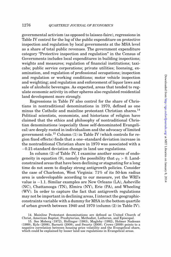
governmental activism (as opposed to laissez-faire), regressions inTable IV control for the log of the public expenditure on protectiveinspection and regulation by local governments at the MSA levelas a share of total public revenues. The government expenditurecategory “Protective inspection and regulation” in the Census ofGovernments includes local expenditures in building inspections;weights and measures; regulation of financial institutions; taxi-cabs; public service corporations; private utilities; licensing, ex-amination, and regulation of professional occupations; inspectionand regulation or working conditions; motor vehicle inspectionand weighting; and regulation and enforcement of liquor laws andsale of alcoholic beverages. As expected, areas that tended to reg-ulate economic activity in other spheres also regulated residentialland development more strongly.

Regressions in Table IV also control for the share of Chris-tians in nontraditional denominations in 1970, defined as oneminus the Catholic and mainline protestant Christian shares.14

Political scientists, economists, and historians of religion haveclaimed that the ethics and philosophy of nontraditional Chris-tian denominations (especially those self-denominated Evangeli-cal) are deeply rooted in individualism and the advocacy of limitedgovernment role.15 Column (1) in Table IV (which controls for re-gion fixed effects) finds that a one–standard deviation increase inthe nontraditional Christian share in 1970 was associated with a−0.21-standard deviation change in land use regulations.

In column (2) of Table IV, I examine another source of endo-geneity in equation (9), namely the possibility that ϕ2 > 0. Land-constrained areas that have been declining or stagnating for a longtime do not seem to display strong antigrowth policies. Considerthe case of Charleston, West Virginia: 71% of its 50-km radiusarea is undevelopable according to our measure, yet the WRI’svalue is −1.1. Similar examples are New Orleans (LA), Asheville(NC), Chattanooga (TN), Elmira (NY), Erie (PA), and Wheeling(WV). In order to capture the fact that antigrowth regulationsmay not be important in declining areas, I interact the geographic-constraints variable with a dummy for MSA in the bottom quartileof urban growth between 1940 and 1970 (column (2) in Table IV).

14. Mainline Protestant denominations are defined as United Church ofChrist, American Baptist, Presbyterian, Methodist, Lutheran, and Episcopal.

15. See Moberg (1972), Hollinger (1983), Magleby (1992), Holmer Nadesan(1999), Kyle (2006), Barnett (2008), and Swartz (2008). Crowe (2009) points to anegative correlation between housing price volatility and the Evangelical share,which could be explained by looser land use regulations in Evangelical areas.

at MIT



ownloaded from




TA

BL

EIV

EN

DO

GE

NE

ITY

OF

LA

ND

US

ER

EG

UL

AT

ION

S

Log

WR

I

(1)

(2)

(3)

(4)

Un

avai

labl

ela

nd,

50-k

mra

diu

s0.

134

−0.1

74−0

.241

(0.0

67)∗

∗(0

.125

)(0

.132

)∗U

nav

aila

ble

lan

din

grow

ing

citi

es(1

940–

1970

)0.

165

(0.0

69)∗

∗U

nav

aila

ble

lan

din

decl

inin

gci

ties

(194

0–19

70)

−0.0

54(0

.153

)D

ecli

nin

gci

ties

dum

my

(194

0–19

70)

−0.0

76(0

.051

)U

nav

aila

ble

lan

d,50

-km

radi

us

×0.

451

0.37

5�

log

hou

sin

gu

nit

s(1

970–

2000

)(0

.158

)∗∗∗

(0.1

54)∗

∗�

Log

hou

sin

gpr

ice

(197

0–20

00)=

log

hou

sin

gpr

ice

(197

0)0.

198

(0.0

88)∗

∗L

og(i

nsp

ecti

onex

pen

ditu

res/

loca

ltax

reve

nu

es)

(198

2)0.

051

0.04

70.

051

0.04

1(0

.015

)∗∗∗

(0.0

15)∗

∗∗(0

.015

)∗∗∗

(0.0

15)∗

∗∗S

har

eof

Ch

rist

ian

“non

trad

itio

nal

”de

nom

inat

ion

s(1

970)

−0.3

08−0

.304

−0.3

14−0

.291

(0.0

86)∗

∗∗(0

.084

)∗∗∗

(0.0

84)∗

∗∗(0

.090

)∗∗∗

Sh

are

wit

hba

chel

or’s

degr

eein

1970

0.98

30.

538

0.86

70.

089

(0.3

32)∗

∗∗(0

.342

)(0

.328

)∗∗∗

(0.4

04)

Non

-His

pan

icw

hit

esh

are

in19

800.

036

0.08

−0.0

69−0

.017

(0.1

13)

(0.1

10)

(0.1

16)

(0.1

20)

at MIT



ownloaded from




TA

BL

EIV

( CO

NT

INU

ED

)

Log

WR

I

(1)

(2)

(3)

(4)

Mid

wes

t−0

.266

−0.3

07−0

.289

−0.2

66(0

.039

)∗∗∗

(0.0

39)∗

∗∗(0

.039

)∗∗∗

(0.0

44)∗

∗∗S

outh

−0.1

9−0

.222

−0.2

61−0

.196

(0.0

54)∗

∗∗(0

.053

)∗∗∗

(0.0

58)∗

∗∗(0

.066

)∗∗∗

Wes

t−0

.029

−0.0

8−0

.096

−0.0

88(0

.050

)(0

.050

)(0

.054

)∗(0

.056

)C

onst

ant

1.42

51.

471

1.57

8−0

.759

(0.1

37)∗

∗∗(0

.135

)∗∗∗

(0.1

44)∗

∗∗(1

.055

)O

bser

vati

ons

269

269

269

269

R2

.43

.46

——

Met

hod

FG

LS

FG

LS

2SL

S3S

LS

Not

es.

Sta

nda

rder

rors

inpa

ren

thes

es.

Th

ede

pen

den

tva

riab

lein

all

regr

essi

ons

isth

elo

gof

the

WR

Ifo

rea

chm

etro

area

.T

ode

alw

ith

het

erog

eneo

us

sam

ple

size

s(s

tron

gco

rrel

atio

nof

WR

Iva

lues

wit

hin

MS

A)

colu

mn

s(1

)an

d(2

)u

sea

Fea

sibl

eG

ener

aliz

edL

east

Squ

ares

(FG

LS

)pr

oced

ure

,w

her

eea

chob

serv

atio

nis

wei

ghte

dpr

opor

tion

ally

toth

ein

vers

eof

the

squ

are

erro

rof

OL

Ses

tim

ates

(wh

ich

are

actu

ally

alw

ays

very

clos

ein

mag

nit

ude

and

sign

ifica

nce

).In

colu

mn

s(3

)an

d(4

),ch

ange

sin

the

log

oflo

cal

hou

sin

gpr

ices

and

quan

titi

esar

ein

stru

men

ted

usi

ng

the

dem

and

shoc

ksin

Tab

leII

I(i

ndu

stry

shif

t-sh

are,

hou

rsof

sun

,an

dim

mig

ran

tsh

ocks

),pl

us

the

lan

du

nav

aila

bili

tyva

riab

le.∗

sign

ifica

nt

at10

%;∗

∗ sig

nifi

can

tat

5%;∗

∗∗si

gnifi

can

tat

1%.

at MIT



ownloaded from




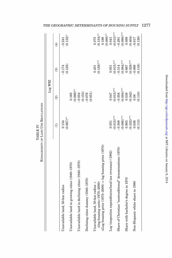
Lagged growth rates in a period that is, on the average, 45 yearsin the past are unlikely to be caused by the regulation environ-ment in 2005. But they are likely to be good predictors of futuregrowth, because of the permanence of factors that drove produc-tivity during the second half of the 20th century, such as relianceon manufacturing or mining or relative scarcity of institutions ofhigher education. Similarly, in column (3) of Table IV, I interactthe change in housing growth between 1970 and 2000 with thegeographic land-unavailability variable. Of course, housing con-struction is endogenous to regulations in this equation. HenceI use the demand shock instruments in Table III and interac-tions with geographic land unavailability as instrumental vari-ables for the interacted endogenous variable. The results suggestthat regulations are stricter in land-constrained metro areas thatare thriving (ϕ2 > 0). In declining cities, however, regulations areinsensitive to previous factors that made housing supply inelastic.

Finally, in column (4) of Table IV, I test for reverse causationfrom price levels to higher regulation (ϕ3 > 0 in equation (9)). Be-cause Pt = �Pt,t−n + Pt−n, I express the log of housing values in2000 as the sum of the change in the log of prices plus the log of ini-tial prices in 1970 (for comparability with Table III) and constrainthe coefficient on both variables to be the same.16 The instrumentsnow are hours of sun, immigration shocks, and the Bartik (1991)employment shift-share and their interactions with geographicland unavailability. There are two endogenous variables: laggedchanges in housing prices, and household growth interacted by thegeographic constraints. The equation is estimated via 3SLS andstrongly suggests that both a constraining geography in growingcities and higher housing prices led to a more regulated supplyenvironment circa 2005.

In sum, the regulation equations in Table IV demonstratethat higher housing prices, demographic growth, and natural con-straints beget more restrictive land-use regulations.

V.B. Endogeneizing Regulations in the Supply Equation

Because regulations are endogenous to εk in equations (5) and(6), one needs to use additional identifying exclusions to estimatehousing supply elasticities. As suggested by the results in TableIV, the local public expenditure share in protective inspection and

16. In unconstrained equations, I cannot reject that the separate coefficientson �P2000,1970 and P1970 are statistically equivalent.

at MIT



ownloaded from




the nontraditional Christian share in 1970 can be used as instru-ments for the 2005 WRI: although they predict land use regu-lations, they are unlikely to impact land supply otherwise (notethat the supply equation controls for the evolution of constructioncosts). As seen in Table IV, these variables prove also to be stronginstruments.17 Note that even if these variables were correlatedwith demand shocks, the regression have more supply-specific ex-clusion restrictions than endogenous variables and all parametersare fully identified. In fact, because the two endogenous variablesappear in interacted form, I can now also include in the IV listthe interactions of the instruments used for changes in quantities(hours of sun, employment shift-share, and immigration shocks)with those used for the regulation index (municipal inspectionsexpenditure share and nontraditional Christian share). Impor-tantly, the results are very similar when I simply use each one ofthe regulation instruments separately.

Column (1) in Table V reestimates the specification in Ta-ble III, column (5) (elasticities as linear functions of regulationsand geographic constraints), this time allowing for endogenousregulations. The coefficient on the WRI declines to about 60%of its previous value. However, when the model in equation (6)is reestimated (land constraints matter more in large cities),the coefficient on the regulation index takes a value that is only8% smaller than in the earlier estimates. Therefore, parametersfrom previous research are bound to somewhat overestimatethe impact of regulations on prices, but it is still true that moreregulated areas tend to be relatively more inelastic, and thisimpact is quantitatively large. In Table V, column (2), a moveacross the interquartile range in the WRI of a city of one millioninhabitants with average land availability is associated withclose to a 20% reduction in supply elasticity: from 1.76 to 1.38.

The impact of constrained geography is larger, especially inlarger cities. For example, in a metro area with average regula-tions and a population of one million, the interquartile change inthe share of unavailable land (from 0.09 to 0.38) implies a 50%reduction in supply elasticity (from 2.45 to 1.25).

In a separate Online Appendix, the interested reader canfurther see that endogeneizing construction costs (which could bethemselves a function of geography) and immigration shocks doesnot change the main parameters of interest.

17. Partial R2 of .074 in the first stage and F-test of 10.413, above the 20%maximal bias threshold (8.75) in Stock and Yogo (2005).

at MIT



ownloaded from




TABLE VHOUSING SUPPLY: ENDOGENOUS REGULATIONS

�log(P) (supply)

(1) (2)

Unavailable land ×�log(Q) 0.581 −5.260(0.119)∗∗∗ (1.396)∗∗∗

Log(1970 population) × unavailable 0.475land ×�log(Q) (0.119)∗∗∗

Log(WRI) ×�log(Q) 0.109 0.280(0.078)∗ (0.077)∗∗∗

Midwest −0.009 0.002(0.049) (0.048)

South −0.075 −0.109(0.049) (0.049)∗∗

West 0.149 0.059(0.063) (0.065)

Constant 0.659 0.577(0.048)∗∗∗ (0.048)∗∗∗

Notes. Standard errors in parentheses. The table shows the coefficient of 2SLS estimation of a metropoli-tan housing supply equation. The specification and instruments used for demand shocks are as in Table III.Demand shocks are interacted with the unavailable land share (due to geography) and the log of the WRI. Thelatter variable is treated as endogenous using the share of local public expenditures on “protective inspections”and the share of nontraditional Christian denominations as instruments. Because we are instrumenting forlog(WRI)×� log(Q), I also include the interaction between the regulation and the demand instruments in theIV list. ∗significant at 10%; ∗∗significant at 5%; ∗∗∗significant at 1%.

V.C. Estimated Elasticities

In this section, I use the coefficients in Table V, column (2),to estimate supply elasticities at the metro area level. Such esti-mates are simple nonlinear combinations of the available data onphysical and regulatory constraints, and predetermined popula-tion levels in 2000. These elasticities are thus based on economicfundamentals related to natural and man-made land constraintsand should prove useful in calibrating general equilibrium modelsof interregional labor mobility and in predicting the response ofhousing markets to future demand shocks.

The population-weighted average elasticity of supply is esti-mated to be 1.75 in metropolitan areas (2.5 unweighted). The re-sults for metropolitan areas with population over 500,000 in 2000can be found in Table VI. Estimated elasticities using only the ge-ographic, regulatory, and initial population variables agree withperceptions about supply-constrained areas. Miami, Los Angeles,San Francisco, Oakland, New York, San Diego, Boston, Chicago,

at MIT



ownloaded from




and Seattle are among the top fifteen in the list of the most in-elastic cities. Houston, Austin, Charlotte, Kansas City, and In-dianapolis are among the large metro areas with highly elastichousing supply.

Estimated elasticities (this time using predetermined 1970population in order to avoid obvious endogeneity issues) also cor-relate very strongly with housing price levels in 2000 and changesover the 1970–2000 period. Figure II presents plots relating hous-ing prices (Panel 1) or changes (Panel 2) on the vertical axis andthe inverse of the estimated supply elasticity by metropolitan areaon the horizontal axis. It is clear that a simple linear combinationof physical and regulatory constraints goes very far to explain theevolution of prices, even without taking into account the differen-tial demand shocks that cities experienced.

VI. CONCLUSION

The paper started by providing empirical content to the con-cept of land availability in metropolitan areas. Using satellite-generated data, I calculated an exact measure of land unavailablefor real estate development in the metropolitan United States.This geographic measure can be used in future work exploringtopics as diverse as housing and mortgage markets, labor mobility,urban density, transportation, and urban environmental issues.

I then developed a model for the impact of land availabilityon urban development and housing prices. In ex post equilibrium,land-constrained metro areas should have more expensive hous-ing and enjoy higher amenities or productivity, as confirmed bythe data. The model demonstrates that land constraints shouldalso decrease housing supply elasticities, a somewhat ad hoc as-sumption in previous literature.

Empirically, most areas that are widely regarded as supply-inelastic were found, in fact, to be severely land-constrained bytheir geography. Deploying a new comprehensive survey on resi-dential land use regulations, I found that highly regulated areastend to be geographically constrained also. More generally, I foundrecent housing price and population growth to be predictive ofmore restrictive residential land regulations. The results point tothe endogeneity of land use controls with respect to the housingmarket equilibrium.

Hence I next estimated a model where regulations are bothcauses and consequences of housing supply inelasticity. Housing

at MIT



ownloaded from



THE GEOGRAPHIC DETERMINANTS OF HOUSING SUPPLY 1283T

AB

LE

VI

SU

PP

LYE

LA

ST

ICIT

IES

(ME

TR

OA

RE

AS

WIT

HP

OP

UL

AT

ION

>50

0,00

0)

Ran

kM

SA

/NE

CM

An

ame

Su

pply

elas

tici

tyR

ank

MS

A/N

EC

MA

nam

eS

upp

lyel

asti

city

1M

iam

i,F

L0.

6026

Val

lejo

–Fai

rfiel

d–N

apa,

CA

1.14

2L

osA

nge

les–

Lon

gB

each

,CA

0.63

27N

ewar

k,N

J1.

163

For

tL

aude

rdal

e,F

L0.

6528

Ch

arle

ston

–Nor

thC

har

lest

on,S

C1.

204

San

Fra

nci

sco,

CA

0.66

29P

itts

burg

h,P

A1.

205

San

Die

go,C

A0.

6730

Tac

oma,

WA

1.21

6O

akla

nd,

CA

0.70

31B

alti

mor

e,M

D1.

237

Sal

tL

ake

Cit

y–O

gden

,UT

0.75

32D

etro

it,M

I1.

248

Ven

tura

,CA

0.75

33L

asV

egas

,NV

–AZ

1.39

9N

ewY

ork,

NY

0.76

34R

och

este

r,N

Y1.

4010

San

Jose

,CA

0.76

35T

ucs

on,A

Z1.

4211

New

Orl

ean

s,L

A0.

8136

Kn

oxvi

lle,

TN

1.42

12C

hic

ago,

IL0.

8137

Jers

eyC

ity,

NJ

1.44

13N

orfo

lk–V

irgi

nia

Bea

ch–N

ewpo

rt0.

8238

Min

nea

poli

s–S

t.P

aul,

MN

–WI

1.45

New

s,V

A–N

C14

Wes

tP

alm

Bea

ch–B

oca

Rat

on,F

L0.

8339

Har

tfor

d,C

T1.

5015

Bos

ton

–Wor

cest

er–L

awre

nce

–Low

ell–

0.86

40S

prin

gfiel

d,M

A1.

52B

rock

ton

,MA

–NH

16S

eatt

le–B

elle

vue–

Eve

rett

,WA

0.88

41D

enve

r,C

O1.

5317

Sar

asot

a–B

rade

nto

n,F

L0.

9242

Pro

vide

nce

–War

wic

k–P

awtu

cket

,RI

1.61

18R

iver

side

–San

Ber

nar

din

o,C

A0.

9443

Was

hin

gton

,DC

–MD

–VA

–WV

1.61

19N

ewH

aven

–Bri

dgep

ort–

Sta

mfo

rd–

0.98

44P

hoe

nix

–Mes

a,A

Z1.

61D

anbu

ry–W

ater

bury

,CT

20T

ampa

–St.

Pet

ersb

urg

–Cle

arw

ater

,FL

1.00

45S

cran

ton

–Wil

kes-

Bar

re–H

azle

ton

,PA

1.62

21C

leve

lan

d–L

orai

n–E

lyri

a,O

H1.

0246

Har

risb

urg

–Leb

anon

–Car

lisl

e,P

A1.

6322

Mil

wau

kee–

Wau

kesh

a,W

I1.

0347

Bak

ersfi

eld,

CA

1.64

23Ja

ckso

nvi

lle,

FL

1.06

48P

hil

adel

phia

,PA

–NJ

1.65

24P

ortl

and–

Van

cou

ver,

OR

–WA

1.07

49C

olor

ado

Spr

ings

,CO

1.67

25O

rlan

do,F

L1.

1250

Alb

any–

Sch

enec

tady

–Tro

y,N

Y1.

70

at MIT



ownloaded from



1284 QUARTERLY JOURNAL OF ECONOMICST

AB

LE

VI

( CO

NT

INU

ED

)

Ran

kM

SA

/NE

CM

An

ame

Su

pply

elas

tici

tyR

ank

MS

A/N

EC

MA

nam

eS

upp

lyel

asti

city

51G

ary,

IN1.

7474

Atl

anta

,GA

2.55

52B

aton

Rou

ge,L

A1.

7475

Akr

on,O

H2.

5953

Mem

phis

,TN

–AR

–MS

1.76

76R

ich

mon

d–P

eter

sbu

rg,V

A2.

6054

Bu

ffal

o–N

iaga

raF

alls

,NY

1.83

77Y

oun

gsto

wn

–War

ren

,OH

2.63

55F

resn

o,C

A1.

8478

Col

um

bia,

SC

2.64

56A

llen

tow

n–B

eth

leh

em–E

asto

n,P

A1.

8679

Col

um

bus,

OH

2.71

57W

ilm

ingt

on–N

ewar

k,D

E–M

D1.

9980

Gre

envi

lle–

Spa

rtan

burg

–An

ders

on,S

C2.

7158

Mob

ile,

AL

2.04

81L

ittl

eR

ock–

Nor

thL

ittl

eR

ock,

AR

2.79

59S

tock

ton

–Lod

i,C

A2.

0782

For

tW

orth

–Arl

ingt

on,T

X2.

8060

Ral

eigh

–Du

rham

–Ch

apel

Hil

l,N

C2.

1183

San

An

ton

io,T

X2.

9861

Alb

uqu

erqu

e,N

M2.

1184

Au

stin

–San

Mar

cos,

TX

3.00

62B

irm

ingh

am,A

L2.

1485

Ch

arlo

tte–

Gas

ton

ia–R

ock

Hil

l,N

C–S

C3.

0963

Dal

las,

TX

2.18

86G

reen

sbor

o–W

inst

on–S

alem

–Hig

hP

oin

t,N

C3.

1064

Syr

acu

se,N

Y2.

2187

Kan

sas

Cit

y,M

O–K

S3.

1965

Tol

edo,

OH

2.21

88O

klah

oma

Cit

y,O

K3.

2966

Nas

hvi

lle,

TN

2.24

89T

uls

a,O

K3.

3567

An

nA

rbor

,MI

2.29

90O

mah

a,N

E–I

A3.

4768

Hou

ston

,TX

2.30

91M

cAll

en–E

din

burg

–Mis

sion

,TX

3.68

69L

ouis

vill

e,K

Y–IN

2.34

92D

ayto

n–S

prin

gfiel

d,O

H3.

7170

ElP

aso,

TX

2.35

93In

dian

apol

is,I

N4.

0071

St.

Lou

is,M

O–I

L2.

3694

For

tW

ayn

e,IN

5.36

72G

ran

dR

apid

s–M

usk

egon

–Hol

lan

d,M

I2.

3995

Wic

hit

a,K

S5.

4573

Cin

cin

nat

i,O

H–K

Y–IN

2.46

at MIT



ownloaded from




11

11.5

12

12.5

13

0 .5 1 1.5 2Inverse of supply elasticity

Log median house value Fitted values

1.5

2

2.5

3

0 .5 1 1.5 2Inverse of supply elasticity

Log price 2000 – log price 1970 Fitted values

(a)

(b)

FIGURE IIEstimated Elasticities and Home Values (2000)

(a) Levels, (b) changes.

at MIT



ownloaded from




demand, construction, and regulations are all determined en-dogenously. Housing supply elasticities were found to be wellcharacterized as functions of both physical and regulatory landconstraints, which in turn are endogenous to prices and pastgrowth.

Geography was shown to be one of the most important de-terminants of housing supply inelasticity: directly, via reductionsin the amount of land availability, and indirectly, via increasedland values and higher incentives for antigrowth regulations.The results in the paper demonstrate that geography is a keyfactor in the contemporaneous urban development of the UnitedStates, and help us understand why robust national demographicgrowth and increased urbanization has translated mostly intohigher housing prices in San Diego, New York, Boston, and LosAngeles, but into rapidly growing populations in Atlanta, Phoenix,Houston, and Charlotte.

APPENDIX IDESCRIPTIVE STATISTICS

Mean(standard dev.)

Log population in 2000 12.893(1.060)

Log median house value in 2000 11.592(0.342)

�log median house value (1970–2000) 1.937(0.213)

Log income in 2000 10.200(0.184)

�log(income per capita) (1990–2000) 0.401(0.063)

Log population (1990–2000) 0.123(0.099)

Immigrants (1990–2000)/population (2000) 0.034(0.038)

Share with bachelor’s degree (2000) 0.198(0.063)

Share workers in manufacturing (2000) 0.174(0.071)

Log(patents/population) (2000) −8.978(0.866)

January monthly hours of sun (average 1941–1970) 151.342(38.199)

Log tourist visits per person (2000) −12.679(0.830)

at MIT



ownloaded from




APPENDIX I(CONTINUED)

Mean(standard dev.)

Ocean dummy 0.331(0.471)

Unavailable land, 50-km radius 0.261(0.212)

Log(WRI) 1.025(0.278)

�log housing units (1970–2000) 0.599(0.319)

Log housing price (1970) 9.655(0.228)

Log (inspection expenditures/local tax revenues) −5.826(0.971)

Share of Christian “nontraditional” denominations 0.351(0.209)

Share with bachelors degree in 1970 0.111(0.042)

Non-Hispanic white share in 1980 0.827(0.138)

Midwest 0.264(0.442)

South 0.383(0.487)

West 0.201(0.401)

Unionization in construction sector 0.208(0.146)

�log(income per capita) (1970–2000) 1.965(0.116)

APPENDIX II: DERIVATIONS AND PROOFS

Derivation 1. First, note that a share of 2πd�k/γ POPk

households live in the sector of the circle at a distance d from theCBD. Average housing rents in the city, conditional on population,can thus be obtained as rk = ∫ �k

0 (2πx�k/γ POPk) · r(x) · dx, whichimplies that rk = (2π�k/γ POPk)

∫ �k

0 (r0x − tx2)dx, and so rk =(2π�k/γ POPk) · [ 1

2r0x2 − 13 tx3]�k

0 . Therefore rk = (2π�k/γ POPk) ·[ 1

2r0�2k − 1

3 t�3k] = (�2

kπ�k/γ POPk) · [r0− 23 t�k] = {[(γ POPk/(�kπ )) ·

π�k]/γ POPk} · [r0 − 23 t�k] = [r0 − t 2

3�k], which corresponds torents in the location that is two-thirds of the way between the

at MIT



ownloaded from




CBD and the city’s fringe. Substituting for the value of r( 23�k)

yields rk = iCC + 13 t

√γ POPk/�kπ .

Derivation 2. Recall that

(10) U (Ck) = (Ak + wk − r − td)ρ = 0.

Substituting into the intercity spatial equilibrium equation,I obtain r(POPk, d) = Ak + wk − (ψ + α)

√POPk − td. Because all

consumers are indifferent, I can focus w.o.l.o.g. on consumersliving in the CBD. Recalling that Hk = POPk yields r0 = Ak +wk − (ψ + α)

√Hk. Defining P(0) = r0/i, one obtains the demand

schedule for housing in the city:

(11)√

Hk = Ak + wk

(ψ + α)− i

(ψ + α)P(0).

Note also that changes in P(0) shift all prices within a cityvertically by the same amount and so, denoting Pk as the averagehousing price in city k, the city demand equation implies that∂ ln(Hk)/∂ Pk = ∂ ln(Hk)/∂ P(0). Now recall the expression for rentsin the CBD from the supply of land: r0 = iCC + t

√γ Hk/�kπ, which

implies that P(0) = CC + ti

√γ Hk/�kπ .

I can combine this supply-side price equation at theCBD with equation (11) to obtain Ak + wk − (ψ + α)

√Hk = iCC +

t(√

γ /�kπ)√

Hk. Solving for housing yields

Hk =⎛⎝ Ak + wk − iCC

(ψ + α) + t√

γ

�kπ

⎞⎠2

.

Proof of Proposition 1. The city-specific inverse elastic-ity of supply is βS

k = ∂ ln Pk/∂ ln Hk = 12 [ 1

3i t(√

γ Hk/�kπ)/Pk], andtherefore

(12)∂βk

∂�k= ∂2 ln Pk

∂ ln Hk∂�k= −1

4

13i t

√γ Hk

�3kπ

CC

(Pk)2< 0.

Proof of Proposition 2. I focus on relevant joint amenityand productivity shocks net of annuitized construction costs thatare compatible with habitation: χk ≡ Ak + wk − iCC > 0. I fur-ther normalize the minimum city size that classifies a popula-tion center as metropolitan to one (POPk = Hk = 1). The unit

at MIT



ownloaded from




of population measurement could be, for instance, 50,000 peo-ple, which is the actual population level that qualifies an urbanarea for metropolitan status in the United States. The mini-mum necessary net wage–amenity shock observed in metropoli-tan areas (χ) is obtained with �k = 1 (all land is developable)and therefore χ = (ψ + α) + t

√γ /π . Similarly, I denote the

minimum amenity–productivity shock that a city with land avail-ability (� j) requires to reach metropolitan status as χ (� j) =χ + t

√γ /π [(1/

√� j) − 1]. Start by defining ε(� j) = χ (� j) − χ , to

obtain ε j = t√

γ /π [(1/√

� j) − 1]. By assumption, conditional onqualifying as a metropolitan area, amenity–productivity shocks inland-unconstrained cities (�k = 1) are drawn from the Pareto cdf:f (χ/χ ≥ χ, λ) = λχλ/χλ+1, with λ > 2. Thus the expected value ofshocks in such cities is E(χ/χ ≥ χ, λ) = λχ/(λ − 1).

In turn, amenity–productivity shocks in land-constrainedmetropolitan areas with � j < 1 will be drawn (ex post) from distri-butions with support [χ + ε(� j),∞]. The Pareto cdf implies thatF(χ + ε(� j)) = 1 − (χ/χ + ε(� j))λ, and so the upper tail truncatedat χ + ε(� j) has mass (χ/χ + ε(� j))λ. Therefore

f (χ/χ ≥ χ + ε(� j)) = λχλ

χλ+1

/(χ

χ + ε(� j)

)λ

= λ(χ + ε(� j))λ/χλ+1,

which is itself Pareto distributed. Note that E(χ/χ ≥ χ +ε(� j)) = E(χ/POP j ≥ 1� j), and therefore E(χ/POP j ≥ 1,� j) =λ[χ + ε j(� j)]/[λ − 1], which is a decreasing function in land avail-ability.

Proof of Proposition 3. Recall that POPk = {(χk/[(ψ + α) +t√

γ

�kπ)}2. Using the relevant pdf:

E(POP j/POP j ≥ 1,� j)

=∫ ∞

χ+ε j (� j )

λ[χ + ε j(� j)]λ

zλ+1·⎛⎝ z

(ψ + α) + t√

γ

�kπ

⎞⎠2

dz,

at MIT



ownloaded from




E(POP j/POP j ≥ 1,� j)

=⎛⎝ 1

(ψ + α) + t√

γ

�kπ

⎞⎠2 ∫ ∞

χ+ε j (� j )λ[χ + ε j(� j)]λ · z1−λ · dz,

E(POP j/, POP j ≥ 1,� j)

=⎛⎝ 1

(ψ + α) + t√

γ

�kπ

⎞⎠2 [λ

2 − λ· (χ + ε j(� j))λ · z2−λ

]∞

χ+ε j (� j )

=⎛⎝ 1

(ψ + α) + t√

γ

�kπ

⎞⎠2 (0 + λ

λ − 2· (χ + ε j(� j))λ

· (χ + ε j(� j))2−λ

)

=⎛⎝ 1

(ψ + α) + t√

γ

�kπ

⎞⎠2 (λ

λ − 2· (χ + ε j(� j))2

)

=⎛⎝ (χ + ε j(� j))

(ψ + α) + t√

γ

�kπ

⎞⎠2

λ

λ − 2.

Because the first part of the equation defines the minimumpopulation level normalized at one: E(POP j/POP j ≥ 1,� j) =λ/(λ − 2).

Derivation 3. Recall the equilibrium population level:

H∗k =

⎛⎝ χk

(ψ + α) + t√

γ

�kπ

⎞⎠2

.

Substituting back into the supply equation, we obtain the equilib-rium average price

P∗k = CC + 1

3it

√γ H∗

k

�kπ= CC + 1

3i· χk( (ψ+α)

√�kπ

t√

γ

) + 1.

at MIT



ownloaded from




Therefore changes in productivity–amenities imply

�P∗k = 1

3i· �χk( (ψ+α)

√�kπ

t√

γ

) + 1.

The expectation of changes in housing prices is therefore

E(�P∗k ) =

∫13i

· �χk( (ψ+α)√

�kπ

t√

γ

) + 1· f (�χk) · d�χk,

which, given the independence assumption of productivity shocks,implies that

E(�P∗

k

) = 13i

· E(�χk)( (ψ+α)√

�kπ

t√

γ

) + 1.

Now, we can demonstrate that

dE(�P∗

k

)d�k

= − 13i

· E(�χk)[( (ψ+α)√

�kπ

t√

γ

) + 1]2 · 1

2· (ψ + α)

√π

t√

γ· �

− 12

k < 0.

More importantly,

d2 E(�P∗

k

)(d�k)2

= + 13i

· E(�χk)[( (ψ+α)√

�kπ

t√

γ

) + 1]3 · 1

2· (ψ + α)2 π

t2γ· �

− 12

k

+ 13i

· E(�χk)[( (ψ+α)√

�kπ

t√

γ

) + 1]2 · 1

4· (ψ + α)

√π

t√

γ· �

− 32

k > 0.

Therefore the expected price change is a decreasing convex func-tion of land availability: wherever land availability is high ini-tially, further changes in land availability do not change expectedprice growth much. Conversely, in areas with initially low landavailability, further constraints on land development have greaterimpacts on future prices.

at MIT



ownloaded from




AP

PE

ND

IXII

ID

AT

AA

PP

EN

DIX

Var

iabl

eS

ourc

eN

otes

Lan

du

nav

aila

bili

tyC

alcu

late

dby

auth

orfr

omel

evat

ion

and

lan

du

seG

ISda

tafr

omU

SG

SW

har

ton

Reg

ula

tion

Inde

xG

you

rko,

Sai

z,an

dS

um

mer

s(2

008)

See

Dat

ase

ctio

nin

text

.D

ecli

nin

gm

etro

area

:195

0–19

70C

alcu

late

dby

auth

orfr

omda

tain

His

tori

cal

Cen

sus

Bro

wse

r—U

niv

ersi

tyof

Vir

gin

iaA

dum

my

that

take

sva

lue

1if

grow

this

inth

elo

wes

tqu

arti

leof

the

met

roar

eas

inou

rsa

mpl

e.N

on-H

ispa

nic

wh

ite

shar

e(1

970)

HU

DS

tate

ofth

eC

itie

sda

taba

se(f

rom

the

Cen

sus)

BA

/BS

shar

e(1

970)

HU

DS

tate

ofth

eC

itie

sda

taba

se(f

rom

the

Cen

sus)

For

eign

-bor

nsh

are

(197

0)H

UD

Sta

teof

the

Cit

ies

data

base

(fro

mth

eC

ensu

s)T

ouri

stvi

sits

per

pers

on(2

000)

Car

lin

oan

dS

aiz

(200

8)L

ogpa

ten

tspe

rca

pita

Gla

eser

and

Sai

z(2

004)

Imm

igra

tion

shoc

kH

UD

Sta

teof

the

Cit

ies

data

base

(fro

mth

eC

ensu

s)T

he

diff

eren

cein

the

nu

mbe

rof

fore

ign

-bor

nin

divi

dual

sbe

twee

n19

70an

d20

00,d

ivid

edby

the

met

roar

eapo

pula

tion

in19

70.

Sh

are

ofw

orke

rsin

man

ufa

ctu

rin

g(1

970)

HU

DS

tate

ofth

eC

itie

sda

taba

se(f

rom

the

Cen

sus)

Med

ian

hou

sin

gpr

ice

(197

0,20

00)

HU

DS

tate

ofth

eC

itie

sda

taba

se(f

rom

the

Cen

sus)

Nu

mbe

rof

hou

sin

gu

nit

s(1

970,

2000

)H

UD

Sta

teof

the

Cit

ies

data

base

(fro

mth

eC

ensu

s)P

erce

nta

geof

Ch

rist

ian

sin

“non

trad

itio

nal

”de

nom

inat

ion

s,19

71

Ch

urc

hes

and

chu

rch

mem

bers

hip

inth

eU

nit

edS

tate

s,19

71—

the

Ass

ocia

tion

ofR

elig

ion

data

arch

ives

Cal

cula

ted

ason

em

inu

sth

esh

are

ofC

ath

olic

Ch

urc

had

her

ents

and

mai

nli

ne

Pro

test

ants

(Un

ited

Ch

urc

hof

Ch

rist

,Am

eric

anB

apti

st,

Pre

sbyt

eria

n,M

eth

odis

t,L

uth

eran

,an

dE

pisc

opal

).%

voti

ng

for

Car

ter

(198

0)C

oun

tyan

dC

ity

Dat

aB

ook

1983

at MIT



ownloaded from



THE GEOGRAPHIC DETERMINANTS OF HOUSING SUPPLY 1293A

PP

EN

DIX

III

( CO

NT

INU

ED

)

Var

iabl

eS

ourc

eN

otes

Loc

alta

xre

ven

ues

(198

2)C

ensu

sof

Gov

ern

men

ts19

8220

00co

un

ty-b

ased

met

ropo

lita

nde

fin

itio

ns

wer

eu

sed

toag

greg

ate

atth

em

etro

leve

l.In

spec

tion

expe

ndi

ture

s/lo

cal

tax

reve

nu

es(1

982)

Cen

sus

ofG

over

nm

ents

1982

Coa

stal

met

roar

eadu

mm

yR

appa

port

and

Sac

hs

(200

3)A

dum

my

that

take

sva

lue

1if

the

min

imu

mdi

stan

cein

anM

SA

’sco

un

tyis

belo

w10

0km

.Ja

nu

ary

mon

thly

hou

rsof

sun

(ave

rage

1941

–197

0)N

atu

ralA

men

itie

sS

cale

—U

SD

AE

con

omic

Res

earc

hS

ervi

ceC

onst

ruct

ion

cost

s(s

ingl

e-fa

mil

y,av

erag

equ

alit

y)

Gyo

urk

oan

dS

aiz

(200

6)—

orig

inal

lyfr

omM

ean

set

al.

Hou

sin

gpr

ice

repe

atsa

les

inde

xF

redd

ieM

acpu

rch

ase-

only

con

ven

tion

alm

ortg

age

hom

epr

ice

inde

xL

and

valu

esh

ares

Dav

isan

dH

eath

cote

(200

7);D

avis

and

Pal

um

bo(2

008)

Dav

isan

dH

eath

cote

(200

7)ca

lcu

late

the

aver

age

shar

eof

lan

dfo

rre

side

nti

alre

ales

tate

inth

eU

nit

edS

tate

sin

1970

tobe

20%

.In

1984

(th

efi

rst

year

for

wh

ich

thei

rm

etro

poli

tan

data

seri

esis

avai

labl

e)D

avis

and

Pal

um

bo(2

008)

sugg

est

nat

ion

alan

dm

etro

poli

tan

lan

dsh

ares

tobe

very

sim

ilar

.We

ther

efor

ead

apt

anu

nw

eigh

ted

aver

age

20%

lan

dsh

are

acro

ssm

etro

poli

tan

area

sin

1970

.We

then

calc

ula

tedi

ffer

ence

sin

the

stru

ctu

reco

st/v

alu

era

tio

bydi

vidi

ng

the

aver

age

con

stru

ctio

nco

stin

1970

for

a2,

000

sq.f

t.h

ome

(th

eav

erag

eh

ome

size

)by

the

med

ian

hom

eva

lue

inea

chm

etro

area

.Th

efi

nal

met

ropo

lita

n-l

evel

esti

mat

eof

stru

ctu

rals

har

esin

1970

(αit

−1)

ispr

opor

tion

alto

the

afor

emen

tion

edra

tio,

and

such

that

its

un

wei

ghte

dm

ean

acro

ssm

etro

area

sis

80%

.C

entr

alci

tyar

eas

(197

0,20

00)

Cou

nty

and

Cit

yD

ata

Boo

ks19

72,

2002

at MIT



ownloaded from




THE WHARTON SCHOOL, UNIVERSITY OF PENNSYLVANIA

REFERENCES

Alonso, W., Location and Land Use (Cambridge, MA: Harvard University Press,1964).

Altonji, Joseph, and David Card, “The Effects of Immigration on the Labor Mar-ket Outcome of Less-Skilled Natives,” Princeton University, Department OfEconomics, Industrial Relations Section, Working Paper 636, 1989.

Barnett, Timothy, “Evangelicals and Economic Enlightment,” paper for the 2008Annual Conference of the American Political Science Association, 2008.

Bartik, Timothy, “Who Benefits from State and Local Economic Development Poli-cies?” W. E. Upjohn Institute For Employment Research, Kalamazoo, MI, 1991.

Breton, Albert, “Neighborhood Selection and Zoning,” in Issues In Urban PublicEconomics, Harold Hochman, ed. (Saarbrucken: Institute Internationale DeFinance Publique, 1973).

Brueckner, Jan K., “The Structure of Urban Equilibria: A Unified Treatment of theMuth–Mills Model,” in Handbook Of Regional And Urban Economics, VolumeII, E. S. Mills. ed. (Princeton, NJ: Elsevier, 1987).

Brueckner, Jan K., “Strategic Control of Growth in a System of Cities,” Journal ofPublic Economics, 57 (1995), 393–416.

Burchfield, Marcy, Henry G. Overman, Diego Puga, and Matthew A. Turner,“Causes of Sprawl: A Portrait from Space,” Quarterly Journal of Economics,121 (2006), 587–633.

Capozza, Dennis R., and Robert W. Helsley, “The Stochastic City,” Journal of UrbanEconomics, 28 (1990), 187–203.

Carlino, Jerry, and Albert Saiz, “Beautiful City: Leisure Amenities and Ur-ban Growth,” Federal Reserve Bank of Philadelphia Working Paper SSRN-1280157, 2008.

Combes, Pierre-Philippe, Gilles Duranton, Laurent Gobillon, and Sebastien Roux,“Estimating Agglomeration Economies with History, Geology, and Worker Ef-fects,” Groupement de Recherche en Economie Quantitative d’Aix-MarseilleWorking Paper, 2009.

Crowe, Christopher, “Irrational Exuberance in the U.S. Housing Market: WereEvangelicals Left Behind?” IMF Working Paper 09/57, 2009.

Davis, Morris, and Jonathan Heathcote, “The Price and Quantity of ResidentialLand in the United States,” Journal of Monetary Economics, 54 (2007), 2595–2620.

Davis, Morris, and Michael G. Palumbo, “The Price of Residential Land in LargeU.S. Cities,” Journal of Urban Economics, 63 (2008), 352–384.

Eeckout, Jan, “Gibrat’s Law for (All) Cities,” American Economic Review, 94 (2004),1429–1451.

Epple, Dennis, Thomas Romer, and Radu Filimon, “Community Development withEndogenous Land Use Controls,” Journal of Public Economics, 35 (1988), 133–162.

Fischel, William A., The Homevoter Hypothesis: How Home Values Influence LocalGovernment (Cambridge, MA: Harvard University Press, 2001).

Gabaix, Xavier, “Zipf ’s Law for Cities: An Explanation,” Quarterly Journal of Eco-nomics, 114 (1999), 739–767.

Glaeser, Edward, “Reinventing Boston: 1640–2003,” Journal of Economic Geogra-phy, 5 (2005a), 119–153.

——, “Urban Colossus: Why New York Is America’s Largest City,” Federal ReserveBank of New York Economic Policy Review, 11 (2005b), 7–24.

Glaeser, Edward, and Joseph Gyourko, “Housing Cycles.” NBER Working Paper12787, 2006.

Glaeser, Edward, Joseph Gyourko, and Raven Saks, “Why Have Housing PricesGone Up?” American Economic Review, 95 (2005a), 329–333.

——, “Why Is Manhattan So Expensive? Regulation and Rise in Housing Prices,”Journal of Law and Economics, 48 (2005b), 331–370.

——, “Urban Growth and Housing Supply,” Journal of Economic Geography, 6(2006), 71–89.

at MIT



ownloaded from




Glaeser, Edward L., Jed Kolko, and Albert Saiz, “Consumer City,” Journal of Eco-nomic Geography, 1 (2001), 27–50.

Glaeser, Edward, and Albert Saiz, “The Rise of the Skilled City,” Brookings–Wharton Papers on Urban Affairs, 1 (2004), 47–105.

Gyourko, Joseph, “Looking Back to Look Forward: What Can We Learn about Ur-ban Development from Philadelphia’s 350-Year History?” Brookings–WhartonPapers on Urban Affairs, 1 (2005), 1–58.

——, “Housing Supply,” Zell–Lurie Real Estate Center, The Wharton School, Uni-versity of Pennsylvania Working Paper, 2008.

Gyourko, Joseph, and Albert Saiz, “Construction Costs and the Supply of HousingStructure,” Journal of Regional Science, 46 (2006), 661–680.

Gyourko, Joseph, Albert Saiz, and Anita A. Summers, “A New Measure of the Lo-cal Regulatory Environment for Housing Markets: The Wharton ResidentialLand Use Regulatory Index,” Urban Studies, 45 (2008), 693–729.

Hamilton, Bruce W., “Zoning and Property Taxation in a System of Local Govern-ments,” Urban Studies, 12 (1975), 205–211.

——, “Capitalization of Intrajurisdictional Differences in Local Tax Prices,” Amer-ican Economic Review, 99 (1976), 743–753.

Hilber, Christian, and Frederic Robert-Nicaud, “Owners of Developed Land versusOwners of Undeveloped Land: Why Land Use Is More Constrained in the BayArea Than in Pittsburgh,” CEP Discussion Paper No. 760 (LSE), 2006.

Hollinger, Dennis P., Individualism and Social Ethics: An Evangelical Syncretism(Boston: University Press of America, 1983).

Holmer Nadesan, Majia, “The Discourses of Corporate Spiritualism and Evangel-ical Capitalism,” Management Communication Quarterly: MCQ, 13 (1999), 3–42.

Kahn, Matthew, “Demographic Change and the Demand for Environmental Reg-ulation,” Journal of Policy Analysis and Management, 21 (2002), 45–62.

Kiel, Katherine A., and Jeffrey E. Zabel, “The Accuracy of Owner-Provided HouseValues: The 1978–1991 American Housing Survey,” Real Estate Economics, 27(1999), 263–298.

Kyle, Richard G., Evangelicalism: An Americanized Christianity (New Brunswick,NJ: Transaction Publishers, 2006).

Magleby, Daniel B., “Political Behavior,” in The Encyclopedia of Mormonism, D.Ludlow, ed. (New York: Macmillan, 1992).

Malpezzi, Stephen, “Housing Prices, Externalities, and Regulation in U.S.Metropolitan Areas,” Journal of Housing Research, 7 (1996), 209–241.

Malpezzi, Stephen, Gregory H. Chun, and Richard K. Green, “New Place-to-PlaceHousing Price Indexes for U.S. Metropolitan Areas, and Their Determinants,”Real Estate Economics, 26 (1998), 235–274.

Mayer, Christopher J., and C. Tsuriel Somerville, “Residential Construction: Usingthe Urban Growth Model to Estimate Housing Supply,” Journal of UrbanEconomics, 48 (2000), 85–109.

Mills, Edwin, “An Aggregative Model of Resource Allocation in a MetropolitanArea,” American Economic Review, 57 (1967), 197–210.

Moberg, David O., The Great Reversal: Evangelism and Social Concern (Philadel-phia: Lippincott, 1972).

Muth, Richard, Cities and Housing (Chicago: University of Chicago Press, 1969).Ortalo-Magne, Francois, and Andrea Prat, “The Political Economy of Housing Sup-

ply: Homeowners, Workers, and Voters,” LSE: STICERD—Theoretical Eco-nomics Paper Series No. /2007/514, 2007.

Ottavianno, Gianmarco, and Giovanni Peri, “The Effects of Immigration on USWages and Rents: A General Equilibrium Approach,” CEPR Discussion Papers6551 (revised), 2007.

Pence, Karen M., and Brian Bucks, "Do Homeowners Know Their House Valuesand Mortgage Terms?" FEDS Working Paper No. 2006-03, 2006.

Quigley, John M., and Steven Raphael, “Regulation and the High Cost of Housingin California,” American Economic Review, 94 (2005), 323–328.

Rappaport, Jordan, “Moving to Nice Weather,” Regional Science and Urban Eco-nomics, 37 (2007), 375–398.

Rappaport, Jordan, and Jeffrey D. Sachs, “The United States as a Coastal Nation,”Journal of Economic Growth, 8 (2003), 5–46.

at MIT



ownloaded from




Rose, Louis A., “Topographical Constraints and Urban Land Supply Indexes,”Journal of Urban Economics, 26 (1989a), 335–347.

——, “Urban Land Supply: Natural and Contrived Reactions,” Journal of UrbanEconomics, 25 (1989b), 325–345.

Rosenthal, Stuart, and William C. Strange, “The Attenuation of Human CapitalSpillovers,” Journal of Urban Economics, 64 (2008), 373–389.

Rybczynski, Witold, Last Harvest: How a Cornfield Became New Daleville (Scrib-ner: New York, 2007).

Saiz, Albert, “Room in the Kitchen for the Melting Pot: Immigration and RentalPrices,” Review of Economics and Statistics, 85 (2003), 502–521.

——, “Immigration and Housing Rents in American Cities,” Journal of UrbanEconomics, 61 (2007), 345–371.

——, “On Local Housing Supply Elasticity,” The Wharton School, University ofPennsylvania Working Paper SSRN No. 1193422, 2008.

Saks, Raven, “Job Creation and Housing Construction: Constraints on Metropoli-tan Area Employment Growth,” Journal of Urban Economics, 64 (2008), 178–195.

Stock, James H., and Motohiro Yogo, “Testing for Weak Instruments in Linear IVRegression,” in Identification and Inference for Econometric Models: Essaysin Honor of Thomas Rothenberg, D. W. K. Andrews and J. H. Stock, eds.(Cambridge, UK: Cambridge University Press, 2005).

Swartz, David R., “Left Behind: The Evangelical Left and the Limits of EvangelicalPolitics: 1965–1988,” Ph.D. Dissertation, University of Notre Dame, 2008.

at MIT



ownloaded from



of housing supply - center for real estate housing supply ∗ albert saiz i ... a housing supply...

Documents