oceanic situational awareness over the pacific corridor · oceanic situational awareness over the...

Bryan Welch and Israel GreenfeldGlenn Research Center, Cleveland, Ohio

Oceanic Situational Awareness Overthe Pacific Corridor

NASA/TM—2005-213623

April 2005

https://ntrs.nasa.gov/search.jsp?R=20050175856 2018-06-24T05:01:18+00:00Z

The NASA STI Program Office . . . in Profile

Since its founding, NASA has been dedicated tothe advancement of aeronautics and spacescience. The NASA Scientific and TechnicalInformation (STI) Program Office plays a key partin helping NASA maintain this important role.

The NASA STI Program Office is operated byLangley Research Center, the Lead Center forNASA’s scientific and technical information. TheNASA STI Program Office provides access to theNASA STI Database, the largest collection ofaeronautical and space science STI in the world.The Program Office is also NASA’s institutionalmechanism for disseminating the results of itsresearch and development activities. These resultsare published by NASA in the NASA STI ReportSeries, which includes the following report types:

• TECHNICAL PUBLICATION. Reports ofcompleted research or a major significantphase of research that present the results ofNASA programs and include extensive dataor theoretical analysis. Includes compilationsof significant scientific and technical data andinformation deemed to be of continuingreference value. NASA’s counterpart of peer-reviewed formal professional papers buthas less stringent limitations on manuscriptlength and extent of graphic presentations.

• TECHNICAL MEMORANDUM. Scientificand technical findings that are preliminary orof specialized interest, e.g., quick releasereports, working papers, and bibliographiesthat contain minimal annotation. Does notcontain extensive analysis.

• CONTRACTOR REPORT. Scientific andtechnical findings by NASA-sponsoredcontractors and grantees.

• CONFERENCE PUBLICATION. Collectedpapers from scientific and technicalconferences, symposia, seminars, or othermeetings sponsored or cosponsored byNASA.

• SPECIAL PUBLICATION. Scientific,technical, or historical information fromNASA programs, projects, and missions,often concerned with subjects havingsubstantial public interest.

• TECHNICAL TRANSLATION. English-language translations of foreign scientificand technical material pertinent to NASA’smission.

Specialized services that complement the STIProgram Office’s diverse offerings includecreating custom thesauri, building customizeddatabases, organizing and publishing researchresults . . . even providing videos.

For more information about the NASA STIProgram Office, see the following:

• Access the NASA STI Program Home Pageat http://www.sti.nasa.gov

• E-mail your question via the Internet [email protected]

• Fax your question to the NASA AccessHelp Desk at 301–621–0134

• Telephone the NASA Access Help Desk at301–621–0390

• Write to: NASA Access Help Desk NASA Center for AeroSpace Information 7121 Standard Drive Hanover, MD 21076

Bryan Welch and Israel GreenfeldGlenn Research Center, Cleveland, Ohio

Oceanic Situational Awareness Overthe Pacific Corridor

NASA/TM—2005-213623

April 2005

National Aeronautics andSpace Administration

Glenn Research Center

Acknowledgments

The authors would like to acknowledge the assistance of Rafael Apaza, FAA, in obtaining historical Pacific Oceanflight data used in this analysis.

Available from

NASA Center for Aerospace Information7121 Standard DriveHanover, MD 21076

National Technical Information Service5285 Port Royal RoadSpringfield, VA 22100

Trade names or manufacturers’ names are used in this report foridentification only. This usage does not constitute an officialendorsement, either expressed or implied, by the National

Aeronautics and Space Administration.

This report contains preliminaryfindings, subject to revision as

analysis proceeds.

Available electronically at http://gltrs.grc.nasa.gov

NASA/TM—2005-213623 1

Oceanic Situational Awareness Over the Pacific Corridor

Bryan Welch and Israel Greenfeld National Aeronautics and Space Administration

Glenn Research Center Cleveland, Ohio 44135

Abstract

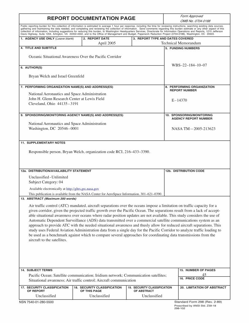
Air traffic control (ATC) mandated, aircraft separations over the oceans impose a limitation on traffic capacity for a given corridor, given the projected traffic growth over the Pacific Ocean. The separations result from a lack of acceptable situational awareness over oceans where radar position updates are not available. This study considers the use of Automatic Dependent Surveillance (ADS) data transmitted over a commercial satellite communications system as an approach to provide ATC with the needed situational awareness and thusly allow for reduced aircraft separations. This study uses Federal Aviation Administration data from a single day for the Pacific Corridor to analyze traffic loading to be used as a benchmark against which to compare several approaches for coordinating data transmissions from the aircraft to the satellites.

Introduction

Current procedures mandate that Pacific oceanic air traffic maintain 50 Nautical Mile (NMi) separations [1]. On the other hand, over Continental United States (CONUS) regions, Federal Aviation Administration (FAA) requires a 5 NMi separation. The difference in separation requirements is a direct result of the lack of surveillance radar coverage. Regularly derived position information from radar allows Air Traffic Control (ATC) to regularly monitor aircraft positions and react quickly to any changes. The very lack of surveillance radar over oceanic regions means that ATC does not have current position information, and therefore, must maintain much stricter separation requirements.

In the CONUS case where radar coverage is nearly ubiquitous, ATC radar data is automatically received at the regional control centers. Aircraft have little, if any, requirement to communicate nominal position information to ATC. Over the oceans, ATC must use High Frequency (HF) radio links to request position updates from each aircraft. HF radio has limitations in clarity and reliability. Additionally, HF communications are conducted through a third party. Direct controller-pilot communications are not possible which adds a time delay. HF radio does not mitigate the burden on ATC to obtain current position knowledge and therefore, the separation requirements cannot be relaxed.

This study explores the technical aspects of a satellite-based approach to oceanic aircraft surveillance that would provide ATC with more timely and reliable position information. This then may provide the means for reducing the current separation requirements and increasing oceanic corridor capacity. Specifically, by all aircraft in the Pacific Corridor having their Automatic Dependant Surveillance (ADS) data transmitted to an Aeronautical Mobile Satellite System (AMSS) and the AMSS relaying that data to ATC, the required surveillance information would be available to support reduced separations. The potential AMSS that is considered in this study is a Low-Earth Orbiting (LEO) satellite system, but another AMSS in geostationary can fulfill the role as well. The reason for choosing one particular AMSS is that it provides needed communication systems data for both the space and air segments.

It is noted that this study merely intends to investigate the broad technical aspects of ADS over satellite; that it is cognizant of, but is not applying in this study, the numerous, strict procedures imposed on oceanic crossing aircraft, in order to obtain a high level indication of what can be achieved just considering communications and geometry.

NASA/TM—2005-213623 2

Preliminary Considerations/Calculations

LEO Satellite Link As an example of a LEO satellite system, the Iridium system operates in the L-Band frequency and the link examined uses the Sensor Systems Inc. aircraft mounted antenna, S65-8282-401 [2]. The antenna has a minimum elevation angle of 8° with a gain of 0 dBic. The antenna produces 60 Watts (W) peak power which corresponds to an average power of 42.43 W. This specific antenna was modeled because it is representative of Iridium aircraft mounted antennas. Other link budget assumptions for the study are as follows:

• 3dB of Additional Losses • QPSK Modulation [3] • 1E-9 BER • Zenith Distance of 780 km [3] • Horizon Distance of 2460 km [3] • Frequency of 1.623 GHz • Iridium Satellite G/T of -16.315 dB/K • Burst Data Rate of 50 kbps [3]

The resulting link margins, table 1, for this case are shown below for both the zenith and horizon

distances in order to scope the link margin extremes. The horizon distance represents the worst case scenario when the satellite is at an elevation angle of 8°, at the edge of the satellite footprint in the outermost spot beam cells.

TABLE 1.—LINK MARGIN RESULTS

Scenario Zenith Horizon

Margin (dB) 11.52 1.55

As shown in table 1, sufficient margin exists to complete a link, assuming level flight, for the antenna

above 8° elevation angle.

Peak Traffic Baseline

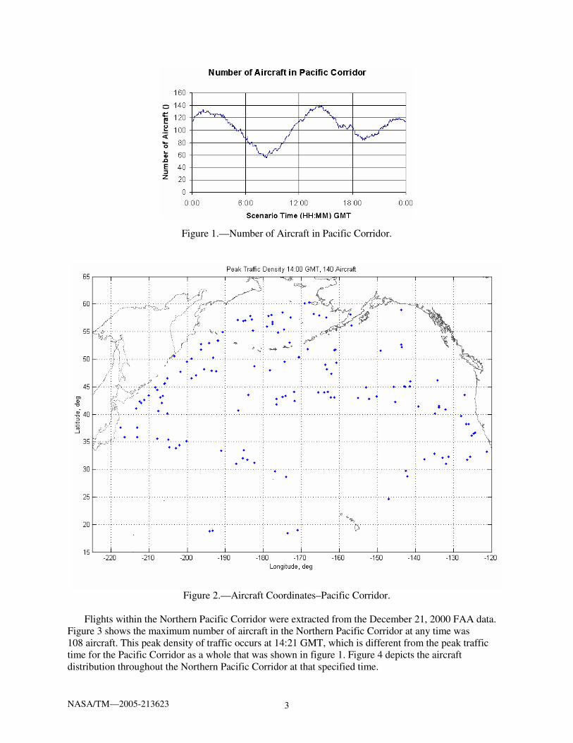
According to the FAA data, December 21, 2000 was the heaviest traffic day in the Pacific Corridor that year. Figure 1 shows that the maximum number of aircraft in the corridor at any time was 140. It is noted that the graph is bimodal corresponding to the surge of traffic first going west to east having a peak of 132 aircraft followed by the east to west surge having the 140 aircraft peak.

The peak of 140 aircraft shown in figure 1 occurs at 14:00 GMT. Figure 2 depicts the aircraft position distribution throughout the Pacific Corridor at that specified time.

Figure 2 shows that the Pacific Corridor contains three spatially separated sub-corridors. The remaining analysis for the Pacific Corridor will be broken down into these three separate sub-corridors as follows.

• Northern Pacific Corridor (Routes between California (through Alaska) and Asia) • Western Hawaiian Corridor (Routes between Hawaii and Asia) • Eastern Hawaiian Corridor (Routes between Hawaii and California)

NASA/TM—2005-213623 3

Figure 1.—Number of Aircraft in Pacific Corridor.

Figure 2.—Aircraft Coordinates–Pacific Corridor.

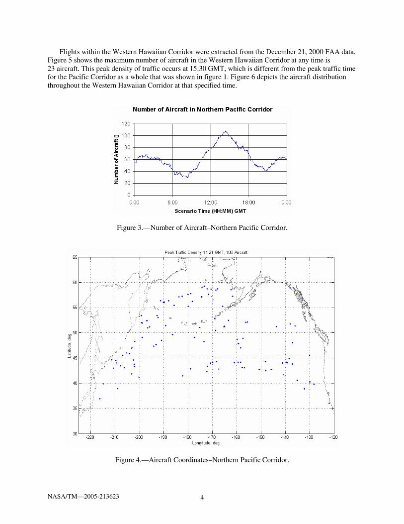
Flights within the Northern Pacific Corridor were extracted from the December 21, 2000 FAA data.

Figure 3 shows the maximum number of aircraft in the Northern Pacific Corridor at any time was 108 aircraft. This peak density of traffic occurs at 14:21 GMT, which is different from the peak traffic time for the Pacific Corridor as a whole that was shown in figure 1. Figure 4 depicts the aircraft distribution throughout the Northern Pacific Corridor at that specified time.

NASA/TM—2005-213623 4

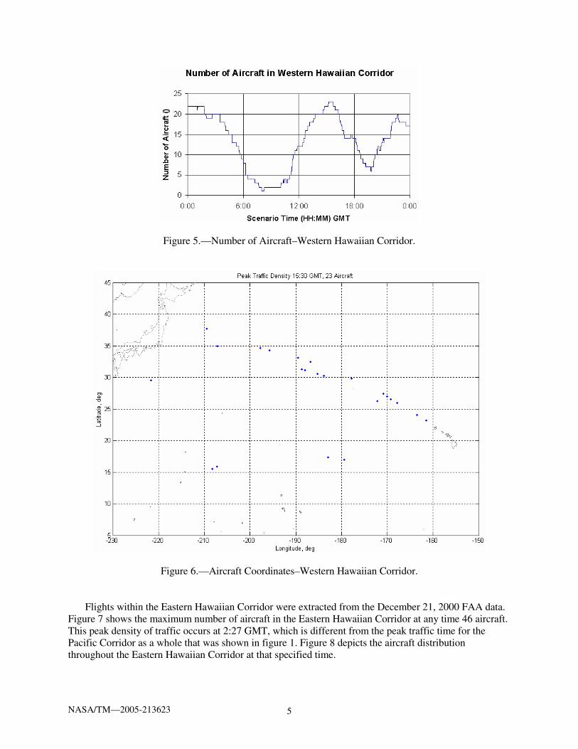
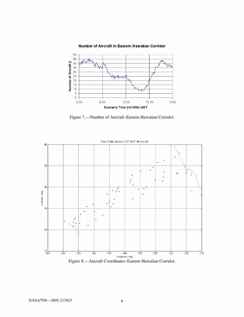
Flights within the Western Hawaiian Corridor were extracted from the December 21, 2000 FAA data. Figure 5 shows the maximum number of aircraft in the Western Hawaiian Corridor at any time is 23 aircraft. This peak density of traffic occurs at 15:30 GMT, which is different from the peak traffic time for the Pacific Corridor as a whole that was shown in figure 1. Figure 6 depicts the aircraft distribution throughout the Western Hawaiian Corridor at that specified time.

Figure 3.—Number of Aircraft–Northern Pacific Corridor.

Figure 4.—Aircraft Coordinates–Northern Pacific Corridor.

NASA/TM—2005-213623 5

Figure 5.—Number of Aircraft–Western Hawaiian Corridor.

Figure 6.—Aircraft Coordinates–Western Hawaiian Corridor.

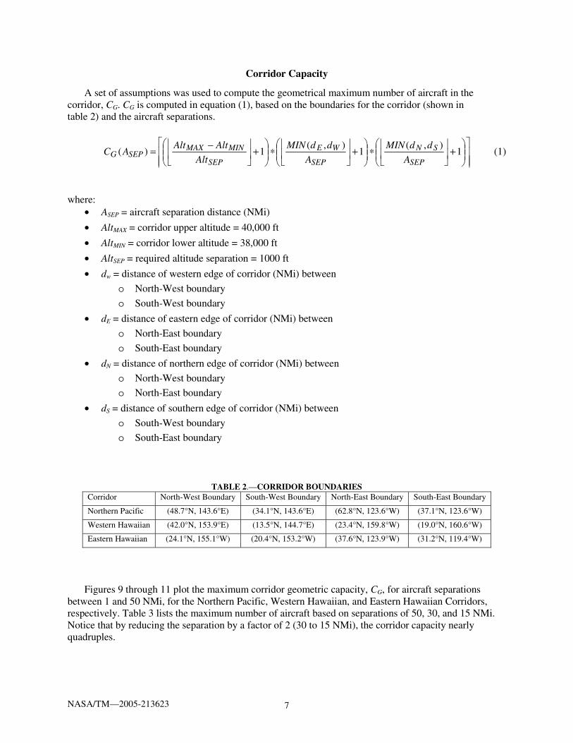
Flights within the Eastern Hawaiian Corridor were extracted from the December 21, 2000 FAA data. Figure 7 shows the maximum number of aircraft in the Eastern Hawaiian Corridor at any time 46 aircraft. This peak density of traffic occurs at 2:27 GMT, which is different from the peak traffic time for the Pacific Corridor as a whole that was shown in figure 1. Figure 8 depicts the aircraft distribution throughout the Eastern Hawaiian Corridor at that specified time.

NASA/TM—2005-213623 6

Figure 7.—Number of Aircraft–Eastern Hawaiian Corridor.

Figure 8.—Aircraft Coordinates–Eastern Hawaiian Corridor.

NASA/TM—2005-213623 7

Corridor Capacity

A set of assumptions was used to compute the geometrical maximum number of aircraft in the corridor, CG. CG is computed in equation (1), based on the boundaries for the corridor (shown in table 2) and the aircraft separations.

⎥⎥⎥

⎤

⎢⎢⎢

⎡⎟⎟⎠

⎞⎜⎜⎝

⎛+⎥

⎦

⎥⎢⎣

⎢∗⎟⎟⎠

⎞⎜⎜⎝

⎛+⎥

⎦

⎥⎢⎣

⎢∗⎟⎟⎠

⎞⎜⎜⎝

⎛+⎥

⎦

⎥⎢⎣

⎢ −= 1),(

1),(

1)(SEP

SN

SEP

WE

SEP

MINMAXSEPG

A

ddMIN

A

ddMIN

Alt

AltAltAC (1)

where:

• ASEP = aircraft separation distance (NMi)

• AltMAX = corridor upper altitude = 40,000 ft

• AltMIN = corridor lower altitude = 38,000 ft

• AltSEP = required altitude separation = 1000 ft

• dw = distance of western edge of corridor (NMi) between

o North-West boundary

o South-West boundary

• dE = distance of eastern edge of corridor (NMi) between

o North-East boundary

o South-East boundary

• dN = distance of northern edge of corridor (NMi) between

o North-West boundary

o North-East boundary

• dS = distance of southern edge of corridor (NMi) between

o South-West boundary

o South-East boundary

TABLE 2.—CORRIDOR BOUNDARIES Corridor North-West Boundary South-West Boundary North-East Boundary South-East Boundary

Northern Pacific (48.7°N, 143.6°E) (34.1°N, 143.6°E) (62.8°N, 123.6°W) (37.1°N, 123.6°W)

Western Hawaiian (42.0°N, 153.9°E) (13.5°N, 144.7°E) (23.4°N, 159.8°W) (19.0°N, 160.6°W)

Eastern Hawaiian (24.1°N, 155.1°W) (20.4°N, 153.2°W) (37.6°N, 123.9°W) (31.2°N, 119.4°W)

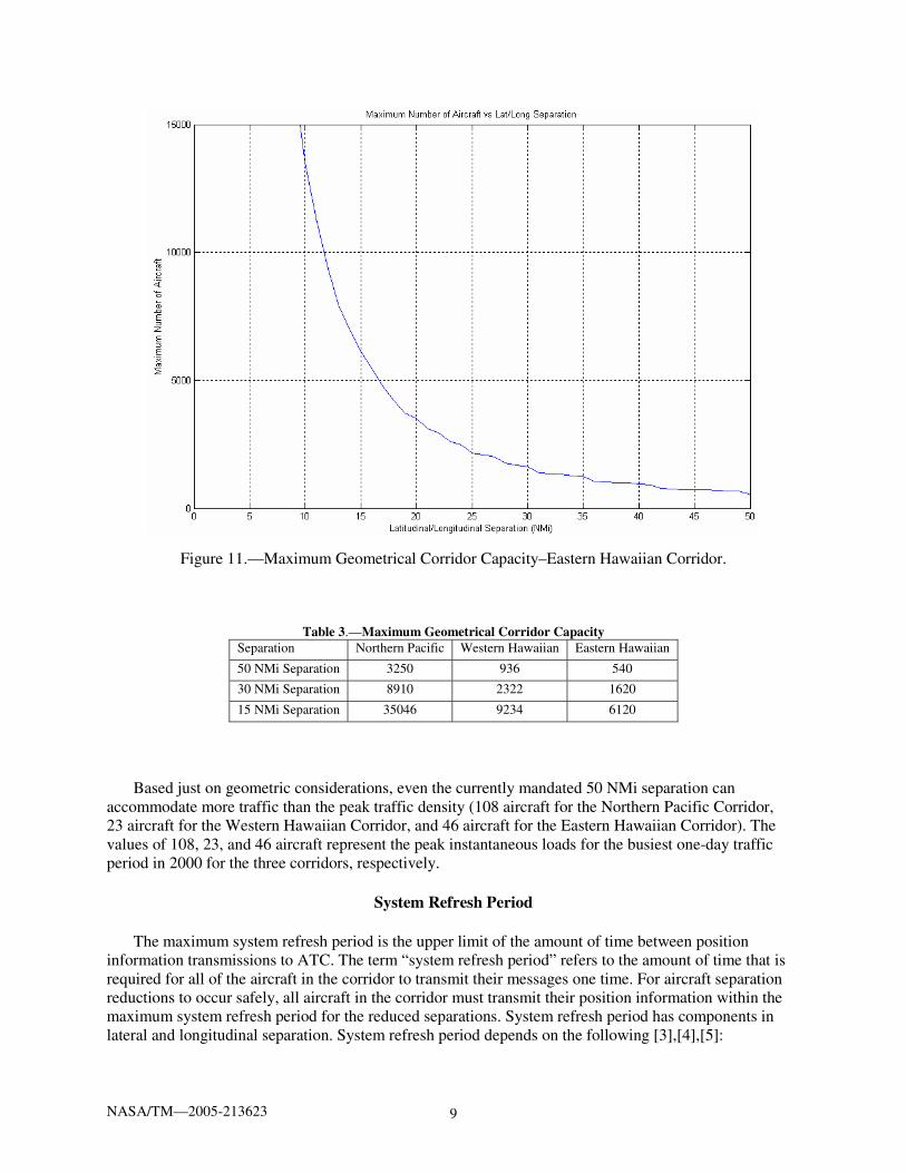
Figures 9 through 11 plot the maximum corridor geometric capacity, CG, for aircraft separations between 1 and 50 NMi, for the Northern Pacific, Western Hawaiian, and Eastern Hawaiian Corridors, respectively. Table 3 lists the maximum number of aircraft based on separations of 50, 30, and 15 NMi. Notice that by reducing the separation by a factor of 2 (30 to 15 NMi), the corridor capacity nearly quadruples.

NASA/TM—2005-213623 8

Figure 9.—Maximum Geometrical Corridor Capacity–Northern Pacific Corridor.

Figure 10.—Maximum Geometrical Corridor Capacity–Western Hawaiian Corridor.

NASA/TM—2005-213623 9

Figure 11.—Maximum Geometrical Corridor Capacity–Eastern Hawaiian Corridor.

Table 3.—Maximum Geometrical Corridor Capacity Separation Northern Pacific Western Hawaiian Eastern Hawaiian

50 NMi Separation 3250 936 540

30 NMi Separation 8910 2322 1620

15 NMi Separation 35046 9234 6120

Based just on geometric considerations, even the currently mandated 50 NMi separation can accommodate more traffic than the peak traffic density (108 aircraft for the Northern Pacific Corridor, 23 aircraft for the Western Hawaiian Corridor, and 46 aircraft for the Eastern Hawaiian Corridor). The values of 108, 23, and 46 aircraft represent the peak instantaneous loads for the busiest one-day traffic period in 2000 for the three corridors, respectively.

System Refresh Period

The maximum system refresh period is the upper limit of the amount of time between position information transmissions to ATC. The term “system refresh period” refers to the amount of time that is required for all of the aircraft in the corridor to transmit their messages one time. For aircraft separation reductions to occur safely, all aircraft in the corridor must transmit their position information within the maximum system refresh period for the reduced separations. System refresh period has components in lateral and longitudinal separation. System refresh period depends on the following [3],[4],[5]:

NASA/TM—2005-213623 10

• Aircraft separation • Required Navigation Performance (RNP) to aircraft separation ratio • Latency (delay from transmission on aircraft to reception at ATC to warning message from ATC

transmission to reception and pilot and aircraft response delay from warning message reception) • Average aircraft speed • Speed differential between aircraft • Standard deviation for Global Positioning System (GPS) reported position • Bank angle in lateral direction • Deviation angle in lateral direction • Aircraft are not flying on the same path in opposite directions • Aircraft will not arbitrarily change altitudes

Assuming that all the aircraft maintain constant altitude, only lateral and longitudinal deviations are

an issue. However, the period in between message transmissions represents a time when actual position of planes is uncertain. Therefore, by insisting that the separations remain larger than the distance two aircraft can close on each other during one system refresh period, the possibility of aircraft getting too close to one another during that time is minimized.

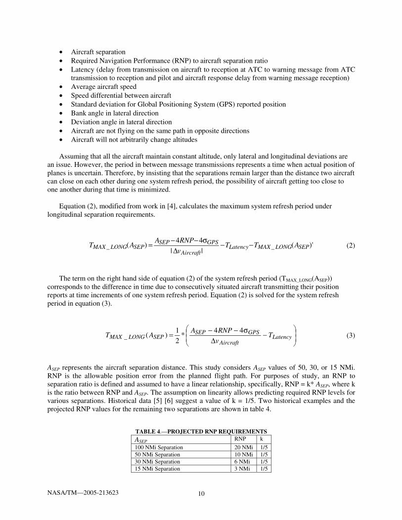
Equation (2), modified from work in [4], calculates the maximum system refresh period under longitudinal separation requirements.

)'(||

44)( __ SEPLONGMAXLatency

Aircraft

GPSSEPSEPLONGMAX ATT

v

RNPAAT −−

∆σ−−= (2)

The term on the right hand side of equation (2) of the system refresh period (TMAX_LONG(ASEP)) corresponds to the difference in time due to consecutively situated aircraft transmitting their position reports at time increments of one system refresh period. Equation (2) is solved for the system refresh period in equation (3).

⎟⎟

⎠

⎞

⎜⎜

⎝

⎛−

∆σ−−= Latency

Aircraft

GPSSEPSEPLONGMAX T

v

RNPAAT

44*

2

1)(_ (3)

ASEP represents the aircraft separation distance. This study considers ASEP values of 50, 30, or 15 NMi. RNP is the allowable position error from the planned flight path. For purposes of study, an RNP to separation ratio is defined and assumed to have a linear relationship, specifically, RNP = k* ASEP, where k is the ratio between RNP and ASEP. The assumption on linearity allows predicting required RNP levels for various separations. Historical data [5] [6] suggest a value of k = 1/5. Two historical examples and the projected RNP values for the remaining two separations are shown in table 4.

TABLE 4.—PROJECTED RNP REQUIREMENTS ASEP RNP k

100 NMi Separation 20 NMi 1/5 50 NMi Separation 10 NMi 1/5 30 NMi Separation 6 NMi 1/5 15 NMi Separation 3 NMi 1/5

NASA/TM—2005-213623 11

Other parameters in equation 3 are: • σGPS = 60 meter standard deviation for GPS

• hr

knotsvAircraft

/minutes60

10=∆ = relative aircraft to aircraft speed differential in NMi/min [7]

• TLatency = 7 minutes [7]

It should be noted that due to the value of the total latency, TLatency, it is possible for the maximum system refresh period to become a negative value. Since this is not allowed, the acceptable range for the maximum system refresh period is all real numbers greater than zero. Figure 12 plots the maximum system refresh period for the longitudinal separation component. Table 5 shows the maximum system refresh period for the three separations of interest.

Figure 12.—Maximum System Refresh Period–Longitudinal Separation.

TABLE 5.—MAXIMUM SYSTEM REFRESH PERIOD– LONGITUDINAL SEPARATION

Separation (NMi) Max. System Refresh Period (min)

50 NMi Separation 26.1



NASA/TM—2005-213623 12

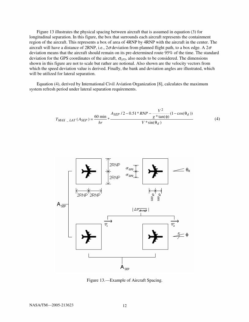
Figure 13 illustrates the physical spacing between aircraft that is assumed in equation (3) for longitudinal separation. In this figure, the box that surrounds each aircraft represents the containment region of the aircraft. This represents a box of area of 4RNP by 4RNP with the aircraft in the center. The aircraft will have a distance of 2RNP, i.e., 2σ deviation from planned flight path, to a box edge. A 2σ deviation means that the aircraft should remain on its pre-determined route 95% of the time. The standard deviation for the GPS coordinates of the aircraft, σGPS, also needs to be considered. The dimensions shown in this figure are not to scale but rather are notional. Also shown are the velocity vectors from which the speed deviation value is derived. Finally, the bank and deviation angles are illustrated, which will be utilized for lateral separation.

Equation (4), derived by International Civil Aviation Organization [8], calculates the maximum system refresh period under lateral separation requirements.

)sin(*

))cos(1()tan(*

*51.02/*

min60)(

2

_d

dSEP

SEPLATMAXV

g

VRNPA

hrAT

θ

θ−φ

−−= (4)

Figure 13.—Example of Aircraft Spacing.

NASA/TM—2005-213623 13

Parameters in equation 4 that are not previously defined are: • V = 540 knots average aircraft speed • g = 68584.32 NMi/hr2 acceleration due to gravity • φ= 15° Bank angle for aircraft relative to nadir • θd = 5.4° Deviation angle for aircraft relative to trajectory

Figure 14 plots the maximum system refresh period for the lateral separation component. Table 6

shows the maximum system refresh period for the three separations of interest.

Figure 14.—Maximum System Refresh Period–Lateral Separation.

TABLE 6.—MAXIMUM SYSTEM REFRESH PERIOD– LATERAL SEPARATION





Equation (5) shows the final equation used to compute the maximum system refresh period. It is the minimum of the maximum system refresh period for the longitudinal and lateral separations. ))(),(()( __ SEPLATMAXSEPLONGMAXSEPMAX ATATMINAT = (5)

NASA/TM—2005-213623 14

Figure 15 plots both the maximum system refresh period graphs together, with the longitudinal separation version in blue and the lateral separation version in red. Figure 16 plots the combined maximum system refresh period derived in equation (5). Table 7 shows the results for the three separations of interest.

Figure 15.—Maximum System Refresh Period–Longitudinal and Lateral Separations.

Figure 16.—Maximum System Refresh Period–Lateral/Longitudinal Separation.

NASA/TM—2005-213623 15

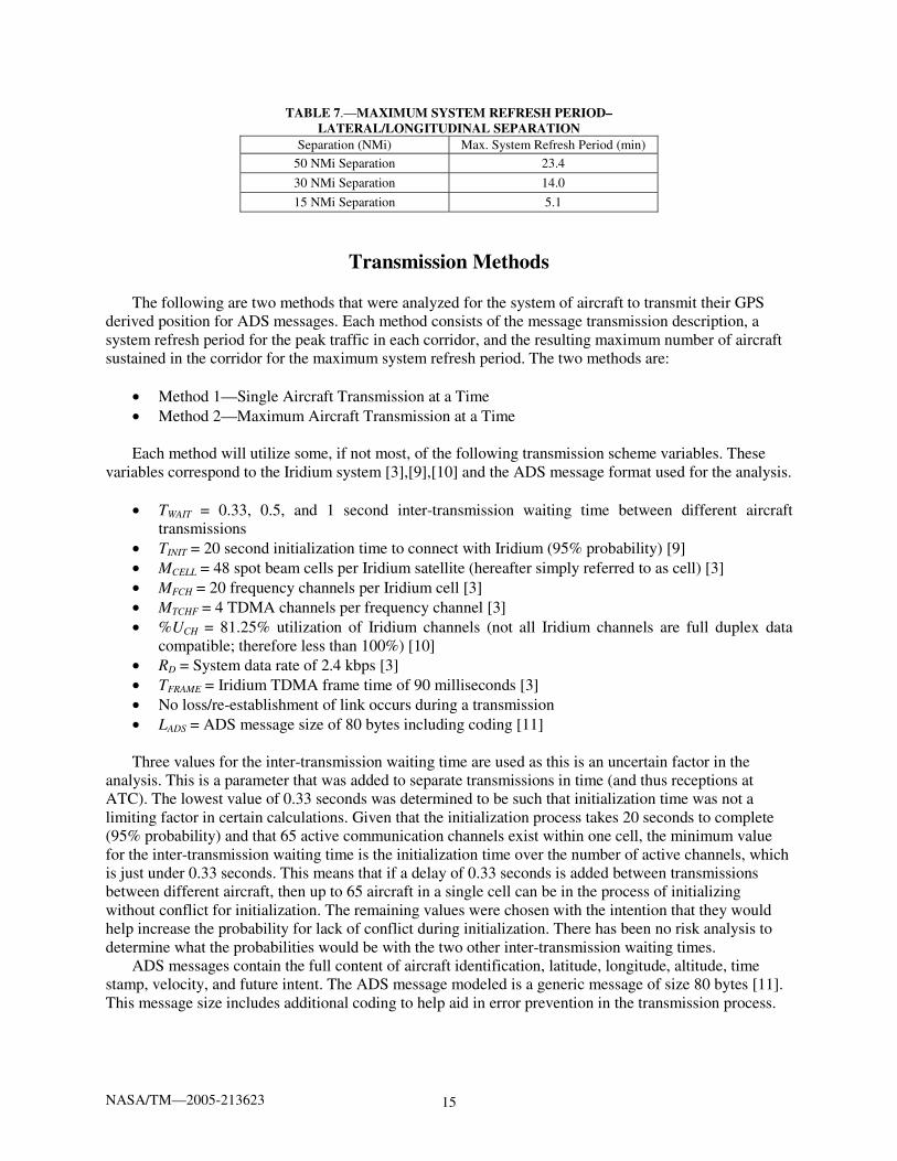
TABLE 7.—MAXIMUM SYSTEM REFRESH PERIOD– LATERAL/LONGITUDINAL SEPARATION





Transmission Methods

The following are two methods that were analyzed for the system of aircraft to transmit their GPS derived position for ADS messages. Each method consists of the message transmission description, a system refresh period for the peak traffic in each corridor, and the resulting maximum number of aircraft sustained in the corridor for the maximum system refresh period. The two methods are:

• Method 1—Single Aircraft Transmission at a Time • Method 2—Maximum Aircraft Transmission at a Time

Each method will utilize some, if not most, of the following transmission scheme variables. These

variables correspond to the Iridium system [3],[9],[10] and the ADS message format used for the analysis.

• TWAIT = 0.33, 0.5, and 1 second inter-transmission waiting time between different aircraft transmissions

• TINIT = 20 second initialization time to connect with Iridium (95% probability) [9] • MCELL = 48 spot beam cells per Iridium satellite (hereafter simply referred to as cell) [3] • MFCH = 20 frequency channels per Iridium cell [3] • MTCHF = 4 TDMA channels per frequency channel [3] • %UCH = 81.25% utilization of Iridium channels (not all Iridium channels are full duplex data

compatible; therefore less than 100%) [10] • RD = System data rate of 2.4 kbps [3] • TFRAME = Iridium TDMA frame time of 90 milliseconds [3] • No loss/re-establishment of link occurs during a transmission • LADS = ADS message size of 80 bytes including coding [11]

Three values for the inter-transmission waiting time are used as this is an uncertain factor in the

analysis. This is a parameter that was added to separate transmissions in time (and thus receptions at ATC). The lowest value of 0.33 seconds was determined to be such that initialization time was not a limiting factor in certain calculations. Given that the initialization process takes 20 seconds to complete (95% probability) and that 65 active communication channels exist within one cell, the minimum value for the inter-transmission waiting time is the initialization time over the number of active channels, which is just under 0.33 seconds. This means that if a delay of 0.33 seconds is added between transmissions between different aircraft, then up to 65 aircraft in a single cell can be in the process of initializing without conflict for initialization. The remaining values were chosen with the intention that they would help increase the probability for lack of conflict during initialization. There has been no risk analysis to determine what the probabilities would be with the two other inter-transmission waiting times.

ADS messages contain the full content of aircraft identification, latitude, longitude, altitude, time stamp, velocity, and future intent. The ADS message modeled is a generic message of size 80 bytes [11]. This message size includes additional coding to help aid in error prevention in the transmission process.

NASA/TM—2005-213623 16

Method 1

In the single aircraft transmission at a time method, two possibilities were considered. In the first case, the single transmitting aircraft is sending only its own position information. In the second case, the single transmitting aircraft is sending its own plus some of its neighbors’ position information.

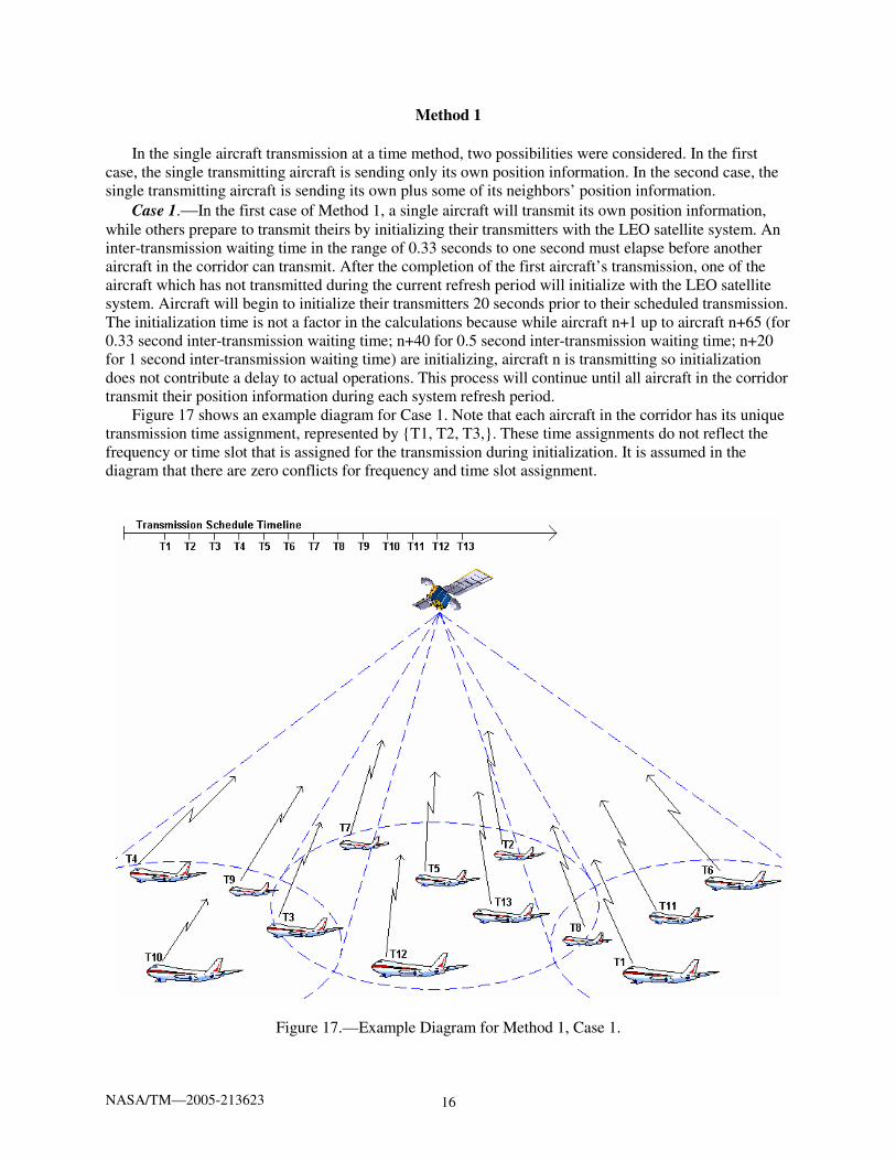
Case 1.—In the first case of Method 1, a single aircraft will transmit its own position information, while others prepare to transmit theirs by initializing their transmitters with the LEO satellite system. An inter-transmission waiting time in the range of 0.33 seconds to one second must elapse before another aircraft in the corridor can transmit. After the completion of the first aircraft’s transmission, one of the aircraft which has not transmitted during the current refresh period will initialize with the LEO satellite system. Aircraft will begin to initialize their transmitters 20 seconds prior to their scheduled transmission. The initialization time is not a factor in the calculations because while aircraft n+1 up to aircraft n+65 (for 0.33 second inter-transmission waiting time; n+40 for 0.5 second inter-transmission waiting time; n+20 for 1 second inter-transmission waiting time) are initializing, aircraft n is transmitting so initialization does not contribute a delay to actual operations. This process will continue until all aircraft in the corridor transmit their position information during each system refresh period.

Figure 17 shows an example diagram for Case 1. Note that each aircraft in the corridor has its unique transmission time assignment, represented by {T1, T2, T3,}. These time assignments do not reflect the frequency or time slot that is assigned for the transmission during initialization. It is assumed in the diagram that there are zero conflicts for frequency and time slot assignment.

Figure 17.—Example Diagram for Method 1, Case 1.

NASA/TM—2005-213623 17

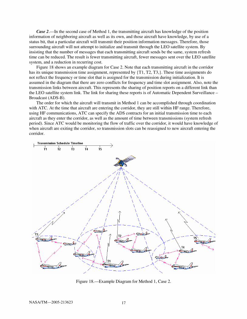
Case 2.—In the second case of Method 1, the transmitting aircraft has knowledge of the position information of neighboring aircraft as well as its own, and those aircraft have knowledge, by use of a status bit, that a particular aircraft will transmit their position information messages. Therefore, those surrounding aircraft will not attempt to initialize and transmit through the LEO satellite system. By insisting that the number of messages that each transmitting aircraft sends be the same, system refresh time can be reduced. The result is fewer transmitting aircraft, fewer messages sent over the LEO satellite system, and a reduction in recurring cost.

Figure 18 shows an example diagram for Case 2. Note that each transmitting aircraft in the corridor has its unique transmission time assignment, represented by {T1, T2, T3,}. These time assignments do not reflect the frequency or time slot that is assigned for the transmission during initialization. It is assumed in the diagram that there are zero conflicts for frequency and time slot assignment. Also, note the transmission links between aircraft. This represents the sharing of position reports on a different link than the LEO satellite system link. The link for sharing these reports is of Automatic Dependent Surveillance – Broadcast (ADS-B).

The order for which the aircraft will transmit in Method 1 can be accomplished through coordination with ATC. At the time that aircraft are entering the corridor, they are still within HF range. Therefore, using HF communications, ATC can specify the ADS contracts for an initial transmission time to each aircraft as they enter the corridor, as well as the amount of time between transmissions (system refresh period). Since ATC would be monitoring the flow of traffic over the corridor, it would have knowledge of when aircraft are exiting the corridor, so transmission slots can be reassigned to new aircraft entering the corridor.


NASA/TM—2005-213623 18

The required system refresh period for Method 1 is the minimum system refresh period that N number of aircraft will require to transmit their position information to ATC once. This minimum system refresh period, (TMIN1(N,b)), is a function of the number of aircraft in the corridor (N) and the number of messages per transmission (b). Equation (6) computes the minimum system refresh period.

⎟⎟⎠

⎞⎜⎜⎝

⎛⎥⎥

⎤⎢⎢

⎡∗

⎟⎟⎟⎟⎟

⎠

⎞

⎜⎜⎜⎜⎜

⎝

⎛+⎥

⎥

⎤⎢⎢

⎡

∗∗∗

=b

NT

TR

LbT

bNTWAIT

FRAMED

ADSFRAME

MINminsec/60

*8

),(1 (6)

where:

• N = number of aircraft in the corridor • b = number of messages per transmission • LADS = length of ADS message of 80 bytes • TFRAME = Iridium TDMA frame time of 0.090 seconds • RD = System data rate of 2.4 kbps • TWAIT = 0.33, 0.5, and 1 second inter-transmission waiting times between different aircraft

transmissions

Tables 8 through 10 show the minimum system refresh period for the peak traffic load of 108 aircraft for the Northern Pacific Corridor (23 aircraft for the Western Hawaiian Corridor and 46 aircraft for the Eastern Hawaiian Corridor) over the three inter-transmission waiting times. Note that one message per transmission is the first case (b = 1); a single aircraft transmitting its own position information. Two or more messages per transmission are the second case (b > 1) where one aircraft is transmitting position information for itself plus as many as 11 other aircraft in its ADS vicinity.

TABLE 8.—REQUIRED SYSTEM REFRESH PERIOD (MINUTES) 0— NORTHERN PACIFIC CORRIDOR

Messages per Transmission Inter-Transmission Waiting Time 0.33 sec 0.5 sec 1.0 sec

1 1.08 1.39 2.29 2 0.78 0.94 1.39 4 0.63 0.71 0.94

12 0.54 0.56 0.64

TABLE 9.—REQUIRED SYSTEM REFRESH PERIOD (MINUTES)– WESTERN HAWAIIAN CORRIDOR


1 0.23 0.30 0.49 2 0.17 0.21 0.31 4 0.14 0.16 0.21

12 0.12 0.12 0.14

TABLE 10.—REQUIRED SYSTEM REFRESH PERIOD (MINUTES)– EASTERN HAWAIIAN CORRIDOR


1 0.46 0.59 0.97 2 0.33 0.40 0.59 4 0.28 0.32 0.42

12 0.24 0.25 0.28

NASA/TM—2005-213623 19

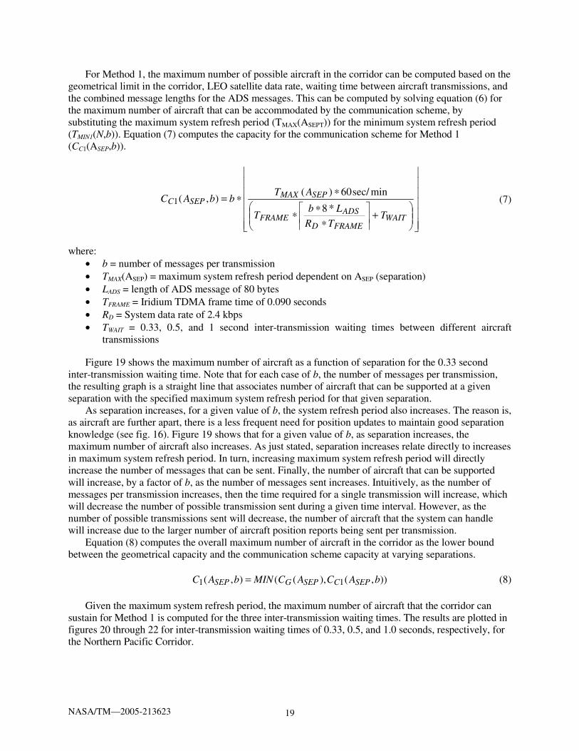
For Method 1, the maximum number of possible aircraft in the corridor can be computed based on the geometrical limit in the corridor, LEO satellite data rate, waiting time between aircraft transmissions, and the combined message lengths for the ADS messages. This can be computed by solving equation (6) for the maximum number of aircraft that can be accommodated by the communication scheme, by substituting the maximum system refresh period (TMAX(ASEPT)) for the minimum system refresh period (TMIN1(N,b)). Equation (7) computes the capacity for the communication scheme for Method 1 (CC1(ASEP,b)).

⎥⎥⎥⎥⎥

⎦

⎥

⎢⎢⎢⎢⎢

⎣

⎢

⎟⎟⎠

⎞⎜⎜⎝

⎛+⎥

⎥

⎤⎢⎢

⎡

∗∗∗

∗∗=

WAITFRAMED

ADSFRAME

SEPMAXSEPC

TTR

LbT

ATbbAC

*8

minsec/60)(),(1 (7)

where:

• b = number of messages per transmission • TMAX(ASEP) = maximum system refresh period dependent on ASEP (separation) • LADS = length of ADS message of 80 bytes • TFRAME = Iridium TDMA frame time of 0.090 seconds • RD = System data rate of 2.4 kbps • TWAIT = 0.33, 0.5, and 1 second inter-transmission waiting times between different aircraft

transmissions

Figure 19 shows the maximum number of aircraft as a function of separation for the 0.33 second inter-transmission waiting time. Note that for each case of b, the number of messages per transmission, the resulting graph is a straight line that associates number of aircraft that can be supported at a given separation with the specified maximum system refresh period for that given separation.

As separation increases, for a given value of b, the system refresh period also increases. The reason is, as aircraft are further apart, there is a less frequent need for position updates to maintain good separation knowledge (see fig. 16). Figure 19 shows that for a given value of b, as separation increases, the maximum number of aircraft also increases. As just stated, separation increases relate directly to increases in maximum system refresh period. In turn, increasing maximum system refresh period will directly increase the number of messages that can be sent. Finally, the number of aircraft that can be supported will increase, by a factor of b, as the number of messages sent increases. Intuitively, as the number of messages per transmission increases, then the time required for a single transmission will increase, which will decrease the number of possible transmission sent during a given time interval. However, as the number of possible transmissions sent will decrease, the number of aircraft that the system can handle will increase due to the larger number of aircraft position reports being sent per transmission.

Equation (8) computes the overall maximum number of aircraft in the corridor as the lower bound between the geometrical capacity and the communication scheme capacity at varying separations. )),(),((),( 11 bACACMINbAC SEPCSEPGSEP = (8)

Given the maximum system refresh period, the maximum number of aircraft that the corridor can sustain for Method 1 is computed for the three inter-transmission waiting times. The results are plotted in figures 20 through 22 for inter-transmission waiting times of 0.33, 0.5, and 1.0 seconds, respectively, for the Northern Pacific Corridor.

NASA/TM—2005-213623 20

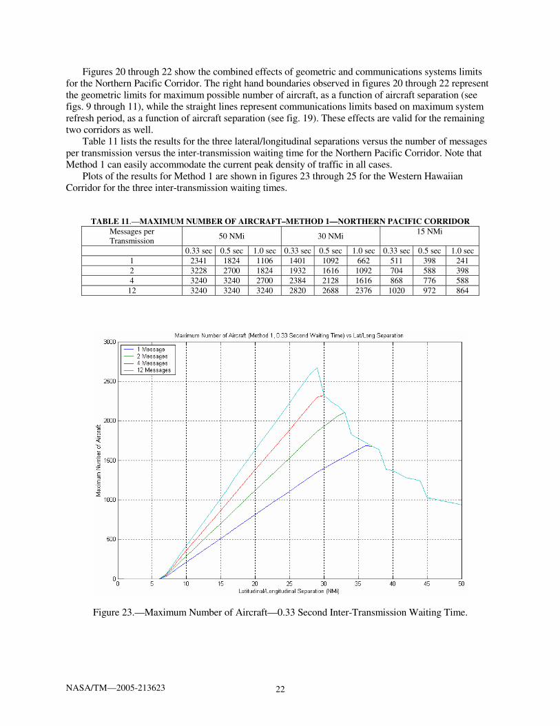
Figure 19.—Maximum Number of Aircraft—0.33 Second Inter-Transmission Waiting Time.


NASA/TM—2005-213623 21



NASA/TM—2005-213623 22

Figures 20 through 22 show the combined effects of geometric and communications systems limits for the Northern Pacific Corridor. The right hand boundaries observed in figures 20 through 22 represent the geometric limits for maximum possible number of aircraft, as a function of aircraft separation (see figs. 9 through 11), while the straight lines represent communications limits based on maximum system refresh period, as a function of aircraft separation (see fig. 19). These effects are valid for the remaining two corridors as well.

Table 11 lists the results for the three lateral/longitudinal separations versus the number of messages per transmission versus the inter-transmission waiting time for the Northern Pacific Corridor. Note that Method 1 can easily accommodate the current peak density of traffic in all cases.

Plots of the results for Method 1 are shown in figures 23 through 25 for the Western Hawaiian Corridor for the three inter-transmission waiting times.

TABLE 11.—MAXIMUM NUMBER OF AIRCRAFT–METHOD 1—NORTHERN PACIFIC CORRIDOR Messages per Transmission

50 NMi 30 NMi 15 NMi

0.33 sec 0.5 sec 1.0 sec 0.33 sec 0.5 sec 1.0 sec 0.33 sec 0.5 sec 1.0 sec 1 2341 1824 1106 1401 1092 662 511 398 241 2 3228 2700 1824 1932 1616 1092 704 588 398 4 3240 3240 2700 2384 2128 1616 868 776 588

12 3240 3240 3240 2820 2688 2376 1020 972 864


NASA/TM—2005-213623 23



NASA/TM—2005-213623 24

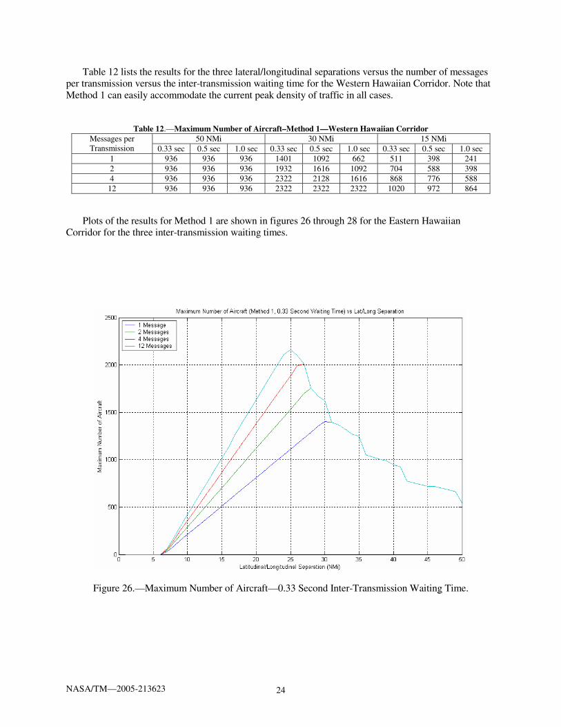
Table 12 lists the results for the three lateral/longitudinal separations versus the number of messages per transmission versus the inter-transmission waiting time for the Western Hawaiian Corridor. Note that Method 1 can easily accommodate the current peak density of traffic in all cases.

Table 12.—Maximum Number of Aircraft–Method 1—Western Hawaiian Corridor 50 NMi 30 NMi 15 NMi Messages per

Transmission 0.33 sec 0.5 sec 1.0 sec 0.33 sec 0.5 sec 1.0 sec 0.33 sec 0.5 sec 1.0 sec 1 936 936 936 1401 1092 662 511 398 241 2 936 936 936 1932 1616 1092 704 588 398 4 936 936 936 2322 2128 1616 868 776 588

12 936 936 936 2322 2322 2322 1020 972 864

Plots of the results for Method 1 are shown in figures 26 through 28 for the Eastern Hawaiian Corridor for the three inter-transmission waiting times.


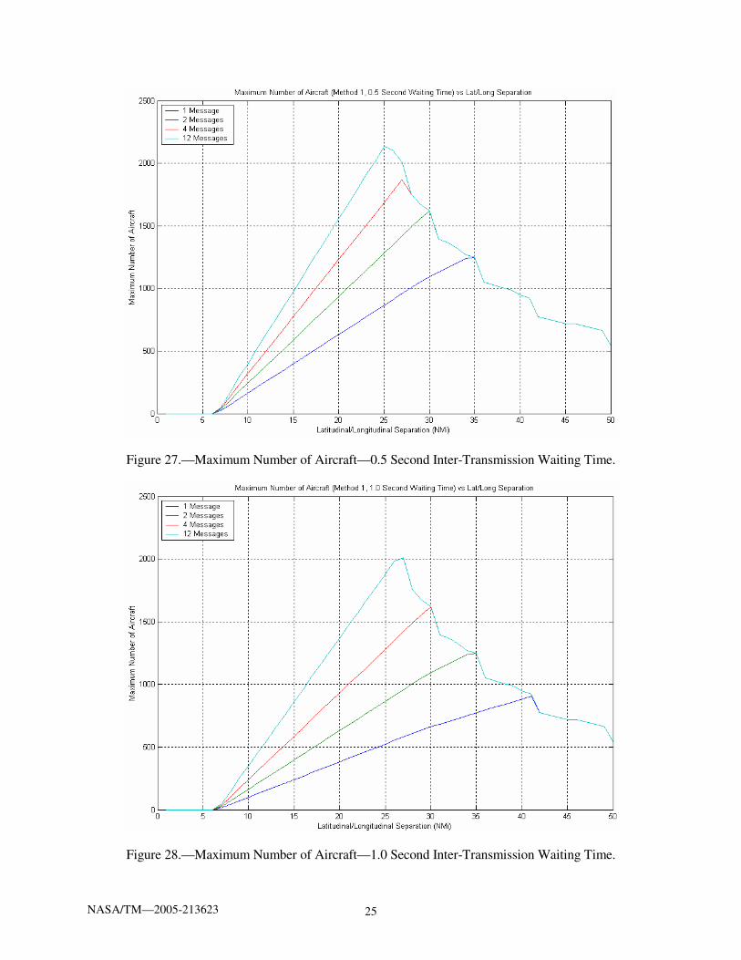
NASA/TM—2005-213623 25



NASA/TM—2005-213623 26

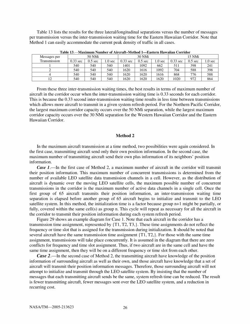
Table 13 lists the results for the three lateral/longitudinal separations versus the number of messages per transmission versus the inter-transmission waiting time for the Eastern Hawaiian Corridor. Note that Method 1 can easily accommodate the current peak density of traffic in all cases.

Table 13.—Maximum Number of Aircraft–Method 1—Eastern Hawaiian Corridor

50 NMi 30 NMi 15 NMi Messages per Transmission 0.33 sec 0.5 sec 1.0 sec 0.33 sec 0.5 sec 1.0 sec 0.33 sec 0.5 sec 1.0 sec

1 540 540 540 1401 1092 662 511 398 241 2 540 540 540 1620 1616 1092 704 588 398 4 540 540 540 1620 1620 1616 868 776 588

12 540 540 540 1620 1620 1620 1020 972 864

From these three inter-transmission waiting times, the best results in terms of maximum number of aircraft in the corridor occur when the inter-transmission waiting time is 0.33 seconds for each corridor. This is because the 0.33 second inter-transmission waiting time results in less time between transmissions which allows more aircraft to transmit in a given system refresh period. For the Northern Pacific Corridor, the largest maximum corridor capacity occurs over the 50 NMi separation, while the largest maximum corridor capacity occurs over the 30 NMi separation for the Western Hawaiian Corridor and the Eastern Hawaiian Corridor.

Method 2

In the maximum aircraft transmission at a time method, two possibilities were again considered. In the first case, transmitting aircraft send only their own position information. In the second case, the maximum number of transmitting aircraft send their own plus information of its neighbors’ position information.

Case 1.—In the first case of Method 2, a maximum number of aircraft in the corridor will transmit their position information. This maximum number of concurrent transmissions is determined from the number of available LEO satellite data transmission channels in a cell. However, as the distribution of aircraft is dynamic over the moving LEO satellite cells, the maximum possible number of concurrent transmissions in the corridor is the maximum number of active data channels in a single cell. Once the first group of 65 aircraft transmits their position information, an inter-transmission waiting time separation is elapsed before another group of 65 aircraft begins to initialize and transmit to the LEO satellite system. In this method, the initialization time is a factor because group n+1 might be partially, or fully, covered within the same cell(s) as group n. This cycle will repeat as necessary for all the aircraft in the corridor to transmit their position information during each system refresh period.

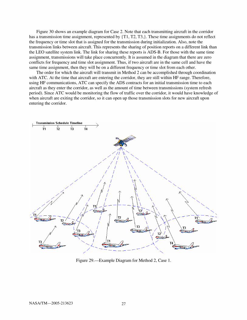
Figure 29 shows an example diagram for Case 1. Note that each aircraft in the corridor has a transmission time assignment, represented by {T1, T2, T3,}. These time assignments do not reflect the frequency or time slot that is assigned for the transmission during initialization. It should be noted that several aircraft have the same transmission time assignment {T1, T2,}. For those with the same time assignment, transmissions will take place concurrently. It is assumed in the diagram that there are zero conflicts for frequency and time slot assignment. Thus, if two aircraft are in the same cell and have the same time assignment, then they will be on a different frequency or time slot from each other.

Case 2.—In the second case of Method 2, the transmitting aircraft have knowledge of the position information of surrounding aircraft as well as their own, and those aircraft have knowledge that a set of aircraft will transmit their position information messages. Therefore, those surrounding aircraft will not attempt to initialize and transmit through the LEO satellite system. By insisting that the number of messages that each transmitting aircraft sends be the same, system refresh time can be reduced. The result is fewer transmitting aircraft, fewer messages sent over the LEO satellite system, and a reduction in recurring cost.

NASA/TM—2005-213623 27

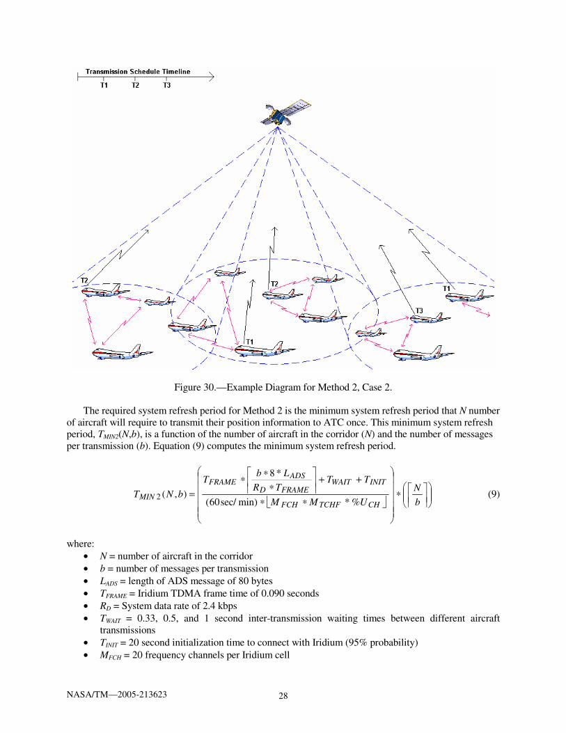
Figure 30 shows an example diagram for Case 2. Note that each transmitting aircraft in the corridor has a transmission time assignment, represented by {T1, T2, T3,}. These time assignments do not reflect the frequency or time slot that is assigned for the transmission during initialization. Also, note the transmission links between aircraft. This represents the sharing of position reports on a different link than the LEO satellite system link. The link for sharing these reports is ADS-B. For those with the same time assignment, transmissions will take place concurrently. It is assumed in the diagram that there are zero conflicts for frequency and time slot assignment. Thus, if two aircraft are in the same cell and have the same time assignment, then they will be on a different frequency or time slot from each other.

The order for which the aircraft will transmit in Method 2 can be accomplished through coordination with ATC. At the time that aircraft are entering the corridor, they are still within HF range. Therefore, using HF communications, ATC can specify the ADS contracts for an initial transmission time to each aircraft as they enter the corridor, as well as the amount of time between transmissions (system refresh period). Since ATC would be monitoring the flow of traffic over the corridor, it would have knowledge of when aircraft are exiting the corridor, so it can open up those transmission slots for new aircraft upon entering the corridor.


NASA/TM—2005-213623 28


The required system refresh period for Method 2 is the minimum system refresh period that N number of aircraft will require to transmit their position information to ATC once. This minimum system refresh period, TMIN2(N,b), is a function of the number of aircraft in the corridor (N) and the number of messages per transmission (b). Equation (9) computes the minimum system refresh period.

⎣ ⎦

⎟⎟⎠

⎞⎜⎜⎝

⎛⎥⎥

⎤⎢⎢

⎡∗

⎟⎟⎟⎟⎟

⎠

⎞

⎜⎜⎜⎜⎜

⎝

⎛

∗∗

++⎥⎥

⎤⎢⎢

⎡

∗∗∗

=b

N

UMM

TTTR

LbT

bNTCHTCHFFCH

INITWAITFRAMED

ADSFRAME

MIN%*min)sec/60(

*8

),(2 (9)

where:

• N = number of aircraft in the corridor • b = number of messages per transmission • LADS = length of ADS message of 80 bytes • TFRAME = Iridium TDMA frame time of 0.090 seconds • RD = System data rate of 2.4 kbps • TWAIT = 0.33, 0.5, and 1 second inter-transmission waiting times between different aircraft

transmissions • TINIT = 20 second initialization time to connect with Iridium (95% probability) • MFCH = 20 frequency channels per Iridium cell

NASA/TM—2005-213623 29

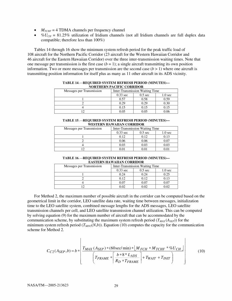
• MTCHF = 4 TDMA channels per frequency channel • %UCH = 81.25% utilization of Iridium channels (not all Iridium channels are full duplex data

compatible; therefore less than 100%)

Tables 14 through 16 show the minimum system refresh period for the peak traffic load of 108 aircraft for the Northern Pacific Corridor (23 aircraft for the Western Hawaiian Corridor and 46 aircraft for the Eastern Hawaiian Corridor) over the three inter-transmission waiting times. Note that one message per transmission is the first case (b = 1); a single aircraft transmitting its own position information. Two or more messages per transmission are the second case (b > 1) where one aircraft is transmitting position information for itself plus as many as 11 other aircraft in its ADS vicinity.

TABLE 14.—REQUIRED SYSTEM REFRESH PERIOD (MINUTES)— NORTHERN PACIFIC CORRIDOR

Inter-Transmission Waiting Time Messages per Transmission 0.33 sec 0.5 sec 1.0 sec

1 0.57 0.58 0.59 2 0.29 0.29 0.30 4 0.15 0.15 0.15

12 0.05 0.05 0.06

TABLE 15.—REQUIRED SYSTEM REFRESH PERIOD (MINUTES)—

WESTERN HAWAIIAN CORRIDOR Inter-Transmission Waiting Time Messages per Transmission

0.33 sec 0.5 sec 1.0 sec 1 0.12 0.12 0.13 2 0.06 0.06 0.07 4 0.03 0.03 0.03

12 0.01 0.01 0.01

TABLE 16.—REQUIRED SYSTEM REFRESH PERIOD (MINUTES)— EASTERN HAWAIIAN CORRIDOR

Inter-Transmission Waiting Time Messages per Transmission 0.33 sec 0.5 sec 1.0 sec

1 0.24 0.24 0.25 2 0.12 0.12 0.13 4 0.07 0.07 0.07

12 0.02 0.02 0.02

For Method 2, the maximum number of possible aircraft in the corridor can be computed based on the

geometrical limit in the corridor, LEO satellite data rate, waiting time between messages, initialization time to the LEO satellite system, combined message lengths for the ADS messages, LEO satellite transmission channels per cell, and LEO satellite transmission channel utilization. This can be computed by solving equation (9) for the maximum number of aircraft that can be accommodated by the communication scheme, by substituting the maximum system refresh period (TMAX (ASEP)) for the minimum system refresh period (TMIN2(N,b)). Equation (10) computes the capacity for the communication scheme for Method 2.

⎣ ⎦

⎥⎥⎥⎥⎥

⎦

⎥

⎢⎢⎢⎢⎢

⎣

⎢

⎟⎟⎠

⎞⎜⎜⎝

⎛++⎥

⎥

⎤⎢⎢

⎡

∗∗∗

∗∗∗∗=

INITWAITFRAMED

ADSFRAME

CHTCHFFCHSEPMAXSEPC

TTTR

LbT

UMMATbbAC

*8

%*min)sec/60()(),(2 (10)

NASA/TM—2005-213623 30

where:

• b = number of messages per transmission • TMAX(ASEP) = maximum system refresh period dependent on ASEP (separation) • LADS = length of ADS message of 80 bytes • TFRAME = Iridium TDMA frame time of 0.090 seconds • RD = System data rate of 2.4 kbps • TWAIT = 0.33, 0.5, and 1 second inter-transmission waiting times between different aircraft

transmissions • TINIT = 20 second initialization time to connect with Iridium (95% probability) • MFCH = 20 frequency channels per Iridium cell • MTCHF = 4 TDMA channels per frequency channel • %UCH = 81.25% utilization of Iridium channels (not all Iridium channels are full duplex data

compatible; therefore less than 100%)

Equation (11) computes the overall maximum number of aircraft in the corridor as the lower bound between the geometrical capacity and the communication scheme capacity at varying separations. )),(),((),( 22 bACACMINbAC SEPCSEPGSEP = (11)

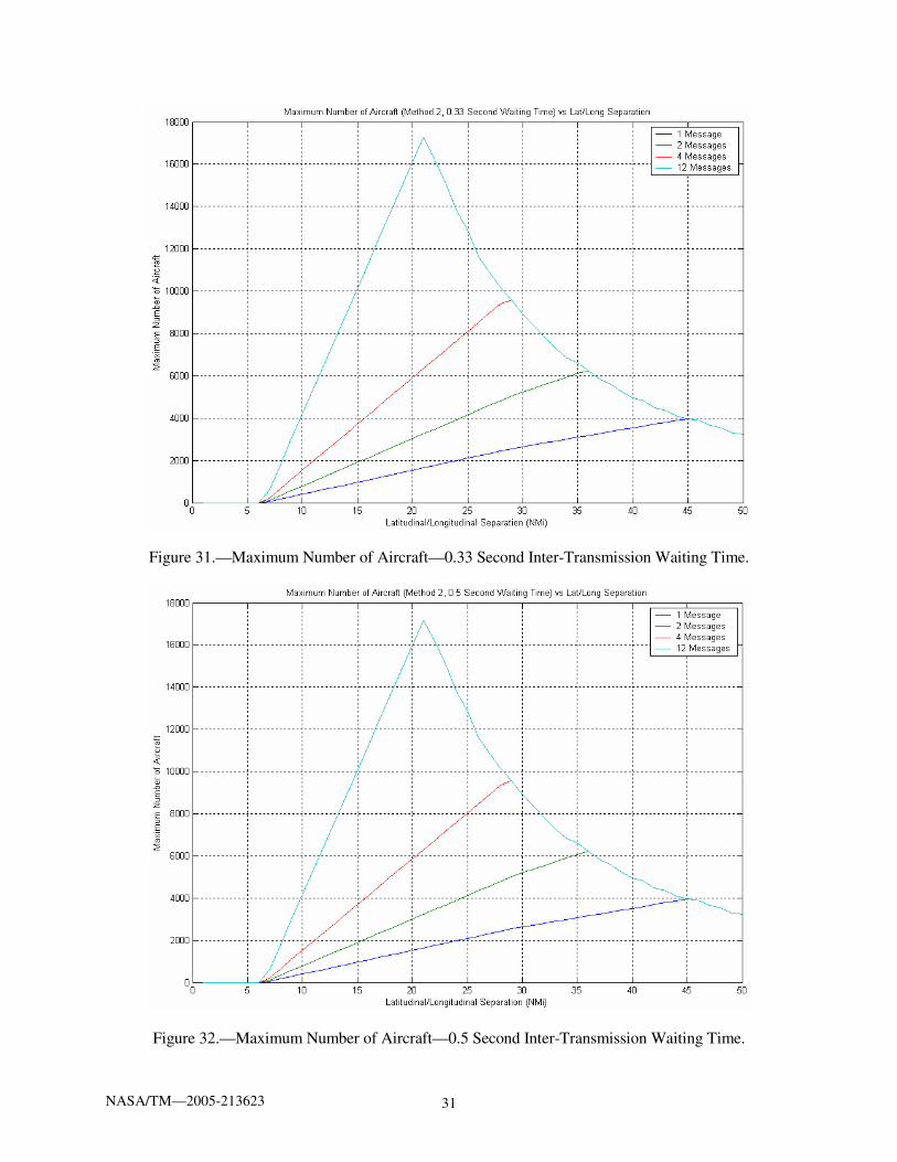
Given the maximum system refresh period, the maximum number of aircraft that the corridor can sustain for Method 2 is computed for the three inter-transmission waiting times. The results are plotted in figures 31 through 33 for inter-transmission waiting times of 0.33, 0.5, and 1.0 seconds, respectively, for the Northern Pacific Corridor.

Figures 31 through 33 show the combined effects of geometric and communications systems limits for the Northern Pacific Corridor. The right hand boundaries observed in figures 31 through 33 represent the geometric limits for maximum possible number of aircraft, as a function of aircraft separation (see figs. 9 through 11), while the straight lines represent communications limits based on maximum system refresh period, as a function of aircraft separation (see fig. 19). These effects are valid for the remaining two corridors as well.

Table 17 lists the results for the three lateral/longitudinal separations versus the number of messages per transmission versus the inter-transmission waiting time for the Northern Pacific Corridor. Note that Method 2 can easily accommodate the current peak density of traffic in all cases.

TABLE 17.—MAXIMUM NUMBER OF AIRCRAFT–METHOD 2—NORTHERN PACIFIC CORRIDOR 50 NMi 30 NMi 15 NMi Messages per


12 3240 3240 3240 8910 8910 8910 10140 10068 9864

NASA/TM—2005-213623 31



NASA/TM—2005-213623 32

Figure 33.—Maximum Number of Aircraft—1.0 Second Inter-Transmission Waiting Time


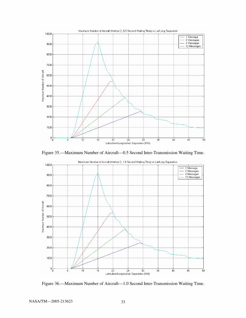
Plots of the results for Method 2 are shown in figures 34 through 36 for the Western Hawaiian Corridor for the three inter-transmission waiting times.

NASA/TM—2005-213623 33



NASA/TM—2005-213623 34

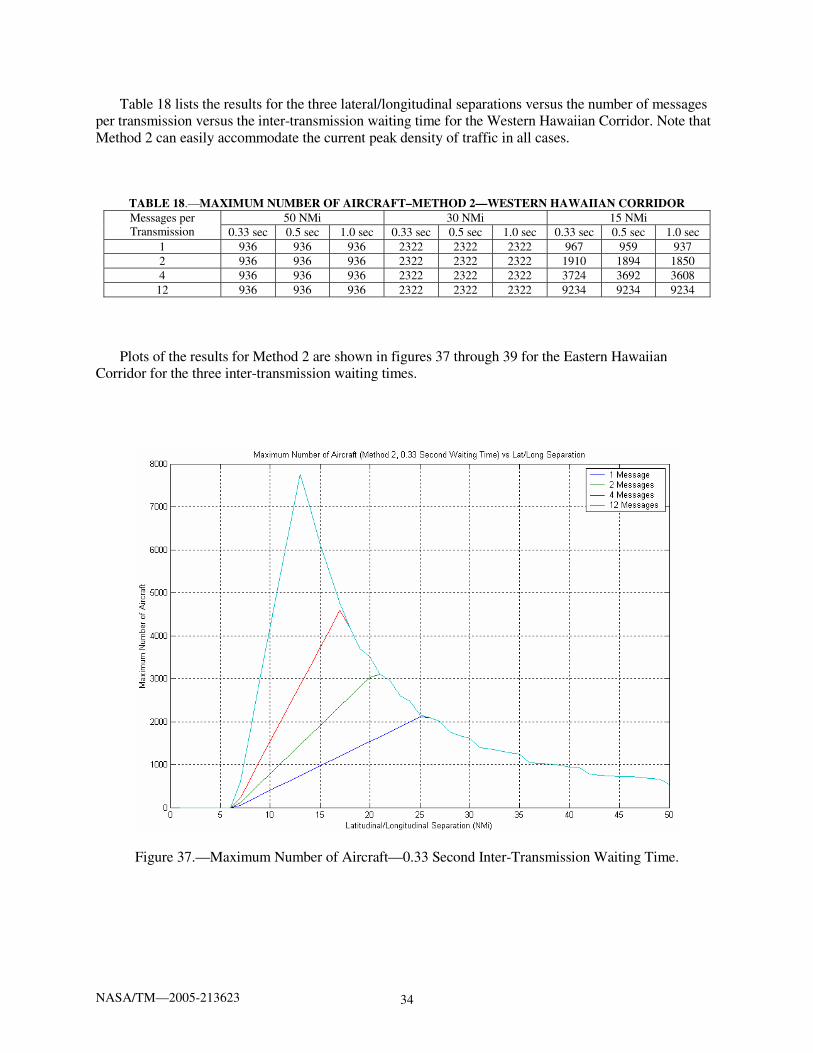
Table 18 lists the results for the three lateral/longitudinal separations versus the number of messages per transmission versus the inter-transmission waiting time for the Western Hawaiian Corridor. Note that Method 2 can easily accommodate the current peak density of traffic in all cases.

TABLE 18.—MAXIMUM NUMBER OF AIRCRAFT–METHOD 2—WESTERN HAWAIIAN CORRIDOR 50 NMi 30 NMi 15 NMi Messages per


12 936 936 936 2322 2322 2322 9234 9234 9234

Plots of the results for Method 2 are shown in figures 37 through 39 for the Eastern Hawaiian Corridor for the three inter-transmission waiting times.


NASA/TM—2005-213623 35



NASA/TM—2005-213623 36

Table 19 lists the results for the three lateral/longitudinal separations versus the number of messages per transmission versus the inter-transmission waiting time for the Eastern Hawaiian Corridor. Note that Method 2 can easily accommodate the current peak density of traffic in all cases.

TABLE 19.—MAXIMUM NUMBER OF AIRCRAFT–METHOD 2—EASTERN HAWAIIAN CORRIDOR Messages per Transmission

50 NMi 30 NMi 15 NMi

0.33 sec 0.5 sec 1.0 sec 0.33 sec 0.5 sec 1.0 sec 0.33 sec 0.5 sec 1.0 sec 1 540 540 540 1620 1620 1620 967 959 937 2 540 540 540 1620 1620 1620 1910 1894 1850 4 540 540 540 1620 1620 1620 3724 3692 3608

12 540 540 540 1620 1620 1620 6120 6120 6120

From these three inter-transmission waiting times, the best results in terms of maximum number of aircraft in the corridor occur when the inter-transmission waiting time is 0.33 seconds for each corridor. This is because the 0.33 second inter-transmission waiting time results in less time between transmissions which allows more aircraft to transmit in a given system refresh period. For all three corridors, the largest maximum corridor capacity occurs over the 15 NMi separation.

Corridor Loading Improvement

Having shown two methods for which the system of aircraft can transmit their data to ATC within the maximum allowed system refresh period, a traffic loading improvement measure will be considered.

The measure compares the maximum number of aircraft of the two transmission methods against the current peak traffic density of each corridor. A single message per transmission (b = 1) represents an aircraft having to know only its own position, which is the worst case scenario for the system. Table 20 shows the percent differences between the 267 aircraft of the Northern Pacific Corridor and the number of aircraft calculated previously and shown in table 11 (for Method 1) and table 17 (for Method 2). Tables 21 and 22 show the percent differences for the Western Hawaiian Corridor (23 aircraft peak traffic density) and the Eastern Hawaiian Corridor (46 aircraft peak traffic density), referencing tables 12 and 13 (for Method 1) and 18 and 19 (for Method 2), respectively. Tables 20 through 22 are based on equation (12), where N represents the number of aircraft that can be placed in the corridor at the specified separations for any of the three inter-transmission waiting times. NCP is the current peak traffic density for each corridor.

CP

CP

N

NNIncrease

−= *100% (12)

Tables 20 through 22 show the largest overall percentage increase in traffic over the current peak traffic density in each corridor occurs with the following conditions:

15 NMi separation Method 2 12 messages per transmission Any of the three inter-transmission waiting times (Northern Pacific Corridor is exception with

maximum occurring with a 0.33 second inter-transmission waiting time)

If implementation allows only a single message per transmission, then the largest percentage increase in traffic density occurs with the following conditions:

30 NMi separation (Western Hawaiian Corridor and Eastern Hawaiian Corridor) 50 NMi separation (Northern Pacific Corridor) Method 2 Any of the three inter-transmission waiting times

NASA/TM—2005-213623 37

TABLE 20.—ABSOLUTE PERCENT INCREASE IN MAXIMUM AIRCRAFT– NORTHERN PACIFIC CORRIDOR

Method 1 Method 2 Lat/Long Separation

b 0.33 sec

0.5 sec

1.0 sec

0.33 sec

0.5 sec

1.0 sec

1 2068 1589 924 2900 2900 2900

2 2889 2400 1589 2900 2900 2900

4 2900 2900 2900 2900 2900 2900 50 NMi Separation

12 2900 2900 2900 2900 2900 2900

1 1197 911 513 2356 2336 2279

2 1689 1396 911 4748 4709 4598

4 2107 1870 1396 8150 8150 8150 30 NMi Separation

12 2511 2389 2100 8150 8150 8150

1 373 269 123 795 788 768

2 552 444 269 1669 1654 1613

4 704 619 444 3348 3319 3241 15 NMi Separation

12 844 800 700 9289 9222 9033

TABLE 21.—ABSOLUTE PERCENT INCREASE IN MAXIMUM AIRCRAFT– WESTERN HAWAIIAN CORRIDOR

Method 1 Method 2 Lat/Long Separation

b 0.33 sec

0.5 sec

1.0 sec

0.33 sec

0.5 sec

1.0 sec

1 3970 3970 3970 3970 3970 3970

2 3970 3970 3970 3970 3970 3970

4 3970 3970 3970 3970 3970 3970 50 NMi Separation

12 3970 3970 3970 3970 3970 3970

1 5991 4648 2778 9996 9996 9996

2 8300 6926 4648 9996 9996 9996

4 9996 9152 6926 9996 9996 9996 30 NMi Separation

12 9996 9996 9996 9996 9996 9996

1 2122 1630 948 4104 4070 3974

2 2961 2457 1630 8204 8135 7943

4 3674 3274 2457 16091 15952 15587 15 NMi Separation

12 4335 4126 3657 40048 40048 40048

NASA/TM—2005-213623 38

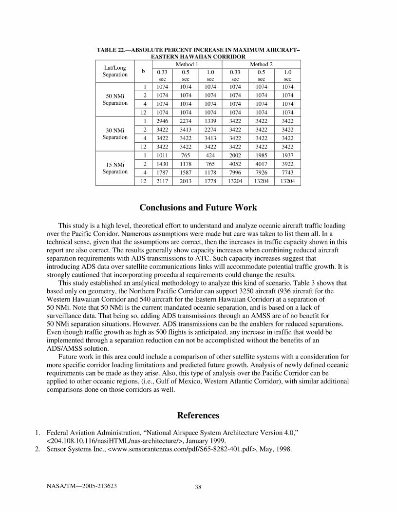
TABLE 22.—ABSOLUTE PERCENT INCREASE IN MAXIMUM AIRCRAFT– EASTERN HAWAIIAN CORRIDOR

Method 1 Method 2 Lat/Long

Separation b 0.33

sec 0.5 sec

1.0 sec

0.33 sec

0.5 sec

1.0 sec

1 1074 1074 1074 1074 1074 1074

2 1074 1074 1074 1074 1074 1074

4 1074 1074 1074 1074 1074 1074 50 NMi

Separation

12 1074 1074 1074 1074 1074 1074

1 2946 2274 1339 3422 3422 3422

2 3422 3413 2274 3422 3422 3422

4 3422 3422 3413 3422 3422 3422 30 NMi

Separation

12 3422 3422 3422 3422 3422 3422

1 1011 765 424 2002 1985 1937

2 1430 1178 765 4052 4017 3922

4 1787 1587 1178 7996 7926 7743 15 NMi

Separation

12 2117 2013 1778 13204 13204 13204

Conclusions and Future Work

This study is a high level, theoretical effort to understand and analyze oceanic aircraft traffic loading over the Pacific Corridor. Numerous assumptions were made but care was taken to list them all. In a technical sense, given that the assumptions are correct, then the increases in traffic capacity shown in this report are also correct. The results generally show capacity increases when combining reduced aircraft separation requirements with ADS transmissions to ATC. Such capacity increases suggest that introducing ADS data over satellite communications links will accommodate potential traffic growth. It is strongly cautioned that incorporating procedural requirements could change the results.

This study established an analytical methodology to analyze this kind of scenario. Table 3 shows that based only on geometry, the Northern Pacific Corridor can support 3250 aircraft (936 aircraft for the Western Hawaiian Corridor and 540 aircraft for the Eastern Hawaiian Corridor) at a separation of 50 NMi. Note that 50 NMi is the current mandated oceanic separation, and is based on a lack of surveillance data. That being so, adding ADS transmissions through an AMSS are of no benefit for 50 NMi separation situations. However, ADS transmissions can be the enablers for reduced separations. Even though traffic growth as high as 500 flights is anticipated, any increase in traffic that would be implemented through a separation reduction can not be accomplished without the benefits of an ADS/AMSS solution.

Future work in this area could include a comparison of other satellite systems with a consideration for more specific corridor loading limitations and predicted future growth. Analysis of newly defined oceanic requirements can be made as they arise. Also, this type of analysis over the Pacific Corridor can be applied to other oceanic regions, (i.e., Gulf of Mexico, Western Atlantic Corridor), with similar additional comparisons done on those corridors as well.

References

1. Federal Aviation Administration, “National Airspace System Architecture Version 4.0,” <204.108.10.116/nasiHTML/nas-architecture/>, January 1999.

2. Sensor Systems Inc., <www.sensorantennas.com/pdf/S65-8282-401.pdf>, May, 1998.

NASA/TM—2005-213623 39

3. Fossa, Carl E., Raines, Richard A., Gunsch, Gregg H., Temple, Michael A., “An Overview of the Iridium Low Earth Orbit (LEO) Satellite System,” IEEE, 1998.

4. Flax, Bennett, “A Minimum Rate of Position Reporting in the Future Oceanic Air Traffic Control System,” IEEE Plans `92, March 1992.

5. Shakarian, Arek, Haraldsdottir, Aslaug, “Required Total System Performance and Results of a Short Term Conflict Alert Simulation Study,” 4th US/Europe Air Traffic Management R & D Seminar, Sante Fe, December 2001.

6. Aimer, Jeff, “Required Navigation Performance for Improved Flight Operations and Efficient Use of Airspace,” <www.boeing.com/commercial/aeromagazine/aero_12/navigation.pdf>, October 2000.

7. Morse, David, Griep, Karl, “Next Generation FANS Over Inmarsat Broadband Global Area Network (BGAN),” 23rd DASC Conference, Salt Lake City, Utah, October 24–28, 2004.

8. ICAO Document 9689, “Manual on Airspace Planning Methodology for the Determination of Separation Minima,” First Edition, 1998.

9. Lemme, Peter W., Glenister, Simon M., Miller, Alan W., “Iridium Aeronautical Satellite Communications,” IEEE, 1998.

10. Hubbel, Yvette C., “A Comparison of the IRIDIUM and AMPS Systems,” IEEE Network, March/April 1997.

11. Eurocontrol, “Eurocontrol Standard Document for Surveillance Data Exchange Part 12 Transmission of ADS-B Messages,” March 2000.

This publication is available from the NASA Center for AeroSpace Information, 301–621–0390.

REPORT DOCUMENTATION PAGE

2. REPORT DATE

19. SECURITY CLASSIFICATION OF ABSTRACT

18. SECURITY CLASSIFICATION OF THIS PAGE

Public reporting burden for this collection of information is estimated to average 1 hour per response, including the time for reviewing instructions, searching existing data sources,gathering and maintaining the data needed, and completing and reviewing the collection of information. Send comments regarding this burden estimate or any other aspect of thiscollection of information, including suggestions for reducing this burden, to Washington Headquarters Services, Directorate for Information Operations and Reports, 1215 JeffersonDavis Highway, Suite 1204, Arlington, VA 22202-4302, and to the Office of Management and Budget, Paperwork Reduction Project (0704-0188), Washington, DC 20503.

NSN 7540-01-280-5500 Standard Form 298 (Rev. 2-89)Prescribed by ANSI Std. Z39-18298-102

Form ApprovedOMB No. 0704-0188

12b. DISTRIBUTION CODE

8. PERFORMING ORGANIZATION REPORT NUMBER

5. FUNDING NUMBERS

3. REPORT TYPE AND DATES COVERED

4. TITLE AND SUBTITLE

6. AUTHOR(S)

7. PERFORMING ORGANIZATION NAME(S) AND ADDRESS(ES)

11. SUPPLEMENTARY NOTES

12a. DISTRIBUTION/AVAILABILITY STATEMENT

13. ABSTRACT (Maximum 200 words)

14. SUBJECT TERMS

17. SECURITY CLASSIFICATION OF REPORT

16. PRICE CODE

15. NUMBER OF PAGES

20. LIMITATION OF ABSTRACT

Unclassified Unclassified

Technical Memorandum

Unclassified

National Aeronautics and Space AdministrationJohn H. Glenn Research Center at Lewis FieldCleveland, Ohio 44135–3191

1. AGENCY USE ONLY (Leave blank)

10. SPONSORING/MONITORING AGENCY REPORT NUMBER

9. SPONSORING/MONITORING AGENCY NAME(S) AND ADDRESS(ES)

National Aeronautics and Space AdministrationWashington, DC 20546–0001

Available electronically at http://gltrs.grc.nasa.gov

April 2005

NASA TM—2005-213623

E–14370

WBS–22–184–10–07

45

Oceanic Situational Awareness Over the Pacific Corridor

Bryan Welch and Israel Greenfeld

Pacific Ocean; Satellite communication; Iridium network; Communication satellites;Situational awareness; Air traffic control; Aircraft communication

Unclassified -UnlimitedSubject Category: 04

Responsible person, Bryan Welch, organization code RCI, 216–433–3390.

Air traffic control (ATC) mandated, aircraft separations over the oceans impose a limitation on traffic capacity for agiven corridor, given the projected traffic growth over the Pacific Ocean. The separations result from a lack of accept-able situational awareness over oceans where radar position updates are not available. This study considers the use ofAutomatic Dependent Surveillance (ADS) data transmitted over a commercial satellite communications system as anapproach to provide ATC with the needed situational awareness and thusly allow for reduced aircraft separations. Thisstudy uses Federal Aviation Administration data from a single day for the Pacific Corridor to analyze traffic loading tobe used as a benchmark against which to compare several approaches for coordinating data transmissions from theaircraft to the satellites.

oceanic situational awareness over the pacific corridor · oceanic situational awareness over the...

Documents