ocean modeling i - cesm®
TRANSCRIPT

Ocean Modeling II
Parameterized Physics
Peter Gent
Oceanography Section
NCAR

PARAMETERIZATIONS IN CESM2 POP2
• Vertical mixing (momentum and tracers)- surface boundary layer - interior
• Lateral mixing: mesoscale eddies (tracers)
• Horizontal viscosity (momentum)
• Overflows
• Submesoscale eddies (tracers)
• Estuary box model parameterization
• Solar absorption

VERTICAL MIXING SCHEME:K-PROFILE PARAMETERIZATION (KPP)
• Unresolved turbulent vertical mixing due to small-scale overturning
motions parameterized as a vertical diffusion.
• Guided by study and observations of atmospheric boundary layer
where Kx represents an “eddy diffusivity” or “eddy viscosity”
and X = { active/passive scalars or momentum }
parameterize
1994
VERTICAL MIXING SCHEME:K-PROFILE PARAMETERIZATION (KPP)
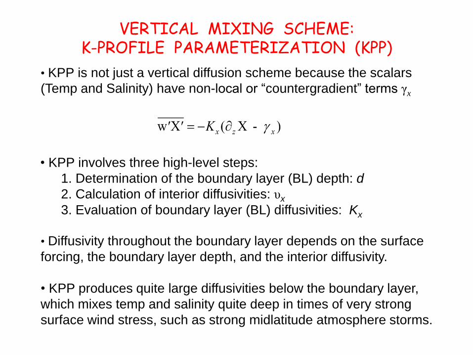
• KPP is not just a vertical diffusion scheme because the scalars
(Temp and Salinity) have non-local or “countergradient” terms γx
• KPP involves three high-level steps:
1. Determination of the boundary layer (BL) depth: d
2. Calculation of interior diffusivities: υx
3. Evaluation of boundary layer (BL) diffusivities: Kx
• Diffusivity throughout the boundary layer depends on the surface
forcing, the boundary layer depth, and the interior diffusivity.
• KPP produces quite large diffusivities below the boundary layer,
which mixes temp and salinity quite deep in times of very strong
surface wind stress, such as strong midlatitude atmosphere storms.
VERTICAL MIXING SCHEME:K-PROFILE PARAMETERIZATION (KPP)
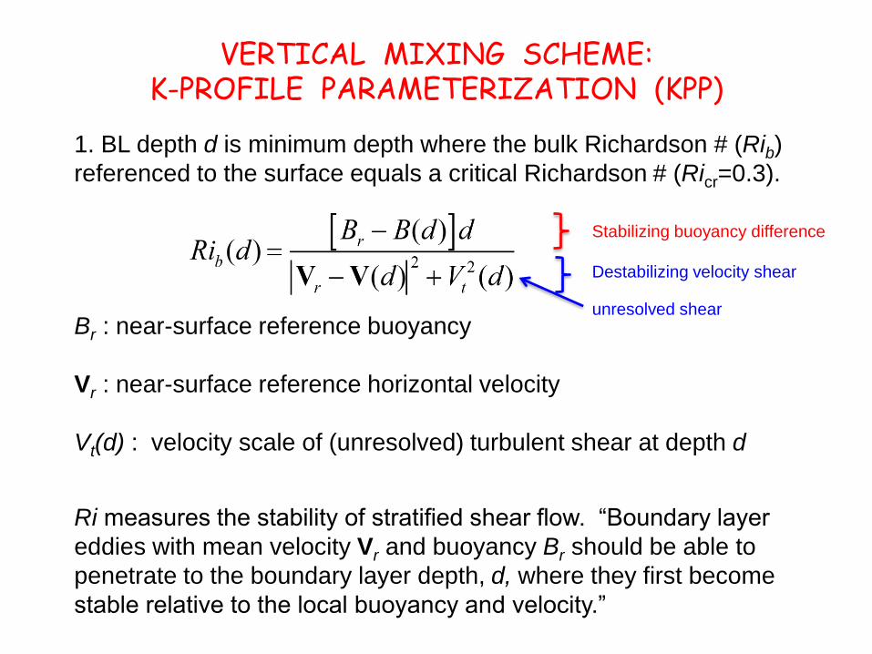
1. BL depth d is minimum depth where the bulk Richardson # (Rib)
referenced to the surface equals a critical Richardson # (Ricr=0.3).
Stabilizing buoyancy difference
Destabilizing velocity shear
Br : near-surface reference buoyancy
Vr : near-surface reference horizontal velocity
Vt(d) : velocity scale of (unresolved) turbulent shear at depth d
Ri measures the stability of stratified shear flow. “Boundary layer
eddies with mean velocity Vr and buoyancy Br should be able to
penetrate to the boundary layer depth, d, where they first become
stable relative to the local buoyancy and velocity.”
unresolved shear
VERTICAL MIXING SCHEME:K-PROFILE PARAMETERIZATION (KPP)
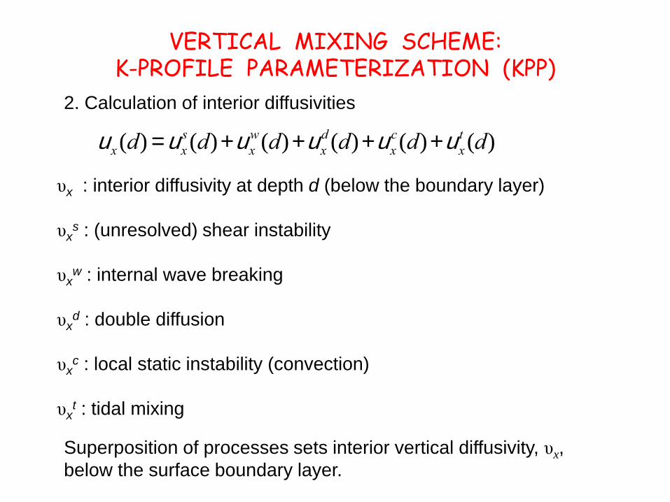
2. Calculation of interior diffusivities
υx : interior diffusivity at depth d (below the boundary layer)
υxs : (unresolved) shear instability
υxw : internal wave breaking
υxd : double diffusion
υxc : local static instability (convection)
υxt : tidal mixing
Superposition of processes sets interior vertical diffusivity, υx,
below the surface boundary layer.
ux(d) =uxs(d)+ux
w(d)+uxd (d)+ux
c(d)+uxt (d)
VERTICAL MIXING SCHEME:K-PROFILE PARAMETERIZATION (KPP)
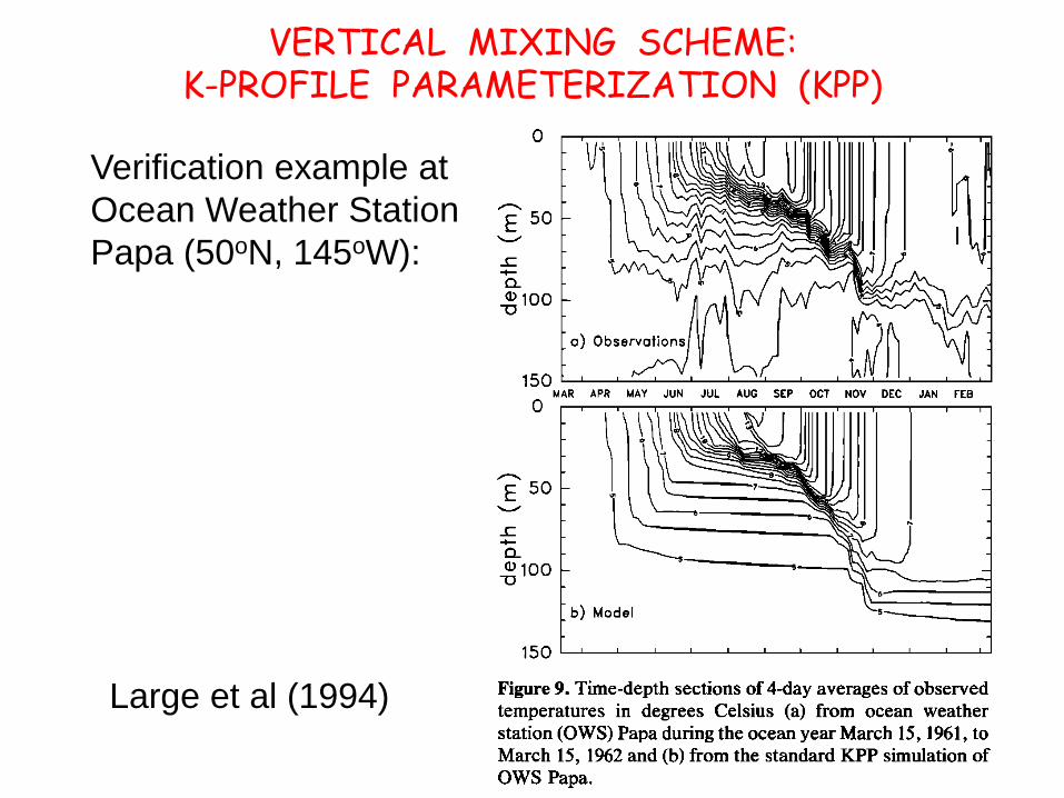
Verification example at
Ocean Weather Station
Papa (50oN, 145oW):
Large et al (1994)
Lateral Mixing (Interior, Tracer Diffusion)
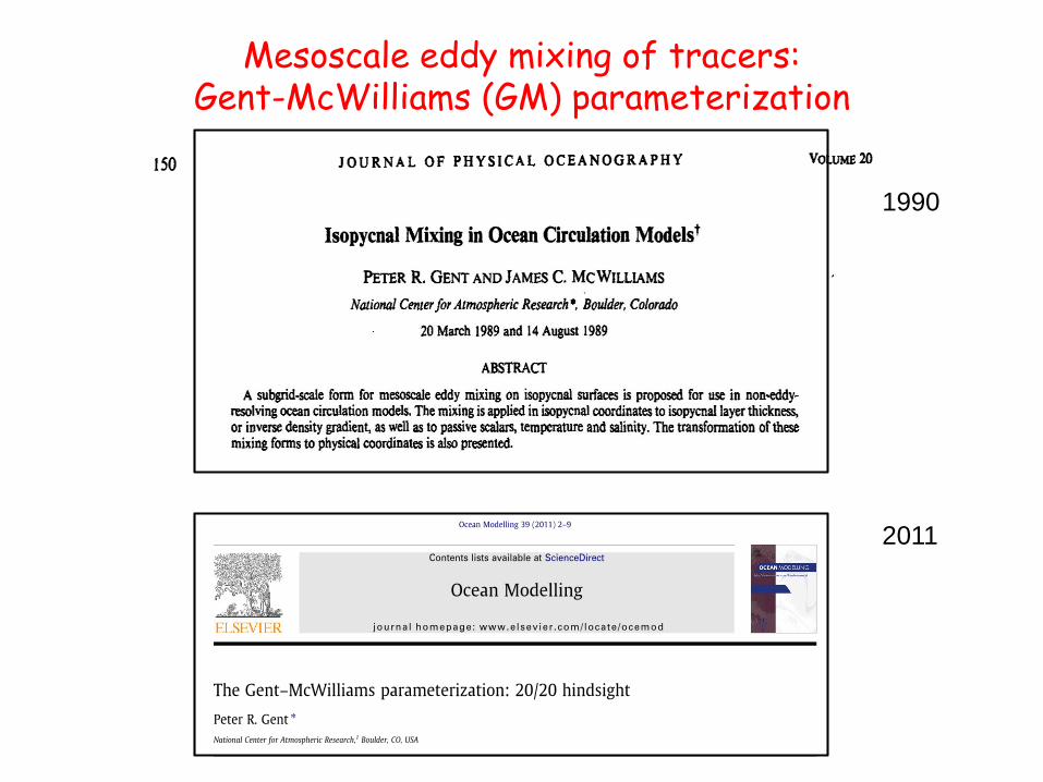
Mesoscale eddy mixing of tracers:Gent-McWilliams (GM) parameterization
1990
2011

GFDL climate model with ocean resolution of 0.1o
Lateral Mixing (Interior, Tracer Diffusion)
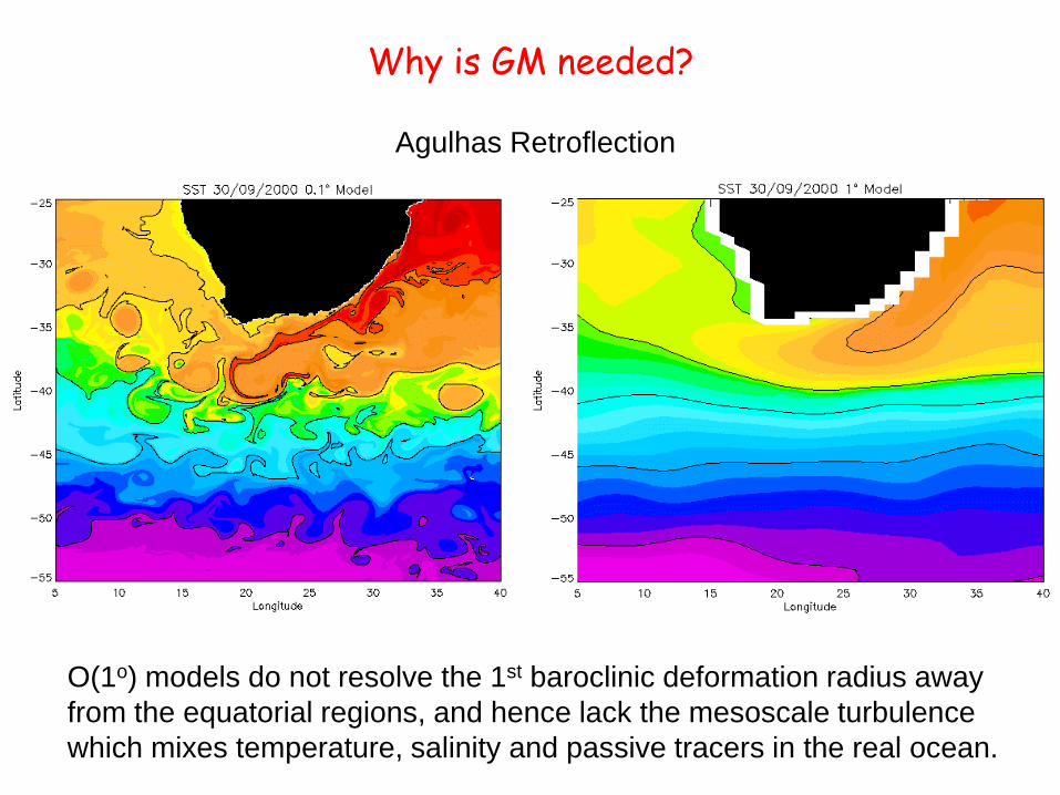
Why is GM needed?
O(1o) models do not resolve the 1st baroclinic deformation radius away
from the equatorial regions, and hence lack the mesoscale turbulence
which mixes temperature, salinity and passive tracers in the real ocean.
Agulhas Retroflection

ISOPYCNAL
(r=constant)
DEPTH
Ocean Observations suggest mixing along isopycnals
is ~107 times larger than across isopycnals.
• Early ocean models parameterized the stirring effects of (unresolved)
mesoscale eddies by Laplacian horizontal diffusion with KH = O(103 m2/s),
whereas the vertical mixing coefficient Kv = O(10-4 m2/s).
• Horizontal mixing results in excessive diapycnal mixing, which degrades the
ocean solution: e.g. Veronis (1975) showed that it produces spurious upwelling
in western boundary current regions which “short circuits” the N. Atlantic MOC.
• Thus, was a recognized need to orient tracer diffusion in z-coordinate models
along isopycnal surfaces, to be consistent with observed ocean mixing rates.
Why is GM needed?
Isopycnal slopes
are small O(10-3)
at most

The GM Parameterization
TTuut
T
2*).(
.0*.),/.(* uw z
GM (1990) proposed an eddy-induced velocity u* in addition to diffusion along isopycnal surfaces.
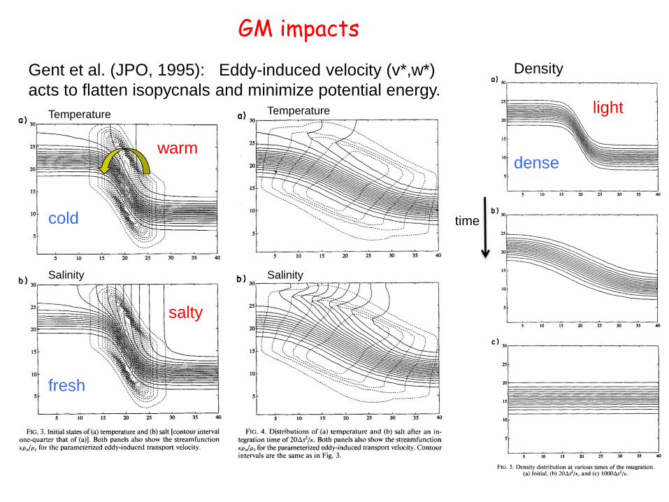
GM impacts
Gent et al. (JPO, 1995): Eddy-induced velocity (v*,w*)
acts to flatten isopycnals and minimize potential energy.
warm
cold
salty
fresh
light
dense
Temperature
Salinity
Temperature
Density
Salinity
time
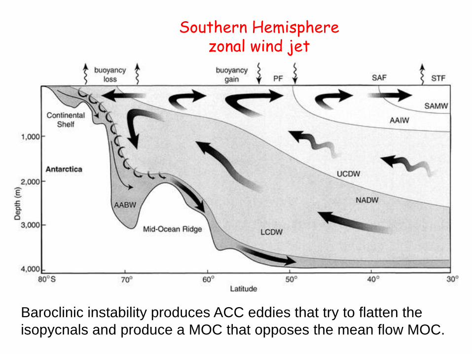
Southern Hemisphere zonal wind jet
Baroclinic instability produces ACC eddies that try to flatten the
isopycnals and produce a MOC that opposes the mean flow MOC.
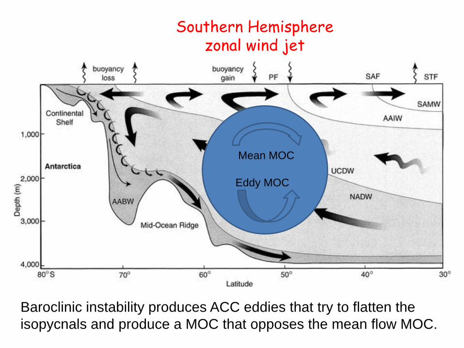
Southern Hemisphere zonal wind jet
Mean MOC
Eddy MOC
Baroclinic instability produces ACC eddies that try to flatten the
isopycnals and produce a MOC that opposes the mean flow MOC.

Danabasoglu et al. (1994, Science)
4o x 3o x 20L ocean model
Impacts of GM
(a) Horizontal Diffusion, MOC (u)
(b) GM, MOC (u)
(c) GM, MOC (u+u*)

Danabasoglu et al. (1994, Science)
4o x 3o x 20L ocean model
Impacts of GM
(a) Horizontal Diffusion
(b) GM
Deep Water Formation
In (b), deep water is formed
only in the Greenland/
Iceland/Norwegian Sea, the
Labrador Sea, the Weddell
Sea and the Ross Sea.

Mimics effects of unresolved mesoscale eddies as the sum of
- diffusive mixing of tracers along isopycnals (Redi 1982),
- an additional advection of tracers by the eddy-induced velocity u*
Scheme is adiabatic and therefore valid for the ocean interior.
Acts to flatten isopycnals, thereby reducing potential energy.
Eliminates any need for horizontal diffusion in z-coordinate OGCMs
eliminates Veronis effect.
Implementation of GM in ocean component was a major factor enabling
stable coupled climate model simulations without “flux adjustments”.
GM summary

Limerick 2004
There
There once was an ocean model called POP,
Which occasionally used to flop,
But eddy advection, and much less convection,
Turned it into the cream of the crop.