obtaining new local minima in lens design by constructing

Obtaining new local minima in lens design by constructing saddle points

Maarten van Turnhout,1 Pascal van Grol,1 Florian Bociort,2,* and H. Paul Urbach2 1TNO, Stieltjesweg 1, 2628 CK Delft, The Netherlands

2Faculty of Applied Sciences, Delft University of Technology, Lorentzweg 1, 2628 CJ Delft, The Netherlands *[email protected]

Abstract: We show that in the lens design landscape saddle points exist that are closely related to local minima of simpler problems. On the basis of this new theoretical insight we develop a systematic and efficient saddle-point method that uses a-priori knowledge for obtaining new local minima. In contrast with earlier saddle-point methods, the present method can create both positive and negative lenses. As an example, by successively using the method a good-quality local minimum is obtained from a poor-quality one. The method could also be applicable in other global optimization problems that satisfy the requirements discussed in this paper.

©2015 Optical Society of America

OCIS codes: (080.2720) Mathematical methods (general); (220.2740) Geometric optical design; (220.3620) Lens system design.

References and links

1. H. Gross, H. Zügge, M. Peschka, and F. Blechinger, Handbook of Optical Systems (Wiley-VCH, 2007), Vol. 3. 2. F. Bociort, “Optical system optimization, ”in Encyclopedia of Optical Engineering (Marcel Dekker, 2003). 3. T. G. Kuper and T. I. Harris, “Global optimization for lens design - an emerging technology,” Proc. SPIE 1780,

14–28 (1992). 4. G. W. Forbes and A. E. Jones, “Towards global optimization with adaptive simulated annealing,” Proc. SPIE

1354, 144–153 (1991). 5. M. Isshiki, H. Ono, K. Hiraga, J. Ishikawa, and S. Nakadate, “Lens design: Global optimization with Escape

Function,” Opt. Rev. 2(6), 463–470 (1995). 6. K. E. Moore, “Algorithm for global optimization of optical systems based on genetic competition,” Proc. SPIE

3780, 40–47 (1999). 7. L. W. Jones, S. H. Al-Sakran, and J. R. Koza, “Automated synthesis of both the topology and numerical

parameters for seven patented optical lens systems using genetic programming,” Proc. SPIE 5874, 587403 (2005).

8. D. Shafer, “Global optimization in optical design,” Comput. Phys. 8(2), 188–195 (1994). 9. J. R. Rogers, “Using global synthesis to find tolerance-insensitive design forms,” Proc. SPIE 6342, 63420M

(2006). 10. F. Bociort, E. van Driel, and A. Serebriakov, “Networks of local minima in optical system optimization,” Opt.

Lett. 29(2), 189–191 (2004). 11. E. van Driel, F. Bociort, and A. Serebriakov, “Topography of the merit function landscape in optical system

design,” Proc. SPIE 5249, 353–363 (2004). 12. F. Bociort, A. Serebriakov, and M. van Turnhout, “Saddle points in the merit function landscape of systems of

thin lenses in contact,” Proc. SPIE 5523, 174–184 (2004). 13. F. Bociort and M. van Turnhout, “Looking for order in the optical design landscape,” Proc. SPIE 6288, 628806

(2006). 14. O. Marinescu and F. Bociort, “Network search method in the design of extreme ultraviolet lithographic

objectives,” Appl. Opt. 46(35), 8385–8393 (2007). 15. F. Bociort and M. van Turnhout, “Saddle points reveal essential properties of the merit-function landscape,”

SPIE Newsroom (2008), http://spie.org/x31524.xml?highlight=x2422&ArticleID=x31524F. 16. P. van Grol, F. Bociort, and M. van Turnhout, “Finding order in the design landscape of simple optical systems,”

Proc. SPIE 7428, 742808 (2009). 17. F. Bociort and M. van Turnhout, “Finding new local minima in lens design landscapes by constructing saddle

points,” Opt. Eng. 48(6), 063001 (2009). 18. D. Dilworth, “Novel global optimization algorithms: binary construction and the saddle-point method,” Proc.

SPIE 8486, 84860A (2012). 19. N. Mousseau and G. T. Barkema, “Travelling through potential energy landscapes of disordered materials: The

activation-relaxation technique,” Phys. Rev. E Stat. Phys. Plasmas Fluids Relat. Interdiscip. Topics 57(2), 2419–2424 (1998).

#229182 - $15.00 USD Received 8 Dec 2014; revised 24 Feb 2015; accepted 25 Feb 2015; published 3 Mar 2015 © 2015 OSA 9 Mar 2015 | Vol. 23, No. 5 | DOI:10.1364/OE.23.006679 | OPTICS EXPRESS 6679

20. G. Wei, N. Mousseau, and P. Derreumaux, “Exploring the energy landscape of proteins: A characterization of the activation relaxation technique,” J. Chem. Phys. 117(24), 11379 (2002).

21. D. J. Wales, Energy Landscapes (Cambridge University, 2003). 22. J. P. K. Doye and D. J. Wales, “Surveying a potential energy surface by eigenvector-following applications to

global optimization and the structural transformations of clusters,” Zeitschrift Phys. D 40(1-4), 194–197 (1997). 23. E. W. Weisstein, “Cayley Cubic”, From MathWorld-A Wolfram Web Resource,

http://mathworld.wolfram.com/CayleyCubic.html. 24. F. Bociort, “Why are there so many system shapes in lens design?” Proc. SPIE 7849, 78490D (2010). 25. I. Livshits, Z. Hou, P. van Grol, Y. Shao, M. van Turnhout, P. Urbach, and F. Bociort, “Using saddle points for

challenging optical design tasks,” Proc. SPIE 9192, 919204 (2014). 26. O. Marinescu and F. Bociort, “Saddle-point construction in the design of lithographic objectives, part 1:

method,” Opt. Eng. 47(9), 093002 (2008). 27. O. Marinescu and F. Bociort, “Saddle-point construction in the design of lithographic objectives, part 2:

application,” Opt. Eng. 47(9), 093003 (2008). 28. E. W. Weisstein, “Bisection”, From MathWorld-A Wolfram Web Resource,

http://mathworld.wolfram.com/Bisection.html. 29. C. Wang, Master Thesis, (TU Delft, 2006). 30. M. van Turnhout and F. Bociort, “Instabilities and fractal basins of attraction in optical system optimization,”

Opt. Express 17(1), 314–328 (2009).

1. Introduction

One of the major challenges in the design of optical imaging systems and in other applications comes from the existence of many local minima in the merit function (MF) landscape. When these local minima are present, the solution that is obtained after local optimization is critically dependent on the choice of the initial configuration. Traditionally, the choice of the initial design configuration has been done on the basis of previous experience, patents, or databases (adapted to the new specifications), intuition, and often a considerable amount of trial and error [1, 2].

Over the past decades, the impressive increase in computer power raised the interest in developing global optimization methods that have the capability to overcome the MF barriers between local minima [3–9]. For design tasks for which the complexity is not too high, present-day global optimization algorithms are valuable tools for finding good design solutions. However, with methods without a-priori knowledge (e.g. methods that rely only on generally applicable mathematical algorithms), the computational effort increases rapidly with the complexity of the design problem. Therefore, in the available time the design space is often insufficiently explored and potentially valuable design solutions can be missed.

To tackle this problem, an approach frequently used in practice is to start with known configurations and increase the complexity as necessary to solve the problem. In the same spirit, we show how certain properties of the MF landscape, combined with existing knowledge about designs that are simpler than the one envisaged, can be used to improve design productivity by making it possible to move rapidly between different local minima. The required properties of the MF landscape will be described in this paper in the specific context of lens design, but the general ideas could be useful in other applications as well. These properties can be understood when we consider not only local minima, but saddle points (SP’s) as well [10–16].

In lens design, we developed earlier a method to obtain saddle points by inserting a lens into an existing local minimum when the glass and insertion position of the new lens satisfy special conditions [17]. This special case of the so-called saddle-point construction (SPC) has become a practical design method and was recently implemented in the commercial lens design program SYNOPSYS (under the name SPBUILD) [18]. In this paper, we describe a general version of SPC, for which the glass and distance restrictions mentioned in [17] are removed. With the general SPC method, a broader diversity of new local minima can be found than with the special version.

In Sec. 2 we discuss the concept of SP and review well-known properties of these points. The basic idea of the general SPC technique is discussed in Sec. 3. Sections 2 and 3 do not use lens design concepts and could also be useful for readers interested in applications other than lens design. In Sec. 4 we show that to construct a SP in lens design the curvatures of the lens to be inserted can be computed with a simple one-dimensional numerical calculation.


Examples are given in Sec. 5. In Sec. 6 we illustrate how the SPC method can be used for practical purposes.

2. Saddle points

In the MF landscape, a design configuration with N optimization variables is a point in an N-dimensional space. The critical points in the landscape are the points for which the gradient of MF vanishes. If the matrix of the second-order derivatives of MF (i.e. the Hessian) with respect to the optimization variables has only nonzero eigenvalues, the critical point is called non-degenerate. An important characteristic of non-degenerate critical points is the number of negative eigenvalues of the Hessian, the so-called Morse index (MI). A negative eigenvalue indicates that the critical point is a maximum along the direction defined by the corresponding eigenvector of the Hessian. Therefore, minima have MI = 0, maxima have MI = N, and SP’s have MI values between 1 and N-1.

In an intuitive analogy we can think about the MF landscape as a mountain scenery, where the height at a certain position is the MF value of the corresponding configuration. There, the SPs are the mountain passes in the landscape. In two dimensions, a SP is a maximum in one direction (called the downward direction, indicated in Fig. 1(a) by the green curve) and a minimum along the other direction (red curve), which is perpendicular to the first one. In two dimensions all SP’s have MI = 1. Two-dimensional SP’s are connected to two minima, i.e. when we choose for local optimization two starting points close to each other, but on opposite sides of the saddle, they will lead to two distinct minima after optimization [Fig. 1(b)].

Fig. 1. a) Saddle point in a MF landscape with two variables var1 and var2. b) Optimization on both sides of the saddle leads to two distinct local minima.

Saddle points that are connected with only two minima are particularly useful. In the N-dimensional case, SP’s with MI = 1 have this property. They have one downward direction, and they are minima in all directions perpendicular to the downward one. Intuitively, the downward direction of an N-dimensional SP with MI = 1 is similar to the downward direction of a two-dimensional saddle point. When certain quite general conditions are met, in global searches with a fixed number of variables all minima are connected in a network. In this network, each link between minima contains a SP with MI = 1 [10–14]. The network for a certain region of interest in the design space can be found link by link, by detecting for each minimum the SP’s with MI = 1 that are connected to it, and then by repeating the procedure for the new minima found on the other side of the SP’s that have been detected. For global searches that are sufficiently simple, e.g. for the search corresponding to the well-known Cooke triplet [10], the entire network can be found in this way. However, when the number of components increases, detecting SP’s with MI = 1 without a-priori knowledge of the MF landscape [10,11,14, 19–22] becomes time-consuming. In this paper we show that in certain global optimization problems a-priori knowledge does exist. By using an intrinsic property present in the lens design landscape (and perhaps elsewhere as well), the existence of so-


called “null” elements with at least two variables, as discussed in the next section, we develop a method to obtain SP’s with MI = 1 from simpler known minima that is computationally much more effective: saddle-point construction (SPC).

In preparation for the discussion of the basic idea of the general SPC method, Fig. 2 shows the well-known shapes of equimagnitude hypersurfaces (i.e. the hypersurfaces on which the MF is constant) in the vicinity of SP’s with MI = 1. Figure 2a shows that for a MF value that is slightly larger than the merit function value MFSP of the SP, the surface consists of one piece.

Figure 2(b) shows the typical conical shape of the equimagnitude surface when MF = MFSP. The SP with MI = 1 is the top of the double conic surface. At larger distances from the SP the (hyper)surface will deviate from the conical shape, but the essential fact that will be used in the next section is that the two parts have a common point, the SP.

Fig. 2. Shapes of the MF equimagnitude surfaces close to the SP with MI = 1. a) MF > MFSP, b) MF = MFSP, c) MF < MFSP . At very small distances from the SP, where the MF can be accurately described by a quadratic approximation, these surfaces become a hyperboloid with one sheet, a double cone with the SP at the common top and a hyperboloid with two sheets, respectively. The properties shown here in a three-dimensional space are generally valid in the N-dimensional case.

Fig. 3. In a plane, the SP is located at the crossing point of two equimagnitude lines. The thick line is oriented along the eigenvector with negative eigenvalue.

Figure 2(c) shows the equimagnitude surface corresponding to a MF value that is slightly lower than that of the SP. Note that the surface splits into two separate parts. Figure 2(c) also shows the shortest line that can connect the two parts. Along this line the saddle point SP is a maximum. This line (called above the downward direction), corresponds to the direction of the most rapid decrease of the MF, and is oriented along the unique eigenvector of the Hessian matrix at the SP that has negative eigenvalue. Since the MI is 1, in any direction perpendicular to this direction and passing through SP, the SP is a minimum.

In any two-dimensional plane passing through the downward direction (the thick line in Fig. 3), the equimagnitude lines corresponding to MFSP are two lines crossing at the SP, as in the case of a two-dimensional saddle point.


3. Constructing saddle points

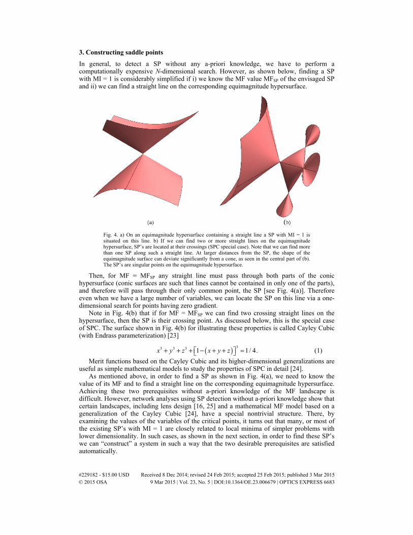
In general, to detect a SP without any a-priori knowledge, we have to perform a computationally expensive N-dimensional search. However, as shown below, finding a SP with MI = 1 is considerably simplified if i) we know the MF value MFSP of the envisaged SP and ii) we can find a straight line on the corresponding equimagnitude hypersurface.

Fig. 4. a) On an equimagnitude hypersurface containing a straight line a SP with MI = 1 is situated on this line. b) If we can find two or more straight lines on the equimagnitude hypersurface, SP’s are located at their crossings (SPC special case). Note that we can find more than one SP along such a straight line. At larger distances from the SP, the shape of the equimagnitude surface can deviate significantly from a cone, as seen in the central part of (b). The SP’s are singular points on the equimagnitude hypersurface.

Then, for MF = MFSP any straight line must pass through both parts of the conic hypersurface (conic surfaces are such that lines cannot be contained in only one of the parts), and therefore will pass through their only common point, the SP [see Fig. 4(a)]. Therefore even when we have a large number of variables, we can locate the SP on this line via a one-dimensional search for points having zero gradient.

Note in Fig. 4(b) that if for MF = MFSP we can find two crossing straight lines on the hypersurface, then the SP is their crossing point. As discussed below, this is the special case of SPC. The surface shown in Fig. 4(b) for illustrating these properties is called Cayley Cubic (with Endrass parameterization) [23]

( ) 33 3 3 1 1/ 4.x y z x y z+ + + − + + = (1)

Merit functions based on the Cayley Cubic and its higher-dimensional generalizations are useful as simple mathematical models to study the properties of SPC in detail [24].

As mentioned above, in order to find a SP as shown in Fig. 4(a), we need to know the value of its MF and to find a straight line on the corresponding equimagnitude hypersurface. Achieving these two prerequisites without a-priori knowledge of the MF landscape is difficult. However, network analyses using SP detection without a-priori knowledge show that certain landscapes, including lens design [16, 25] and a mathematical MF model based on a generalization of the Cayley Cubic [24], have a special nontrivial structure. There, by examining the values of the variables of the critical points, it turns out that many, or most of the existing SP’s with MI = 1 are closely related to local minima of simpler problems with lower dimensionality. In such cases, as shown in the next section, in order to find these SP’s we can “construct” a system in such a way that the two desirable prerequisites are satisfied automatically.


The required a-priori knowledge for this approach is a minimum (its merit function is denoted by MF0) in a design space with lower dimensionality. To this minimum we add what we call a “null” element, with which we increase the dimensionality of the MF landscape in a way that does not change the value of the MF, i.e. we keep MF = MF0. In the version of the method discussed in this paper, the null element has two coupled variables, such that varying them corresponds to a straight line on the equimagnitude surface having MF = MF0. Along this line we search for points with zero gradient. If such a point is non-degenerate, it is a SP. This technique will be called SPC in the general case. After the SP is found, the null-element variables are decoupled and become independent, and optimization on both sides of the SP leads to two minima, as shown in Fig. 1(b). In the next section we show how this technique can be applied in lens design. For readers interested in other applications, the discussion in the next section provides a specific example that helps to clarify details of SPC that could be of more general interest.

4. Generalizing the SPC method in lens design

We discuss below the SPC method in the case of lens systems with spherical surfaces. For simplicity, for SPC the optimization variables are only the surface curvatures. The method can be generalized to mirrors and aspherical surfaces, as shown for the special case of SPC [26, 27]

We start with an optical system with N surfaces that is already a local minimum in all variables (these will be called in what follows the “old” variables, and will be collected in the vector 0c

). In this system we insert a lens in such a way that we create a saddle point, as

described below. First, in the original minimum we insert two new surfaces with the same curvature and zero distance between them [Fig. 5]. The pair of surfaces form either a lens meniscus, or an air meniscus (e.g. by splitting an existing lens). With zero distance and equal curvatures, the pair of surfaces disappear optically (i.e. this pair is the “null” element) and does not affect the path of any ray. Therefore, for any value of the common curvature of the new surfaces, the MF remains equal to MF0, the value for the original minimum with N surfaces.

Fig. 5. Inserting a “null” element in an existing local minimum i) leaves the MF unchanged and ii) creates a straight line on the corresponding equimagnitude surface. A null element has two variables (in lens design, the two curvatures), such that when one variable changes the MF, the other one can restore the MF to the value corresponding to the old minimum (MF0).

If the two new surfaces have the indices k + 1 and k + 2 in the system, their curvatures are

1kc + and 2kc + and the transformation

0 1 2 0 1 2( , , ) ,k k k kMF c c c MF c c+ + + += = with (2)

where 1kc + is variable and 0c

is constant, defines a line on the equimagnitude hypersurface with MF = MF0. Note that because Eq. (2) defines a linear transformation, the corresponding line in the variable space is straight.

We have shown earlier [17] how saddle points can be constructed in the special case when the inserted lens is in direct contact with one of the surfaces of the original local minimum (called below the reference surface) and when the glass of the new lens is the same as that at the reference surface. We have then three successive surfaces with two zero axial distances between them, and two transformations that leave the MF unchanged, i.e. MF = MF0. One


transformation corresponds to a glass meniscus of arbitrary curvature, the other one to an air meniscus. The two corresponding straight lines on the equimagnitude hypersurface with MF = MF0 have an intersection point when the two new curvatures are equal to the one of the reference surface (having index k)

1 2k k kc c c+ += = . (3)

If, as typically is the case, this point is non-degenerate, it is a SP. In the general version of the SPC method, the glass and insertion position can be arbitrary,

but the curvature 1kc + ( = 2kc + ) that leads to a saddle point must be computed numerically. The general version of SPC was described by us in a preliminary form (unrefereed) in [13]. The detailed description is given in this paper.

For finding the condition that leads to a SP, we define the auxiliary variables

1 2 2 1( ) / 2, ( ) / 2k k k kc c c cξ η+ + + += + = − . (4)

For 0η = , each value (within a suitable range) of the variableξ defines a point on the

straight line on the equimagnitude hypersurface. Using 1 2,k kc cξ η ξ η+ += − = + and writing

0 0( , , ) ( , , )f c MF cξ η ξ η ξ η= − + (5)

it follows from Eq. (2) that 0 0( , , 0)f c MF const for allξ η ξ= = = and therefore we have

0( , , 0) 0 . f c for allξ η ξξ∂ = =

∂

(6)

The partial derivatives of the merit function with respect to the old optimization variables remain unchanged, i.e. equal to zero. Critical points are then zeros of the remaining derivative considered now to be a function only of ξ , i.e. values 0ξ such that

0 0 0( , , ) 0 .f c ηξ η

η =

∂ =∂

(7)

Then for the curvature of the null element 1, 2, 0s k s k sc c c ξ+ += = = we have a critical point.

If it is non-degenerate, because we have added to a minimum only two variables, the MI of this critical point cannot be larger than two. It cannot be zero (i.e. a local minimum) because for local minima the equimagnitude hypersurfaces of MF around them are ellipsoids that reduce to a single point when MF has the value that corresponds to the minimum. However, for solutions of Eq. (7) the corresponding MF remains constant on an entire straight line ( 0η = ). In all cases we have examined so far, we have used a paraxial equality constraint (the focal length or the total track was kept constant) and we have numerically determined a MI of one. We call a SP constructed with SPC a “null-element” SP (NESP).

Equivalent to the conditions in Eqs. (6) and (7) is the requirement that the partial derivatives 1/ kMF c +∂ ∂ and 2/ kMF c +∂ ∂ must vanish at the SP. Since along the line 0η = we have

1 21 2

d d d 0k kk k

MF MFMF c c

c c+ ++ +

∂ ∂= + =∂ ∂

(8)

and 1 2d dk kc c+ += , it follows that

1 2k k

MF MF

c c+ +

∂ ∂= −∂ ∂

(9)


which means that both new components of the gradient vanish simultaneously. Thus, for finding the saddle points, it is sufficient to find numerically the values of 1kc + , considered now as the only variable, for which:

1

0 .k

MF

c +

∂ =∂

(10)

The derivative in Eq. (10), satisfying the condition in Eq. (2), can be computed numerically as

1 1 1 1

1

( , ) ( , )

2k k k k

k

MF c c c MF c c cMF

c c+ + + +

+

+ Δ − − Δ∂ ≈∂ Δ

(11)

where cΔ is a small curvature change. It must be emphasized that in the computation of the derivative (11) existing equality constraints must be taken into account. If such constraints are present, and they are already satisfied in the original minimum, they are also satisfied when a null element is inserted. However, when for the computation of the MF derivative 1kc + is

replaced by 1kc c+ ± Δ , these constraints are in general affected. Therefore, before the MF in Eq. (11) is calculated, the constraints must be restored, e.g. with a “constraints-only” reoptimization for the “old” variables or by other means. Paraxial equality constraints implemented as a “solve” (e.g. constant effective focal length) are satisfied automatically in this case and do not require this extra step.

Equation (10) is an equation with only one unknown 1kc + that must be solved

numerically. In our numerical implementation, 1/ kMF c +∂ ∂ is first evaluated with Eq. (11) for

a set of equidistant values of 1kc + and then when 1/ kMF c +∂ ∂ changes sign between two

neighbouring points the value of 1kc + that leads to the SP is accurately determined with the well-known bisection root-finding method [28]. This technique is considerably more efficient than detecting a SP without a-priori knowledge.

The resulting SP has a downward direction in the MF space, shown in Fig. 1(a) by the green curve, and a new upward direction similar to the red curve. Along the downward direction, the new system is a maximum. When a NESP is found, we take for instance on the line given by Eq. (2) two points on opposite sides of the saddle, having:

1 2 ,k k sc c c ε+ += = ± (12)

where ε indicates a small curvature change. Then, these two points are optimized and two different local minima will result [see Fig. 1(b)]. At this stage, it is desirable to temporarily allow small edge-thickness violations for the null-element surfaces. In the resulting minima, any standard lens design procedure can be applied, e.g. other optimization variables can be added and the small edge-thickness violations mentioned above can be corrected. Also, the zero distance between surfaces k + 1 and k + 2, that was kept constant during SPC, can be increased to the desired values, for instance by increasing the zero distance in small steps, and by optimizing the obtained system after each step.

The general version of SPC can find local minima that cannot be found with the special version. For instance, in the next Section a NESP with a “null-air” lens that splits a doublet lens into two lenses will be used to obtain the strong negative lens in the well-known Cooke triplet design shape.

The SPC method can also be used in reverse order to extract a lens from an optical system (see Sec. 6). First, the distance between the two surfaces of the lens to be extracted should be made equal to zero. This should be done in small steps to prevent unpredictable jumps of the optimization algorithm. As in the case of increasing the zero distances, we keep the distances constant during optimization. When the distance between the two lens surfaces is zero, we make the curvatures of the resulting thin lens equal, which gives us a null-element meniscus


that can be easily extracted from the system without changing the MF. The reverse SPC method was implemented in the commercial lens design program SYNOPSYS as a method for automatic element deletion [18].

5. Examples

We have implemented and tested the general SPC method using Eqs. (10-12) in the macro languages of the optical design programs CODE V and Zemax. In all examples shown in this paper, we use CODE V and the MF is the CODE V default error function based on the transverse ray aberration computed with respect to the chief ray. Two examples of SPC for triplet lens systems are shown in Fig. 6. The system specifications and numbering are the same as in the Cooke triplet network in Fig. 3 of [10]. The notation si-j for a saddle point means that it is connected to the minima mi and mj.

As in the case shown in Fig. 4(b), the general SPC method typically finds more than one NESP for a certain position of the inserted null element. In Fig. 6(a) 3/MF c∂ ∂ is plotted as a

function of 3 4( )c c= for a doublet local minimum, in which a null element with curvatures

3c and 4c has been inserted after the first lens. The parabolic curve cuts the horizontal axis in two points. The reason for the existence of these two NESP solutions can be understood by examining their drawings: the two NESPs are closely related to NESPs existing in special cases of SPC for which surfaces 2 and 5 respectively are used as reference surfaces. The null element is placed at a finite distance from the neighboring surfaces and its glass differs from the glasses of the first and last lens. Despite of these facts, the drawings of the systems corresponding to the two saddle points s10-7 and s4-10 show that the null-element curvatures are almost the same as 2c and 5c , respectively. In fact, if for s10-7 the distance between the second and third surface is gradually decreased to zero, and the glass of the null element is gradually changed into the glass of the first lens, then it turns out that the saddle point has three consecutive equal curvatures [ 3 4 2c c c= = , as predicted by Eq. (3)]. Similarly, s4-10

can be continuously transformed into a “special case” NESP with 3 4 5c c c= = . From the two NESP’s, three local minima m4, m7 and m10 are obtained by optimizing the

systems resulting from Eq. (12) . Note that on one side both saddle points are connected to m10. When the zero lens thickness is increased, the three minima become the systems indicated by black arrows after re-optimization. The same three nonzero thickness minima (m4, m7 and m10) can also be obtained with our SP detection software [11], together with two nonzero thickness saddle points (s10-7 and s4-10) linked to them.

By comparing the NESPs with the corresponding nonzero thickness SPs [the red boxes in Fig. 6(a)], we observe that with the exception of the thickness of the middle lens the shapes of the systems are essentially identical. Thus, the fact that one lens in the SP constructed with this method has zero thickness is not an obstacle for theoretical analysis or practical applications, because from NESPs the same minima with nonzero thickness can be obtained as from the corresponding nonzero thickness saddle points. It is just technically easier to increase the thickness in a local minimum than in a saddle point. However, the use of a zero-thickness null element in SPC has generated the straight line on the equimagnitude surface (having the MF of the start doublet) that made the one-dimensional search for NESPs possible. In contrast, for finding SP’s in which all lenses and airspaces have finite thickness, computationally expensive N-dimensional detection techniques must be used. Because they are closely related to NESPs, finite-thickness SP’s like the two SP’s in the dashed box in Fig. 6(a) will be called quasi-NESPs (QNESPs). We expect SPC to be useful in landscapes where many, or most SP’s are NESPs or QNESPs.

Obtaining the three minima in Fig. 6(a) does not necessarily require the general version of SPC, the special SPC version is sufficient. However, Fig. 6(b) shows an example where the use of the general version of SPC is essential. Here we insert a null air lens into the first lens of a doublet. In this example, three saddle points are found. The SP s-extra is unstable (i.e. it disappears easily when specifications are changed) and is not found in the earlier search [10].


On one side, s-extra leads to m19, whereas on the other side optimization will result in ray error (a ray misses a surface). Note that via saddle point s2-3, we obtain the Cooke triplet m2. This system cannot be obtained from doublets with the special SPC version.

Fig. 6. Construction of triplet saddle points (red boxes) by inserting a null-element meniscus into a doublet local minimum with variable curvatures. The aperture, fields, wavelength specifications, and glass types are typical for a Cooke triplet global search with object at infinity. The minima are shown in blue boxes. (a) The glass null element is inserted between the two lenses of a doublet. The SPs in the dashed box are obtained with SP detection, their SPC counterparts with a zero-thickness null element are underlined. The three minima in the dashed box can be obtained both in a computationally expensive way via SP detection, or rapidly via SPC (b) The null element has air between its surfaces, and is inserted in the middle of the first lens of a doublet.

The earlier special version of SPC cannot create strong negative lenses directly. Therefore, the ability of the general method of SPC to produce not only positive, but negative lenses (like the middle lens in a Cooke triplet) as well, is a significant improvement.

The shape of the 1/ kMF c +∂ ∂ -curve and the number of zeros of 1/ 0kMF c +∂ ∂ = depends on the starting local minimum, the position of the inserted null element, and the system parameters such as the entrance pupil diameter (EPD) and fields [29]. Figure 7 shows an example where four NESPs can be found in the same line search. In a local minimum with seven variable curvatures, a null-element meniscus has been inserted in contact with the first lens surface [see Fig. 7(a)]. The glass of the null element is the same as the glass of the first


lens of the old configuration. Note that in this case only one NESP can be constructed with the special version. In Fig. 7(b) 1/MF c∂ ∂ is plotted as a function of 1 2( )c c= . The curve cuts

the horizontal axis ( 1/ 0MF c∂ ∂ = ) in four points. The NESP corresponding to the third intersection point (indicated with the arrow) is the same as the one obtained by using the SPC method in the special case.

Fig. 7. a) Construction of saddle points by inserting a null element into a lens configuration with seven variables (EPD = 35 mm, fields are 0, 1.4 and 2 degrees, an effective focal length of 100 mm, and object at infinity, the last surface is used to keep the focal length constant).

The insert position is indicated by the dashed line. b)1

/MF c∂ ∂ -curve for the maximal range

of1

c . For larger absolute values, ray failure occurs.

The visualisation of SP’s in high-dimensional spaces is simple when the eigenvalues of the corresponding Hessian matrix are known. With the two new curvatures, the Hessian of each NESP in Fig. 7(b) has nine eigenvectors and eigenvalues. The lowest six eigenvalues, obtained with a Matlab code that communicates with CODE V, are listed for each NESP in Tab. 1. For all four NESPs, only one eigenvalue is negative, indicating that we have MI = 1. To facilitate the visualisation, we normalize separately for each NESP the set of eigenvalues such that the negative one has the value −1. Note that the absolute value of a positive eigenvalue can be larger or smaller than the absolute value of the negative eigenvalue.

Table 1. Six normalized eigenvalues for each of the SP’s in Fig. 7(b)

NESP Normalized eigenvalues1 −1. 0.3 1.8 4.6 8.9 69. 2 −1. 0.12 0.77 2.3 2.8 9.7 3 −1. 0.085 0.61 1.9 2.1 2.8 4 −1. 0.076 0.42 1.2 2.3 8.9

For each SP, its set of eigenvectors forms a new coordinate system in the variable space. If we choose from Tab.1 any positive eigenvalue λ, then in the plane defined by the corresponding eigenvector together with the downward direction (i.e. the eigenvector with the eigenvalue −1) the MF can be written as

2 2( , ) SPMF x y MF x yλ= + − (13)

where x and y are measured along the eigenvectors with eigenvalues λ and -l, respectively. The resulting plot is very similar to Fig. 1(a). Setting x = 0 and varying y corresponds to the green parabola in Fig. 1(a), while y = 0 and x variable corresponds to the red parabola, along which the SP is a minimum. A smaller value of λ leads to a flatter red parabola. For the remaining three large eigenvalues of each saddle point, that are not listed in Tab. 1, the MF increases very rapidly along the red parabola. With the same Matlab code it is possible to verify independently from the SPC calculations that the gradient vectors of the numerically computed NESPs have lengths very close to zero, as expected.


6. Using SPC for practical purposes

The set of initial configurations, which lead after local optimization to a given local minimum is called the “basin of attraction” of that minimum [30]. SP’s are always situated on the boundaries between different basins of attraction and can be used to switch the local optimization from one basin to a neighboring one. Since SPC requires only one-dimensional computations, it is computationally effective and has therefore the potential to become a useful tool for rapidly moving from one minimum to another one by successively inserting and extracting lenses in the design.

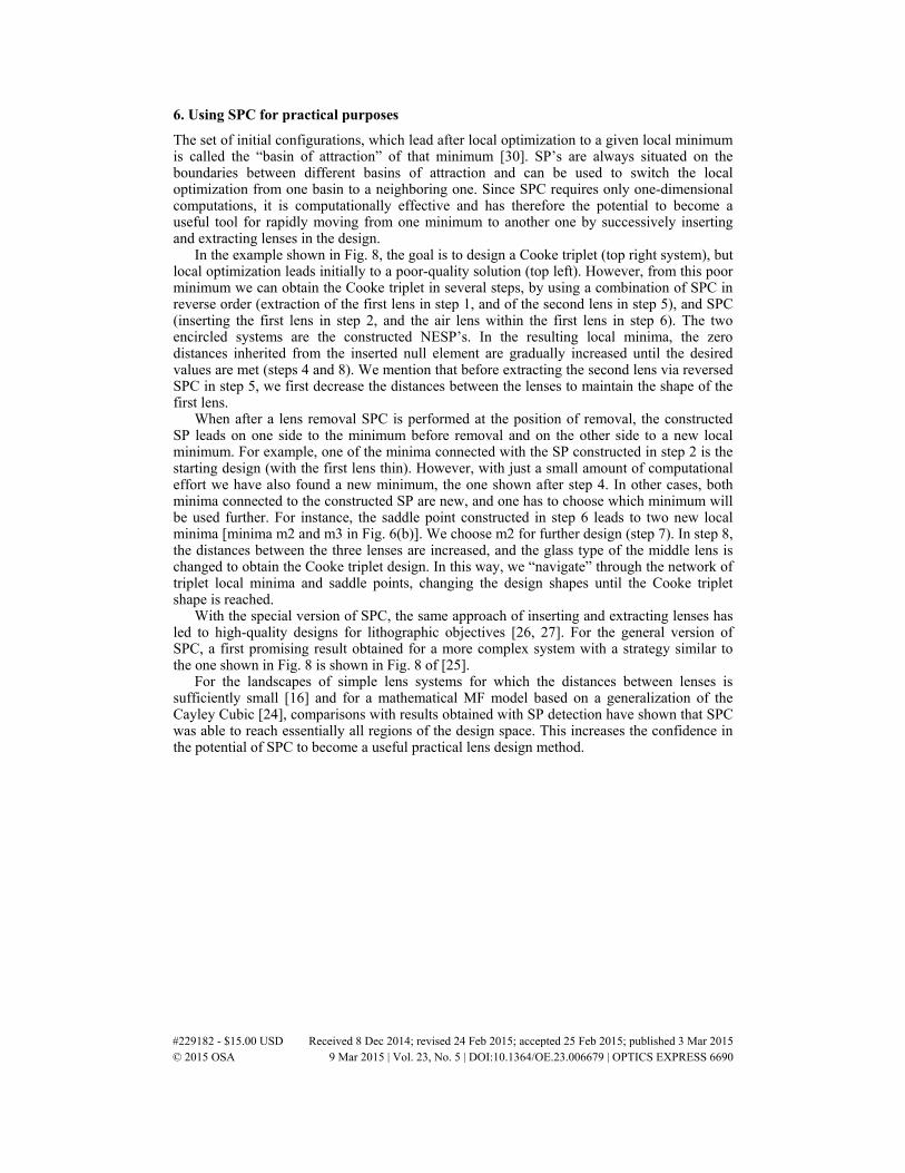
In the example shown in Fig. 8, the goal is to design a Cooke triplet (top right system), but local optimization leads initially to a poor-quality solution (top left). However, from this poor minimum we can obtain the Cooke triplet in several steps, by using a combination of SPC in reverse order (extraction of the first lens in step 1, and of the second lens in step 5), and SPC (inserting the first lens in step 2, and the air lens within the first lens in step 6). The two encircled systems are the constructed NESP’s. In the resulting local minima, the zero distances inherited from the inserted null element are gradually increased until the desired values are met (steps 4 and 8). We mention that before extracting the second lens via reversed SPC in step 5, we first decrease the distances between the lenses to maintain the shape of the first lens.

When after a lens removal SPC is performed at the position of removal, the constructed SP leads on one side to the minimum before removal and on the other side to a new local minimum. For example, one of the minima connected with the SP constructed in step 2 is the starting design (with the first lens thin). However, with just a small amount of computational effort we have also found a new minimum, the one shown after step 4. In other cases, both minima connected to the constructed SP are new, and one has to choose which minimum will be used further. For instance, the saddle point constructed in step 6 leads to two new local minima [minima m2 and m3 in Fig. 6(b)]. We choose m2 for further design (step 7). In step 8, the distances between the three lenses are increased, and the glass type of the middle lens is changed to obtain the Cooke triplet design. In this way, we “navigate” through the network of triplet local minima and saddle points, changing the design shapes until the Cooke triplet shape is reached.

With the special version of SPC, the same approach of inserting and extracting lenses has led to high-quality designs for lithographic objectives [26, 27]. For the general version of SPC, a first promising result obtained for a more complex system with a strategy similar to the one shown in Fig. 8 is shown in Fig. 8 of [25].

For the landscapes of simple lens systems for which the distances between lenses is sufficiently small [16] and for a mathematical MF model based on a generalization of the Cayley Cubic [24], comparisons with results obtained with SP detection have shown that SPC was able to reach essentially all regions of the design space. This increases the confidence in the potential of SPC to become a useful practical lens design method.


Fig. 8. Example of a design route from a poor local minimum (top left) to the Cooke triplet (top right) via SPC. The constructed saddle points are shown within circles.

7. Conclusion

In this paper we show that when the two conditions described in Sec. 3 are satisfied, saddle points exist in the design landscape that are closely related to local minima of simpler problems. On the basis of this new theoretical insight a method to find new minima in the landscape is developed. The SPC method presented in this paper uses a-priori knowledge for obtaining new local minima in the merit function landscape of optical systems. A known local minimum is transformed into a saddle point by inserting at any desired position a meniscus which does not affect the merit function of the known minimum. The values of the meniscus curvatures for which the resulting system is a saddle point are then computed with a simple one-dimensional calculation, that can be easily implemented in existing lens design software.

When we choose for local optimization two starting points close to each other, but on opposite sides of the saddle point, they will lead to two distinct minima after optimization, providing two possibilities for further design. By inserting and extracting lenses with the SPC method new local minima can be obtained rapidly. Due to its computational efficiency and systematic character, SPC has the potential to facilitate the search for high-quality solutions in the lens design landscape. Since in lens design both positive and negative lenses are needed, the ability of the general version of SPC to produce both types of lenses is essential for practical purposes.

SPC could also be applicable in other global optimization problems that satisfy the requirements discussed in Sec. 3. We expect SPC to be useful in landscapes where many, or most SP’s are NESPs or QNESPs.

Acknowledgments

The examples presented in this paper are obtained with an educational license of CODE V. We thank Zhe Hou and Chiung-tze Wang for testing the CODE V macro for the general SPC method. The Matlab code for computing eigenvalues for saddle points is written by Zhe Hou and includes modules written earlier by Thomas Liebig. Part of this research was supported by the Dutch Technology Foundation STW (Project No. 06817).


obtaining new local minima in lens design by constructing

Documents