On

Ia

b

c

d

a

ARRA

KNDHPLLO

1

wewnbcocbsubgtWr

D

(

1d

Chemical Engineering Journal 191 (2012) 243– 255

Contents lists available at SciVerse ScienceDirect

Chemical Engineering Journal

j ourna l ho mepage: www.elsev ier .com/ locate /ce j

bserver-based output feedback linearizing control strategy for aitrification–denitrification biofilter

. Torres Zúnigaa,d,∗, I. Queinnecb,c, A. Vande Wouwera

Service d’Automatique, Université de Mons, Boulevard Dolez 31, B-7000 Mons, BelgiumCNRS; LAAS; 7 avenue du Colonel Roche, F-31077 Toulouse, FranceUniversité de Toulouse; UPS, INSA, INP, ISAE; LAAS, F-31077 Toulouse, FranceDepartamento de Computación, Universidad del Papaloapan, Av. Ferrocarril s/n, Cd. Universitaria, 68400 Loma Bonita Oaxaca, Mexico

r t i c l e i n f o

rticle history:eceived 11 October 2011eceived in revised form 22 February 2012ccepted 2 March 2012

eywords:itrification–denitrification biofilter

a b s t r a c t

The objective of the present work is to propose an output-feedback control scheme for a wastewatertreatment biofilter, in order to regulate the outlet concentrations of nitrate and nitrite below a prescribedlevel (in accordance with the norms). The nitrification–denitrification biofilter is described by a set ofmass balance partial differential equations (PDEs), of hyperbolic or parabolic type, depending on theconsideration of diffusion/dispersion phenomena. The design of the output-feedback control strategyfollows a late lumping approach, in which the PDE system is considered, and descretized only at a later

istributed parameter systemsyperbolic PDEarabolic PDEinearizing controluenberger observerutput feedback control

stage for implementation purposes. This strategy is based on feedback linearization and requires a stateestimator, which takes the form of a distributed parameter Luenberger observer. A point of particularattention is the formulation of the model boundary conditions, from the classical Dankwerts conditions tomore advanced formulations including dynamic boundary conditions, which has a significant influenceon the control performance. The control strategy is tested against model uncertainties and measurementnoise in simulation.

. Introduction

Nitrate is a contaminant in groundwater aquifers and rivershich has been increasing in recent years mainly due to the

xtensive use of nitrogen fertilizers and improper treatment ofastewater from the industrial sites. Denitrification (reduction ofitrate nitrogen into nitrogen gas) is then an important step iniological wastewater removal systems. It may be classically pro-essed in full nitrification–denitrification activated sludge systemsr by biofiltration. Biofiltration is a technology based on a biologi-al reaction using micro-organisms which are immobilized formingiofilms or biolayers, where the bioreactions take place, aroundolid particles. These immobilized particles are packed in a col-mn known as a biofilter [1]. The development of biofiltration haseen promoted by its advantages over other alternative technolo-ies. It is an environmentally friendly and cost-effective method

hanks to its compactness, efficiency and low energy consumption.

ith the advent of more and more stringent norms for water reject,euse or for drinking water, the need for better understanding and

∗ Corresponding author at: Service d’Automatique, Université de Mons, Boulevardolez 31, B-7000 Mons, Belgium. Tel.: +32 65374130.

E-mail addresses: ixbalank@gmail.com (I. Torres Zúniga), queinnec@laas.frI. Queinnec), alain.vandewouwer@umons.ac.be (A. Vande Wouwer).

385-8947/$ – see front matter © 2012 Elsevier B.V. All rights reserved.oi:10.1016/j.cej.2012.03.011

© 2012 Elsevier B.V. All rights reserved.

improvement of reactor performance naturally comes to mind andimpels the development of efficient controllers to optimize thereal-time operation of these processes.

Many mathematical models of biofilters have been proposed tounderstand and improve the reactor performance [2]. Because thebiofilter state variables may be distributed both in time and space,a system of partial differential equations (PDE) is deduced from themass balance of each component (concentrations, biomass, etc.)to describe its dynamics. In this way, a biofilter is described as adistributed parameter system (DPS).

In order to control a DPS, two strategies are commonly used: theearly and late lumping approaches. In the first one, the partial dif-ferential equations are discretized to obtain an ordinary differentialequation (ODE) system and then, ODE-based control strategies fornonlinear or linear systems may be applied (see for example [3]).On the other hand, in the second approach, controllers are designedbased on the PDE model, and discretization occurs at a latter stageonly, so as to preserve the distributed nature of the problem as longas possible in the design procedure (see for example [4–6]).

For years, control of distributed parameter bioprocesses hasused the early lumping approach. This is because the most impor-

tant control strategies have been developed to control systemsdescribed by either linear or non-linear models represented byODEs. In this context, several works have been developed, forinstance: in [7], the authors applied adaptive control schemes to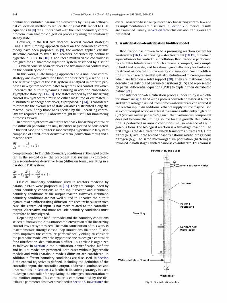

2 nginee

nneps

utshdPo

sTplacdtrlp

tIcr

ctbp

pRbbdcot

sctttfaama3cuttt

first stage is the denitratation which transforms nitrate (NO3) intonitrite (NO2) while the second phase transforms nitrite into gaseousnitrogen (N2). The same micro-organism population (bacteria) isinvolved in both stages, with ethanol as co-substrate. This biomass

44 I. Torres Zúniga et al. / Chemical E

onlinear distributed parameter bioreactors by using an orthogo-al collocation method to reduce the original PDE model to ODEquations. In [8] the authors dealt with the linear boundary controlroblem in an anaerobic digestion process by using the solution atteady state.

However, in the last two decades, several control strategiessing a late lumping approach based on the non-linear controlheory have been proposed. In [9], the authors applied variabletructure control to fixed bed reactors described by nonlinearyperbolic PDEs. In [10] a nonlinear multivariable controller isesigned for an anaerobic digestion system described by a set ofDEs, which consists of an observer and two nonlinear control lawsn the boundary conditions.

In this work, a late lumping approach and a nonlinear controltrategy are investigated for a biofilter described by a set of PDEs.he relative degree of the PDE system is analyzed in order to pro-ose a new system of coordinates to synthesize a control law which

inearizes the output dynamics, assuring in addition closed-loopsymptotic stability [11–13]. The states needed by the linearizingontrol law synthesized must be either measured or estimated. Aistributed Luenberger observer, as proposed in [14], is consideredo estimate the overall set of state variables distributed along theeactor. Even if only those ones needed by the linearizing controlaw are required, this full observer might be useful for monitoringurposes as well.

In order to synthesize an output feedback linearizing controllerhe diffusion phenomenon may be either neglected or considered.n the first case, the biofilter is modeled by a hyperbolic PDE systemomposed of a first-order derivative term (convection term) and aeaction term:

∂�

∂t= −v

∂�

∂z+ r(�)

omplemented by Dirichlet boundary conditions at the input biofil-er. In the second case, the precedent PDE system is completedy a second-order derivative term (diffusion term), resulting in aarabolic PDE system:

∂�

∂t= Df

∂2�

∂z2− v

∂�

∂z+ r(�)

Classical boundary conditions used in reactors modeled byarabolic PDEs were proposed in [15]. They are compounded byobin boundary conditions at the input reactor and Neumannoundary conditions at the output reactor. However, Neumannoundary conditions are not well suited to linearize the outputynamics of biofilters taking diffusion into account because in suchase, the controlled input is not more related to the controlledutput. Alternative and more realistic boundary conditions mustherefore be investigated.

Depending on the biofilter model and the boundary conditionselected, from a simple to a more complete version of the linearizingontrol law are synthesized. The main contribution of this work iso demonstrate, through closed-loop simulations, that the diffusionerm improves the controller performance, yielding to considerhe parabolic model over the hyperbolic one to design a controlleror a nitrification–denitrification biofilter. This article is organizeds follows: in Section 2 the nitrification–denitrification biofilternd its PDE model are presented. Both cases without (hyperbolicodel) and with (parabolic model) diffusion are considered. In

ddition, different boundary conditions are discussed. In Section the control objective is defined, including the definition of theontrolled input, the controlled output, additive disturbances and

ncertainties. In Section 4 a feedback linearizing strategy is usedo design a controller for regulating the nitrogen concentration athe biofilter output. This controller is complemented by the dis-ributed parameter observer developed in Section 5. In Section 6 the

ring Journal 191 (2012) 243– 255

overall observer-based output feedback linearizing control law andits implementation are discussed. In Section 7 numerical resultsare examined. Finally, in Section 8 conclusions about this work arepresented.

2. A nitrification–denitrification biofilter model

Biofiltration has proven to be a promising reaction system forwastewater [16,17] or drinking water treatment [18,19], but also inaquaculture or for control of air pollution. Biofiltration is performedby a biofilter tubular reactor. Such a device is compact, fairly simpleto build and operate, and has shown good efficiency for biologicaltreatment associated to low energy consumption. Such biofiltra-tion unit is characterized by spatial distribution of micro-organismswhich are fixed on a solid support [20]. They are mathematicallydescribed as distributed parameter systems (DPS) and representedby partial differential equations (PDE) to explain their distributednature [21].

The nitrification–denitrification process under study is a biofil-ter, shown in Fig. 1, filled with a porous pouzzolane material. Nitrateand nitrite nitrogen issued from some wastewater are considered atthe reactor input. An additional ethanol supply source may be usedas a control input action or at least to ensure a sufficiently high ratioC/N (carbon source per nitrate) such that carboneous componentdoes not become the limiting source for the growth. Denitrifica-tion is performed in anoxic conditions, i.e., in absence of O2 ingaseous form. The biological reaction is a two-stage reaction. The

Fig. 1. Denitrification biofilter.

nginee

apbetI[n

tocai

N

cf

•

•

•

•

os

S(c(

I. Torres Zúniga et al. / Chemical E

ccumulates on the solid media surface due to filtration of bacteriaresent in the feeding water (if any) and to net growth. Thus, theiomass forms a biofilm around the filter particles, which thick-ns with time. The activity of the part of bacteria not trapped inhe biofilm is negligible with respect to the activity of the biofilm.t is then ignored and one considers that all the biomass is fixed22,19,23]. On the other hand, the soluble compounds (nitrate,itrite and ethanol) are transported along the biofilter.

The objective is to eliminate nitrate and nitrite while goinghrough the biofilter. The bacteria take the organic carbon as sourcef energy. The denitrification metabolic path consists of severalonsecutive oxydoreduction reactions and it implies a transientccumulation of nitrite into the biofilter [24]. It may be dissociatedn two main steps:

O−3

(1)−→NO−2

(2)−→N2

The dynamics of the biofilter can be deduced from mass balanceonsiderations for the four different components, considering theollowing assumptions:

The detachment of biofilm and particles retained by filtration isneglected;Once the biofilm reaches a critical ‘per unit’ surface thickness, thedeeper part of the biofilm is considered as inactivated, and a max-imum active biomass concentration Xamax is reached [19]. Then,after some transition period, the growth of micro-organisms justbalances the death and inactivation process;The decay of biomass is neglected, hidden in the notion of maxi-mum active biomass concentration;Radial dispersion is negligible. Axial dispersion obeys Fick’s dif-fusion law.

The simplest denitrification biofilter model takes into accountnly the convection phenomenon. In this way, it is modeled by aet of hyperbolic partial differential equations (PDE):

∂SNO3 (z, t)

∂t= − v

�∂SNO3 (z, t)

∂z

−1 − Yh1

˛1Yh1�

�1(SNO3 (z, t), SC (z, t))Xa(z, t) (1)

∂SNO2 (z, t)

∂t=− v

�∂SNO2 (z, t)

∂z+ 1 − Yh1

˛1Yh1�

�1(SNO3 (z, t), SC (z, t))Xa(z, t)

− 1 − Yh2

˛2Yh2�

�2(SNO2 (z, t), SC (z, t))Xa(z, t) (2)

∂SC (z, t)∂t

= − v�

∂SC (z, t)∂z

− 1Yh1

��1(SNO3 (z, t), SC (z, t))Xa(z, t)

− 1Yh2

��2(SNO2 (z, t), SC (z, t))Xa(z, t) (3)

∂Xa(z, t)∂t

= (�1(SNO3 (z, t), SC (z, t))Xa(z, t)

+ �2(SNO2 (z, t), SC (z, t))Xa(z, t))(

1 − Xa(z, t)Xamax

)(4)

In the equations above, z is the axial space variable, SNO3 (z, t),

NO2 (z, t), SC(z, t) and Xa(z, t) represent the nitrate (g[N]/m3), nitriteg[N]/m3), ethanol (g[COD]/m3) and active biomass (g[COD]/m3)oncentrations. v, Yh1

, Yh2, �1 and �2 represent the flow rate (m/h)

the ratio between the feeding rate (m3/h) at the reactor input and

ring Journal 191 (2012) 243– 255 245

the biofilter cross-section area (m2)), micro-organisms yield coef-ficients (g/g) and population specific growth rates (g/m3/h) whichtransform nitrate into nitrite, then nitrite into gas nitrogen, respec-tively. Finally, ˛1 and ˛2 are COD conversion coefficients for thenitrate and the nitrite, respectively.

The nitrate and nitrite specific growth rates �1 and �2 dependboth on the microorganism and on environmental parameters ofthe culture like composition, temperature, pH, thermodynamicactivity of the water, standard oxidation–reduction potential, etc.These parameters are however often considered constant and theirinfluence is hidden in the maximum specific growth rates. Thegrowth rates are then typically described by Monod terms, in thisapplication represented as [19]:

�1(SNO3 (z, t), SC (z, t)) = �g�1max

SNO3

SNO3 + KNO3

SC

SC + KC

�2(SNO2 (z, t), SC (z, t)) = �g�2max

SNO2

SNO2 + KNO2

SC

SC + KC

where �g, �1max , �2max , KNO3 , KNO2 and KC are the correction fac-tors for the anaerobic growth, the maximum specific growth ratesof biomass on nitrate and nitrite and the affinity constants withrespect to nitrate, nitrite and ethanol, respectively. However, itmust be pointed out that this model does not always representthe data suitably, especially when the culture media are complexand contain several carbon and nitrogen sources [25].

Associated to the dynamical equations for the denitrificationprocess, appropriate initial spatial profile at t = 0 for 0 ≤ z ≤ Lexpresses that the biomass and the substrate are homogeneouslydistributed along the biofilter:

SNO3 (z, 0) = SNO3,0(z) (5)

SNO2 (z, 0) = SNO2,0(z) (6)

SC (z, 0) = SC,0(z) (7)

Xa(z, 0) = Xa,0(z) (8)

Remark 1. Such an initial profile is considered, without loss ofgenerality, only to simplify the numerical initialization of the sim-ulations. Any other initial profiles could be considered with onlyslight transient differences in the forthcoming simulations, butwithout changing any of the conclusions drawn from the simu-lations.

In addition, hyperbolic PDEs typically consider Dirichlet bound-ary conditions for t > 0 at input:

SNO3 (0, t) = SNO3,in(t) (9)

SNO2 (0, t) = SNO2,in(t) (10)

SC (0, t) = SC,in(t) (11)

where SNO3,in(t), SNO2,in(t) and SC,in(t) represent the nitrate, thenitrite and the ethanol at the biofilter input, respectively.

An extension of the preceding model may be obtained by takinginto account the diffusion phenomenon. In such case, Eqs. (1)–(3)have to be completed on their right sides respectively by a secondorder derivative term of the form:

Df∂2

SNO3 (z, t)

∂z2

Df∂2

SNO2 (z, t)

∂z2

Df∂2

SC (z, t)

∂z2

where Df represents the diffusion term (m2/h).To the best of our knowledge, literature on biofilter model-

ing including diffusion phenomenon has considered Dankwerts

2 nginee

bb

•

•

apfiapccttbttac

•

•

•

46 I. Torres Zúniga et al. / Chemical E

oundary conditions; see [1,26–28] for example. Dankwertsoundary conditions are express as [15]:

Robin boundary conditions for SNO3 , SNO2 and SC at z = 0 (input)for t > 0:

∂SNO3 (0, t)

∂z= v

�Df(SNO3 (0, t) − SNO3,in(t)) (12)

∂SNO2 (0, t)

∂z= v

�Df(SNO2 (0, t) − SNO2,in(t)) (13)

∂SC (0, t)∂z

= v�Df

(SC (0, t) − SC,in(t)) (14)

Neumann boundary conditions at z = L (output) for t > 0:

∂SNO3 (L, t)

∂z= 0 (15)

∂SNO2 (L, t)

∂z= 0 (16)

∂SC (L, t)∂z

= 0 (17)

However, in this article, we would like to discuss those bound-ry conditions. Neumann boundary conditions have been originallyroposed for the heat equation to stress that the temperature pro-le becomes flat at the outlet (in the heat equation, it corresponds ton insulated beam). Even if the diffusion phenomenon which takeslace in the biofilter model assimilates to Fick’s law, such boundaryonditions are not well adapted to the biofilter. Considering that theoncentration is asymptotically constant at the outlet of the biofil-er (or, more exactly, at the limit of the packed material colonized byhe microorganisms) is not physical. This is true only if limitationsy the nutriments occur before the output of the biofilter so thathe reaction rates vanish. Alternatively, dynamic boundary condi-ions, similar to those proposed by Schiesser in [29], would be moreppropriate. This would lead, instead of using Neumann boundaryonditions (15)–(17), to the following alternative options:

Dynamic boundary conditions at z = L (output) for t > 0 with con-vection term:

∂SNO3 (L, t)

∂t= − v

�∂SNO3 (L, t)

∂z(18)

∂SNO2 (L, t)

∂t= − v

�∂SNO2 (L, t)

∂z(19)

∂SC (L, t)∂t

= − v�

∂SC (L, t)∂z

(20)

Dynamic boundary conditions at z = L (output) for t > 0 with dif-fusion and convection terms:

∂SNO3 (L, t)

∂t= Df

∂2SNO3 (L, t)

∂z2− v

�∂SNO3 (L, t)

∂z(21)

∂SNO2 (L, t)

∂t= Df

∂2SNO2 (L, t)

∂z2− v

�∂SNO2 (L, t)

∂z(22)

∂SC (L, t)∂t

= Df∂2

SC (L, t)∂z2

− v�

∂SC (L, t)∂z

(23)

Dynamic boundary conditions at z = L (output) for t > 0 with con-vection and reaction terms:

∂SNO3 (L, t)

∂t= − v

�∂SNO3 (L, t)

∂z

− 1 − Yh1

˛1Yh1�

�1(SNO3 (L, t), SC (L, t))Xa(L, t) (24)

ring Journal 191 (2012) 243– 255

∂SNO2 (L, t)

∂t= − v

�∂SNO2 (L, t)

∂z

+1 − Yh1

˛1Yh1�

�1(SNO3 (L, t), SC (L, t))Xa(L, t)

− 1 − Yh2

˛2Yh2�

�2(SNO2 (L, t), SC (L, t))Xa(L, t) (25)

∂SC (L, t)∂t

= − v�

∂SC (L, t)∂z

− 1Yh1

��1(SNO3 (L, t), SC (L, t))Xa(L, t)

− 1Yh2

��2(SNO2 (L, t), SC (L, t))Xa(L, t) (26)

• Dynamic boundary conditions at z = L (output) for t > 0 with dif-fusion, convection and reaction terms:

∂SNO3 (L, t)

∂t= Df

∂2SNO3 (L, t)

∂z2− v

�∂SNO3 (L, t)

∂z

− 1 − Yh1

˛1Yh1�

�1(SNO3 (L, t), SC (L, t))Xa(L, t) (27)

∂SNO2 (L, t)

∂t= Df

∂2SNO2 (L, t)

∂z2− v

�∂SNO2 (L, t)

∂z

+ 1 − Yh1

˛1Yh1�

�1(SNO3 (L, t), SC (L, t))Xa(L, t)

−1 − Yh2

˛2Yh2�

�2(SNO2 (L, t), SC (L, t))Xa(L, t) (28)

∂SC (L, t)∂t

= Df∂2

SC (L, t)∂z2

− v�

∂SC (L, t)∂z

− 1Yh1

��1(SNO3 (L, t), SC (L, t))Xa(L, t)

− 1Yh2

��2(SNO2 (L, t), SC (L, t))Xa(L, t) (29)

Remark 2. Such dynamic boundary conditions express whichphenomena are present at the biofilter outlet. In the first case, con-vection dominates as expressed by Neumann boundary conditions.In the second case only diffusion and convection are present indi-cating that no reaction occurs at the reactor output. In the thirdcase, the diffusion phenomenon is neglected. Finally, in the fourthcase all phenomena are taken into account.

Further, one could also conceive of transforming such two-pointboundary-value problems into a single-point boundary conditionproblem, where space boundary conditions are all set at the inputof the biofilter. Historically, classical boundary conditions havebeen proposed at the two end points to evaluate analytical solu-tions of PDEs problems. Even if the resulting problem is no longerHadamard-correctly posed [30], it is legitimate to consider Dirichletboundary conditions associated to the Robin boundary conditionsdescribed above.

Remark 3. The idea behind the terminology of Hadamard-correctly posed stresses that the Cauchy problem (existence andunicity of a solution to a PDEs problem) may be weakened, espe-

cially from a numerical simulation point of view [30]. Actually, thewave equation problem in two variables with boundary conditionsall set at the same point is correctly posed in the sense of Hadamard[30]. Moreover, it has been recently shown that, using ideas issued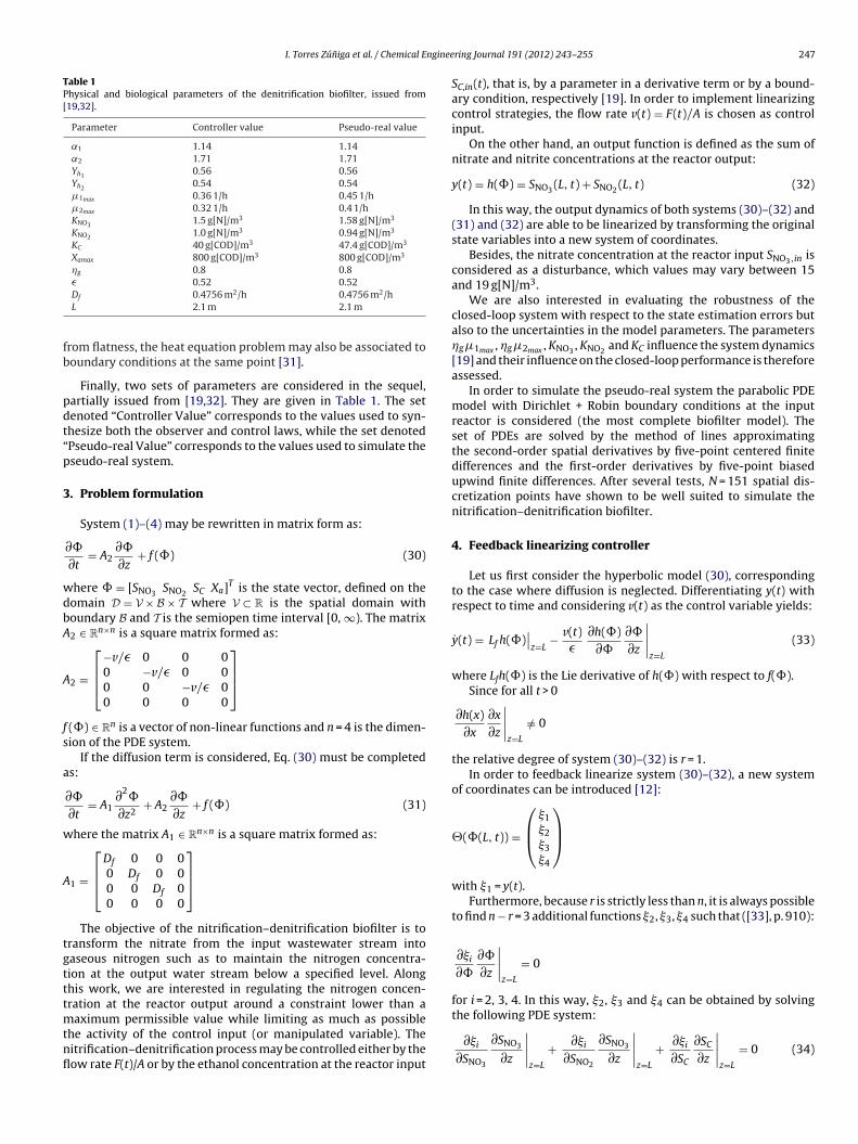

I. Torres Zúniga et al. / Chemical Enginee

Table 1Physical and biological parameters of the denitrification biofilter, issued from[19,32].

Parameter Controller value Pseudo-real value

˛1 1.14 1.14˛2 1.71 1.71Yh1

0.56 0.56Yh2

0.54 0.54�1max 0.36 1/h 0.45 1/h�2max 0.32 1/h 0.4 1/hKNO3 1.5 g[N]/m3 1.58 g[N]/m3

KNO2 1.0 g[N]/m3 0.94 g[N]/m3

KC 40 g[COD]/m3 47.4 g[COD]/m3

Xamax 800 g[COD]/m3 800 g[COD]/m3

�g 0.8 0.8� 0.52 0.52

fb

pdt“p

3

wdbA

A

fs

a

w

A

tgtttmtnfl

Df 0.4756 m2/h 0.4756 m2/hL 2.1 m 2.1 m

rom flatness, the heat equation problem may also be associated tooundary conditions at the same point [31].

Finally, two sets of parameters are considered in the sequel,artially issued from [19,32]. They are given in Table 1. The setenoted “Controller Value” corresponds to the values used to syn-hesize both the observer and control laws, while the set denotedPseudo-real Value” corresponds to the values used to simulate theseudo-real system.

. Problem formulation

System (1)–(4) may be rewritten in matrix form as:

∂�

∂t= A2

∂�

∂z+ f (�) (30)

here � = [SNO3 SNO2 SC Xa]T is the state vector, defined on theomain D = V × B × T where V ⊂ R is the spatial domain withoundary B and T is the semiopen time interval [0, ∞). The matrix2 ∈ R

n×n is a square matrix formed as:

2 =

⎡⎢⎣

−v/� 0 0 00 −v/� 0 00 0 −v/� 00 0 0 0

⎤⎥⎦

(�) ∈ Rn is a vector of non-linear functions and n = 4 is the dimen-

ion of the PDE system.If the diffusion term is considered, Eq. (30) must be completed

s:

∂�

∂t= A1

∂2�

∂z2+ A2

∂�

∂z+ f (�) (31)

here the matrix A1 ∈ Rn×n is a square matrix formed as:

1 =

⎡⎢⎣

Df 0 0 00 Df 0 00 0 Df 00 0 0 0

⎤⎥⎦

The objective of the nitrification–denitrification biofilter is toransform the nitrate from the input wastewater stream intoaseous nitrogen such as to maintain the nitrogen concentra-ion at the output water stream below a specified level. Alonghis work, we are interested in regulating the nitrogen concen-ration at the reactor output around a constraint lower than a

aximum permissible value while limiting as much as possiblehe activity of the control input (or manipulated variable). Theitrification–denitrification process may be controlled either by theow rate F(t)/A or by the ethanol concentration at the reactor input

ring Journal 191 (2012) 243– 255 247

SC,in(t), that is, by a parameter in a derivative term or by a bound-ary condition, respectively [19]. In order to implement linearizingcontrol strategies, the flow rate v(t) = F(t)/A is chosen as controlinput.

On the other hand, an output function is defined as the sum ofnitrate and nitrite concentrations at the reactor output:

y(t) = h(�) = SNO3 (L, t) + SNO2 (L, t) (32)

In this way, the output dynamics of both systems (30)–(32) and(31) and (32) are able to be linearized by transforming the originalstate variables into a new system of coordinates.

Besides, the nitrate concentration at the reactor input SNO3,in isconsidered as a disturbance, which values may vary between 15and 19 g[N]/m3.

We are also interested in evaluating the robustness of theclosed-loop system with respect to the state estimation errors butalso to the uncertainties in the model parameters. The parameters�g�1max , �g�2max , KNO3 , KNO2 and KC influence the system dynamics[19] and their influence on the closed-loop performance is thereforeassessed.

In order to simulate the pseudo-real system the parabolic PDEmodel with Dirichlet + Robin boundary conditions at the inputreactor is considered (the most complete biofilter model). Theset of PDEs are solved by the method of lines approximatingthe second-order spatial derivatives by five-point centered finitedifferences and the first-order derivatives by five-point biasedupwind finite differences. After several tests, N = 151 spatial dis-cretization points have shown to be well suited to simulate thenitrification–denitrification biofilter.

4. Feedback linearizing controller

Let us first consider the hyperbolic model (30), correspondingto the case where diffusion is neglected. Differentiating y(t) withrespect to time and considering v(t) as the control variable yields:

y(t) = Lf h(�)∣∣z=L

− v(t)�

∂h(�)∂�

∂�

∂z

∣∣∣∣z=L

(33)

where Lfh(�) is the Lie derivative of h(�) with respect to f(�).Since for all t > 0

∂h(x)∂x

∂x

∂z

∣∣∣∣z=L

/= 0

the relative degree of system (30)–(32) is r = 1.In order to feedback linearize system (30)–(32), a new system

of coordinates can be introduced [12]:

�(�(L, t)) =

⎛⎜⎝

�1�2�3�4

⎞⎟⎠

with �1 = y(t).Furthermore, because r is strictly less than n, it is always possible

to find n − r = 3 additional functions �2, �3, �4 such that ([33], p. 910):

∂�i

∂�

∂�

∂z

∣∣∣∣z=L

= 0

for i = 2, 3, 4. In this way, �2, �3 and �4 can be obtained by solving

the following PDE system:

∂�i

∂SNO3

∂SNO3

∂z

∣∣∣∣z=L

+ ∂�i

∂SNO2

∂SNO3

∂z

∣∣∣∣z=L

+ ∂�i

∂SC

∂SC

∂z

∣∣∣∣z=L

= 0 (34)

2 nginee

te

t

o

wc

t

ccoAm

v

w

pe(

y

bs

ic

y

48 I. Torres Zúniga et al. / Chemical E

It must be pointed out that solving the PDE system above is aedious task because it depends on the solution of the original statequations.

According to (33) and denoting:

a(�) = Lf h(�)∣∣z=L

b(�) = −1�

∂h(�)∂�

∂�

∂z

∣∣∣∣z=L

he following representation is obtained:

d�1

dt= ∂�1

∂�

∂�

∂t= a(�) + b(�)v(t) (35)

Because �2, �3 and �4 have been chosen so that

∂�i

∂�

∂�

∂z

∣∣∣∣z=L

= 0

ne has for i = 2, 3, 4,

d�i

dt= ∂�i

∂�

(f (�) − v(t)

�∂�

∂z

)∣∣∣∣z=L

= Lf �i

∣∣z=L

− v(t)�

∂�i

∂�

∂�

∂z

∣∣∣∣z=L

= Lf �i

∣∣z=L

= qi(�) (36)

here the first derivative with respect to z of the vector � fourthomponent (Xa) is zero.

The state space description of the original system (30)–(32) inhe new coordinates can then be written as:

�1 = a(�) + b(�)v(t)�2 = q2(�)�3 = q3(�)�4 = q4(�)

(37)

The objective is to build a control law v(t) which stabilizes thelosed-loop system and such that the output y(t) tracks a givenonstant reference yr while limiting as much as possible the activityf the control input. Let us define the tracking error e0 as y(t) − yr.s soon as the original system (30)–(32) is locally exponentiallyinimum phase and ˛0 > 0, the following control law:

(t) = 1b(�)

(−a(�) − ˛0e0

)(38)

ith:

a(�) = −1 − Yh2

˛2Yh2�

�2(SNO2 , SC )Xa

∣∣∣∣z=L

b(�) = −1�

(∂SNO3

∂z+ ∂SNO2

∂z

)∣∣∣∣z=L

e0 =(

SNO3 + SNO2 − yr

)∣∣z=L

(39)

artially linearizes the original system and results in a (locally)xponentially stable closed-loop system [13]. Thus, by inspecting37) the resulting closed-loop dynamics are given by:

˙ (t) = −˛0 (y(t) − yr) (40)

ecause it is sufficient to differentiate once the output function toee explicitly the control input.

If the diffusion phenomenon is taken into account, model (31)s considered. Then, differentiating y(t) with respect to time and

onsidering v(t) as the control variable yields:

˙ (t) = Df∂h(�)

∂�

∂2�

∂z2

∣∣∣∣z=L

+ Lf h(�)∣∣z=L

− v(t)�

∂h(�)∂�

∂�

∂z

∣∣∣∣z=L

(41)

ring Journal 191 (2012) 243– 255

As soon as Neumann boundary conditions are not considered atthe biofilter output, one has, for all t > 0:

∂h(�)∂�

∂�

∂z

∣∣∣∣z=L

/= 0

According to the discussion about boundary conditions ofparabolic PDEs in Section 2, five cases may be considered. First,if Robin boundary conditions are considered at the biofilter inputand Dynamic boundary conditions (18)–(20) are considered at thebiofilter output, the control law (38) is synthesized with:

a(�) = 0

b(�) = −1�

(∂SNO3

∂z+ ∂SNO2

∂z

)∣∣∣∣z=L

e0 = (SNO3 + SNO2 − yr)∣∣z=L

(42)

If dynamic boundary conditions (21)–(23) are considered at thebiofilter output, the control law (38) is synthesized with:

a(�) =(

Df∂2

SNO3

∂z2+ Df

∂2SNO2

∂z2

)∣∣∣∣∣z=L

b(�) = −1�

(∂SNO3

∂z+ ∂SNO2

∂z

)∣∣∣∣z=L

e0 =(

SNO3 + SNO2 − yr

)∣∣z=L

(43)

If dynamic boundary conditions (24)–(26) are considered at thebiofilter output, the control law (38) is synthesized with a(�), b(�)and e0 as in the hyperbolic-model based case.

On the other hand, if either, dynamic boundary conditions(27)–(29) are considered at the biofilter output or a combination ofDirichlet + Robin boundary conditions are considered at the biofil-ter input, the control law (38) is synthesized with:

a(�) =(

Df

∂2SNO3

∂z2+ Df

∂2SNO2

∂z2− 1 − Yh2

˛2Yh2�

�2(SNO2 , SC )Xa

)∣∣∣∣z=L

b(�) = −1�

(∂SNO3

∂z+ ∂SNO2

∂z

)∣∣∣z=L

e0 =(

SNO3 + SNO2 − yr

)∣∣z=L

(44)

In all cases, the value of ˛0 has to be sufficiently small to rejectthe influence of the SNO3 and SNO2 derivatives at the reactor out-put in the output dynamics but large enough to bypass the modeluncertainties, especially those that come from �2(SNO2 , SC ) in thefirst and third cases.

5. Distributed parameter observer

In order to implement the control law (38), with (39), (42), (43)or (44) it is necessary to know the nitrite and ethanol concentra-tions to compute �2(SNO2 , SC ), the biomass concentration and thespatial derivatives of both the nitrate and the nitrite concentrations,at the reactor output. An observer is therefore selected to estimatethe non-available concentrations. Since DPS dynamics are charac-terized by an infinite number of modes, the design of an observerwould in principle require the specification of a large (theoreti-cally infinite) number of tuning parameters. In order to bypassthis high-dimensional design problem, a late lumping approach

to the construction of distributed parameter observers (DPO) wasdeveloped in [14]. A nonlinear distributed parameter observer(DPO), with a formulation analog to the Luenberger observer, isthen designed so as to assign the error dynamics to estimate the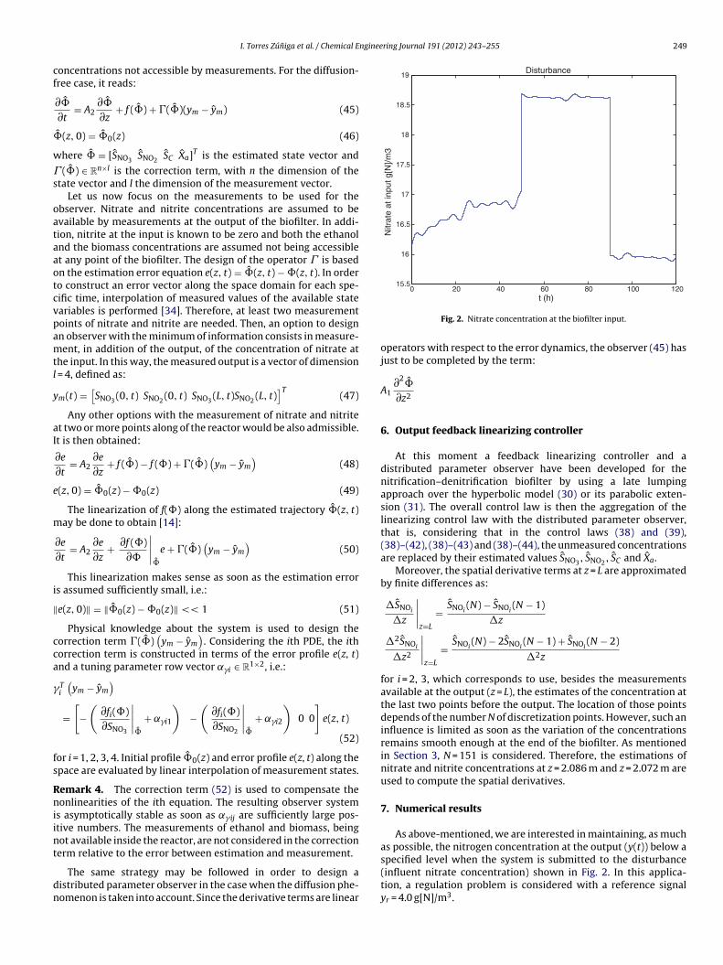

ngineering Journal 191 (2012) 243– 255 249

cf

�

w

s

oataaotcvpamtl

y

aI

e

m

i

‖

cca

�

fs

Rniint

dn

0 20 40 60 80 100 12015.5

16

16.5

17

17.5

18

18.5

19

Nitr

ate

at in

put g

[N]/m

3

Disturbance

I. Torres Zúniga et al. / Chemical E

oncentrations not accessible by measurements. For the diffusion-ree case, it reads:

∂�

∂t= A2

∂�

∂z+ f (�) + (�)(ym − ym) (45)

ˆ (z, 0) = �0(z) (46)

here � = [SNO3 SNO2 SC Xa]T is the estimated state vector and

(�) ∈ Rn×l is the correction term, with n the dimension of the

tate vector and l the dimension of the measurement vector.Let us now focus on the measurements to be used for the

bserver. Nitrate and nitrite concentrations are assumed to bevailable by measurements at the output of the biofilter. In addi-ion, nitrite at the input is known to be zero and both the ethanolnd the biomass concentrations are assumed not being accessiblet any point of the biofilter. The design of the operator is basedn the estimation error equation e(z, t) = �(z, t) − �(z, t). In ordero construct an error vector along the space domain for each spe-ific time, interpolation of measured values of the available stateariables is performed [34]. Therefore, at least two measurementoints of nitrate and nitrite are needed. Then, an option to designn observer with the minimum of information consists in measure-ent, in addition of the output, of the concentration of nitrate at

he input. In this way, the measured output is a vector of dimension = 4, defined as:

m(t) =[SNO3 (0, t) SNO2 (0, t) SNO3 (L, t)SNO2 (L, t)

]T(47)

Any other options with the measurement of nitrate and nitritet two or more points along of the reactor would be also admissible.t is then obtained:

∂e

∂t= A2

∂e

∂z+ f (�) − f (�) + (�)

(ym − ym

)(48)

(z, 0) = �0(z) − �0(z) (49)

The linearization of f(�) along the estimated trajectory �(z, t)ay be done to obtain [14]:

∂e

∂t= A2

∂e

∂z+ ∂f (�)

∂�

∣∣∣∣�

e + (�)(

ym − ym

)(50)

This linearization makes sense as soon as the estimation errors assumed sufficiently small, i.e.:

e(z, 0)‖ = ‖�0(z) − �0(z)‖ << 1 (51)

Physical knowledge about the system is used to design theorrection term (�)

(ym − ym

). Considering the ith PDE, the ith

orrection term is constructed in terms of the error profile e(z, t)nd a tuning parameter row vector ˛�i ∈ R

1×2, i.e.:

Ti

(ym − ym

)=[−(

∂fi(�)∂SNO3

∣∣∣∣�

+ ˛�i1

)−(

∂fi(�)∂SNO2

∣∣∣∣�

+ ˛�i2

)0 0

]e(z, t)

(52)

or i = 1, 2, 3, 4. Initial profile �0(z) and error profile e(z, t) along thepace are evaluated by linear interpolation of measurement states.

emark 4. The correction term (52) is used to compensate theonlinearities of the ith equation. The resulting observer system

s asymptotically stable as soon as ˛� ij are sufficiently large pos-tive numbers. The measurements of ethanol and biomass, beingot available inside the reactor, are not considered in the correction

erm relative to the error between estimation and measurement.

The same strategy may be followed in order to design aistributed parameter observer in the case when the diffusion phe-omenon is taken into account. Since the derivative terms are linear

t (h)

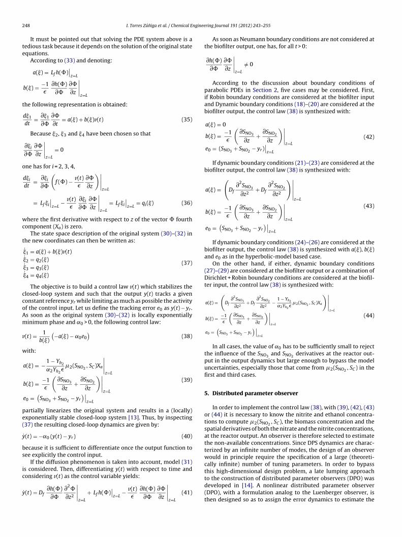
Fig. 2. Nitrate concentration at the biofilter input.

operators with respect to the error dynamics, the observer (45) hasjust to be completed by the term:

A1∂2

�

∂z2

6. Output feedback linearizing controller

At this moment a feedback linearizing controller and adistributed parameter observer have been developed for thenitrification–denitrification biofilter by using a late lumpingapproach over the hyperbolic model (30) or its parabolic exten-sion (31). The overall control law is then the aggregation of thelinearizing control law with the distributed parameter observer,that is, considering that in the control laws (38) and (39),(38)–(42), (38)–(43) and (38)–(44), the unmeasured concentrationsare replaced by their estimated values SNO3 , SNO2 , SC and Xa.

Moreover, the spatial derivative terms at z = L are approximatedby finite differences as:

�SNOi

�z

∣∣∣∣z=L

= SNOi(N) − SNOi

(N − 1)

�z

�2SNOi

�z2

∣∣∣∣z=L

= SNOi(N) − 2SNOi

(N − 1) + SNOi(N − 2)

�2z

for i = 2, 3, which corresponds to use, besides the measurementsavailable at the output (z = L), the estimates of the concentration atthe last two points before the output. The location of those pointsdepends of the number N of discretization points. However, such aninfluence is limited as soon as the variation of the concentrationsremains smooth enough at the end of the biofilter. As mentionedin Section 3, N = 151 is considered. Therefore, the estimations ofnitrate and nitrite concentrations at z = 2.086 m and z = 2.072 m areused to compute the spatial derivatives.

7. Numerical results

As above-mentioned, we are interested in maintaining, as muchas possible, the nitrogen concentration at the output (y(t)) below a

specified level when the system is submitted to the disturbance(influent nitrate concentration) shown in Fig. 2. In this applica-tion, a regulation problem is considered with a reference signalyr = 4.0 g[N]/m3.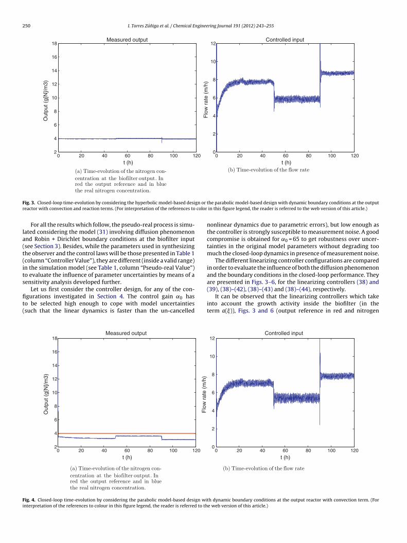

250 I. Torres Zúniga et al. / Chemical Engineering Journal 191 (2012) 243– 255

0 20 40 60 80 100 1202

4

6

8

10

12

14

16

18

t (h)

Out

put (

g[N

]/m3)

Measured output

0 20 40 60 80 100 1200

2

4

6

8

10

12

t (h)

Flo

w r

ate

(m/h

)

Controlled input

(a) Ti me-evolu tion of the ni trog en con- (b) Ti me-evolu tion of the flow ��������� � � � � � � � � � � � � � � � � � � � � � � � � � � � � � � � � � � � �ratecentration at the biofilter�� � � � � � � � � �output���� � � � � �.��� � � � � � � � � � � � � � � � � � � � � � � � � � � � � � � � � � � � � � � � � � � � � � � � � � � � � �Inred the outpu t reference and in bluethe real ni trog en conce ntration.

F gn or

r color

la(t(its

fit(

Fi

ig. 3. Closed-loop time-evolution by considering the hyperbolic model-based desieactor with convection and reaction terms. (For interpretation of the references to

For all the results which follow, the pseudo-real process is simu-ated considering the model (31) involving diffusion phenomenonnd Robin + Dirichlet boundary conditions at the biofilter inputsee Section 3). Besides, while the parameters used in synthesizinghe observer and the control laws will be those presented in Table 1column “Controller Value”), they are different (inside a valid range)n the simulation model (see Table 1, column “Pseudo-real Value”)o evaluate the influence of parameter uncertainties by means of aensitivity analysis developed further.

Let us first consider the controller design, for any of the con-

gurations investigated in Section 4. The control gain ˛0 haso be selected high enough to cope with model uncertaintiessuch that the linear dynamics is faster than the un-cancelled

0 20 40 60 80 100 1202

4

6

8

10

12

14

16

18

t (h)

Out

put (

g[N

]/m3)

Measured output

Flo

w r

ate

(m/h

)

(a) Ti me-evolu tion of the ni trog en con- centration at the biofilter�� � � � � � � � � �output���� � � � � �.��� � � � � � � � � � � � � � � � � � � � � � � � � � � � � � � � � � � � � � � � � � � � � � � � � � � � � �Inred the outpu t reference and in bluethe real ni trog en conce ntration.

ig. 4. Closed-loop time-evolution by considering the parabolic model-based design winterpretation of the references to colour in this figure legend, the reader is referred to th

the parabolic model-based design with dynamic boundary conditions at the output in this figure legend, the reader is referred to the web version of this article.)

nonlinear dynamics due to parametric errors), but low enough asthe controller is strongly susceptible to measurement noise. A goodcompromise is obtained for ˛0 = 65 to get robustness over uncer-tainties in the original model parameters without degrading toomuch the closed-loop dynamics in presence of measurement noise.

The different linearizing controller configurations are comparedin order to evaluate the influence of both the diffusion phenomenonand the boundary conditions in the closed-loop performance. Theyare presented in Figs. 3–6, for the linearizing controllers (38) and(39), (38)–(42), (38)–(43) and (38)–(44), respectively.

It can be observed that the linearizing controllers which takeinto account the growth activity inside the biofilter (in theterm a(�)), Figs. 3 and 6 (output reference in red and nitrogen

0 20 40 60 80 100 1200

2

4

6

8

10

12

t (h)

Controlled input

(b) Ti me-evolu tion of the flow ��������� � � � � � � � � � � � � � � � � � � � � � � � � � � � � � � � � � � � �rate

th dynamic boundary conditions at the output reactor with convection term. (Fore web version of this article.)

I. Torres Zúniga et al. / Chemical Engineering Journal 191 (2012) 243– 255 251

0 20 40 60 80 100 1202

4

6

8

10

12

14

16

18

t (h)

Out

put (

g[N

]/m3)

Measured output

0 20 40 60 80 100 1200

2

4

6

8

10

12

t (h)

Flo

w r

ate

(m/h

)

Controlled input

(a) Ti me-evolu tion of the ni trog en con- (b) Ti me-evolu tion of the flow ��������� � � � � � � � � � � � � � � � � � � � � � � � � � � � � � � � � � � � �ratecentration at the biofilter�� � � � � � � � � �output���� � � � � �.��� � � � � � � � � � � � � � � � � � � � � � � � � � � � � � � � � � � � � � � � � � � � � � � � � � � � � �Inred the outpu t reference and in bluethe real ni trog en conce ntration.

F n witht r is re

cece1

taulmct

Fct

ig. 5. Closed-loop time-evolution by considering the parabolic model-based desigerms. (For interpretation of the references to colour in this figure legend, the reade

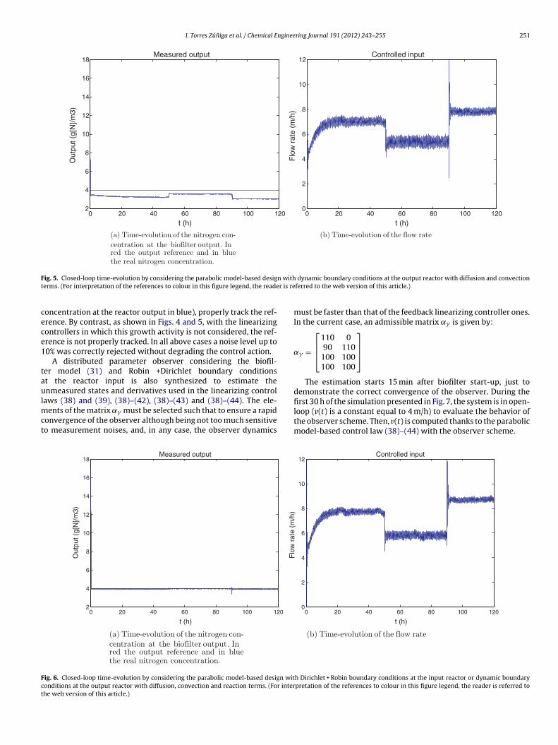
oncentration at the reactor output in blue), properly track the ref-rence. By contrast, as shown in Figs. 4 and 5, with the linearizingontrollers in which this growth activity is not considered, the ref-rence is not properly tracked. In all above cases a noise level up to0% was correctly rejected without degrading the control action.

A distributed parameter observer considering the biofil-er model (31) and Robin +Dirichlet boundary conditionst the reactor input is also synthesized to estimate thenmeasured states and derivatives used in the linearizing control

aws (38) and (39), (38)–(42), (38)–(43) and (38)–(44). The ele-ents of the matrix ˛� must be selected such that to ensure a rapid

onvergence of the observer although being not too much sensitiveo measurement noises, and, in any case, the observer dynamics

0 20 40 60 80 100 1202

4

6

8

10

12

14

16

18

t (h)

Out

put (

g[N

]/m3)

Measured output

(a) Ti me-evolu tion of the ni trog en con- centration at the biofilter�� � � � � � � � � �output���� � � � � �.��� � � � � � � � � � � � � � � � � � � � � � � � � � � � � � � � � � � � � � � � � � � � � � � � � � � � � �Inred the outpu t reference and in bluethe real ni trog en conce ntration.

ig. 6. Closed-loop time-evolution by considering the parabolic model-based design witonditions at the output reactor with diffusion, convection and reaction terms. (For interhe web version of this article.)

dynamic boundary conditions at the output reactor with diffusion and convectionferred to the web version of this article.)

must be faster than that of the feedback linearizing controller ones.In the current case, an admissible matrix ˛� is given by:

˛� =

⎡⎢⎣

110 090 110

100 100100 100

⎤⎥⎦

The estimation starts 15 min after biofilter start-up, just todemonstrate the correct convergence of the observer. During the

first 30 h of the simulation presented in Fig. 7, the system is in open-loop (v(t) is a constant equal to 4 m/h) to evaluate the behavior ofthe observer scheme. Then, v(t) is computed thanks to the parabolicmodel-based control law (38)–(44) with the observer scheme.

0 20 40 60 80 100 1200

2

4

6

8

10

12

t (h)

Flo

w r

ate

(m/h

)

Controlled input

(b) Ti me-evolu tion of the flow ��������� � � � � � � � � � � � � � � � � � � � � � � � � � � � � � � � � � � � �rate

h Dirichlet + Robin boundary conditions at the input reactor or dynamic boundarypretation of the references to colour in this figure legend, the reader is referred to

252 I. Torres Zúniga et al. / Chemical Engineering Journal 191 (2012) 243– 255

0 20 40 60 80 100 120−9

−8

−7

−6

−5

−4

−3

−2

−1

0

1

t (h)

Nitr

ate

first

der

ivat

ive

NO3 first derivative at the reactor output

(a) NO3 derivative at z = L.

0 20 40 60 80 100 120−6

−5

−4

−3

−2

−1

0

1

2

t (h)

Nitr

ite fi

rst d

eriv

ativ

e

NO2 first derivative at the reactor output

(b) NO2 derivative at z = L.

0 20 40 60 80 100 120−2

0

2

4

6

8

10

12

14

16

t (h)

Nitr

ate

seco

nd d

eriv

ativ

e

NO3 second derivative at the reactor output

(c) NO3 sec ond derivative at z = L.

0 20 40 60 80 100 120−15

−10

−5

0

5

10

t (h)

Nitr

ite s

econ

d de

rivat

ive

NO2 second derivative at the reactor output

(d) NO2 sec ond derivative at z = L.

0 20 40 60 80 100 1200

20

40

60

80

100

120

t (h)

Eth

anol

g[C

OD

]/m3

SC concentration at the reactor output

(e) SC conce ntration at z = L.

0 20 40 60 80 100 1200

100

200

300

400

500

600

700

800

900

t (h)

Bio

mas

s g[

CO

D]/m

3

Xa concentration at the reactor output

(f) Xa conce ntration at z = L.

F es fori to th

rfifiSa

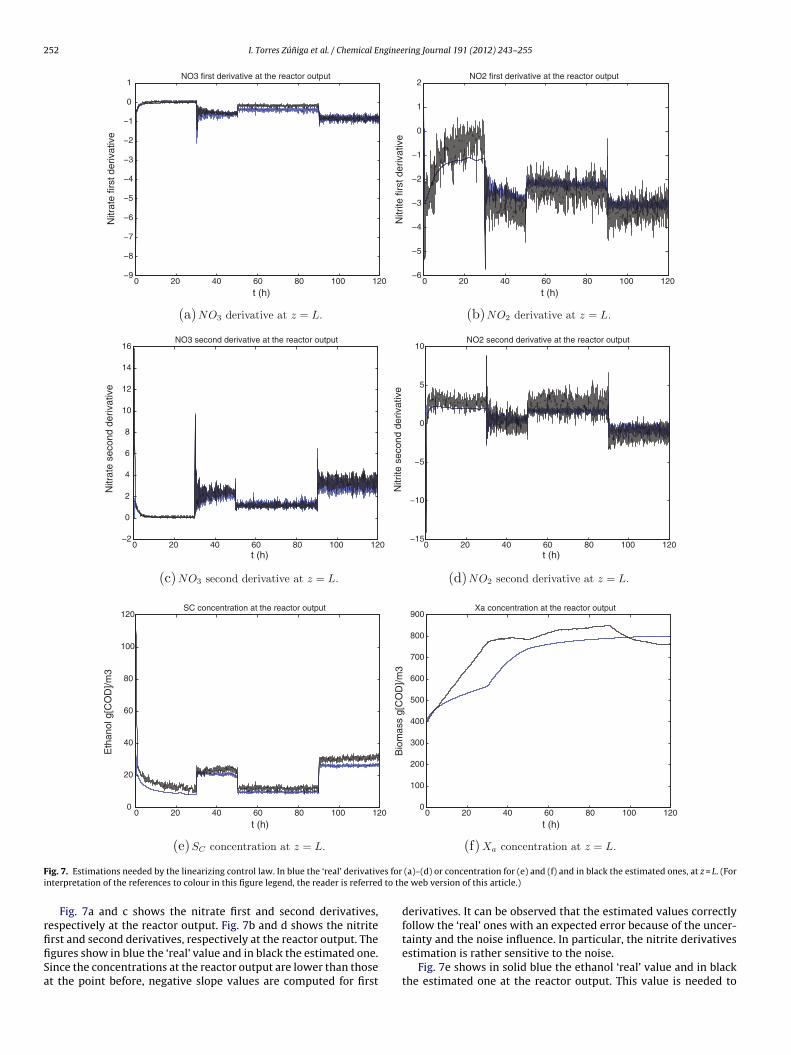
ig. 7. Estimations needed by the linearizing control law. In blue the ‘real’ derivativnterpretation of the references to colour in this figure legend, the reader is referred

Fig. 7a and c shows the nitrate first and second derivatives,espectively at the reactor output. Fig. 7b and d shows the nitrite

rst and second derivatives, respectively at the reactor output. Thegures show in blue the ‘real’ value and in black the estimated one.ince the concentrations at the reactor output are lower than thoset the point before, negative slope values are computed for first

(a)–(d) or concentration for (e) and (f) and in black the estimated ones, at z = L. (Fore web version of this article.)

derivatives. It can be observed that the estimated values correctlyfollow the ‘real’ ones with an expected error because of the uncer-

tainty and the noise influence. In particular, the nitrite derivativesestimation is rather sensitive to the noise.

Fig. 7e shows in solid blue the ethanol ‘real’ value and in blackthe estimated one at the reactor output. This value is needed to

I. Torres Zúniga et al. / Chemical Engineering Journal 191 (2012) 243– 255 253

0 20 40 60 80 100 1200

2

4

6

8

10

12

14

16

18

t (h)

Out

put (

g[N

]/m3)

Measured output

0 20 40 60 80 100 1200

2

4

6

8

10

12

t (h)

Flo

w r

ate

(m/h

)

Controlled input

(a) Ti me-evolu tion of the ni trog en con- (b) Ti me-evolu tion of the flow ��������� � � � � � � � � � � � � � � � � � � � � � � � � � � � � � � � � � � � �rate

centration at the biofilter�� � � � � � � � � �output���� � � � � �.��� � � � � � � � � � � � � � � � � � � � � � � � � � � � � � � � � � � � � � � � � � � � � � � � � � � � � �In

red the outpu t reference and in blue

the real ni trog en conce ntration.

F e hypc

cb

t41a

(oTop

F(r

ig. 8. Closed-loop time-evolution by considering the observer-based version of tholour in this figure legend, the reader is referred to the web version of this article.)

ompute the growth term �2(SNO2 , SC ) at the reactor output. Theias in the estimation is related to the model uncertainties.

Fig. 7f shows in solid blue the biomass ‘real’ value and in blackhe estimated one at the reactor output. The initial biomass is set to00 g[COD]/m3 and approximately reaches its maximal value after00 h. A poor estimation is observed because of the uncertaintiesnd the lack of measurements.

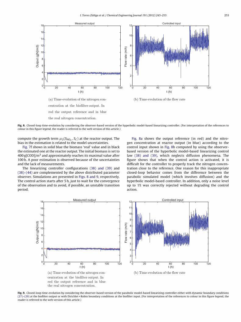
The linearizing controller configurations (38) and (39) and38)–(44) are complemented by the above distributed parameter

bserver. Simulations are presented in Figs. 8 and 9, respectively.he control action starts after 5 h, just to wait for the convergencef the observation and to avoid, if possible, an unstable transitioneriod.

0 20 40 60 80 100 1200

2

4

6

8

10

12

14

16

18

t (h)

Out

put (

g[N

]/m3)

Measured output

(a) Ti me-evolu tion of the ni trog en con- centration at the biofilter���� � � � � � � � � � � � � � � � � � � � � � � � � � � � � � � � � � � �output���.��� � � � � � � � � � � � � � � � � � � � � � � � � � � � � � � � � � � � � � � � � � � � � � � � � � � � � � �Inred the outpu t reference and in bluethe real ni trog en conce ntration.

ig. 9. Closed-loop time-evolution by considering the observer-based version of the para27)–(29) at the biofilter output or with Dirichlet + Robin boundary conditions at the biofieader is referred to the web version of this article.)

erbolic model-based linearizing controller. (For interpretation of the references to

Fig. 8a shows the output reference (in red) and the nitro-gen concentration at reactor output (in blue) according to thecontrol input shown in Fig. 8b computed by using the observer-based version of the hyperbolic model-based linearizing controllaw (38) and (39), which neglects diffusion phenomena. Thefigure shows that when the control action is activated, it isdifficult for the controller to properly track the nitrogen concen-tration close to the reference. One reason for this inappropriateclosed-loop behavior comes from the difference between the

parabolic simulated model (which involves diffusion) and thehyperbolic model-based controller. In addition, only a noise levelup to 1% was correctly rejected without degrading the controlaction.

0 20 40 60 80 100 1202

3

4

5

6

7

8

9

10

11

12

t (h)

Flo

w r

ate

(m/h

)

Controlled input

(b) Ti me-evolu tion of the flo w rate

bolic model-based linearizing controller either with dynamic boundary conditionslter input. (For interpretation of the references to colour in this figure legend, the

2 ngineering Journal 191 (2012) 243– 255

b(rpee2a

pe(blh

cltisecpfp

pttfcim

y

tpSty

P

H−dyee

mvuta

RvIbsc

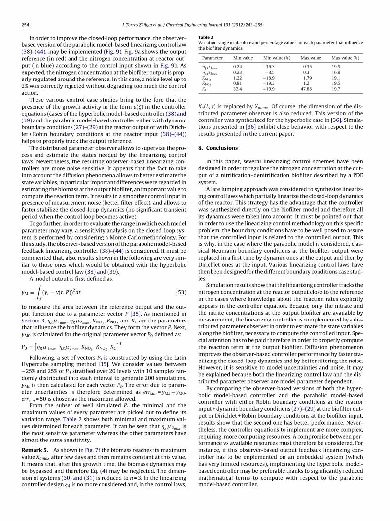
Table 2Variation range in absolute and percentage values for each parameter that influencethe biofilter dynamics.

Parameter Min value Min value (%) Max value Max value (%)

�g�1max 0.24 −16.3 0.35 19.9�g�2max 0.23 −8.5 0.3 16.9

54 I. Torres Zúniga et al. / Chemical E

In order to improve the closed-loop performance, the observer-ased version of the parabolic model-based linearizing control law38)–(44), may be implemented (Fig. 9). Fig. 9a shows the outputeference (in red) and the nitrogen concentration at reactor out-ut (in blue) according to the control input shown in Fig. 9b. Asxpected, the nitrogen concentration at the biofilter output is prop-rly regulated around the reference. In this case, a noise level up to% was correctly rejected without degrading too much the controlction.

These various control case studies bring to the fore that theresence of the growth activity in the term a(�) in the controllerquations (cases of the hyperbolic model-based controller (38) and39) and the parabolic model-based controller either with dynamicoundary conditions (27)–(29) at the reactor output or with Dirich-

et + Robin boundary conditions at the reactor input (38)–(44))elps to properly track the output reference.

The distributed parameter observer allows to supervize the pro-ess and estimate the states needed by the linearizing controlaws. Nevertheless, the resulting observer-based linearizing con-rollers are more noise sensitive. It appears that the fact to takento account the diffusion phenomena allows to better estimate thetate variables, in particular important differences were regarded instimating the biomass at the output biofilter, an important value toompute the reaction term. It results in a smoother control input inresence of measurement noise (better filter effect), and allows toaster stabilize the closed-loop dynamics (no significant transienteriod when the control loop becomes active).

To go further, in order to evaluate the range in which each modelarameter may vary, a sensitivity analysis on the closed-loop sys-em is performed by considering a Monte Carlo methodology. Forhis study, the observer-based version of the parabolic model-basedeedback linearizing controller (38)–(44) is considered. It must beommented that, also, results shown in the following are very sim-lar to those ones which would be obtained with the hyperbolic

odel-based control law (38) and (39).A model output is first defined as:

M =∫T

(yr − y(t, P))2dt (53)

o measure the area between the reference output and the out-ut function due to a parameter vector P [35]. As mentioned inection 3, �g�1max , �g�2max , KNO3 , KNO2 and KC are the parametershat influence the biofilter dynamics. They form the vector P. Next,M0 is calculated for the original parameter vector P0 defined as:

0 =[�g�1max �g�2max KNO3 KNO2 KC

]T

Following, a set of vectors Ps is constructed by using the Latinypercube sampling method [35]. We consider values between25% and 25% of P0 stratified over 20 levels with 10 samples ran-omly distributed into each interval to generate 200 simulations.Ms is then calculated for each vector Ps. The error due to param-ter uncertainties is therefore determined as errsim = yMs − yM0.rrsim = 50 is chosen as the maximum allowed.

From the subset of well simulated Ps the minimal and theaximum values of every parameter are picked out to define its

ariation range. Table 2 shows both minimal and maximum val-es determined for each parameter. It can be seen that �g�2max ishe most sensitive parameter whereas the other parameters havelmost the same sensitivity.

emark 5. As shown in Fig. 7f the biomass reaches its maximumalue Xamax after few days and then remains constant at this value.

t means that, after this growth time, the biomass dynamics maye bypassed and therefore Eq. (4) may be neglected. The dimen-ion of systems (30) and (31) is reduced to n = 3. In the linearizingontroller design �4 is no more considered and, in the control laws,

KNO3 1.22 −18.9 1.79 19.1KNO2 0.81 −19.3 1.2 19.5KC 32.4 −19.9 47.88 19.7

Xa(L, t) is replaced by Xamax. Of course, the dimension of the dis-tributed parameter observer is also reduced. This version of thecontroller was synthesized for the hyperbolic case in [36]. Simula-tions presented in [36] exhibit close behavior with respect to theresults presented in the current paper.

8. Conclusions

In this paper, several linearizing control schemes have beendesigned in order to regulate the nitrogen concentration at the out-put of a nitrification–denitrification biofilter described by a PDEsystem.

A late lumping approach was considered to synthesize lineariz-ing control laws which partially linearize the closed-loop dynamicsof the reactor. This strategy has the advantage that the controllerwas synthesized directly on the biofilter model and therefore allits dynamics were taken into account. It must be pointed out thatin order to use the linearizing control methodology on this specificproblem, the boundary conditions have to be well posed to assurethat the controlled input is related to the controlled output. Thisis why, in the case where the parabolic model is considered, clas-sical Neumann boundary conditions at the biofilter output werereplaced in a first time by dynamic ones at the output and then byDirichlet ones at the input. Various linearizing control laws havethen been designed for the different boundary conditions case stud-ies.

Simulation results show that the linearizing controller tracks thenitrogen concentration at the reactor output close to the referencein the cases where knowledge about the reaction rates explicitlyappears in the controller equation. Because only the nitrate andthe nitrite concentrations at the output biofilter are available bymeasurement, the linearizing controller is complemented by a dis-tributed parameter observer in order to estimate the state variablesalong the biofilter, necessary to compute the controlled input. Spe-cial attention has to be paid therefore in order to properly computethe reaction term at the output biofilter. Diffusion phenomenonimproves the observer-based controller performance by faster sta-bilizing the closed-loop dynamics and by better filtering the noise.However, it is sensitive to model uncertainties and noise. It maybe explained because both the linearizing control law and the dis-tributed parameter observer are model parameter dependent.

By comparing the observer-based versions of both the hyper-bolic model-based controller and the parabolic model-basedcontroller with either Robin boundary conditions at the reactorinput + dynamic boundary conditions (27)–(29) at the biofilter out-put or Dirichlet + Robin boundary conditions at the biofilter input,results show that the second one has better performance. Never-theless, the controller equations to implement are more complex,requiring, more computing resources. A compromise between per-formance vs available resources must therefore be considered. Forinstance, if this observer-based output feedback linearizing con-troller has to be implemented on an embedded system (which

has very limited resources), implementing the hyperbolic model-based controller may be preferable thanks to significantly reducedmathematical terms to compute with respect to the parabolicmodel-based controller.

nginee

A

CMSP

Dbtr

R

[

[

[

[

[

[

[

[

[

[

[

[

[

[

[

[

[

[

[

[

[

[

[

[[

I. Torres Zúniga et al. / Chemical E

cknowledgements

The first author gratefully acknowledges the support of CONA-YT (Consejo Nacional de Ciencia y Tecnología)-Government ofexico and CROUS (Centre Régional des Œuvres Universitaires et

colaires) Toulouse-Government of France, in the framework of ahD grant.

This paper presents research results of the Belgian NetworkYSCO (Dynamical Systems, Control, and Optimization), fundedy the Interuniversity Attraction Poles Programme, initiated byhe Belgian Federal Science Policy Office (BELSPO). The scientificesponsibility rests with its authors.

eferences

[1] S. Zarook, A. Shaikh, Analysis and comparison of biofilter models, ChemicalEngineering Journal 65 (1997) 55–61.

[2] J. Devinny, J. Ramesh, A phenomenological review of biofilter models, ChemicalEngineering Journal 113 (2005) 187–196.

[3] W.H. Ray, Advanced Process Control, McGraw-Hill, 1981.[4] H. Banks, R. Smith, Y. Wang, Smart Material Structures: Modeling, Estimation

and Control, Masson/John Wiley, Paris/Chichester, 1996.[5] P. Christofides, P. Daoutidis, Robust control of hyperbolic PDE systems, Chem-

ical Engineering Science 53 (1) (1998) 85–105.[6] P. Christofides, Robust control of parabolic PDE systems, Chemical Engineering

Science 53 (16) (1998) 2949–2965.[7] D. Dochain, J. Babary, N. Tali-Maamar, Modelling and adaptative control of non

linear distributed parameter bioreactors via orthogonal collocation, Automat-ica 28 (1992) 873–883.

[8] J. Alvarez-Ramírez, H. Puebla, J. Ochoa-Tapia, Linear boundary control for a classof nonlinear PDE processes, System and Control Letters 44 (2001) 395–403.

[9] O. Boubaker, J. Babary, On SISO and MIMO variable structure control of nonlinear distributed parameter system: application to fixed bed reactors, Journalof Process Control 13 (2003) 729–737.

10] E. Aguilar-Garnica, D. Dochain, V. Alcaraz-González, V. González-Alvarez,A multivariable control scheme in a two-stage anaerobic digestion systemdescribed by partial differential equations, Journal of Process Control 19 (2009)1324–1332.

11] P. Gundepudi, J. Friedly, Velocity control of hyperbolic partial differential equa-tion systems with single characteristic variable, Chemical Engineering Science53 (24) (1998) 4055–4072.

12] A. Isidori, Nonlinear Control Systems: An Introduction, 2nd ed., Springer-Verlag, 1989.

13] S. Sastry, Nonlinear Systems: Analysis, Stability and Control, Springer-Verlag,1999.

14] A. Vande Wouwer, M. Zeitz, State estimation in distributed parameter sys-tems, Control Systems, Robotics and Automation, Theme in Enzyclopedia ofLife Support Systems.

15] P. Dankwerts, Continuous flow systems. Distribution of residence times, Chem-ical Engineering Science 2 (1) (1953) 3857–3866.

[

[

ring Journal 191 (2012) 243– 255 255

16] F. Fernández-Polanco, E. Méndez, M.A. Uruena, S. Villaverde, P. García, Spatialdistribution of heterotrophs and nitrifiers in a submerged biofilter for nitrifi-cation, Water Research 34 (16) (2000) 4081–4089.

17] E. Rother, P. Cornel, Optimising design, operation and energy consumption ofbiological aerated filters (BAF) for nitrogen removal of municipal wastewater,Water Science and Technology 50 (6) (2004) 131–139.

18] I. Queinnec, J. Ochoa, A. Vande Wouwer, E. Paul, Development and calibrationof a nitrification PDE model based on experimental data issued from biofil-ter treating drinking water, Biotechnology and Bioengineering 94 (2) (2006)209–222.

19] S. Bourrel, D. Dochain, J.P. Babary, I. Queinnec, Modelling, identification andcontrol of a denitrifying biofilter, Journal of Process Control 10 (2000) 73–91.

20] V. Saravanan, T. Sreekrishnan, Modelling anaerobic biofilm reactors—a review,Journal of Environmental Management 81 (2006) 1–18.

21] D. Dochain, P. Vanrolleghem, Dynamical Modelling and Estimation in Wastew-ater Treatment Processes, IWA Publishing, 2001.

22] J. Jacob, H. Pingaud, J.L. Lann, S. Bourrel, J. Babary, B. Capdeville, Dynamic sim-ulation of biofilters, Simulation Practice and Theory 4 (1996) 335–348.

23] A. Vande Wouwer, C. Renotte, I. Queinnec, P. Bogaerts, Transient analysis ofa wastewater treatment biofilter distributed parameter modelling and stateestimation, Mathematical and Computer Modelling of Dynamical Systems 12(5) (2006) 423.

24] M. Henze, P. Harremoës, J. Jansen, E. Arvin, Wastewater Treatment, 3rd ed.,Springer, 2002.

25] J. Bailey, D. Ollis, Biochemical Engineering Fundamentals, 2nd ed., McGraw-Hill,1986.

26] C. Liang, P. Chiang, Mathematical model of the non-steady-state adsorption andbiodegradation capacities of bac filters, Journal of Hazardous Materials B139(2007) 316–322.

27] A. Dramé, D. Dochain, J. Winkin, Asymptotic behavior and stability for solutionsof a biochemical reactor distributed parameter model, IEEE Transactions onAutomatic Control 53 (1) (2008) 412–416.

28] F. Logista, P. Saucezb, J.V. Impea, A.V. Wouwer, Simulation of (bio)chemical pro-cesses with distributed parameters using matlab, Chemical Engineering Journal155 (2009) 603–616.

29] W. Schiesser, PDE boundary conditions from minimum reduction of the PDE,Applied Numerical Mathematics 20 (1-2) (1996) 171–179.

30] C. Hua, L. Rodino, General theory of PDE and gevrey classes, general theory ofpartial differential equations and microlocal analysis 349 (1995) 6–81, seriesPitman Research Notes in Mathematics Series.

31] B. Laroche, P. Martin, P. Rouchon, Motion planning for the heat equation, Inter-national Journal on Robust Nonlinear Control 10 (2000) 629–643.

32] H. Satoh, H. Ono, B. Rulin, J. Kamo, S. Okabe, K. Fukushi, Macroscale andmicroscale analyses of nitrification and denitrification in biofilms attached onmembrane aerated biofilm reactors, Water Research 38 (2004) 1633–1641.

33] W. Levine (Ed.), The Control Handbook, CRC Press Inc., 1996.34] A. Vande Wouwer, N. Point, S. Porteman, M. Remy, An approach to the selection

of optimal sensor locations in distributed parameter systems, Journal of ProcessControl 10 (2000) 291–300.

35] A. Saltelli, M. Ratto, T. Andres, F. Campolongo, J. Cariboni, D. Gatelli, M. Saisana,S. Tarantola, Global Sensitivity Analysis, John Wiley and Sons Ltd, 2008.

36] I. Torres, I. Queinnec, A. Vande Wouwer, Observer-based output feedbacklinearizing control applied to a denitrification reactor, in: 11th Computer Appli-cations in Biotechnology, IFAC, 2010.