observed and modeled patterns of co-variability · 1 observed and modeled patterns of...
TRANSCRIPT

See discussions, stats, and author profiles for this publication at: https://www.researchgate.net/publication/282907435
Observed and modeled patterns of covariability between low-level cloudiness
and the structure of the trade wind layer
Article in Journal of Advances in Modeling Earth Systems · October 2015
DOI: 10.1002/2015MS000483
CITATIONS
15
READS
79
4 authors:
Some of the authors of this publication are also working on these related projects:
Convective Aggregation and Climate View project
CAUSES View project
Louise Nuijens
Massachusetts Institute of Technology
25 PUBLICATIONS 601 CITATIONS
SEE PROFILE
Brian Medeiros
National Center for Atmospheric Research
50 PUBLICATIONS 1,240 CITATIONS
SEE PROFILE
Irina Sandu
European Center For Medium Range Weather Forecasts
44 PUBLICATIONS 622 CITATIONS
SEE PROFILE
Maike Ahlgrimm
European Center For Medium Range Weather Forecasts
29 PUBLICATIONS 273 CITATIONS
SEE PROFILE
All content following this page was uploaded by Louise Nuijens on 02 November 2015.
The user has requested enhancement of the downloaded file.

JAMES, VOL. ???, XXXX, DOI:10.1002/,
Observed and modeled patterns of co-variability1
between low-level cloudiness and the structure of the2
trade-wind layer3
Louise Nuijens,1
Brian Medeiros,2
Irina Sandu,3
Maike Ahlgrimm3
Key points.4
• KEY POINT #1: models reveal unrealistic variability in cloudiness at short time scales5
• KEY POINT #2: models overestimate variations in cloudiness near the LCL with RH and6
temperature lapse rates7
• KEY POINT #3: models underestimate relationships that matter for cloudiness near the8
inversion on long time scales9
Corresponding author: L. Nuijens, Max Planck Institute for Meteorology, Bundesstrasse 53,
20146 Hamburg, Germany. ([email protected])
1Max Planck Institute for Meteorology,
D R A F T October 7, 2015, 1:25pm D R A F T

X - 2NUIJENS ET AL.: CO-VARIABILITY CLOUDINESS AND TRADE-WIND LAYER STRUCTURE
Abstract. We present patterns of co-variability between low-level cloudi-10
ness and the trade-wind boundary layer structure using long-term measure-11
ments at a site representative of dynamical regimes with moderate subsidence12
or weak ascent. We compare these with ECMWF’s Integrated Forecast Sys-13
tem and ten CMIP5 models. By using single-timestep output at a single lo-14
cation, we find that models can produce a fairly realistic trade-wind layer15
structure in long-term means, but with unrealistic variability at shorter time16
scales.17
The unrealistic variability in modeled cloudiness near the lifting conden-18
sation level (LCL) is due to stronger than observed relationships with mixed-19
layer relative humidity (RH) and temperature stratification at the mixed-20
layer top. Those relationships are weak in observations, or even of opposite21
Bundesstrasse 53, D-20146, Hamburg,
Germany.
2National Center for Atmospheric
Research, PO BOX 3000, Boulder, CO,
USA, 80307
3European Centre for Medium-Range
Weather Forecasts, Shinfield Park, Reading
RG29AX, United Kingdom
D R A F T October 7, 2015, 1:25pm D R A F T

NUIJENS ET AL.: CO-VARIABILITY CLOUDINESS AND TRADE-WIND LAYER STRUCTURE X - 3
sign, which can be explained by a negative feedback of convection on cloudi-22
ness.23
Cloudiness near cumulus tops at the trade-wind inversion instead varies24
more pronouncedly in observations on monthly time scales, whereby larger25
cloudiness relates to larger surface winds and stronger trade-wind inversions.26
However, these parameters appear to be a prerequisite, rather than strong27
controlling factors on cloudiness, because they do not explain sub-monthly28
variations in cloudiness. Models underestimate the strength of these relation-29
ships and diverge in particular in their responses to large-scale vertical mo-30
tion. No model stands out by reproducing the observed behaviour in all re-31
spects.32
These findings suggest that climate models do not realistically represent33
the physical processes that underlie the coupling between trade-wind clouds34
and their environments in present-day climate, which is relevant for how we35
interpret modeled cloud feedbacks.36
D R A F T October 7, 2015, 1:25pm D R A F T

X - 4 NUIJENS ET AL.: CO-VARIABILITY CLOUDINESS AND TRADE-WIND LAYER STRUCTURE
1. Introduction
Steady winds and abundant fields of shallow trade-wind cumuli over the open ocean37
characterize the trades and give these regions in the subtropics an important role in38
climate. Surface evaporation under strong winds supplies the moisture that is needed for39
trade-wind cumuli to form. Trade-wind cumuli themselves transport moisture away from40
the surface throughout the lower troposphere, thereby setting its vertical structure and41
further increasing surface evaporation. By reflecting solar radiation trade-wind cumuli42
also increase the albedo, providing a modest (but persistent) cooling influence.43
Although the trades are a relatively steady weather regime compared to other regions on44
Earth, the strength and direction of the trade-winds, sea surface temperatures and large-45
scale vertical motion do show marked variability on daily, seasonal and inter-annual time46
scales [Brueck et al., 2015]. There is no doubt that changes in any of these parameters can47
induce changes in trade-wind clouds and the structure of the lower atmosphere, but their48
combined effects and resulting patterns of co-variability are not sufficiently understood.49
Our objective is to expose relationships between trade-wind cloudiness and the structure50
of the trade-wind layer in observations and to provide insight into the overall sensitivity51
of trade-wind cloudiness to changes in the large-scale flow. Furthermore, we evaluate52
whether patterns of co-variability between cloudiness and the trade-wind layer structure53
in global models are consistent with those observed.54
In previous work we showed that the amount of variance in trade-wind cloudiness in55
global (climate) models diverges from observations. Specifically, a common bias of climate56
models is to vary the amount of cloud near the lifting condensation level (LCL) more than57
D R A F T October 7, 2015, 1:25pm D R A F T

NUIJENS ET AL.: CO-VARIABILITY CLOUDINESS AND TRADE-WIND LAYER STRUCTURE X - 5
is observed [Nuijens et al., 2015]. Several models also produce a trade-wind boundary58
layer that is too shallow, which leads to an underestimation of the variance in cloud59
amount in the cloud layer and near the trade-wind inversion. This study follows up on60
our previous work by relating the variability in cloudiness to variability in the structure61
of humidity, temperature, winds and large-scale vertical motion. We will expose the ways62
in which models produce clouds, which may differ from nature, thereby providing insight63
into whether models capture the physical processes that underlie the coupling between64
clouds and their environment.65
If global models can reproduce patterns of co-variability in our current climate, we may66
have more confidence in their responses to future forcing scenarios, even though present-67
day variability is not necessarily a good proxy for future climate change. Climate models68
currently have different responses to future forcing scenarios due, in part, to different69
changes in trade-wind cloudiness. In some models trade-wind cloudiness decreases as70
climate warms, which amplifies the warming and leads to a high climate sensitivity. In71
other models trade-wind cloudiness increases, which leads to a low climate sensitivity72
[Bony and Dufresne, 2005; Medeiros and Stevens , 2011; Vial et al., 2013]. Brient et al.,73
submitted to Climate Dynamics, show that the profile of cloud fraction in the trades74
in present-day climate is a good predictor for whether a climate model has a high or a75
low climate sensitivity. A high climate sensitivity model tends to have large values of76
cloudiness only near the LCL, much like stratocumulus, whereas a low climate sensitivity77
model distributes cloudiness more evenly across a deeper trade-wind layer. Sherwood et al.78
[2014] further propose a link between the different responses of models and the different79
ways models mix moisture across the lower troposphere. For instance, they suggest that80
D R A F T October 7, 2015, 1:25pm D R A F T

X - 6 NUIJENS ET AL.: CO-VARIABILITY CLOUDINESS AND TRADE-WIND LAYER STRUCTURE
when a model efficiently transports moisture away from the surface it tends to have a high81
climate sensitivity. Such a model could efficiently dry the lower atmosphere as climate82
warms, which would lead to a reduction of low-level cloudiness.83
Observations are crucial for evaluating whether changes in cloudiness with vertical mois-84
ture mixing in climate models are realistic, but over the open ocean measurements are85
mostly limited to space-borne remote sensing. However, observing the humidity and tem-86
perature structure in the lower atmosphere is challenging from space, especially in cloudy87
conditions. Space-borne instruments often lack the resolution to reveal vertical gradients88
that might be crucial for cloudiness. Shallow cumuli also have dimensions typically much89
smaller than satellite footprints. Furthermore, polar orbiting satellites view the same90
location on Earth only every couple of days, so that variability can only be studied on91
time scales of a month and longer. For climate models a similar (practical) issue is true:92
conventional model output includes only monthly averages, which may hide variability on93
shorter time scales that are critical to the mean behavior of clouds.94
Ongoing approaches strategically address the need for evaluating global models against95
observations by making use of permanent ground-based meteorological sites that measure96
clouds and the structure of the atmosphere at a high temporal and vertical resolution. For97
instance, the Cloud-Associated Parameterizations Testbed (CAPT) applies weather fore-98
cast techniques to climate models to evaluate model parameterizations at measurement99
sites of the Atmospheric Radiation Measurement Program (ARM) of the U.S. Department100
of Energy [Phillips et al., 2004]. Similarly, the KNMI Parameterization testbed (KPT)101
runs Large-Eddy Simulation (LES) and Single-Column Models (SCM) at ARM and Eu-102
ropean CloudNet sites [Neggers et al., 2012]. Because these approaches sample and model103
D R A F T October 7, 2015, 1:25pm D R A F T

NUIJENS ET AL.: CO-VARIABILITY CLOUDINESS AND TRADE-WIND LAYER STRUCTURE X - 7
clouds across a wide range of conditions they have successfully led to the identification104
of systematic biases in modeled physics, such as a compensating error between cloud105
structure and radiative transfer due to cloud overlap assumptions [Neggers and Siebesma,106
2013]. A few years ago, the Cloud Feedback Model Intercomparison Project (CFMIP) also107
initiated the so-called cfSites output, which includes single-timestep output from many108
climate models at 120 strategically located sites [Webb et al., 2015].109
Unfortunately, the number of such sites is limited in the trades. To fill this gap in110
observational data, the Max-Planck Institute for Meteorology, jointly with the Caribbean111
Institute for Meteorology and Hydrology, installed a long-term measurement site in 2010:112
the Barbados Cloud Observatory (BCO, 13◦N 59◦W). The Island of Barbados is the113
most eastward located island in the West Indies facing the North Atlantic ocean. The114
airmasses and clouds advected to the site are therefore little influenced by land or the115
island itself (Stevens et al., submitted to BAMS). The location experiences moderate116
large-scale subsidence during boreal winter and weak ascent during boreal summer [Brueck117
et al., 2015], which are exactly those regimes in which climate models differ the most in118
their structure of low-level clouds and response to warming. Under these large-scale119
conditions, the majority of trade-wind clouds found at Barbados are located well below120
3 km, although deep convection and cirrus form an important contribution to high-level121
cloud cover and therefore to total cloud cover (Medeiros and Nuijens, in preparation for122
PNAS).123
At Barbados, cloudy layers near the LCL at 700 m and near the trade-wind inversion124
at 1.5 - 2.5 km contribute most to low-level cloud cover [Nuijens et al., 2014]. Cloud125
amount near the LCL is of interest because it is the dominant contribution to cloud cover126
D R A F T October 7, 2015, 1:25pm D R A F T

X - 8 NUIJENS ET AL.: CO-VARIABILITY CLOUDINESS AND TRADE-WIND LAYER STRUCTURE
and is relatively invariant in time. Moreover, cloud amount near the LCL at Barbados is127
remarkably similar to the cloud amount near the LCL over all subtropical oceans. This is128
illustrated in Figure 1, which is adapted from earlier papers [Nuijens et al., 2014; Medeiros129
et al., 2010]. The black line represents the distribution of cloud layer bases as viewed by130
a laser ceilometer with a footprint of ∼500 m deployed at the BCO between 2010 and131
2014. The blue solid line represents the distribution of cloud layer bases as viewed by132
CALIOP (the lidar aboard the CALIPSO satellite), when it overpassed a region close133
to the BCO between 2010 and 2014. CALIOP has a comparable footprint of ∼333 m.134
The instruments give a sense of the height levels at which cloud layers are frequent and135
contribute to low-level cloud cover. Both instruments show that at Barbados cloud layers136
are most frequent near the LCL, although CALIOP underestimates the frequency. Likely137
this underestimation is caused by the attenuation of the lidar beam due to the longer path138
travelled and due to overlying high cloud. Notwithstanding, the frequency of CALIOP139
detecting a cloud layer near the LCL is remarkably similar for the BCO area and the140
subtropical oceans in the Northern Hemisphere and Southern Hemisphere, where the141
latter are shown by solid respectively dashed light blue profiles.142
Cloud layers further aloft, near the trade-wind inversion, are of interest for another rea-143
son: The cloud amount at this level is much more variable in time and in space [Nuijens144
et al., 2014]. At Barbados the most important contribution to cloud amount near the145
inversion is from stratiform layers near cumulus tops, followed by slanted tops of cumuli146
and short-lived patches of decaying cloud [Nuijens et al., 2014]. The stratiform layers de-147
velop when trade-wind cumuli grow into a cloud layer that is capped by a relatively strong148
inversion [Stevens et al., 2001; Lock , 2009], often typified as the intermediate or transi-149
D R A F T October 7, 2015, 1:25pm D R A F T

NUIJENS ET AL.: CO-VARIABILITY CLOUDINESS AND TRADE-WIND LAYER STRUCTURE X - 9
tion regime: between regions of stratocumulus underneath strong inversions at eastern150
ocean boundaries and regions of trade-wind cumuli in deeper boundary layers at western151
boundaries. Apparently this regime can be observed even this far west over the Atlantic.152
At the BCO, both the ceilometer at the BCO and CALIOP show a similar frequency of153
occurrence of cloud layers at the inversion. Over all NH and SH subtropical oceans, be-154
cause larger areas of the intermediate and stratocumulus regimes are included, CALIOP155
detects a larger frequency of cloud near the inversion.156
In the remainder of this manuscript, we will focus on these two height levels (the LCL157
and near the trade-wind inversion) to explain variability (or lack thereof) in cloudiness158
near the BCO. We perform similar exercises for the models, which include ten climate159
models that have supplied the cfSites single-timestep output for Barbados (or a nearby160
location), as well as the Integrated Forecast System (IFS) from the European Centre for161
Medium-Range Weather Forecasts (ECMWF), which has been run in a climate-model-162
like (year-long) integration mode. We will draw out similarities and differences from the163
observations, as well as how models diverge. Finally, we discuss how these results relate164
to climate change studies that hint at the importance of the shallowness of the cloud layer165
and vertical moisture mixing.166
2. Data, model output and methods
We use ground-based radar, lidar and ceilometer data from the BCO combined with167
the ERA-Interim reanalysis product to derive relationships between cloudiness and the168
thermodynamic and kinetic structure of the trade-wind layer. We do the same for model169
output, which includes single-timestep output from long integrations with the Integrated170
Forecast System (IFS) from the European Centre for Medium-Range Weather Forecasts171
D R A F T October 7, 2015, 1:25pm D R A F T

X - 10NUIJENS ET AL.: CO-VARIABILITY CLOUDINESS AND TRADE-WIND LAYER STRUCTURE
(ECMWF) model and single-timestep output from nine CMIP5 models. The following172
sections 2.1-2.4 describe the data and model output in more detail. We explain how we173
compare cloudiness in the models with that in the observations in section 2.5.174
2.1. Barbados Cloud Observatory data
The BCO is located on an eastward promontory of the island of Barbados (13.15◦N,175
59.4◦W) and has a suite of instrumentation similar to the Department of Energy (DOE)176
ARM sites. The period April 2010 - April 2012 is used to derive statistics. Cloud cover177
(CC) is defined as the fraction of time (here either daily or monthly) that a ceilometer178
with a temporal resolution of 30 s measures a cloud base height overhead. We distinguish179
between the contribution of cloud at heights near the LCL to cloud cover (hereafter180
referred to as CCLCL) and the contribution of cloud at heights further aloft (CCALOFT)181
by separating cloud bases that are detected below or above 1 km. Because the ceilometer182
measured almost continuously, these data provide some of our most important statistics.183
When rainfall is strong enough, the ceilometer cannot detect a cloud base height. This184
is true for 60% of the rain events, which cover 7% of the data [Nuijens et al., 2014]. Hence,185
for 4.2% of the observed profiles we cannot meaningfully separate the two components186
of CCLCL and CCALOFT. For these 4.2% we also cannot assess whether hydrometeors187
measured by the radar represent rain that falls through a detectable cloud base or rain188
that falls through the cloud layer out of slanted clouds. In our derivation of CC (as well189
as of cloud fraction (CF), see next paragraph) we exclude these 4.2% of data. This means190
that we underestimate total cloudiness in the observations by excluding heavily raining191
cloud, a bias we are willing to accept given our focus on qualitative behavior. Because192
D R A F T October 7, 2015, 1:25pm D R A F T

NUIJENS ET AL.: CO-VARIABILITY CLOUDINESS AND TRADE-WIND LAYER STRUCTUREX - 11
these cases comprise only 4.2% of the record, they also do not substantially bias our193
results.194
Cloud fraction (CF) profiles are derived from the Ka band (36 GHz) Doppler radar195
(KATRIN) when in a vertically pointing mode from January 2011 to mid May 2011,196
October 2011 and from January 2012 to March 2012. Data include profiles every 10 s197
with a resolution of 30 m from 300 m up to 15 km. Radar returns with an equivalent198
radar reflectivity Ze larger than -40 dBZ are defined as true hydrometeor returns. We199
exclude profiles for which no ceilometer cloud base height is available (strong rainfall, see200
above) and mask all returns below the lowest detected cloud base height that are likely201
drizzle.202
Humidity and temperature profiles are measured with a multi-channel Raman lidar,203
from April 1, 2011 - April 1, 2012. By measuring backscattered energy at the shifted204
Raman frequency, in the UV spectral range at 355 nm, the concentration of water vapor205
is derived. The pure rotational Raman spectra (PRRS) technique is used to derive air206
temperature [Serikov and Bobrovnikov , 2010]. The profiles of humidity and temperature207
are only available during nighttime when there is no interference of background solar208
light, between 0 - 8 UTC (20h-04h local time). The lidar hatch also closes when the MRR209
detects rain-rates > 0.05 mm h−1 at any height below 3 km. The raw data is averaged210
into 2 minute profiles for water vapor and 1 hourly profiles for temperature, available at211
a 60 m resolution up to 15 km.212
For more details on the sensitivity of CC and CF to our subjective thresholds of defining213
cloud we refer the reader to Nuijens et al. [2014].214
D R A F T October 7, 2015, 1:25pm D R A F T

X - 12NUIJENS ET AL.: CO-VARIABILITY CLOUDINESS AND TRADE-WIND LAYER STRUCTURE
2.2. ERA-Interim
The ERA-Interim reanalysis product is used for daily and monthly profiles of the zonal215
and meridional wind components (u, v), and the vertical velocity (ω). It is based on the216
Cy31r2 version of the IFS [Simmons et al., 2007]. The horizontal resolution (N128) of the217
quasi-regular gaussian grid is approximately 0.7◦ at 10◦N. The vertical resolution is 61218
model levels, with a pressure difference that increases from 4 hPa in the lowest levels to219
40 hPa at a pressure of 440 hPa. The profiles are averaged over a 5◦x5◦ region upstream220
of Barbados.221
2.3. ECMWF IFS
Long climate-model-like integrations are produced with the ECMWF IFS (ECMWF-222
LI). Unlike short integrations, which start every day from a state that is corrected by data223
assimilation procedures, these climate-model-like integrations are forecasts initialized only224
once a year, on the 1st of August. They are performed at a T255 spectral resolution which225
corresponds roughly to a grid box of (75 x75) km2 at the Equator. The output is therefore226
comparable to the CMIP5 model output. We performed four of these long integrations227
for the years 2009 - 2012 with an IFS version that was operational between June 2013 and228
November 2013 (IFS Cycle 38r2). Single-timestep (30 minute) output was extracted from229
all these runs for a single grid point near Barbados, centered at 13.68◦N, 59.06◦W. The230
integrations are performed on 91 vertical levels, of which only the output for the lowest231
31 levels is used, reaching from 10 m to 7600 m with a spacing of 20 m at level 1 and232
500 m at level 31. We found that qualitatively, the cloud fields in these long integrations233
are similar, or even closer to observations, than output from short (24 hour) integrations234
[Nuijens et al., 2015].235
D R A F T October 7, 2015, 1:25pm D R A F T

NUIJENS ET AL.: CO-VARIABILITY CLOUDINESS AND TRADE-WIND LAYER STRUCTUREX - 13
2.4. cfSites output from CMIP5 models
Single-timestep output of nine climate models for a single grid point near Barbados is236
available through the cfSites initiative from the Cloud Feedback Model Intercomparison237
Project (CFMIP) [Webb et al., 2015]. The output is produced from Atmospheric Model238
Intercomparison Project (AMIP) runs from 1976 - 2006, constrained by observed sea239
surface temperatures and sea ice. Although thirty years of data is available, five years240
(2001-2006) suffices for most of our analysis. The CMIP5 models and their acronyms are241
listed in Table 2. For all models the location closest to Barbados at which cfSites output242
is produced is the BOMEX location (15◦N 56.5◦W). For the MPIM-E62 and MPIM-E63243
models we also produced output at a grid point near the BCO (13.2◦N 59.4◦W). Although244
the BOMEX location experiences fewer periods with mean rising motion, we believe it245
largely suffices for exploring models’ behavior of trade-wind cloudiness. For most models246
these grid points correspond to an area of about (100 x 100) km2.247
The MPIM-E62 and MPIM-E63 output is not obtained from the CMIP5 archive, but we248
have rerun the model with the newer ECHAM versions 6.2 and 6.3, wherein errors in the249
way statistics are accumulated have been fixed. For most models single-timestep output250
means 30 minute output, except for the BCC model, which comes every 20 minutes. Two251
out of three timesteps of the BCC model have zero cloud fractions everywhere, which252
seems an issue with the way the output has been produced. Therefore we only use every253
third time step. We do the same for the NCAR-C4 model, which has zero cloud fractions254
every other time step.255
2.5. Cloud fraction and cloud cover in observations and models
D R A F T October 7, 2015, 1:25pm D R A F T

X - 14NUIJENS ET AL.: CO-VARIABILITY CLOUDINESS AND TRADE-WIND LAYER STRUCTURE
Cloudiness in models and in observations are inherently different. An often used tech-256
nique to overcome these differences and compare models with observations is to use for-257
ward operators or cloud simulators implemented in models. These simulate how cloud258
predicted by the model would be measured by a given instrument. However, our analysis259
focuses on qualitative rather than quantitative behavior of cloudiness. For instance, we260
study the shape of the cloud fraction profile or the variability of cloud fraction in time.261
To identify differences in such qualitative aspects between models and observations it is262
not necessary to apply a forward operating technique. For a similar reason we also do263
not interpolate the observations onto a coarser vertical grid that is representative of the264
models’ grids.265
We do account for the difference in temporal or horizontal resolution: the observations266
have a footprint of just a few tens of meters, whereas a single model grid point is equivalent267
to an area of about (100 x 100) km2. The BCO time series is first averaged to a period268
that represents the time needed for an air mass to travel across a 100 km distance. Wind269
speeds are observed to be about 7 ms−1 on average, which equals four hour of BCO270
measurements. In all figures and analysis where time scales are mentioned the averaging271
of the BCO data is implicit, unless we explicitly state otherwise.272
CF refers to the amount of cloud that is present at a given height or pressure level,273
whereas CC is the total amount of cloud projected onto the surface, only from cloud that274
is present at heights below 5 km (≈ 550 hPa). As discussed in the introduction, we focus275
on cloudiness at two levels: near the LCL and near the tops of the deepest cumuli, just276
below the trade-wind inversion (see also Nuijens et al. [2014] and the continuing discussion277
on in section 3). We define CFLCL in observations and in models as the cloud amount at278
D R A F T October 7, 2015, 1:25pm D R A F T

NUIJENS ET AL.: CO-VARIABILITY CLOUDINESS AND TRADE-WIND LAYER STRUCTUREX - 15
the LCL, which we take as the level at which the RH profile maximizes. A list of LCL’s279
for the observations and models is given in Table 2. Furthermore, we define CFALOFT as280
the average cloud fraction between 850 and 800 hPa.281
In the observations CF is intermittent due to frequent downtimes of the cloud radar282
(section 2.1). For certain analyses we therefore use the more continuous time series of CC283
instead, which we separate into two contributions: from cloud bases detected below 1 km284
(CCLCL) and above 1 km (CCALOFT), which qualitatively capture variations in CFLCL and285
CFALOFT [Nuijens et al., 2014]. Because we contrast environments in which cloudiness is286
abundant or not, focusing on cloudiness more qualitatively than quantitatively, we freely287
use observed CCLCL or CCALOFT alongside modeled CFLCL and CFALOFT. Because many288
models just have one or two vertical levels between 950 and 900 hPa, corresponding to289
the mean LCL and 1 km, their CCLCL would principally be equal or very close to CFLCL.290
When we use observed CC instead of observed CF we indicate this in the figure caption.291
For simplicity we just refer to CF throughout the text, but flagged with a star (CF*LCL,292
CF*ALOFT).293
3. Vertical structure of clouds and their environment
This section provides a general overview of the most important features of the trade-294
wind layer including the cloud profile. First, we describe the observed and modeled295
long-term mean profiles for periods of moderate subsidence and of weak ascent. Second,296
we discuss the variability in cloudiness and the structure of the trade-wind layer on shorter297
daily time scales.298
D R A F T October 7, 2015, 1:25pm D R A F T

X - 16NUIJENS ET AL.: CO-VARIABILITY CLOUDINESS AND TRADE-WIND LAYER STRUCTURE
3.1. Long-term means
In the dry season from December through May Barbados experiences large-scale flow299
that is typical of the fair-weather trade-wind regime. The region is in the subsiding branch300
of the Hadley circulation and strong winds with a northerly component advect relatively301
colder and drier air from higher latitudes towards Barbados. As the InterTropical Con-302
vergence Zone (ITCZ) migrates northward in the wet season from June - November, the303
region experiences moderate rising motion instead (ω < 0). Sea surface temperatures304
are about 2 K higher and smaller pressure gradients between the subtropics and Equator305
drive weaker winds [Brueck et al., 2015]. Deep convective events and even an occasional306
hurricane are not uncommon.307
Despite these differences in large-scale flow and free tropospheric temperature and hu-308
midity, the dry and the wet season have similar cloud structures. Mean profiles of cloud309
fraction (CF), the relative humidity (RH), virtual potential temperature (θv) and the310
frequency distribution of inversion levels (pinv) are shown in Figure 2. The black line cor-311
responds to Jan - Mar (the dry season) and the grey line to Sep - Nov (the wet season).312
The lower atmosphere is both drier and colder during the dry season. Cloud base height313
(LCL) is located near 925 hPa, which coincides with a maximum in RH. The layer near314
the LCL at the top of the well-mixed layer is often called the transition layer, because315
RH more sharply decreases than in the (upper) cloud layer. In the dry season, the LCL is316
somewhat higher, the transition layer is more pronounced and a separation between the317
cloud layer and the inversion layer is distinct. However, even during the dry season the318
location of the inversion (pinv, which is the pressure level of the maximum θv gradient at319
p> 600 hPa) can range anywhere between 825 to 600 hPa on a daily basis. Such vari-320
D R A F T October 7, 2015, 1:25pm D R A F T
NUIJENS ET AL.: CO-VARIABILITY CLOUDINESS AND TRADE-WIND LAYER STRUCTUREX - 17
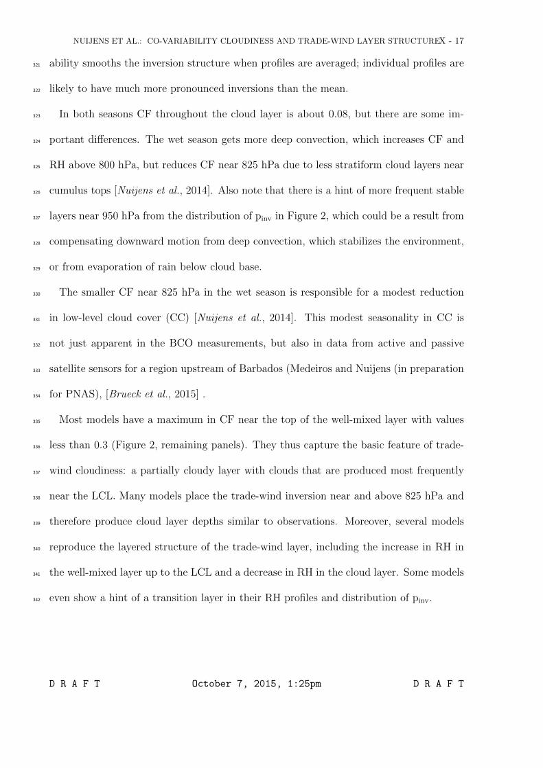
ability smooths the inversion structure when profiles are averaged; individual profiles are321
likely to have much more pronounced inversions than the mean.322
In both seasons CF throughout the cloud layer is about 0.08, but there are some im-323
portant differences. The wet season gets more deep convection, which increases CF and324
RH above 800 hPa, but reduces CF near 825 hPa due to less stratiform cloud layers near325
cumulus tops [Nuijens et al., 2014]. Also note that there is a hint of more frequent stable326
layers near 950 hPa from the distribution of pinv in Figure 2, which could be a result from327
compensating downward motion from deep convection, which stabilizes the environment,328
or from evaporation of rain below cloud base.329
The smaller CF near 825 hPa in the wet season is responsible for a modest reduction330
in low-level cloud cover (CC) [Nuijens et al., 2014]. This modest seasonality in CC is331
not just apparent in the BCO measurements, but also in data from active and passive332
satellite sensors for a region upstream of Barbados (Medeiros and Nuijens (in preparation333
for PNAS), [Brueck et al., 2015] .334
Most models have a maximum in CF near the top of the well-mixed layer with values335
less than 0.3 (Figure 2, remaining panels). They thus capture the basic feature of trade-336
wind cloudiness: a partially cloudy layer with clouds that are produced most frequently337
near the LCL. Many models place the trade-wind inversion near and above 825 hPa and338
therefore produce cloud layer depths similar to observations. Moreover, several models339
reproduce the layered structure of the trade-wind layer, including the increase in RH in340
the well-mixed layer up to the LCL and a decrease in RH in the cloud layer. Some models341
even show a hint of a transition layer in their RH profiles and distribution of pinv.342
D R A F T October 7, 2015, 1:25pm D R A F T

X - 18NUIJENS ET AL.: CO-VARIABILITY CLOUDINESS AND TRADE-WIND LAYER STRUCTURE
Many models are systematically too dry in the upper part of the cloud layer (850-825343
hPa), but most of them predict the warming and moistening towards the wet season.344
The associated changes in the CF profile at levels below 850 hPa are small, consistent345
with the observations. Models thus reproduce the robustness of the trade-wind layer.346
Nevertheless, no model stands out as performing particularly well at capturing the finer347
details, including the difference in LCL between the seasons, the invariance of CF near348
the LCL and most importantly, the decrease in CF near 825 hPa.349
These points will be discussed in more detail when we relate cloudiness to the structure350
of the trade-wind layer (section 4.2). First, we will take a closer look at how models vary351
the structure of cloud and humidity on shorter time scales.352
3.2. Short-term variability
How a model arrives at its mean CF profile can be very different from the observations.353
In the observations individual days experience clouds that are fairly evenly distributed354
over a layer from the LCL to the mean inversion height, whereas in the models the vertical355
distribution of clouds can differ substantially from one day to the next.356
The shape of the CF profile can be measured by a parameter γ = CFLCL / (CFLCL +357
CFALOFT), which represents how bottom-heavy (large γ) or top-heavy (small γ) the CF358
profile is (Brient et al., submitted to Climate Dynamics). Distributions of γ from daily359
CF profiles are shown in black in Figure 3 a (dry season) and d (wet season). Values for360
γ are always less than 0.6, which implies that CF is distributed across the cloud layer and361
tends to be emphasized near the top of the cloud layer especially in the dry season.362
Compared to observations, models differ greatly in their distributions of γ. Several363
models shift between very bottom-heavy (γ > 0.9) and top-heavy profiles (γ < 0.1). This364
D R A F T October 7, 2015, 1:25pm D R A F T

NUIJENS ET AL.: CO-VARIABILITY CLOUDINESS AND TRADE-WIND LAYER STRUCTUREX - 19
behaviour of γ is related to frequent occurrences of CFLCL = 0 or CFALOFT = 0 (square365
markers on the left outset of Figure 3b-c, e-f). However, in the observations there are366
very few days on which CF at either level is completely absent. This is even more true for367
CCLCL (in black solid lines) because it represents a cloud amount integrated over many368
observed heights within one model layer.369
In observations the total variance in CFALOFT is about twice that of CFLCL (see Table370
2, whose values were previously shown in Nuijens et al. [2015]). Hence, variability in371
cloudiness near the inversion is the dominant contributor to variability in low-level CC.372
In contrast, six out of nine models have in total more variance in CFLCL than in CFALOFT373
(Table 2), which is caused by their frequent dissipation of CF near the LCL.374
Periods with zero CFLCL can in some models last for days or weeks at a time [Nuijens375
et al., 2015], which suggests that the behaviour is not random. In the following sections,376
we analyze if such behaviour can be linked to the modeled trade-wind structure and377
large-scale flow.378
4. Patterns of co-variability of cloud and environment
The results presented in previous sections hint that patterns of co-variability between379
cloudiness and the environment are systematically different in the models compared to ob-380
servations. For CFLCL and CFALOFT respectively, section 4.1 and 4.2 reveal the anomalous381
profiles of RH, absolute humidity q, potential temperature θ, vertical velocity ω and the382
wind components u, v for months with large and small CF - in observations and models.383
The anomalies are taken with respect to a yearly running mean centered on each month.384
Furthermore, we perform regressions between CF and parameters that one may call385
large-scale predictors, which have been found important for explaining variations in cloudi-386
D R A F T October 7, 2015, 1:25pm D R A F T

X - 20NUIJENS ET AL.: CO-VARIABILITY CLOUDINESS AND TRADE-WIND LAYER STRUCTURE
ness in previous studies [Brueck et al., 2015]. These parameters include the RH averaged387
over the well-mixed layer (〈RH〉ML), the vertical difference in RH between 850 hPa and388
the LCL (∆CLRH = RH850-RHLCL) and the vertical difference in RH across the inversion389
layer (∆ILRH = RH700-RH850). Furthermore, the potential temperature lapse rate across390
the transition layer or mixed-layer top is considered, dθ/dzTL, which for the observations391
is derived between 1000 and 900 hPa and for the models between one model level above392
and below the LCL (which are not always separated by 100 hPa, hence we take the actual393
gradient here instead). The free tropospheric θ lapse rate is also considered, whereby ∆ILθ394
is determined between 750 and 600 hPa. Lastly, the vertical velocity at 825 hPa (ω825)395
and the near-surface wind speed UL0 are included.396
4.1. Cloudiness near the LCL
4.1.1. Observed versus modeled seasonal patterns397
In observations the differences in CF*LCL from one month to the next are generally398
modest, but there are a few notable differences. Months with larger CF*LCL (thick black399
lines, Figure 4) have a drier well-mixed layer, a relatively moist cumulus layer and a very400
dry and warm layer near and above the inversion between 825 hPa and 600 hPa compared401
to months with smaller CF*LCL (thin black lines). The dry and warm air between 825-402
600 hPa is likely associated with the intrusion of Saharan Dry Air layers, which occurs403
throughout late Spring and early summer [Carlson and Prospero, 1972].404
Relatively cold cloud layers over warm well-mixed layers destabilize the cloud layer to405
convection and triggers abundant cloudiness within the first 1.5 km above the LCL. The406
cloudiest months also have stronger winds, with a more pronounced northerly component,407
which is consistent with the air masses being relatively cold (in θ) and dry (in q). A408
D R A F T October 7, 2015, 1:25pm D R A F T

NUIJENS ET AL.: CO-VARIABILITY CLOUDINESS AND TRADE-WIND LAYER STRUCTUREX - 21
separation in the vertical wind component, ω, is only visible above 825 hPa, which suggests409
that months with large-scale subsidence generally have larger CF*LCL, but that ω is not410
a decisive factor.411
We have already seen that models tend to have more variance in CFLCL than is observed,412
with frequent occurrences of CFLCL = 0 (Table 2 and Figure 3c). Therefore it might not413
come as a surprise that models co-vary CFLCL with the environment in a number of414
ways. As the anomaly profiles for a subset of models illustrate, increases in humidity415
and temperature, winds and subsidence can either increase or decrease CFLCL (Figure 4).416
Some models are close to the observed behaviour (BCC, NCAR-C4), but have weaker and417
more southerly winds at times of large cloudiness instead. Other models show very little418
separation in profiles (MPIM-E62) or produce more CFLCL during months with mean419
rising motion (ω < 0) that have a moister and warmer trade-wind layer (ECMWF-LI,420
MOHC and NCAR-C5).421
In the following section we discuss the relationships of cloudiness with the environment422
in more detail by looking at daily and monthly time scales. To simplify the discussion we423
perform single and multi-variate regressions of cloudiness with the large-scale predictors424
defined above.425
426
4.1.2. Predictors of cloudiness427
To facilitate the comparison between models and observations, which differ in their428
magnitudes and in their variances of CF, a standardized regression is used whereby the429
regression coefficients are scaled by the ratio of the standard deviation of a parameter430
to the standard deviation of CF. Table 3 lists the parameter that explains most of the431
D R A F T October 7, 2015, 1:25pm D R A F T

X - 22NUIJENS ET AL.: CO-VARIABILITY CLOUDINESS AND TRADE-WIND LAYER STRUCTURE
variance, using a single regression for each parameter, as well as using a multi-variate432
regression, which basically removes the effect of covarying parameters that may strengthen433
or weaken individual relationships. The single regression coefficients are also plotted in434
Figure 5 for the different time scales. The regressions for different time scales are created435
by first removing the long-term mean before performing the regression. For instance,436
monthly means are subtracted from daily means and yearly means are subtracted from437
monthly means.438
The observed regressions for CF∗LCL turn out to be overall small and negligible for439
most parameters - including RH. Altogether the selected set of parameters explains 24%440
of the observed total variance on daily time scales and 56% of the observed total variance441
on monthly time scales. UL0 and dθ/dzTL are the parameters that best explain monthly442
variations in CF*LCL (30% each).443
All models run counter to the observations by producing excessive CFLCL when the well-444
mixed layer is relatively humid and topped by a more stable transition layer. 〈RH〉ML and445
dθ/dzTL explain at least half of the variance in monthly CFLCL (last column, Table 3).446
In addition, the models lack the observed relationships between CFLCL and UL0, or that447
relationship has the opposite sign.448
The time series in Figure 6 illustrate the relationship between CFLCL and RH in obser-449
vations (top two panels) and a few models for which the regression coefficients between450
CFLCL and 〈RH〉ML are larger than 0.7 at monthly time scales. The observations show that451
CCLCL has day-to-day variations, but stays close to 20% on longer time scales. Although452
co-variations between daily RHLCL and CFLCL can be observed, CFLCL does not exhibit453
the multi-day (i.e., synoptic) fluctuations that RH does. The models’ single-timestep be-454
D R A F T October 7, 2015, 1:25pm D R A F T

NUIJENS ET AL.: CO-VARIABILITY CLOUDINESS AND TRADE-WIND LAYER STRUCTUREX - 23
havior shows that their variances in CFLCL are much larger than observed, which in some455
models (e.g., MPIM-E62) are tightly linked to RH variations (cf. Figure 5).456
Behind the behavior we derive from the models appears to linger well-established re-457
lationships between low-level cloudiness, relative humidity, the stability of the lower at-458
mosphere and the large-scale vertical velocity, which in climatologies separate patterns of459
cloudiness along latitude and inspired cloud parameterizations decades ago. For example,460
many climate models use a diagnostic cloud scheme whereby CF is some function of the461
RH, assuming that condensation on sub-grid scales is related to a larger scale synoptic462
regime that makes an imprint on the mean relative humidity [Slingo, 1980; Sundqvist463
et al., 1989; Qu et al., 2014]. Larger cloud amounts, such as belonging to stratocumulus464
decks, have also been linked to regions with enhanced lower tropospheric stability [Klein465
and Hartmann, 1993]. Therefore, vertical temperature gradients, as well as vertical veloc-466
ity ω, have likely made their way into parameterizations of cloudiness. However, because467
these parameters do not reflect the dominant mechanisms that control CF on shorter time468
scales, they might lead to overly strong dependencies.469
In the following section we explain why relationships between CF∗LCL and the large-scale470
environment are small on short time scales in the observations. We hypothesize about the471
underlying processes that lead to the observed relationships with UL0 and dθ/dzTL and dis-472
cuss reasons for the somewhat counterintuitive result that 〈RH〉ML plays only a minor role.473
474
4.1.3. Constraints on cloudiness near the LCL in nature475
In the observations there is little evidence for strong controlling factors on CF∗LCL.476
One of the explanations for this is that CF∗LCL,when averaged over a day or longer has477
D R A F T October 7, 2015, 1:25pm D R A F T
X - 24NUIJENS ET AL.: CO-VARIABILITY CLOUDINESS AND TRADE-WIND LAYER STRUCTURE
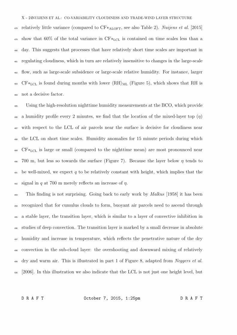
relatively little variance (compared to CF∗ALOFT, see also Table 2). Nuijens et al. [2015]478
show that 60% of the total variance in CF∗LCL is contained on time scales less than a479
day. This suggests that processes that have relatively short time scales are important in480
regulating cloudiness, which in turn are relatively insensitive to changes in the large-scale481
flow, such as large-scale subsidence or large-scale relative humidity. For instance, larger482
CF∗LCL is found during months with lower 〈RH〉ML (Figure 5), which shows that RH is483
not a decisive factor.484
Using the high-resolution nighttime humidity measurements at the BCO, which provide485
a humidity profile every 2 minutes, we find that the location of the mixed-layer top (η)486
with respect to the LCL of air parcels near the surface is decisive for cloudiness near487
the LCL on short time scales. Humidity anomalies for 15 minute periods during which488
CF∗LCL is large or small (compared to the nighttime mean) are most pronounced near489
700 m, but less so towards the surface (Figure 7). Because the layer below η tends to490
be well-mixed, we expect q to be relatively constant with height, which implies that the491
signal in q at 700 m merely reflects an increase of η.492
This finding is not surprising. Going back to early work by Malkus [1958] it has been493
recognized that for cumulus clouds to form, buoyant air parcels need to ascend through494
a stable layer, the transition layer, which is similar to a layer of convective inhibition in495
studies of deep convection. The transition layer is marked by a small decrease in absolute496
humidity and increase in temperature, which reflects the penetrative nature of the dry497
convection in the sub-cloud layer: the overshooting and downward mixing of relatively498
dry and warm air. This is illustrated in part 1 of Figure 8, adapted from Neggers et al.499
[2006]. In this illustration we also indicate that the LCL is not just one height level, but500
D R A F T October 7, 2015, 1:25pm D R A F T
NUIJENS ET AL.: CO-VARIABILITY CLOUDINESS AND TRADE-WIND LAYER STRUCTUREX - 25
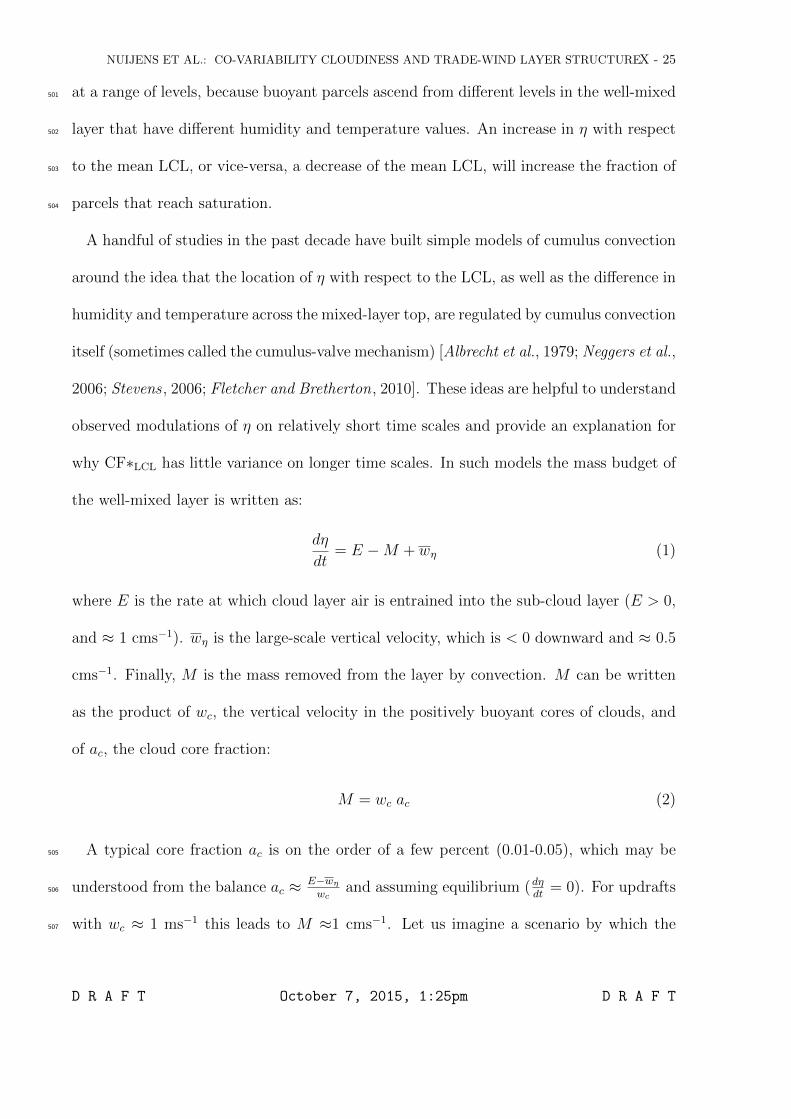
at a range of levels, because buoyant parcels ascend from different levels in the well-mixed501
layer that have different humidity and temperature values. An increase in η with respect502
to the mean LCL, or vice-versa, a decrease of the mean LCL, will increase the fraction of503
parcels that reach saturation.504
A handful of studies in the past decade have built simple models of cumulus convection
around the idea that the location of η with respect to the LCL, as well as the difference in
humidity and temperature across the mixed-layer top, are regulated by cumulus convection
itself (sometimes called the cumulus-valve mechanism) [Albrecht et al., 1979; Neggers et al.,
2006; Stevens , 2006; Fletcher and Bretherton, 2010]. These ideas are helpful to understand
observed modulations of η on relatively short time scales and provide an explanation for
why CF∗LCL has little variance on longer time scales. In such models the mass budget of
the well-mixed layer is written as:
dη
dt= E −M + wη (1)
where E is the rate at which cloud layer air is entrained into the sub-cloud layer (E > 0,
and ≈ 1 cms−1). wη is the large-scale vertical velocity, which is < 0 downward and ≈ 0.5
cms−1. Finally, M is the mass removed from the layer by convection. M can be written
as the product of wc, the vertical velocity in the positively buoyant cores of clouds, and
of ac, the cloud core fraction:
M = wc ac (2)
A typical core fraction ac is on the order of a few percent (0.01-0.05), which may be505
understood from the balance ac ≈ E−wηwc
and assuming equilibrium (dηdt
= 0). For updrafts506
with wc ≈ 1 ms−1 this leads to M ≈1 cms−1. Let us imagine a scenario by which the507
D R A F T October 7, 2015, 1:25pm D R A F T

X - 26NUIJENS ET AL.: CO-VARIABILITY CLOUDINESS AND TRADE-WIND LAYER STRUCTURE
well-mixed layer is perturbed and q increases by δq, which lowers the LCL and leads to508
a ten-fold increase in ac (#1 and 2, Figure 8). Following Equation 2, M consequently509
increases by an order of magnitude to 10 cms−1, which has the potential to lower η by a510
100 m in only 1000 s. The net effect is to lower η, bringing it closer to the mean LCL511
again, which constitutes the negative feedback. At the same time, the amount of dry air512
that is pushed down by convective downdrafts helps increase the stability by increasing513
∆TLq. Both processes lead to a reduction in the fraction of air parcels that saturate, which514
reduces M and brings the well-mixed layer to a new equilibrium state (# 3 in Figure 8).515
Note that a difference exists between the cloud core fraction ac and the actual CF. CF is516
determined by all cloudy air parcels, including those that are negatively buoyant, whereas517
ac only includes the fraction of positively buoyant parcels. LES indicates that values for518
CF are a factor 2 to 10 larger than ac [Siebesma et al., 2003; VanZanten et al., 2011]. What519
might control differences between the two warrants further investigation, but at first order520
we may assume that the two are proportional and postulate that because convection acts521
to keep η and the LCL close to one another [Albrecht et al., 1979], variations in CF∗LCL522
are also limited.523
Using this framework, it can be understood that the RH in the well-mixed layer can524
help regulate the LCL and thus CF∗LCL on shorter time scales. However, such local525
variations are poorly encapsulated in the RH averaged over a day or longer. Why we526
do not see a stronger relationship with RH on even shorter time scales (not shown) is527
somewhat surprising, and in contrast with studies that have successfully linked humidity528
and temperature variations to cloudiness, most notably the work by [Tompkins , 2002] on529
statistical (PDF) cloud schemes. The temporal resolution of the measurements may play530
D R A F T October 7, 2015, 1:25pm D R A F T

NUIJENS ET AL.: CO-VARIABILITY CLOUDINESS AND TRADE-WIND LAYER STRUCTUREX - 27
a role: although the updrafts and downdrafts are likely resolved, the larger humidity in531
the core of the updraft may not be. Furthermore, temperature fluctuations that matter532
to cloudiness on short time scales are not resolved.533
There appear to be mechanisms that may change CF∗LCL on monthly time scales:534
namely, dθ/dzTL has a negative relationship with CF∗LCL and UL0 has a positive relation-535
ship with CF∗LCL. These relationships may be understood from Equation 1 by noting that536
different equilibria (dηdt
= 0) are possible. Larger dθ/dzTL may correspond to a smaller en-537
trainment rate E and hence a smaller η, which would correspond to smaller ac. As for the538
wind speed, which has appeared as an important factor in numerous studies [Klein, 1997;539
Brueck et al., 2015], but generally receives less attention compared to thermodynamic540
arguments: an increase in UL0 linearly increases the surface buoyancy flux Fb,s. Energeti-541
cally, the effect of larger Fb,s is to increase the depth of the well-mixed layer η (through an542
increase in E): that deeper layer allows the vertical gradient of the buoyancy flux, which543
determines the local heating rate, to remain unchanged, in order to balance an unchanged544
radiative cooling rate [Nuijens and Stevens , 2012]. Thermodynamically, the effect of a545
larger wind speed is to lower the LCL. This is due to a decrease in the Bowen ratio and546
an increase in RH, due to a larger increase in the surface latent heat flux compared to547
the surface sensible flux, the latter being limited by the entrainment of relatively warm548
air [Albrecht et al., 1979; Betts and Ridgway , 1989]. The increase in η through energetic549
constraints and the decrease in LCL through thermodynamic constraints would increase550
cloudiness. Other possibilities through which stronger winds may impact cloudiness are551
when they are accompanied by increased convergence, either locally, or when the ITCZ is552
located at higher latitudes in boreal summer (assuming that winds vanish at the ITCZ).553
D R A F T October 7, 2015, 1:25pm D R A F T
X - 28NUIJENS ET AL.: CO-VARIABILITY CLOUDINESS AND TRADE-WIND LAYER STRUCTURE
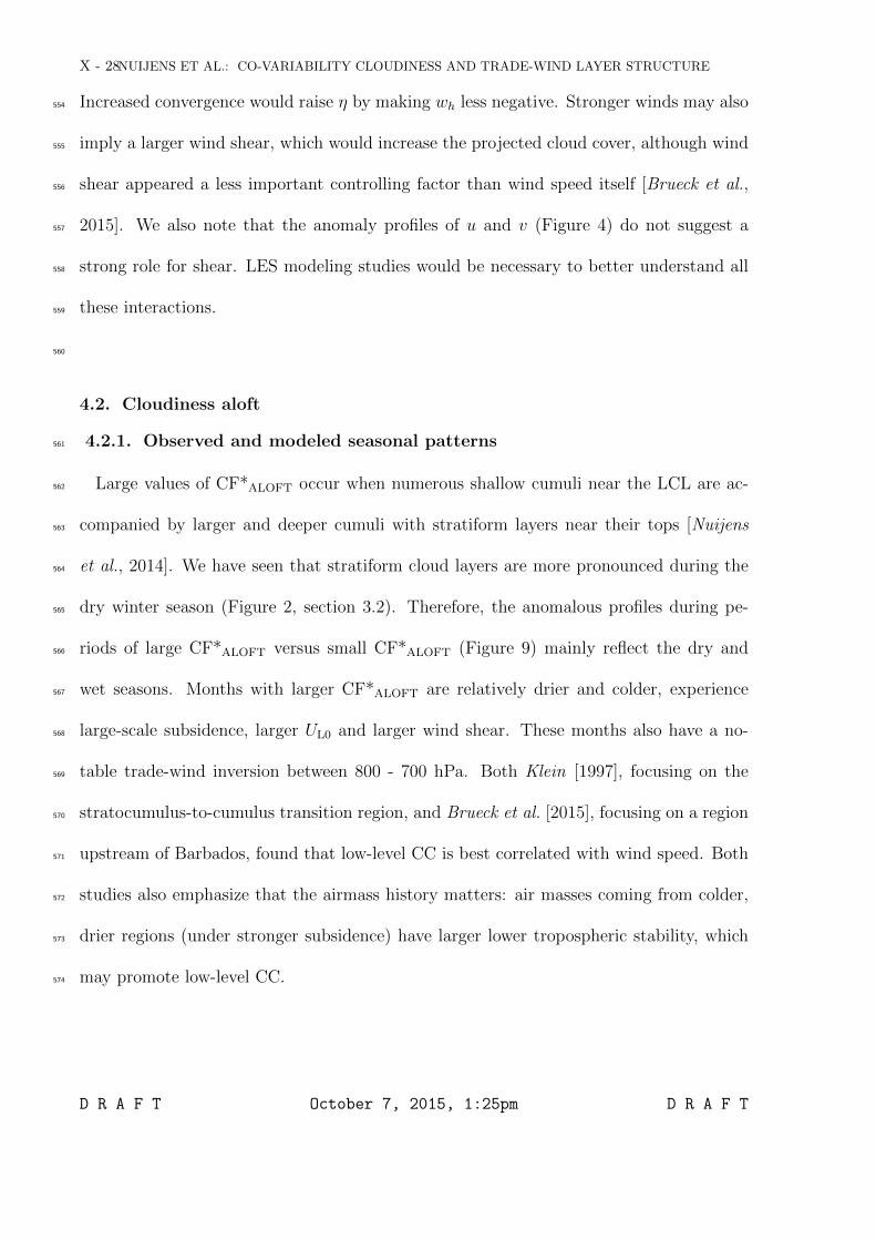
Increased convergence would raise η by making wh less negative. Stronger winds may also554
imply a larger wind shear, which would increase the projected cloud cover, although wind555
shear appeared a less important controlling factor than wind speed itself [Brueck et al.,556
2015]. We also note that the anomaly profiles of u and v (Figure 4) do not suggest a557
strong role for shear. LES modeling studies would be necessary to better understand all558
these interactions.559
560
4.2. Cloudiness aloft
4.2.1. Observed and modeled seasonal patterns561
Large values of CF*ALOFT occur when numerous shallow cumuli near the LCL are ac-562
companied by larger and deeper cumuli with stratiform layers near their tops [Nuijens563
et al., 2014]. We have seen that stratiform cloud layers are more pronounced during the564
dry winter season (Figure 2, section 3.2). Therefore, the anomalous profiles during pe-565
riods of large CF*ALOFT versus small CF*ALOFT (Figure 9) mainly reflect the dry and566
wet seasons. Months with larger CF*ALOFT are relatively drier and colder, experience567
large-scale subsidence, larger UL0 and larger wind shear. These months also have a no-568
table trade-wind inversion between 800 - 700 hPa. Both Klein [1997], focusing on the569
stratocumulus-to-cumulus transition region, and Brueck et al. [2015], focusing on a region570
upstream of Barbados, found that low-level CC is best correlated with wind speed. Both571
studies also emphasize that the airmass history matters: air masses coming from colder,572
drier regions (under stronger subsidence) have larger lower tropospheric stability, which573
may promote low-level CC.574
D R A F T October 7, 2015, 1:25pm D R A F T

NUIJENS ET AL.: CO-VARIABILITY CLOUDINESS AND TRADE-WIND LAYER STRUCTUREX - 29
That said, the deeper clouds may occur during disturbed periods much shorter than a575
month, which deviate from the mean conditions during the dry season, a point which we576
return to in the next section.577
The models in Figure 9 diverge in their patterns. Some models resemble the observa-578
tions and have larger CFALOFT in the dry season (IPSL and ECMWF-LI) when the free579
troposphere is dry and warm and mean subsidence prevails. Other models show the op-580
posite: larger CFALOFT is produced at times of mean ascent, when the inversion is weaker581
and the lower troposphere is more humid (MRI, CNRM, MOHC and NCAR-C5). During582
those months the boundary layer overall appears to be much deeper and moister than583
what is typical for the trades.584
Similar to what we did for CFLCL we next compare the regressions of CFALOFT with585
a set of predictors to discuss the most apparent relationships across time scales in the586
observations and the models.587
588
4.2.2. Predictors of cloudiness589
On a day-to-day basis CF*ALOFT varies more strongly with RH in the cloud layer (mea-590
sured by ∆CLRH, which scales mostly with RH825) and with ω825 than what we have591
seen for CF*LCL. The fraction of variance explained by the selected set of predictors is592
also larger (0.44, compared to 0.24 for CF*LCL, Table 4). The stronger covariance can593
be explained because the main source of RH in the cloud layer is convection itself, which594
transports moisture out of the mixed-layer into the free troposphere. This relationship is595
already present on time scales of minutes (Figure 7b) and explains why the daily regression596
coefficient between CF*ALOFT and ∆CLRH is relatively large at 0.5 (Figure 10).597
D R A F T October 7, 2015, 1:25pm D R A F T

X - 30NUIJENS ET AL.: CO-VARIABILITY CLOUDINESS AND TRADE-WIND LAYER STRUCTURE
Days with larger CF*ALOFT also correspond to weaker subsidence or larger mean ascent,598
so that the regression coefficient with ω825 is negative on daily time scales (Figure 10).599
This hints that synoptic disturbances, such as easterly waves, can promote CF*ALOFT600
even when on average that month experiences subsiding motion. Consistent with that re-601
lationship, the regression coefficient with ∆ILRH is positive on daily time scales, reflecting602
a deepening and moistening of the cloud layer.603
Also on monthly time scales the variance in CF*ALOFT is somewhat better explained by604
the selected set of predictors than the variance in CCLCL. However, the covariance with605
∆CLRH (RH825) is less pronounced, presumably because that covariance exists locally and606
is poorly encapsulated in longer averages. Parameters that do play an important role are607
∆ILθ and UL0. What may underlie these relationships is a greater potential for stratiform608
cloud layers to form under stronger inversions when surface evaporation is large [Nuijens609
and Stevens , 2012]. However, those conditions appear to be a prerequisite rather than610
a controlling factor, because neither covary strongly with CF*ALOFT on the shorter daily611
time scales.612
The results suggest that an important factor for increasing CF*ALOFT and CC is the613
potential for trade-wind cumuli to deepen, but nevertheless maintain a limited depth so614
that the trade-wind layer structure is preserved. If the trade-wind inversion becomes less615
defined because much deeper convection transports moisture all the way through the cloud616
and inversion layers into the free troposphere, such as during the wet season (Figure 2,617
light grey line), CFALOFT will decrease.618
All models agree with the observations that days with larger ∆CLRH and weaker sub-619
sidence correspond to larger CFALOFT (Figure 10). Yet whereas such parameters become620
D R A F T October 7, 2015, 1:25pm D R A F T

NUIJENS ET AL.: CO-VARIABILITY CLOUDINESS AND TRADE-WIND LAYER STRUCTUREX - 31
less important in the observations on monthly time scales or relationships between these621
parameters and CFALOFT change sign, the majority of models continue to show strong622
relationships with ∆CLRH and ω825. Models disagree on the sign of the relationship with623
ω825, which leads to opposing anomaly profiles (Figure 9). Some models produce the624
largest CFALOFT in the wet season with strongest mean ascent (MRI, CNRM), whereas625
others reproduce the observations by producing the largest CFALOFT in the dry season626
when strong inversions as well as stronger winds are present (ECMWF-LI, IPSL). Many627
models fail to reproduce the observed relationships with UL0 and ∆ILθ, although a few628
models capture at least the relationship with ∆ILθ (BCC, IPSL, NCAR-C4) or with UL0629
(ECMWF-LI).630
5. Discussion
We have identified some common biases of global (climate) models in how they vary631
trade-wind cloudiness with the environment. First, models have stronger than observed632
relationships between CFLCL and the RH in the well-mixed layer. We explained that in633
nature, variations in RH may regulate the LCL and thus be linked to cloud formation634
locally, but that these local signatures diminish over longer time scales. Furthermore,635
we explained how convection responds rapidly to perturbations in RH by ventilating the636
mixed-layer, which has a negative feedback on CFLCL (section 4.1.3). Apparently climate637
models do not represent such processes properly. Therefore, modeled CFLCL appears to638
be too sensitive to changes in RH.639
Second, models have stronger than observed relationships between CFLCL and the tem-640
perature stratification at the top of the well-mixed layer. Models produce larger CFLCL641
when the transition layer and lower cloud layer are more stratified, whereas in observations642
D R A F T October 7, 2015, 1:25pm D R A F T

X - 32NUIJENS ET AL.: CO-VARIABILITY CLOUDINESS AND TRADE-WIND LAYER STRUCTURE
larger cloudiness near the LCL is found when these layers are less stratified. Observations643
do show larger CFALOFT underneath a stronger trade-wind inversion further aloft, which644
many models do not reproduce.645
The models diverge in how they distribute CF and RH across the depth of the trade-646
wind layer. While some models reduce CFLCL as the RH in the cloud layer and CFALOFT647
increase, other models keep CFLCL unchanged or even increase it.648
We illustrate these different behaviours by means of Figures 11 and 12, which combine649
the behaviours of CFLCL and CFALOFT seen in Figure 5 and 10. The panels in Figure650
11 represent how parameters differ between days with a uniform distribution of moisture651
across the cloud layer and days with a less uniform distribution of moisture, whereby the652
latter is measured by ∆CLRH. These differences, δ’s, are derived as follows: we order all653
days by ∆CLRH, from high to low values, and select the upper and lower quartiles of days.654
Because ∆CLRH is generally negative, the upper quartile corresponds to small negative655
∆CLRH (well-mixed) and the lower quartile to large negative ∆CLRH (larger gradients656
in RH throughout the cloud layer). δ ≡ φupper − φlower corresponds to the difference657
in a parameter φ between those two quartiles, whereby φupper is the average φ over the658
upper quartile or days (and similar for the lower quartile). The grey shaded box indicates659
negative δ’s.660
The range of values for δ(∆CLRH) on the x-axis (20 - 70%) illustrates that models661
have a much larger variance in RH gradients in the cloud layer than the observations662
suggest. Nevertheless, both observations and models agree that days with largest ∆CLRH663
correspond to larger CFALOFT and that the actual change in CF, which is less than 0.2, is664
modest (Figure 11a). In observations those changes are accompanied by a small increase665
D R A F T October 7, 2015, 1:25pm D R A F T

NUIJENS ET AL.: CO-VARIABILITY CLOUDINESS AND TRADE-WIND LAYER STRUCTUREX - 33
in CFLCL (Figure11b). A number of models instead show a large decrease in CFLCL666
that falls into the grey shaded area. These models have the largest decreases in γ∗, which667
indicates that the models switch from bottom- to top-heavy profiles (δγ < 0, (Figure11c)),668
whereas in observations the CF profile becomes only slightly more top-heavy (remember669
also Figure 3). Because some of these models (MPIM-E62, CCCma) have large CFLCL670
to begin with, and little to no CFALOFT, these changes can be quite effective at reducing671
low-level CC overall. The same models also show that the RH in the mixed-layer decreases672
(δ〈RH〉ML < 0, Figure11d) when the distribution of RH in the cloud layer becomes more673
uniform.674
Brient et al. (submitted to Climate Dynamics) show that models that produce a bottom-675
heavy profile more effectively reduce cloudiness as climate warms and therefore have a high676
climate sensitivity. Our findings suggest that these models exhibit stronger relationships677
between CF and RH near the LCL than in observations. These models tend to shift678
cloud layers near the LCL to levels further aloft when moisture is mixed upward and the679
cumulus layer deepens, rather than sustaining cloudiness everywhere within the cumulus680
layer. The negative relationship between RH or CF near the inversion (850 hPa) and681
CF near the LCL is also apparent in a larger sample of CMIP models over all ocean682
regions that experience moderate subsidence or weak ascent (Medeiros and Nuijens, in683
preparation for PNAS).684
Sherwood et al. [2014] furthermore show that the simulated vertical moisture structure685
over tropical oceans in present-day climate separates high from low climate sensitivity686
models. They use ∆ILRH as a measure of lower tropospheric mixing and relate models687
with a small ∆ILRH to a high climate sensitivity. By diagnosing ∆ILRH only over the688
D R A F T October 7, 2015, 1:25pm D R A F T

X - 34NUIJENS ET AL.: CO-VARIABILITY CLOUDINESS AND TRADE-WIND LAYER STRUCTURE
western Pacific warm pool, where mean ascent dominates, they ensure that convection689
is indeed the lead effect on moisture at those levels, rather than variations in large-scale690
descent. They then argue that those models that sustain small ∆ILRH are apparently very691
effective at mixing moisture all the way from the well-mixed layer to the free troposphere692
(700 hPa). Presumably, as this mixing increases with global mean temperature CFLCL693
disappears.694
We find that models that are effective at mixing moisture by the definition of Sherwood695
et al. [2014] are indeed those that readily dissipate clouds near the LCL in the present-696
day climate. These are the models in Figure 11 that reduce temperature and moisture697
gradients throughout the lower troposphere as they reduce CFLCL. An illustration of698
this behaviour using the MPIM-E62 model as an example is shown in Figure 12b. The699
potential temperature difference across the inversion layer decreases (δ∆ILθ <0) and so700
does the temperature stratification across the transition layer (δ∆TLθ < 0). Furthermore,701
the RH difference across the inversion layer decreases (δ∆ILRH > 0, because ∆ILRH702
becomes less negative).703
This behavior contrasts with other models, which distribute RH and CF more uniformly704
across the cloud layer, so that as CFALOFT increases, CFLCL changes little or increases by705
a small amount (MOHC, NCAR-C5, ECMWF-LI). The MOHC model is used to illustrate706
this behaviour (Figure 12c). These models tend to maintain the structure of the trade-707
wind layer, in terms of layers separated by gradients. The associated larger temperature708
stratification in the transition layer in these models (δ dθ/dzTL > 0) may provide an709
additional mechanism through which moisture is capped within the well-mixed layer,710
which sustains cloud layers there. On the other hand, these models have a much stronger711
D R A F T October 7, 2015, 1:25pm D R A F T

NUIJENS ET AL.: CO-VARIABILITY CLOUDINESS AND TRADE-WIND LAYER STRUCTUREX - 35
than observed positive relationship between CFLCL and large-scale ascent (Figure 5). Of712
the models that we have analyzed here, the BCC, NCAR -C4 and MRI models have a713
low climate sensitivity in Sherwood et al. [2014]. In turn, high climate sensitivity models714
in Sherwood et al. [2014] include the MPIM-E62, IPSL, CCCma and CNRM models.715
In observations, neither a large decrease nor a large increase in CFLCL is evident when716
large-scale vertical motion or RH in the cloud layer changes. However, it would be easy to717
misjudge a model’s behavior as being more realistic, and therefore its climate sensitivity718
as more trustworthy, by means of a single process such as vertical moisture mixing. There719
is no model that stands out by reproducing observed relationships in all respects. The720
climate models that we have analysed here for instance lack either constraints on CFLCL721
due to convection, a sensitivity to wind speed and the strength of the trade-wind inversion,722
or an insensitivity to large-scale vertical velocity on longer time scales. Because changes723
in cloudiness will be a combined response to changes in a variety of factors (see also724
Bretherton et al. [2013]), many of which are connected through circulations and some of725
which are regulated by convection itself, a better understanding of the role of large-scale726
circulations versus the role of convection deserves more attention.727
6. Summary and conclusions
We evaluated global (climate) models for their ability to reproduce observed patterns of728
co-variability between the structure of the trade-wind layer, cloudiness and the thermo-729
dynamic and kinetic environment. A ground-based measurement site established on the730
Island of Barbados has provided the data required to study such variability in detail. We731
used these measurements for a period of up to four years and compared them to multi-year732
single-timestep output from models at a single site near or upstream of Barbados. The733
D R A F T October 7, 2015, 1:25pm D R A F T
X - 36NUIJENS ET AL.: CO-VARIABILITY CLOUDINESS AND TRADE-WIND LAYER STRUCTURE
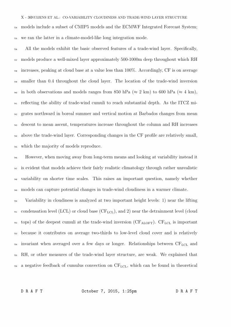
models include a subset of CMIP5 models and the ECMWF Integrated Forecast System;734
we ran the latter in a climate-model-like long integration mode.735
All the models exhibit the basic observed features of a trade-wind layer. Specifically,736
models produce a well-mixed layer approximately 500-1000m deep throughout which RH737
increases, peaking at cloud base at a value less than 100%. Accordingly, CF is on average738
smaller than 0.4 throughout the cloud layer. The location of the trade-wind inversion739
in both observations and models ranges from 850 hPa (≈ 2 km) to 600 hPa (≈ 4 km),740
reflecting the ability of trade-wind cumuli to reach substantial depth. As the ITCZ mi-741
grates northward in boreal summer and vertical motion at Barbados changes from mean742
descent to mean ascent, temperatures increase throughout the column and RH increases743
above the trade-wind layer. Corresponding changes in the CF profile are relatively small,744
which the majority of models reproduce.745
However, when moving away from long-term means and looking at variability instead it746
is evident that models achieve their fairly realistic climatology through rather unrealistic747
variability on shorter time scales. This raises an important question, namely whether748
models can capture potential changes in trade-wind cloudiness in a warmer climate.749
Variability in cloudiness is analyzed at two important height levels: 1) near the lifting750
condensation level (LCL) or cloud base (CFLCL), and 2) near the detrainment level (cloud751
tops) of the deepest cumuli at the trade-wind inversion (CFALOFT). CFLCL is important752
because it contributes on average two-thirds to low-level cloud cover and is relatively753
invariant when averaged over a few days or longer. Relationships between CFLCL and754
RH, or other measures of the trade-wind layer structure, are weak. We explained that755
a negative feedback of cumulus convection on CFLCL, which can be found in theoretical756
D R A F T October 7, 2015, 1:25pm D R A F T

NUIJENS ET AL.: CO-VARIABILITY CLOUDINESS AND TRADE-WIND LAYER STRUCTUREX - 37
models of convection, appears present in the observations. In this negative feedback,757
cumulus convection acts like a valve on top of the well-mixed layer that removes mass758
as soon as cloud formation is abundant. This mechanisms maintains the height of the759
mixed-layer top in the vicinity of the LCL, which in turn constraints CF.760
CFALOFT on the other hand is important because it contributes most to the variance761
in low-level cloud cover. CF at this level covaries with the strength of the trade-wind762
inversion and with surface wind speed on monthly time scales, leading to larger CFALOFT763
in boreal winter, when the trade-winds are stronger and lower tropospheric stability is764
larger. However, variance in CFALOFT on shorter daily time scales is unexplained by these765
factors.766
None of the models that we analyzed stands out by reproducing the observations better767
in all respects. Almost all models overestimate the variance in CFLCL compared to the768
variance in CFALOFT on shorter (daily) timescales. The large variance in modeled CFLCL769
lies in stronger than observed relationships between CFLCL and RH in the well-mixed770
layer. Furthermore, whereas in nature modest decreases in CFLCL are observed when the771
temperature stratification in the transition layer is larger (and convection is limited), the772
models show larger CFLCL under such conditions instead.773
Most models do not indicate that the strength of the inversion and the surface wind774
speed can promote CFALOFT in boreal winter. Models diverge in how they distribute CF775
and RH vertically across the trade-wind layer and in particular in response to changes776
in large-scale vertical motion. One group of models places most cloud layers near the777
LCL in a shallow layer with large CF. Cloud layers aloft are produced when moisture is778
transported away from the surface to levels near and above the inversion. This dries the779
D R A F T October 7, 2015, 1:25pm D R A F T

X - 38NUIJENS ET AL.: CO-VARIABILITY CLOUDINESS AND TRADE-WIND LAYER STRUCTURE
mixed-layer and lower part of the cloud layer at the expense of CFLCL. A very bottom-780
heavy profile (no CFALOFT) is then exchanged for a very top-heavy profile (no CFLCL).781
These models behave like the ones that Sherwood et al. [2014] refers to as models with782
a large vertical mixing potential, which effectively dry the mixed layer and cloud layer783
when climate warms. These models appear to reduce cloudiness, especially near the LCL,784
too eagerly when vertical mixing increases. Another group of models distributes RH and785
CF more uniformly across the cloud layer, so that CF near the LCL is maintained when786
moisture is mixed upwards and CF aloft increases. However, this increase is strongly787
linked to periods of mean ascent, which is unsupported by the observations.788
Modeled cloud changes in present-day climate thus appear to have a larger susceptibility789
to changes in their environment than the observations. This highlights that cloudiness in790
models is not entirely regulated by the processes that underlie variations in cloudiness in791
nature, which decreases our confidence that climate models can realistically predict the792
response of trade-wind clouds to increasing global temperatures.793
Acknowledgments. The BCO infrastructure is maintained by Ilya Serikov, Lutz794
Hirsch, Friedhelm Jansen, Bjoern Bruegmann, Monika Pfeiffer and Holger Linne, and795
without them this work would not have been possible. Many thanks go to Bjorn Stevens796
and Robert Pincus for helpful discussions on earlier versions of the manuscript. We also797
thank Rodrigo Colpo for his work on the CMIP5 output, Sebastian Massart for his help798
with retrieving IFS data, Andrew Gettelman for retrieving the BOMEX cfSites output799
for CAM4 and CAM5 and Jobst Musse for compiling the CALIOP data in Figure 1. Two800
reviewers greatly helped to improve the readability of the manuscript. LN appreciates801
the hospitality of NCAR and ECMWF during part of this work. BM acknowledges sup-802
D R A F T October 7, 2015, 1:25pm D R A F T

NUIJENS ET AL.: CO-VARIABILITY CLOUDINESS AND TRADE-WIND LAYER STRUCTUREX - 39
port by the Regional and Global Climate Modeling Program of the U.S. Department of803
Energy’s Office of Science, Cooperative Agreement DE-FC02-97ER62402. NCAR is spon-804
sored by the National Science Foundation. The BCO data, the ECMWF long integra-805
tions and the cfSites output for MPIM-E62, CAM4, CAM5 are available upon contacting806
the first author. The cfSites output for the remaining models can be downloaded from:807
http://cmip-pcmdi.llnl.gov/cmip5/data portal.html.808
References
Albrecht, B., A. Betts, W. Schubert, and S. Cox (1979), A model of the thermodynamic809
structure of the trade-wind boundary layer. part i: Theoretical formulation and sensi-810
tivity tests, J. Atmos. Sci., 36, 73–89.811
Betts, A., and W. Ridgway (1989), Climatic equilibrium of the atmospheric convective812
boundary layer over a tropical ocean, J. Atmos. Sci., 46, 2621–2641.813
Bony, S., and J.-L. Dufresne (2005), Marine boundary layer clouds at the heart of tropical814
cloud feedback uncertainties in climate models, Geophysical Research Letters, 32 (20),815
L20,806, doi:10.1029/2005GL023851.816
Bony, S., and K. A. Emanuel (2001), A Parameterization of the Cloudiness Associated817
with Cumulus Convection ; Evaluation Using TOGA COARE Data, J. Atmos. Sci, 58,818
3158–3183.819
Bretherton, C. S., P. N. Blossey, and C. R. Jones (2013), Mechanisms of marine low cloud820
sensitivity to idealized climate perturbations: A single-LES exploration extending the821
CGILS cases, Journal of Advances in Modeling Earth Systems, 5 (2), 316–337, doi:822
10.1002/jame.20019.823
D R A F T October 7, 2015, 1:25pm D R A F T

X - 40NUIJENS ET AL.: CO-VARIABILITY CLOUDINESS AND TRADE-WIND LAYER STRUCTURE
Brueck, H. M., L. Nuijens, and B. Stevens (2015), On the seasonal and synoptic timescale824
variability in low level cloudiness in the North Atlantic trades, J. Atmos. Sci., 72, 1428825
– 1446.826
Carlson, T. N., and J. M. Prospero (1972), The Large-Scale Movement of Saharan Air Out-827
breaks over the Northern Equatorial Atlantic, Journal of Applied Meteorology, 11 (2),828
283–297, doi:10.1175/1520-0450(1972)011¡0283:TLSMOS¿2.0.CO;2.829
Emanuel, K. (1993), A cumulus representation based on the episodic mixing model: the830
importance of mixing and microphysics in predicting humidity, in The representation of831
Cumulus Convection in Numerical Models. Meteorological Monographs, vol. 24, edited832
by K. Emanuel and D. J. Raymond, chap. 19, pp. 185–194, American Meteorological833
Society, Boston.834
Fletcher, J. K., and C. S. Bretherton (2010), Evaluating Boundary LayerBased Mass Flux835
Closures Using Cloud-Resolving Model Simulations of Deep Convection, J. Atmos. Sci.,836
67 (7), 2212–2225, doi:10.1175/2010JAS3328.1.837
Gettelman, A., M. I. Hegglin, S.-W. Son, J. Kim, M. Fujiwara, T. Birner, S. Kremser,838
M. Rex, J. A. Ael, H. Akiyoshi, J. Austin, S. Bekki, P. Braesike, C. Brhl, N. Butchart,839
M. Chipperfield, M. Dameris, S. Dhomse, H. Garny, S. C. Hardiman, P. Jckel, D. E.840
Kinnison, J. F. Lamarque, E. Mancini, M. Marchand, M. Michou, O. Morgenstern,841
S. Pawson, G. Pitari, D. Plummer, J. A. Pyle, E. Rozanov, J. Scinocca, T. G. Shepherd,842
K. Shibata, D. Smale, H. Teyssdre, and W. Tian (2010), Multi-model assessment of843
the upper troposphere and lower stratosphere: Tropics and global trends, Journal of844
Geophysical Research: Atmospheres, 115 (D3), n/a–n/a, doi:10.1029/2009JD013638.845
D R A F T October 7, 2015, 1:25pm D R A F T

NUIJENS ET AL.: CO-VARIABILITY CLOUDINESS AND TRADE-WIND LAYER STRUCTUREX - 41
Gregory, D., and P. R. Rowntree (1990), A Mass Flux Convection Scheme846
with Representation of Cloud Ensemble Characteristics and Stability-847
Dependent Closure, Mon. Weather Rev., 118 (7), 1483–1506, doi:10.1175/1520-848
0493(1990)118¡1483:AMFCSW¿2.0.CO;2.849
Klein, S. A. (1997), Synoptic Variability of Low-Cloud Properties and Meteorological850
Parameters in the Subtropical Trade Wind Boundary Layer, J. Climate, 10, 2018–2039.851
Klein, S. A., and D. L. Hartmann (1993), The seasonal cycle of low stratiform clouds, J.852
Climate, 6, 1587–1606.853
Lock, A. P. (2009), Factors influencing cloud area at the capping inversion for shallow854
cumulus clouds, Q. J. R. Meteor. Soc., 952 (April), 941–952, doi:10.1002/qj.855
Malkus, J. S. (1958), On the structure of the trade wind moist layer, Papers in physical856
oceanography and meteorology, 13 (2), 1–47.857
McFarlane, N., J. F. Scinocca, M. Lazare, R. Harvey, D. Verseghy, and J. Li (2005), The858
CCCma third generation atmospheric general circulation model (AGCM3), Canadian859
Centre for Climate Modelling and Analysis, Internal Report, 25pp.860
Medeiros, B., and B. Stevens (2011), Revealing differences in GCM representations of low861
clouds, Clim. Dyn., 36, 385–399.862
Medeiros, B., C. Antoniazzi, L. Nuijens, and B. Stevens (2010), Low-latitude bound-863
ary layer clouds as seen by CALIPSO, Journal of Geophysical Research, 115, doi:864
10.1029/2010JD014437.865
Neggers, R., B. Stevens, and J. D. Neelin (2006), A simple equilibrium model for shallow-866
cumulus-topped mixed layers, Theoretical and Computational Fluid Dynamics, 20 (5-6),867
305–322, doi:10.1007/s00162-006-0030-1.868
D R A F T October 7, 2015, 1:25pm D R A F T

X - 42NUIJENS ET AL.: CO-VARIABILITY CLOUDINESS AND TRADE-WIND LAYER STRUCTURE
Neggers, R. A. J., and A. P. Siebesma (2013), Constraining a System of Interacting869
Parameterizations through Multiple-Parameter Evaluation: Tracing a Compensating870
Error between Cloud Vertical Structure and Cloud Overlap, Journal of Climate, 26 (17),871
6698–6715, doi:10.1175/JCLI-D-12-00779.1.872
Neggers, R. a. J., a. P. Siebesma, and T. Heus (2012), Continuous Single-Column Model873
Evaluation at a Permanent Meteorological Supersite, Bulletin of the American Meteo-874
rological Society, 93 (9), 1389–1400, doi:10.1175/BAMS-D-11-00162.1.875
Nuijens, L., and B. Stevens (2012), The Influence of Wind Speed on Shallow Marine876
Cumulus Convection, J. Atmos. Sci., 69 (1), 168–184, doi:10.1175/JAS-D-11-02.1.877
Nuijens, L., I. Serikov, L. Hirsch, K. Lonitz, and B. Stevens (2014), The distribution and878
variability of low-level cloud in the North Atlantic trades, Q. J. R. Meteor. Soc., pp.879
n/a—-n/a, doi:10.1002/qj.2307.880
Nuijens, L., B. Medeiros, I. Sandu, and M. Ahlgrimm (2015), The behavior of trade-881
wind cloudiness in models and observations: The major cloud components and their882
variability, J. Adv. Model. Earth Syst., 07, doi:doi:10.1002/2014MS000390.883
Phillips, T. J., G. L. Potter, D. L. Williamson, R. T. Cederwall, J. S. Boyle, M. Fiorino,884
J. J. Hnilo, J. G. Olson, S. Xie, and J. J. Yio (2004), Evaluating Parameterizations in885
General Circulation Models: Climate Simulation Meets Weather Prediction, Bulletin886
of the American Meteorological Society, 85 (12), 1903–1915, doi:10.1175/BAMS-85-12-887
1903.888
Qu, X., A. Hall, S. Klein, and P. Caldwell (2014), On the spread of changes in marine889
low cloud cover in climate model simulations of the 21st century, Climate Dynamics,890
42 (9-10), 2603–2626, doi:10.1007/s00382-013-1945-z.891
D R A F T October 7, 2015, 1:25pm D R A F T

NUIJENS ET AL.: CO-VARIABILITY CLOUDINESS AND TRADE-WIND LAYER STRUCTUREX - 43
Rasch, P. J., and J. E. Kristjansson (1998), A comparison of the CCM3 model climate892
using diagnosed and predicted condensate parameterizations, J. Climate, 11, 1587–1614.893
Ricard, J. L., and J. F. Royer (1993), A statistical cloud scheme for use in an AGCM,894
Annales Geophysicae, 11, 1095–1115.895
Serikov, I., and S. Bobrovnikov (2010), Atmospheric temperature profiling with pure rota-896
tional raman lidars, in Recent Advances in Atmospheric Lidars, Optoelectronic materials897
and devices, vol. 7, edited by L. Fiorani and V. Mitev, pp. 149–216, INOE.898
Sherwood, S. C., S. Bony, and J.-L. Dufresne (2014), Spread in model climate sen-899
sitivity traced to atmospheric convective mixing, Nature, 505 (7481), 37–42, doi:900
10.1038/nature12829.901
Siebesma, A. P., C. S. Bretherton, A. Brown, A. Chlond, J. Cuxart, P. G. Duynkerke,902
H. Jiang, M. Khairoutdinov, D. Lewellen, C.-H. Moeng, E. Sanchez, B. Stevens,903
and D. E. Stevens (2003), A Large Eddy Simulation Intercomparison Study of904
Shallow Cumulus Convection, J. Atmos. Sci., 60 (10), 1201–1219, doi:10.1175/1520-905
0469(2003)60¡1201:ALESIS¿2.0.CO;2.906
Simmons, A., S. Uppala, D. Dee, and S. Kobayashi (2007), Era-interim: New ecmwf907
reanalysis products from 1989 onwards, ECMWF Newsletter, 110, 25–35.908
Slingo, J. M. (1980), A cloud parametrization scheme derived from GATE data for use909
with a numerical model, Q. J. R. Meteor. Soc., 106, 747–770.910
Slingo, J. M. (1987), The development and verification of a cloud prediction scheme for911
the ECMWF model, Q. J. R. Meteor. Soc., 113, 899–927.912
Stevens, B. (2006), Bulk boundary-layer concepts for simplified models of tropical913
dynamics, Theoretical and Computational Fluid Dynamics, 20 (5-6), 279–304, doi:914
D R A F T October 7, 2015, 1:25pm D R A F T

X - 44NUIJENS ET AL.: CO-VARIABILITY CLOUDINESS AND TRADE-WIND LAYER STRUCTURE
10.1007/s00162-006-0032-z.915
Stevens, B., A. S. Ackerman, B. A. Albrecht, A. R. Brown, A. Chlond, J. Cuxart, P. G.916
Duynkerke, D. C. Lewellen, M. K. Macvean, R. A. J. Neggers, E. Sanchez, A. P.917
Siebesma, and D. E. Stevens (2001), Simulations of Trade Wind Cumuli under a Strong918
Inversion, J. Atmos. Sci., 58 (14), 1870–1891.919
Sundqvist, H., E. Berge, and J. E. Kristjansson (1989), Condensation and cloud920
parameterization studies with a mesoscale numerical weather prediction model,921
Mon. Weather Rev., 117, 1641–1657.922
Tiedtke, M. (1989), A comprehensive mass flux scheme for cumulus parameterization in923
large-scale models, Mon. Weather Rev., 117, 1779–1800.924
Tiedtke, M. (1993), Representation of clouds in large-scale models, Mon. Weather Rev.,925
121, 3040–3061.926
Tompkins, A. M. (2002), A Prognostic Parameterization for the Subgrid-Scale Variability927
of Water Vapor and Clouds in Large-Scale Models and Its Use to Diagnose Cloud Cover,928
J. Atmos. Sci, 59 (12), 1917–1942.929
VanZanten, M. C., B. Stevens, L. Nuijens, A. P. Siebesma, A. S. Ackerman, F. Bur-930
net, A. Cheng, F. Couvreux, H. Jiang, M. Khairoutdinov, Y. Kogan, D. C. Lewellen,931
D. Mechem, K. Nakamura, A. Noda, B. J. Shipway, J. Slawinska, S. Wang, and A. Wys-932
zogrodzki (2011), Controls on precipitation and cloudiness in simulations of trade-wind933
cumulus as observed during RICO, Journal of Advances in Modeling Earth Systems,934
3 (2), M06,001, doi:10.1029/2011MS000056.935
Vial, J., J. L. Dufresne, and S. Bony (2013), On the interpretation of inter-model936
spread in CMIP5 climate sensitivity estimates, Clim. Dyn., 41, 3339–3362, doi:937
D R A F T October 7, 2015, 1:25pm D R A F T

NUIJENS ET AL.: CO-VARIABILITY CLOUDINESS AND TRADE-WIND LAYER STRUCTURE X - 45
DOI:10.1007/s00382-013-1725-9.938
von Salzen, K., N. McFarlane, and M. Lazare (2005), The role of shallow convection in939
the water and energy cycles of the atmosphere, Climate Dynamics, 25 (7-8), 671–688,940
doi:10.1007/s00382-005-0051-2.941
Webb, M., A. Lock, A. Bodas-Salcedo, S. Bony, J. Cole, T. Koshiro, H. Kawai, C. Lacagn-942
ina, F. Selten, R. Roehrig, and B. Stevens (2015), The diurnal cycle of marine cloud feed-943
back in climate models, Climate Dynamics, 44 (5-6), 1419–1436, doi:10.1007/s00382-944
014-2234-1.945
Wu, T., R. Yu, F. Zhang, Z. Wang, M. Dong, L. Wang, X. Jin, D. Chen, and L. Li946
(2010), The Beijing Climate Center atmospheric general circulation model: description947
and its performance for the present-day climate, Climate Dynamics, 34 (1), 123–147,948
doi:10.1007/s00382-008-0487-2.949
Yukimoto, S., Y. Adachi, M. Hosaka, T. Sakami, H. Yoshimura, M. Hirabara, T. Y.950
Tanaka, E. Shindo, H. Ysujino, M. Deushi, R. Mizuta, S. Yabu, A. Obata, H. Nakano,951
T. Koshiro, T. Ose, and A. Kitoh (2012), A new global climate model of the meteoro-952
logical research institute: Mri-cgcm3 model description and basic performance, Journal953
of the Meteorological Society of Japan. Ser. II, 90A, 23–64, doi:10.2151/jmsj.2012-A02.954
Zhang, G. J., and N. A. McFarlane (1995), Sensitivity of climate simulations to the pa-955
rameterization of cumulus convection in the canadian climate centre general circulation956
model, Atmosphere-Ocean, 33 (3), 407–446, doi:10.1080/07055900.1995.9649539, n/a.957
D R A F T October 7, 2015, 1:25pm D R A F T

X - 46 NUIJENS ET AL.: CO-VARIABILITY CLOUDINESS AND TRADE-WIND LAYER STRUCTURE
ground-based at BCOspace-borne near BCO
15 - 30 NH15 - 30 SH
inve
rsio
nLC
L
Figure 1. Lidar observations of the vertical distribution of cloud layer bases in the trades as
viewed from ground (in black) respectively from space (in blue). The distribution is made using
250 m bins and normalized by the total number of lidar profiles. It represents the frequency
(fraction) of finding a cloud layer base at a given height. The distribution in black is derived
from a laser ceilometer deployed at the BCO whose resolution corresponds to about 500 m. The
distribution from the CALIOP lidar in blue is determined over a 5x10◦ area just upstream of
Barbados at a 333 m footprint. We also show CALIOP distributions for the broader subtropics,
including all ocean between 15 and 30◦ in the Northern and Southern Hemisphere. These dis-
tributions illustrate that the cloud profile below 5 km is marked by two important height levels
where cloud layers tend to occur: near 700 m where cumuli have their base and near 1.5 - 2.5
km, where the inversion limits cumulus tops and stratiform layers can be found.
D R A F T October 7, 2015, 1:25pm D R A F T

NUIJENS ET AL.: CO-VARIABILITY CLOUDINESS AND TRADE-WIND LAYER STRUCTURE X - 47
No.
Abbrev
iationM
odel
Modelin
gC
enter
L600hPa/900hPa
cloud
/con
vectionsch
eme
1E
CW
MF
-LI
IFS
Lon
gin
tegrationE
urop
eanC
entre
forM
ediu
m-
24/
3Tiedtke
[1993]/
Ran
geW
eather
Forecasts
Tiedtke
[1989]2
MP
IM-E
63M
PI-E
SM
-LR
Max
-Plan
ckIn
stitute
for11
/2
Tiedtke
[1989]/
EC
HA
M6.3
Meteorology
Sundqvist
etal.
[1989]3
MP
IM-E
62M
PI-E
SM
-LR
Max
-Plan
ckIn
stitute
for11
/2
Tiedtke
[1989]/
EC
HA
M6.2
Meteorology
Sundqvist
etal.
[1989]4
BC
CB
CC
-CSM
1.1B
eijing
Clim
ateC
enter
7/
1Wuet
al.[2010]
/Slin
go[1987]
5C
CC
ma
Can
ESM
2C
anad
ianC
entre
forC
limate
14/
2von
Salzen
etal.
[2005]/
Modellin
gan
dA
naly
sis/M
cFarlan
eet
al.[2005]
6IP
SL
IPSL
-CM
5A-L
RIn
stitut
Pierre-S
imon
Lap
lace11
/1
Bon
yan
dEman
uel
[2001]/
Eman
uel
[1993]7
CN
RM
CN
RM
-CM
5C
entre
Nation
alde
Rech
erches
11/
2Gregory
andRow
ntree
[1990]/
Meteorologiq
ues
Ricard
andRoyer
[1993]8
MO
HC
Had
GE
M2-A
Met
Offi
ceH
adley
Cen
tre14
/2
Gregory
andRow
ntree
[1990]/
Lock
[2009]9
MR
IM
RI-C
GSM
3M
eteorologicalR
esearchIn
stitute
12/
1Yukim
otoet
al.[2012]
/Tiedtke
[1993]10
NC
AR
-C4
CA
M4
Nation
alC
enter
ofA
tmosp
heric
7/
1Rasch
andKristjan
sson[1998]
/R
esearchZhan
gan
dMcF
arlane
[1995]11
NC
AR
-C5
CA
M5
Nation
alC
enter
ofA
tmosp
heric
11/
2Gettelm
anet
al.[2010]
/R
esearchZhan
gan
dMcF
arlane
[1995]
Table
1.
List
ofm
odels
used
inth
ean
alysis,
inclu
din
gth
enum
ber
ofm
odel
levelsup
to600
hP
a(L
600hPa ),
and
betw
een
950-900hP
a(L
900hPa ),
and
references
toth
eirclou
dan
dcon
vectionsch
emes.
All
models
use
the
BO
ME
Xlo
cation,
excep
tth
e
EC
MW
F-L
I,M
PIM
-E63
and
MP
IM-E
62,w
hich
use
agrid
poin
tju
stupstream
ofB
arbad
os.A
llm
odels
have
outp
ut
every30
min
utes.
For
the
BC
Can
dN
CA
R-C
4m
odel
only
everysecon
dou
tput
stepis
used
inth
ean
alysis,
seesection
2.4.
D R A F T October 7, 2015, 1:25pm D R A F T

X - 48 NUIJENS ET AL.: CO-VARIABILITY CLOUDINESS AND TRADE-WIND LAYER STRUCTURE
Jan - Feb - MarSep - Oct - Nov
ILCLTLML
FT
Figure 2. Mean cloud and thermodynamic profiles are plotted, representative for the period
Jan - Mar (dry season) and Sep - Nov (wet season), from Barbados Cloud Observatory (BCO)
data and from model output for a location nearby Barbados (EMCWF-LI, MPIM-E63, MPIM-
E62) or the BOMEX location (all other models). Jan - Mar is depicted by solid lines, whereas
Sep - Nov is depicted by lighter-toned transparent lines. Variables shown from left to right:
cloud fraction (CF), the relative humidity (RH), the virtual potential temperature θv and the
frequency (fraction) of finding inversion layers at a given pressure level: pinv. Abbreviations for
the five layers that are identified in the BCO profiles refer to: ML = well-mixed layer, TL =
transition layer, CL = cloud (cumulus) layer, IL = inversion layer, FT = free troposphere.
D R A F T October 7, 2015, 1:25pm D R A F T

NUIJENS ET AL.: CO-VARIABILITY CLOUDINESS AND TRADE-WIND LAYER STRUCTURE X - 49
Jan - Feb - Mar
Sep - Oct - Nov
a b c
d e f
Figure 3. A parameter that measures the shape of the profile of CF and CF at selected levels
are shown for the period Jan - Mar (top row) and Sep - Nov (bottom row). The three panels are
frequency distributions of: a,d) γ∗, which represents how bottom-heavy (large γ) or top-heavy
(small γ) the CF profile is, modified after Brient et al. (submitted to Climate Dynamics); b,e)
CFLCL(Table 2); and c,f) CFALOFT. For definitions see section 2.5 and 3.2. The observed CFLCL
and CFALOFT are shown in dashed black lines and the observed CCLCL and CCALOFT are shown
separately in solid black lines. All parameters are derived from daily mean profiles. The minor
tick marks indicate the binning that is used. In c-d and f-g the bin 0 - 0.1 excludes the frequency
of finding CF = 0, these are shown separately by the square markers at the left outset of each
panel.
D R A F T October 7, 2015, 1:25pm D R A F T

X - 50 NUIJENS ET AL.: CO-VARIABILITY CLOUDINESS AND TRADE-WIND LAYER STRUCTURE
Figure 4. The anomalies in thermodynamic and kinetic profiles for months with large values of
CFLCL (thick lines) and small values of CFLCL (thin lines). The anomalies are taken with respect
to a yearly running mean centered on each month. In the top row, the BCO data are shown,
whereby the lines correspond to the lower and upper quartile of ordered anomalies in CCLCL
instead of CFLCL. The following rows show the same, but for the models using CFLCL. We show
only those models in which the variance in monthly CFLCL is better explained by parameters
that represent the large-scale state than in observations (Table 3).
D R A F T October 7, 2015, 1:25pm D R A F T

NUIJENS ET AL.: CO-VARIABILITY CLOUDINESS AND TRADE-WIND LAYER STRUCTURE X - 51
linea
r reg
ress
ion
coef
ficie
nt
Figure 5. The linear regression coefficient between CFLCL (models) or CCLCL (observa-
tions) with different parameters Xs determined on different time scales. The parameters include
〈RH〉ML, ∆CLRH, ∆ILRH, dθ/dzTL, ω825 and UL0, which are introduced in the text (section 4.1.2)
and the caption of Table 3). The time scales range from daily anomalies (from monthly means) to
monthly anomalies (from yearly means). The observations are denoted by black circles. Models
are denoted by squared markers, whose size is scaled by the amount of variance explained.
D R A F T October 7, 2015, 1:25pm D R A F T
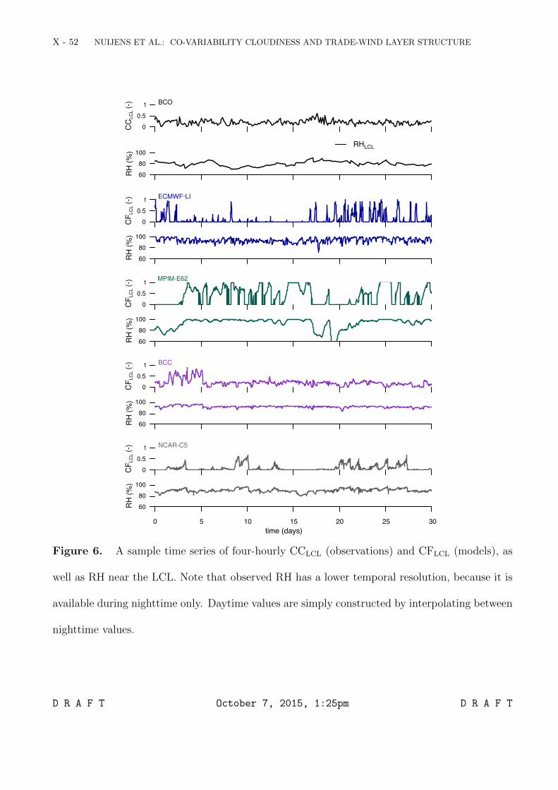
X - 52 NUIJENS ET AL.: CO-VARIABILITY CLOUDINESS AND TRADE-WIND LAYER STRUCTURE
RHLCL
0 5 10 15 20 25 30time (days)
Figure 6. A sample time series of four-hourly CCLCL (observations) and CFLCL (models), as
well as RH near the LCL. Note that observed RH has a lower temporal resolution, because it is
available during nighttime only. Daytime values are simply constructed by interpolating between
nighttime values.
D R A F T October 7, 2015, 1:25pm D R A F T

NUIJENS ET AL.: CO-VARIABILITY CLOUDINESS AND TRADE-WIND LAYER STRUCTURE X - 53
Abbreviation LCLσ2CFALOFT /σ2CFLCL
BCO 925 1.8ECMWF-LI 967 1.0MPIM-E63 941 0.2MPIM-E62 941 0.0BCC 945 1.3CCCma 911 0.03IPSL 978 0.2CNRM 904 0.5MOHC 930 0.8MRI 929 2.1NCAR-C4 930 1.0NCAR-C5 936 0.5
Table 2. The approximate level of cloud base or the LCL, taken as the level at which the
mean RH profile maximizes, restricted to levels with p > 850 hPa. Also tabulated is the ratio of
the variance in CFALOFT to CFLCL (for the models) and of the variance in CCALOFT to CCLCL
(for the observations).
a b
‘‘
Figure 7. Observed anomalous profiles of specific humidity q for 15 minute periods with large
values of cloudiness, denoted in black, and small values of cloudiness, denoted in grey. Cloudiness
is measured by CCLCL (a) and CCALOFT (b). The anomalies are taken with respect to the eight-
hourly nighttime mean q profile, of which the lower and upper quartiles are shown. Because the
observed temperature profiles only have an hourly resolution, temperature and therefore relative
humidity anomalies are not shown.
D R A F T October 7, 2015, 1:25pm D R A F T

X - 54 NUIJENS ET AL.: CO-VARIABILITY CLOUDINESS AND TRADE-WIND LAYER STRUCTURE
Abbreviation R2 (1d) Xs (1d) r2 (1d) Xm (1d) R2 (30d) Xs (30d) r2 (30d) Xm (30d)
BCO 0.24 ω825 0.10 〈RH〉ML 0.56 dθ/dzTL 0.30 UL0
ECMWF-LI 0.28 〈RH〉ML 0.21 〈RH〉ML 0.72 ω825 0.62 〈RH〉ML
MPIM-E63 0.28 〈RH〉ML 0.25 〈RH〉ML 0.62 〈RH〉ML 0.50 〈RH〉ML
MPIM-E62 0.66 〈RH〉ML 0.61 〈RH〉ML 0.80 〈RH〉ML 0.61 〈RH〉ML
BCC 0.56 〈RH〉ML 0.42 〈RH〉ML 0.72 dθ/dzTL 0.63 dθ/dzTL
CCCma 0.27 〈RH〉ML 0.13 〈RH〉ML 0.52 〈RH〉ML 0.31 〈RH〉ML
IPSL 0.02 - - - 0.12 - - -CNRM 0.44 dθ/dzTL 0.28 dθ/dzTL 0.67 dθ/dzTL 0.23 dθ/dzTL
MOHC 0.48 ω825 0.38 dθ/dzTL 0.83 dθ/dzTL 0.69 dθ/dzTL
MRI 0.30 ∆CLRH 0.15 dθ/dzTL 0.49 ∆CLRH 0.10 〈RH〉ML
NCAR-C4 0.66 dθ/dzTL 0.53 dθ/dzTL 0.75 dθ/dzTL 0.53 dθ/dzTL
NCAR-C5 0.50 〈RH〉ML 0.46 〈RH〉ML 0.67 〈RH〉ML 0.58 dθ/dzTL
Table 3. From left to right: the total fraction of variance in daily CFLCL (models) and CCLCL
(observations) explained using six parameters (see below); the parameter Xs that best explains
variance in daily CFLCL using a single regression; r2, the fraction of variance explained by Xs; the
parameter Xm that best explains variance in daily CFLCL using a multivariate regression (in which
other parameters are held constant). The following four columns show the same information for
monthly CFLCL. The parameters used are: 1) the average RH in the well-mixed layer 〈RH〉ML, 2)
the difference in RH across the cloud layer ∆CLRH, 3) the difference in RH across the inversion
layer ∆ILRH, 4) the θ lapse rate across the transition layer or mixed-layer top dθ/dzTL, 5) the
vertical velocity at 825hPa ω825 and 6) the near surface wind speed UL0.
D R A F T October 7, 2015, 1:25pm D R A F T

NUIJENS ET AL.: CO-VARIABILITY CLOUDINESS AND TRADE-WIND LAYER STRUCTURE X - 55
q
Fb
q+δqηLCL
E
w
M
1. 2. 3.
Figure 8. Illustration of the negative feedback mechanism that constrains cloud amount near
cloud base, adapted from a Figure by Neggers et al. [2006]. In 1) a typical humidity profile above
the ocean’s surface is illustrated, along with the location of the top of the well-mixed layer η,
shown by a dashed line, the lifting condensation level(s), shown as a blue shaded layer, the surface
buoyancy flux Fb,s, and the processes that control the mass budget of the well-mixed layer (see
Equation 1): the mass flux M , the entrainment rate at η, E and the large-scale vertical velocity
at η, wη. In 2) a scenario is illustrated whereby the mixed-layer q is perturbed by adding an
amount of moisture δq. This lowers the surface energy input and the LCL, which in turn increases
cloud (core) fraction and through Equation 2 increases M . M removes moisture from the well-
mixed layer and transports it upwards, thereby deepening the layer, which leads to additional
downward mixing of drier free tropospheric air. In 3) the adjustment to a new equilibrium is
shown, whereby larger M has led to a lowering of η (through Equation 1), bringing it close again
to the LCL, thereby reducing cloud (core) fraction again.
D R A F T October 7, 2015, 1:25pm D R A F T

X - 56 NUIJENS ET AL.: CO-VARIABILITY CLOUDINESS AND TRADE-WIND LAYER STRUCTURE
Figure 9. The anomalous thermodynamic and kinetic profiles for months with large CCALOFT
(observations) or CFALOFT (models) (thick lines) and small values of CCALOFT,CFALOFT (thin
lines). The top row shows the observations, and the following rows those models that frequently
produce deeper cloud layers and for which large-scale parameters explain a larger fraction of
variance in cloudiness aloft than they do in observations (R2 (30d), Table 3).
D R A F T October 7, 2015, 1:25pm D R A F T

NUIJENS ET AL.: CO-VARIABILITY CLOUDINESS AND TRADE-WIND LAYER STRUCTURE X - 57
Abbreviation R2 (1d) Xs (1d) r2 (1d) Xm (1d) R2 (30d) Xs (30d) r2 (30d) Xm (30d)
BCO 0.44 ∆CLRH 0.28 ∆CLRH 0.69 〈RH〉ML 0.42 ∆ILθECMWF-LI 0.39 ∆ILRH 0.24 ∆CLRH 0.79 ∆ILRH 0.48 UL0
MPIM-E63 0.19 ∆CLRH 0.15 ∆CLRH 0.46 ∆CLRH 0.16 ∆CLRHMPIM-E62 0.05 - - - 0.10 - - -BCC 0.54 ∆CLRH 0.31 ∆CLRH 0.76 ∆CLRH 0.49 ∆CLRHCCCma 0.11 - - - 0.47 ∆CLRH 0.32 ∆ILθIPSL 0.37 ∆ILRH 0.26 ∆CLRH 0.62 ∆ILRH 0.60 UL0
CNRM 0.45 ω825 0.35 〈RH〉ML 0.66 ω825 0.36 UL0
MOHC 0.52 ω825 0.43 ∆CLRH 0.72 ω825 0.36 ∆ILRHMRI 0.65 ω825 0.43 ∆CLRH 0.82 ∆CLRH 0.64 ∆CLRHNCAR-C4 0.58 ∆CLRH 0.29 ∆CLRH 0.80 ∆ILRH 0.48 ∆CLRHNCAR-C5 0.49 ∆CLRH 0.28 ∆CLRH 0.67 ∆CLRH 0.50 ∆CLRH
Table 4. Similar to Table 3, but then for the variance explained in CCALOFT (observations)
and CFALOFT (models). The set of parameters used is the same, with one main difference,
dθ/dz = ∆ILθ. For the observations and those models that produce clouds beyond 1 km often,
the relationship of CCALOFT,CFALOFT with dθ/dzTL is similar to that of CCLCL,CFLCL with
dθ/dzTL.
linea
r reg
ress
ion
coef
ficie
nt
Figure 10. As in Figure 5, but then for the variance explained in CFALOFT (models) and
CCALOFT (observations). The set of parameters used is the same with one main difference, ∆ILθ
is used instead of dθ/dzTL.
D R A F T October 7, 2015, 1:25pm D R A F T

X - 58 NUIJENS ET AL.: CO-VARIABILITY CLOUDINESS AND TRADE-WIND LAYER STRUCTURE
a b c
d e f
g
Figure 11. Each panel displays the difference (δ) in a parameter between days with a uniform
distribution of moisture across the cloud layer and days with a less uniform distribution of
moisture, as measured by ∆CLRH = RH850-RHLCL. δ is derived as follows: days are ordered
by ∆CLRH from high to low values. The difference between the upper and lower quartiles of
days are taken: δ ≡ φupper − φlower, whereby φupper and φlower are the average φ’s over the upper
respectively lower quartile of days. The selected parameters are: (a - g) CFALOFT, CFLCL, γ∗
(changes in the shape of the cloud profile, section 3.2), 〈RH〉ML, ∆ILθ, dθ/dzTL and ∆ILRH =
RH700 - RH850. The grey shaded box indicates negative δ’s.
D R A F T October 7, 2015, 1:25pm D R A F T
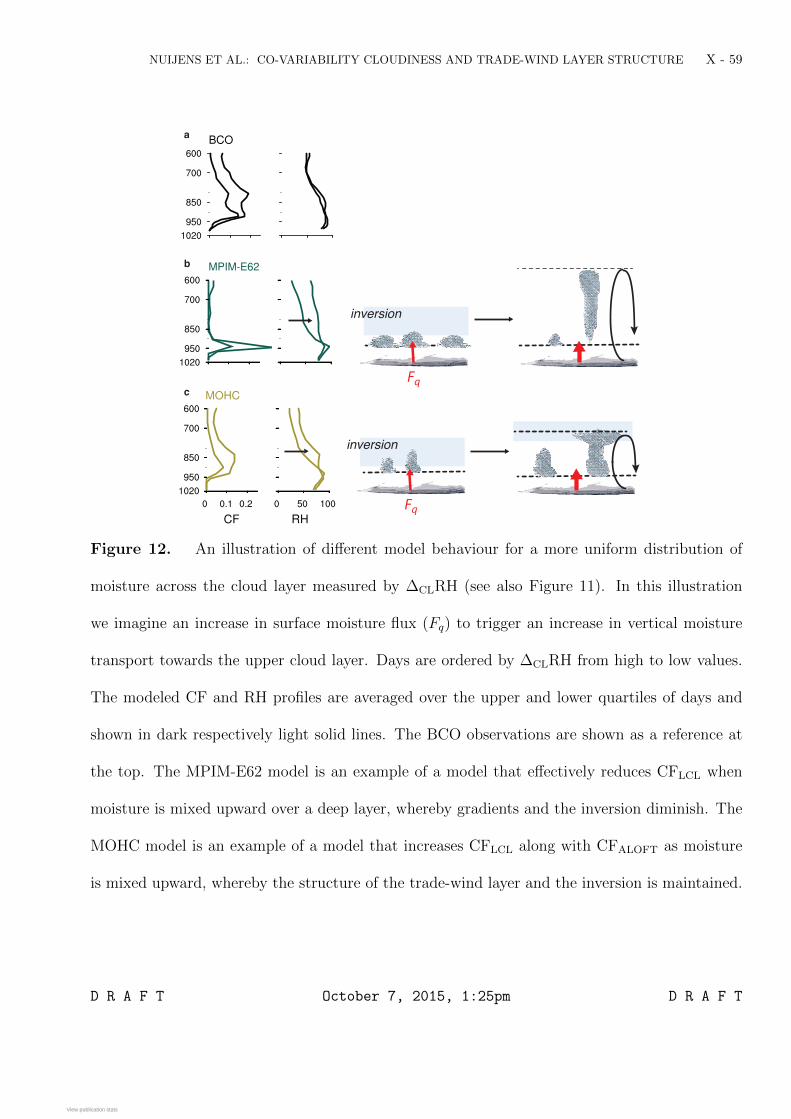
NUIJENS ET AL.: CO-VARIABILITY CLOUDINESS AND TRADE-WIND LAYER STRUCTURE X - 59
Fq
inversion
Fq
inversion
a
b
a
c
Figure 12. An illustration of different model behaviour for a more uniform distribution of
moisture across the cloud layer measured by ∆CLRH (see also Figure 11). In this illustration
we imagine an increase in surface moisture flux (Fq) to trigger an increase in vertical moisture
transport towards the upper cloud layer. Days are ordered by ∆CLRH from high to low values.
The modeled CF and RH profiles are averaged over the upper and lower quartiles of days and
shown in dark respectively light solid lines. The BCO observations are shown as a reference at
the top. The MPIM-E62 model is an example of a model that effectively reduces CFLCL when
moisture is mixed upward over a deep layer, whereby gradients and the inversion diminish. The
MOHC model is an example of a model that increases CFLCL along with CFALOFT as moisture
is mixed upward, whereby the structure of the trade-wind layer and the inversion is maintained.
D R A F T October 7, 2015, 1:25pm D R A F T
View publication statsView publication stats