RESEARCH ARTICLE10.1002/2015JC010788

Observations and model simulations of wave-currentinteraction on the inner shelfJulia Hopkins1, Steve Elgar2, and Britt Raubenheimer2

1MIT-WHOI Joint Program in Civil and Environmental Engineering, Cambridge, Massachusetts, USA, 2Woods HoleOceanographic Institution, Woods Hole, Massachusetts, USA

Abstract Wave directions and mean currents observed for two 1 month long periods in 7 and 2 m waterdepths along 11 km of the southern shoreline of Martha’s Vineyard, MA, have strong tidal modulations.Wave directions are modulated by as much as 708 over a tidal cycle. The magnitude of the tidal modulationsin the wavefield decreases alongshore to the west, consistent with the observed decrease in tidal currentsfrom 2.1 to 0.2 m/s along the shoreline. A numerical model (SWAN and Deflt3D-FLOW) simulating wavesand currents reproduces the observations accurately. Model simulations with and without wave-currentinteraction and tidal depth changes demonstrate that the observed tidal modulations of the wavefieldprimarily are caused by wave-current interaction and not by tidal changes to water depths over the nearbycomplex shoals.

1. Introduction

Understanding wave propagation across the continental shelf to the shore is critical to predicting forces onshoreline structures, increases in wave-driven water levels, wave overtopping and flooding, dangerouswave-driven surfzone currents, sediment transport, and beach erosion and accretion. As waves propagate(shoal) over increasingly shallow bathymetry, conservation of energy flux causes wave heights to becomelarger before breaking. Breaking waves dissipate energy while transferring momentum flux to the water col-umn. In the surf zone, the time-averaged wave-driven forcing raises water levels near the shoreline[Longuet-Higgins and Stewart, 1964], producing alongshore varying sea levels and currents [Apotsos et al.,2008; Shi et al., 2011; Hansen et al., 2015] and, in the case of obliquely incident waves, driving alongshorecurrents in the direction of wave propagation [Longuet-Higgins, 1970; Thornton and Guza, 1986; Guza et al.,1986; Feddersen et al., 1998; and many others]. The wave-orbital velocities and wave-generated currents cantransport sediment and act as a mechanism for shoreline evolution [Fredsoe and Deigaard, 1992; van Rijn,1993; Amoudry and Souza, 2011; references therein; and many others].

The energy and direction of waves propagating across the continental shelf to the shore are affected by thebathymetry and by currents, both of which cause shoaling and refraction. Wave energy can be increased byshoaling and decreased by dissipative processes, including bottom friction, whitecapping, and depth-limited breaking. Depth-induced refraction increases with decreasing wave frequency and redirects wavecrests to align with bathymetry in shallow water (potentially resulting in areas with wave focusing and shad-owing), although breaking waves are not necessarily normally incident. Similarly, currents change waveheight and direction by altering the wave number k, given by the linear dispersion relationship:

r5ffiffiffiffiffiffiffiffiffiffiffiffiffiffiffiffiffiffiffiffiffiffiffiffigktanh ðkhÞ

p(1)

where r is the intrinsic wave frequency, g is the gravitational acceleration, and h is the water depth. A cur-rent U interacting with the wavefield causes the intrinsic frequency to be Doppler shifted such that theapparent (e.g., observed) frequency x becomes [Longuet-Higgins and Stewart, 1961; Wolf and Prandle, 1999]:

x5r1k � U (2)

which, by reapplication of (1) to the Doppler-shifted frequency x in place of r, gives a new wave number.Changes in wave number cause changes to energy flux, ECg, where E is energy and Cg 5 F(x, k) is the groupvelocity. Changes in wave number likewise affect wave direction, h. Similar to depth-induced changes,

Key Points:� Observed large tidal modulations to

the wavefield on the inner shelf� SWAN1Delft3D-FLOW model

simulates observations accurately� Model shows modulations are owing

to wave-current interaction notdepth changes

Correspondence to:J. Hopkins,hychenj@mit.edu

Citation:Hopkins, J., S. Elgar, andB. Raubenheimer (2016), Observationsand model simulations of wave-current interaction on the inner shelf,J. Geophys. Res. Oceans, 121, 198–208,doi:10.1002/2015JC010788.

Received 17 FEB 2015

Accepted 4 DEC 2015

Accepted article online 13 DEC 2015

Published online 10 JAN 2016

VC 2015. American Geophysical Union.

All Rights Reserved.

HOPKINS ET AL. 198

Journal of Geophysical Research: Oceans

PUBLICATIONS

current-induced changes in h (relative to the current direction) between two locations (A and B) are givenby Snell’s Law:

kAsinðhAÞ5kBsinðhBÞ (3)

There have been many investigations of current-induced wave height growth or decay, usually for the caseof currents flowing in the same or opposite direction of the waves [Gonzalez, 1984; Jonsson, 1990; Wolf andPrandle, 1999; Olabarrieta et al., 2011, 2014; Elias et al., 2012; and many others]. There are fewer observatio-nal studies of the current-induced changes in wave direction, partially because waves propagating into anopposing or following current (h 5 08 or 1808), such as commonly occurs near strong jets from inlets, rivermouths, and estuaries, do not change direction (equation (3)). The change in direction is maximum forangles near h 5 458, and increases with current speed and wave frequency (equations (1–3)) [Wolf andPrandle, 1999].

Tidal modulations of 6108 have been observed in 12–18 m water depth for relatively high-frequency (0.5Hz) waves [Wolf and Prandle, 1999] and in 11 m depth for swell-dominated (0.05–0.30 Hz) wavefields [Han-sen et al., 2013]. It was hypothesized that the modulation of the high-frequency wave direction was owingto tidal currents [Wolf and Prandle, 1999], and numerical simulations of one tidal cycle suggest the direc-tional changes in the observed swell wavefield likewise were owing to currents, not to tidal changes inwater depth [Hansen et al., 2013]. Here tidally modulated changes to wave heights and directions in 7 and2 m water depths along an Atlantic Ocean shoreline are investigated with both observations from two 1month long periods and numerical model simulations.

2. Methods

2.1. Field ObservationsWater levels, waves, and currents were measured for approximately 1 month along 11 km of the southernshoreline of Martha’s Vineyard, MA, (Figure 1) in both August 2013 and July–August 2014. In 2013 and 2014,along the 7 m depth isobath, 1 min mean current profiles in 0.5 m high vertical bins between 0.5 m abovethe seafloor and the sea surface were obtained with Nortek 1 MHz AWAC acoustic Doppler current profilersfor 12 min every half hour, followed by 1024 s of 2 Hz samples of bottom pressure, sea-surface elevation

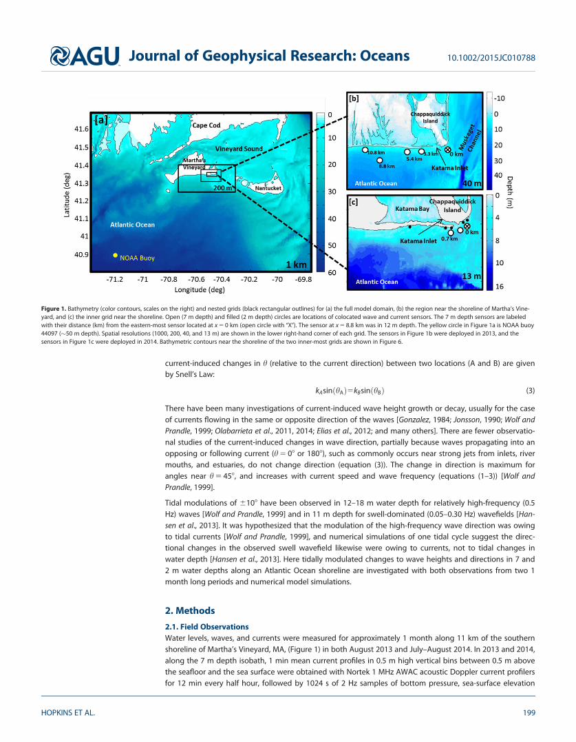
Figure 1. Bathymetry (color contours, scales on the right) and nested grids (black rectangular outlines) for (a) the full model domain, (b) the region near the shoreline of Martha’s Vine-yard, and (c) the inner grid near the shoreline. Open (7 m depth) and filled (2 m depth) circles are locations of colocated wave and current sensors. The 7 m depth sensors are labeledwith their distance (km) from the eastern-most sensor located at x 5 0 km (open circle with ‘‘X’’). The sensor at x 5 8.8 km was in 12 m depth. The yellow circle in Figure 1a is NOAA buoy44097 (�50 m depth). Spatial resolutions (1000, 200, 40, and 13 m) are shown in the lower right-hand corner of each grid. The sensors in Figure 1b were deployed in 2013, and thesensors in Figure 1c were deployed in 2014. Bathymetric contours near the shoreline of the two inner-most grids are shown in Figure 6.

Journal of Geophysical Research: Oceans 10.1002/2015JC010788

HOPKINS ET AL. 199

(from a 1 MHz vertical acoustic beam), and near-surface velocities to estimate wave characteristics. In 2013,an additional sensor was deployed in 12 m depth (Figure 1b), 8.8 km west of the eastern-most sensorlocated at x 5 0 km. In 2014, 2 Hz observations of currents (0.8 m above the seafloor) and near-bottom pres-sure were measured with 10 MHz Sontek Triton acoustic Doppler velocimeters at five locations along the2 m depth isobath from x 5 0 to x 5 3.3 km (Figure 1c).

There was little vertical structure to the mean currents in 7 and 12 m depth except in the bottom and top0.5 m high bins, so the interior bins were used to estimate depth-averaged flows. The two 12 min profilingperiods every hour were combined to provide estimates of 1 h means of the depth-averaged currents. Onehour averages of the alongshore component of the single-point velocity measurements in 2 m depth areassumed to be representative of depth-averaged alongshore flows. The 2 Hz time series were used to esti-mate significant wave heights (Hsig, 4 times the standard deviation of sea-surface fluctuations) and wavedirections [Kuik et al., 1988] in the frequency (f) band 0.05< f< 0.30 Hz. Bottom pressures were convertedto sea-surface elevation using linear wave theory.

The bathymetry in the region is complex (Figure 1), including islands, shoals, and the rapidly migratingKatama Inlet [Ogden, 1974] that separates Katama Bay from the Atlantic Ocean. Bathymetric surveys of theshoreline, inlet channel, and ebb shoal near Katama Inlet were performed in summer 2013 and 2014 with aGPS and an acoustic altimeter mounted on a jetski. The horizontal resolution of the jetski surveys is on theorder of 10 m, with finer resolution near steep features. Additional bathymetry was obtained during 1998and 2008 USGS surveys (Northeast Atlantic 3 arc second map, National Geophysical Data Center [1999] andNantucket 1/3 arc second map, Eakins et al. [2009]), and has horizontal resolution of 10–90 m. The southernshoreline of Martha’s Vineyard is oriented east-west (Figure 1). West of Katama Inlet, bathymetry contours,especially in depths less than �10 m are roughly parallel to the shoreline (Figure 1b). However, south andeast of Katama Inlet and Bay, the bathymetry is cross-shore and alongshore inhomogeneous.

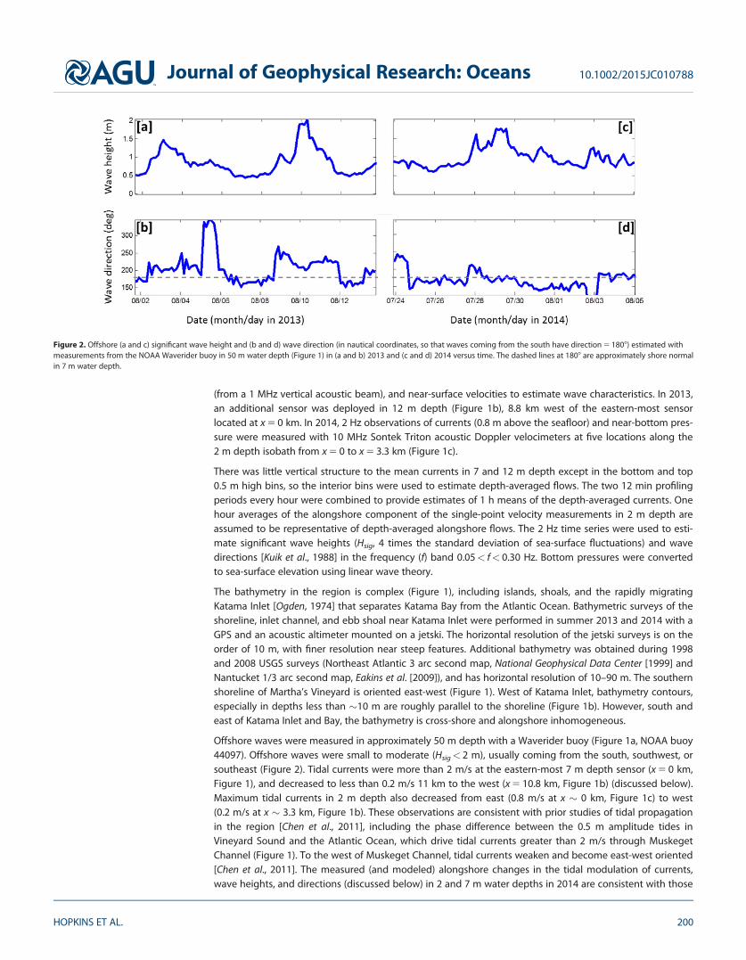
Offshore waves were measured in approximately 50 m depth with a Waverider buoy (Figure 1a, NOAA buoy44097). Offshore waves were small to moderate (Hsig< 2 m), usually coming from the south, southwest, orsoutheast (Figure 2). Tidal currents were more than 2 m/s at the eastern-most 7 m depth sensor (x 5 0 km,Figure 1), and decreased to less than 0.2 m/s 11 km to the west (x 5 10.8 km, Figure 1b) (discussed below).Maximum tidal currents in 2 m depth also decreased from east (0.8 m/s at x � 0 km, Figure 1c) to west(0.2 m/s at x � 3.3 km, Figure 1b). These observations are consistent with prior studies of tidal propagationin the region [Chen et al., 2011], including the phase difference between the 0.5 m amplitude tides inVineyard Sound and the Atlantic Ocean, which drive tidal currents greater than 2 m/s through MuskegetChannel (Figure 1). To the west of Muskeget Channel, tidal currents weaken and become east-west oriented[Chen et al., 2011]. The measured (and modeled) alongshore changes in the tidal modulation of currents,wave heights, and directions (discussed below) in 2 and 7 m water depths in 2014 are consistent with those

Figure 2. Offshore (a and c) significant wave height and (b and d) wave direction (in nautical coordinates, so that waves coming from the south have direction 5 1808) estimated withmeasurements from the NOAA Waverider buoy in 50 m water depth (Figure 1) in (a and b) 2013 and (c and d) 2014 versus time. The dashed lines at 1808 are approximately shore normalin 7 m water depth.

Journal of Geophysical Research: Oceans 10.1002/2015JC010788

HOPKINS ET AL. 200

in 7 m depth in 2013, suggesting that the westward decrease in tidal modulation is owing to a temporallyconstant spatial structure, not a change in behavior from 2013 to 2014.

2.2. Numerical ModelA coupled wave and flow numerical model was used to investigate the processes leading to the spatial andtemporal structure of the waves and currents observed south of Martha’s Vineyard. Waves were modeledwith SWAN [Booij et al., 1999] by solving the wave action conservation equation, and currents were mod-eled with Delft3D-FLOW [Lesser et al., 2004] by solving the nonlinear shallow water equations. The wavemodel includes depth-induced and current-induced refraction, and dissipation owing to whitecapping,depth-induced breaking, and bottom friction. Wind was not implemented because observed winds usuallywere less than 5 m/s (mean (standard deviation) were 2.8 (1.6) and 3.4 (2.0) m/s in 2013 and 2014, respec-tively). For the conditions observed here, model results with wind were not significantly different thanresults without wind. Quartet and triad nonlinear interactions were turned off owing to the lack of windforcing, the relatively short propagation distances in deep water, and the focus on observations seaward ofthe region of strong quadratic nonlinearities (where kh� 1). Although quadratic nonlinear interactions areimportant to many aspects of wave evolution in shallow water [Freilich and Guza, 1984], their effects onbulk (energy weighted) statistics of the wavefield (e.g., wave height, average direction, centroidal fre-quency) are relatively small [Gorrell et al., 2011]. The circulation model includes the effects of waves on cur-rents through wave radiation-stress gradients, combined wave and current bed shear stress, and Stokesdrift. The wave and flow models were coupled, such that FLOW passes water levels and Eulerian depth-averaged velocities to SWAN, and SWAN passes wave parameters to FLOW, which is run continuously for�0.25 s time intervals. Similar combined wave and circulation models have been used to investigate wave-current interactions on the inner shelf (8–15 m depth) [Hansen et al., 2013], in the surf zone [Hansen et al.,2014, 2015; Chen et al., 2015], near river mouths [Elias et al., 2012], and in coastal bays [Mulligan et al., 2010].

SWAN and Delft3D-FLOW (in depth-averaged mode) were run over 3 (2013) and 4 (2014) nested grids (Fig-ure 1a) with both two-way (FLOW) and one-way nesting (SWAN). The outermost grid, with 1 km resolution,spans about 150 km along the north and south boundaries and 100 km along the east and west boundaries.Nested in this coarse grid are finer grids of 200 and 40 m resolution in 2013, and a third grid with 13 m reso-lution in 2014 to compare with the closely spaced observations (0� x� 0.7 km, Figure 1c) obtained in 2014.Nesting allows calculations on the coarser grids to serve as boundary conditions for the finer grids, enhanc-ing the resolution of the model near the shoreline with minimal computational cost. The combined USGSlarge-scale and either the 2013 or the 2014 high-resolution shoreline bathymetry were interpolated ontoeach of the nested grids.

SWAN has skill in a range of environments, including the inner shelf south of Martha’s Vineyard (12–27 mdepth) [Ganju and Sherwood, 2010; Ganju et al., 2011] and many shallow water areas [Magne et al., 2007;Mulligan et al., 2010], whether forced with observations [Gorrell et al., 2011; Chen et al., 2015; Hansen et al.,2013, 2014, 2015] or with output from global wave models [van der Westhuysen, 2010; Kumar et al., 2012].Here, SWAN was run in stationary mode, with wavefield boundary conditions supplied every 3 h. Stationarymode solves for equilibrium wave conditions for a given set of boundary conditions and is less computa-tionally expensive than nonstationary mode. For the 3 h periods and for the wind and wave conditionsused here, the assumption of stationarity is not violated even for the largest grid. For the 2013 bathymetry,boundary conditions were a JONSWAP frequency-directional (cosN(h), where the default value of N 5 20was used) spectrum based on the mean wave direction h, Hsig, and average wave period provided by themodel WaveWatchIII (WWIII) [Tolman, 2002] every 3 km along the open (water) boundaries of the outergrid. The wave model also was run using the frequency-directional spectrum estimated with observationsat the buoy in 50 m water depth (Figure 1a) applied uniformly at each point on the boundaries of the outergrid. For southerly waves (which are the most common), model skill was similar for the spatially variableWWIII wave forcing and the spatially uniform buoy forcing. However, model skill was significantly higherwith the spatially varying WWIII boundary conditions than with the spatially constant buoy conditions whenwaves at the buoy came from the north or northeast, in which case the spatially varying wavefield is notrepresented well by the measurements near the southwest corner of the domain (Figure 1a). WWIII simula-tions were not available in 2014, so buoy observations were used on the boundaries (wave conditions weresoutherly). In all cases, SWAN solves the spectral action balance using 36 directional bins (108/bin) and 37frequency bands logarithmically spaced between 0.03 and 1.00 Hz. The wave model used a depth-limited

Journal of Geophysical Research: Oceans 10.1002/2015JC010788

HOPKINS ET AL. 201

wave breaking formulation without rollers [Battjes and Janssen, 1978] with the default value c 5 Hsig/h 5 0.73, and a JONSWAP bottom friction coefficient associated with wave-orbital motions set higher(0.100 m2/s3) than the default (0.067 m2/s3) [Hasselmann et al., 1973]. The higher coefficient resulted inmore accurate modeled wave heights. Using default coefficients, observed wave heights were under pre-dicted using some friction formulations [Madsen et al., 1988] and over predicted using other approaches[Collins, 1972]. Model wave directions were insensitive to the friction formulation.

The circulation model Deflt3D-FLOW solves the time-varying nonlinear shallow water equations on a stag-gered Arakawa-C grid using an alternating-direction-implicit solver [Lesser et al., 2004] to compute currentsthroughout the modal domain. The model was run using the 13 most energetic satellite-generated tidalconstituents [Egbert and Erofeeva, 2002] along open boundaries, which were dominated by the M2 (�80%of the variance, with small changes depending on location along the boundary) and N2 (�10% of the var-iance) constituents. In addition, the model used a free slip condition at closed (land) side boundaries, a spa-tially uniform Chezy roughness of 65 m0.5/s (roughly equivalent to a drag coefficient of Cd 5 0.0023) atbottom boundaries, and default Delft3D parameters for coupling the FLOW and WAVE models [Deltares,2014]. Second-order differences were used with a time step of 0.25 s for 2013 (40 m spacing in the highestresolution grid) and 0.15 s for 2014 (13 m spacing) for numerical stability.

Model parameters (e.g., time steps, grid resolution) were chosen to accommodate future studies of shore-line evolution in the Katama region on time scales varying from that of individual storms to seasons toyears. Spatial and temporal resolutions are fine enough for numerical stability and verification with observa-tions. Using higher resolution does not change simulation results significantly and requires more computa-tional effort.

3. Results

Model predictions of the sea levels, waves, and currents are comparable with observations in 7 and 2 mwater depths in the area south of Martha’s Vineyard. The model simulates the observed 3 h sea level fluctu-ations (primarily the M2 tide) fairly well (within a few cm), although occasionally it underpredicts the min-ima and maxima by as much as 0.10–0.15 m (Figure 3). These model-data differences could be owing toimperfect tidal boundary conditions, inaccurate model bathymetry, or unmodeled physical processes. Simi-lar to previous results [van der Westhuysen, 2010; Mulligan et al., 2010; Gorrell et al., 2011; Hansen et al., 2015;and many others], the model skillfully predicts the wave heights observed in 7 (Figures 4a–4c) and 2 m(Figures 5a and 5b) depth. Model-data wave height discrepancies in shallow water (e.g., Figure 5b) could becaused by inaccurate model bottom friction, incorrect model simulations of sea level, or inaccurate modelbathymetry. The small errors in wave height (which typically are over estimated at all tide levels) are morelikely owing to inaccurate bathymetry than to the under estimation of the range of sea level fluctuations.The model also skillfully predicts the wave directions (Figures 4d–4f and 5c, 5d), including the large tidalmodulations observed near the eastern edge of the domain (x 5 0.3 km, Figure 4f).

Figure 3. Observed (black curves) and modeled (red curves) 3 h average sea-surface elevations (relative to mean sea level) versus time at locations (Figure 1b) x 5 (a) 10.8, (b) 3.3, and(c) 0.3 km (distances are relative to the sensor at x 5 0 km). RMSE values (normalized by the data range) are given in the lower left-hand corners.

Journal of Geophysical Research: Oceans 10.1002/2015JC010788

HOPKINS ET AL. 202

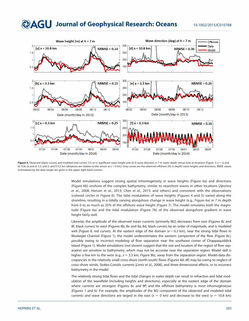
Model simulations suggest strong spatial inhomogeneity in wave heights (Figure 6a) and directions(Figure 6b) onshore of the complex bathymetry, similar to nearshore waves in other locations [Apotsoset al., 2008; Hansen et al., 2013; Chen et al., 2015; and others] and consistent with the observations(colored circles in Figure 6). The tidal modulation of wave heights (Figures 4 and 5) varied along theshoreline, resulting in a tidally varying alongshore change in wave height (e.g., Figure 6a) in 7 m depthfrom 0 to as much as 35% of the offshore wave height (Figure 7). The model simulates both the magni-tude (Figure 6a) and the tidal modulation (Figure 7b) of the observed alongshore gradient in waveheight fairly well.

Likewise, the amplitude of the observed mean currents (primarily M2) decreases from east (Figures 8c and8f, black curves) to west (Figures 8b, 8e and 8a, 8d, black curves) by an order of magnitude, and is modeledwell (Figure 8, red curves). At the eastern edge of the domain (x 5 0.3 km), near the strong tidal flows inMuskeget Channel (Figure 1), the model underestimates the western component of the flow (Figure 8c),possibly owing to incorrect modeling of flow separation near the southeast corner of ChappaquiddickIsland (Figure 1). Model simulations (not shown) suggest that the size and location of the region of flow sep-aration are sensitive to bathymetry, which may not be accurate near the separation region. Model skill ishigher a few km to the west (e.g., x 5 3.3 km, Figure 8b), away from the separation region. Model-data dis-crepancies in the relatively small cross-shore (north-south) flows (Figures 8d–8f) may be owing to neglect ofcross-shore winds, Stokes-Coriolis currents [Lentz et al., 2008], and three-dimensional effects, or to incorrectbathymetry in the model.

The relatively strong tidal flows and the tidal changes in water depth can result in refraction and tidal mod-ulation of the wavefield (including heights and directions), especially at the eastern edge of the domainwhere currents are strongest (Figures 8c and 8f) and the offshore bathymetry is most inhomogeneous(Figures 1 and 6). For example, the amplitudes of the M2 component of the observed and modeled tidalcurrents and wave directions are largest in the east (x 5 0 km) and decrease to the west (x 5 10.8 km)

Figure 4. Observed (black curves) and modeled (red curves) 3 h (a–c) significant wave height and (d–f) wave direction in 7 m water depth versus time at locations (Figure 1) x 5 (a andd) 10.8, (b and e) 3.3, and (c and f) 0.3 km (distances are relative to the sensor at x 5 0 km). Gray curves are the observed offshore (50 m depth) wave heights and directions. RMSE values(normalized by the data range) are given in the upper right-hand corners.

Journal of Geophysical Research: Oceans 10.1002/2015JC010788

HOPKINS ET AL. 203

(Figure 9). Near the eastern edge of the domain (x< 0.5 km, Figure 9), the model under predicts the M2amplitudes of the mean currents (Figures 8c and 9) and the wave directions, possibly because horizontalflow separation around Chappaquiddick Island becomes important in this region. Additionally, small errorsin the amplitude of tidal boundary conditions could contribute to mismatch between simulated andobserved current and wave direction M2 amplitudes.

Figure 5. Observed (black curves) and modeled (red curves) 3 h (a and b) significant wave height and (c and d) wave direction in 2 m water depth versus time at locations (Figure 1)x 5 (a and c) 0.8 and (b and d) 0 km (distances are relative to the sensor at x 5 0 km). Gray curves are the observed offshore (50 m depth) wave heights and directions. RMSE values(normalized by the data range) are given in the upper right-hand corners.

Figure 6. Spatial distribution (color contours, scales on the right) of modeled (a) significant wave height and (b) wave direction on 3 August 2013 09:00 h EDT during flood tide (flowfrom west to east into Muskeget Channel). Black curves are depth contours every 5 m, and the black circles are filled with the color of the observed values at those locations. If modeland data agree, the color inside the circle matches the color of the surrounding model contours.

Journal of Geophysical Research: Oceans 10.1002/2015JC010788

HOPKINS ET AL. 204

To determine if the M2 fluctuations in the wavefield are caused by depth-induced or current-inducedrefraction or both, the model was run with both currents and tidal depth oscillations, with tidal depth oscil-lations, but no currents, and with currents, but no tidal depth oscillations. The observed tidal fluctuationsin the alongshore gradient of wave heights are simulated better by the model with currents and depthchanges (compare the blue with the black curve in Figure 7b) than by the model with depth changes only(Figure 7b, red curve). The modeled gradients with currents, but no depth changes (Figure 7b, green curve)are similar to those using the full model (currents and depth changes, Figure 7b, blue curve), suggestingthe modulations of the alongshore gradients in wave heights primarily are caused by current-inducedrefraction.

Figure 7. (a) Difference between the significant wave height observed in 7 m depth at x 5 3.3 km and at x 5 10.8 km versus time. (b) Energy density of the time series of alongshore dif-ference in wave height versus frequency for observations (black curve) and simulated by the model including tidal currents and water depth changes (blue curve), currents, but no depthchanges (green curve), and depth changes, but no currents (red curve). The spectra have 36 degrees of freedom, and the 95% confidence levels are shown.

Figure 8. Observed (black curves) and modeled (red curves) 1 h mean depth-averaged (a–c) east and (d–f) north velocity in 7 m water depth versus time at locations (Figure 1) x 5 (aand b) 10.8, (c and d) 3.3, and (e and f) 0.3 km. RMSE values (normalized by the data range) are given in the upper right-hand corners.

Journal of Geophysical Research: Oceans 10.1002/2015JC010788

HOPKINS ET AL. 205

Model tests and equations (1–3) suggest that the observed tidal modulation in wave direction also is owingto currents and not depth changes. For 0.1 Hz waves propagating from 50 to 7 m depth across tidally vary-ing currents with similar magnitudes to observed flows in Muskeget Channel, equations (1–3) predict large(6�358) modulations to the wave direction, comparable with the observations (Figures 4e, 4f, 5c, 5d, and 9)and with the model simulations that account for a frequency-directional spectrum and spatially varying cur-rents and bathymetry (Figure 10, blue curves). In contrast, the observed tidal modulations of wave directionare not reproduced by the model when currents are not included (Figure 10, red curves), but are repro-duced for the model with currents, but no tidal depth changes (Figure 10, green curves). Similar to previousmodel runs for one tidal cycle [Hansen et al., 2013], the simulations suggest that the observed tidal modula-tions of wave direction are caused primarily by current-induced refraction. As waves refract over thebathymetry between 7 and 2 m depth, the tidal modulation of direction is reduced to about 6108 relativeto shore-normal (Figures 5c and 5d). Consequently, alongshore currents (and associated sediment flux)driven by breaking waves may change direction (or strengthen and weaken) with the tide, even when off-shore wave conditions are constant.

Figure 9. Amplitude of the observed (black symbols) and modeled (red curves) tidal (M2) modulation of wave direction (open circles,dashed curve) and velocity magnitude (open diamonds, solid curve) in 7 m depth versus distance from the eastern-most sensor (x 5 0 km,Figure 1). 95% confidence intervals of the M2 amplitude estimates, calculated using a tidal frequency analysis of the time series (‘‘T_TIDE’’)[Pawlowicz et al., 2002] are shown for the observations. Some of the error bars for the observed velocity magnitude are smaller than thediamond symbols. The errors in estimating model amplitudes (not shown) are similar to those from the observations.

Figure 10. (a) Wave direction versus time at x 5 0.3 km and (b) energy density of the time series of wave direction versus frequency for observations (Figure 10b only, black curve) andsimulated by the model including tidal currents and water depth changes (blue curves), currents, but no depth changes (green curves), and depth changes, but no tidal currents (redcurves). The spectra have 36 degrees of freedom, and the 95% confidence levels are shown. Model-data time series comparisons are given in Figure 4f.

Journal of Geophysical Research: Oceans 10.1002/2015JC010788

HOPKINS ET AL. 206

4. Conclusions

A combined wave (SWAN) and circulation (Delft3D-FLOW) numerical model accurately simulates waves andcurrents observed in 7 and 2 m water depths near Katama Bay and Inlet, on the southern shoreline of Mar-tha’s Vineyard, MA in the presence of strong (>2 m/s) tidal currents and complex bathymetry. The modelreproduces the alongshore gradients in waves and mean currents, as well as the large (6358) tidal modula-tion of wave directions observed for two 1 month long periods. Model simulations with and without wave-current interactions demonstrate that the modulations of the wavefield primarily are owing to current-induced refraction, and not to tidal changes in water levels. The comparisons with observations suggestthat the model with wave-current interaction and with the parameters used here simulates waves and cur-rents accurately in regions with complex bathymetry and strong currents. These results further suggest thattidal modulations in wave direction in other coastal environments with complex bathymetry and strong cur-rents also could be owing to wave-current interaction.

ReferencesAmoudry, L. O., and A. J. Souza (2011), Deterministic coastal morphological and sediment transport modeling: A review and discussion,

Rev. Geophys., 49, RG2002, doi:10.1029/2010RG000341.Apotsos, A., B. Raubenheimer, S. Elgar, and R. T. Guza (2008), Wave-driven setup and alongshore flows observed onshore of a submarine

canyon, J. Geophys. Res., 113, C07025, doi:10.1029/2007JC004514.Battjes, J. A., and J. P. M. Janssen (1978), Energy loss and set-up due to breaking of random waves, in Proceedings of the 16th International

Conference on Coastal Engineering, 569 pp., ASCE, N. Y.Booij, N., R. C. Ris, and L. H. Holthuijsen (1999), A third-generation wave model for coastal regions: 1. Model description and validation,

J. Geophys. Res., 104(C4), 7649–7666, doi:10.1029/98JC02622.Chen, C., H. Huang, R. C. Beardsley, Q. Xu, R. Limeburner, G. W. Cowles, and H. Lin (2011), Tidal dynamics in the Gulf of Maine and New

England Shelf: An application of FVCOM, J. Geophys. Res., 116, C12010, doi:10.1029/2011JC007054.Chen, J.-L., T. J. Hsu, F. Shi, B. Raubenheimer, and S. Elgar (2015), Hydrodynamics and sediment transport modeling of New River Inlet (NC)

under the interaction of tides and waves, J. Geophys. Res. Oceans, 120, 4028–4047, doi:10.1002/2014JC010425.Collins, J. I. (1972), Prediction of shallow-water spectra, J. Geophys. Res., 77(15), 2693–2707, doi:10.1029/JC077i015p02693.Deltares, (2014), Delft3D-Wave: Simulation of Short Crested Waves With SWAN, User Manual, Deltares, Delft, Netherlands.Eakins, B. W., L. A. Taylor, K. S. Carignan, R. R. Warnken, E. Lim, and P. R. Medley (2009). Digital elevation model of Nantucket, Massachusetts:

Procedures, data sources and analysis, NOAA Tech. Memo. NESDIS NGDC-26, 29 pp., Dep. of Commerce, Boulder, Colo.Egbert, G. D., and S. Y. Erofeeva (2002), Efficient inverse modeling of barotropic ocean tides, J. Atmos. Oceanic Technol., 19, 183–204.Elias, E. P. L., G. Gelfenbaum, and A. J. Van der Westhuysen (2012), Validation of a coupled wave-flow model in a high-energy setting: The

mouth of the Columbia River, J. Geophys. Res., 117, C09011, doi:10.1029/2012JC008105.Feddersen, F., R. T. Guza, S. Elgar, and T. H. C. Herbers (1998), Alongshore momentum balances in the nearshore, J. Geophys. Res., 103(C8),

15,667–15,676, doi:10.1029/98JC01270.Fredsoe, J., and R. Deigaard (1992), Mechanics of Coastal Sediment Transport, World Sci. Publ., Singapore.Freilich, M. H., and R. T. Guza (1984), Nonlinear effects on shoaling surface gravity waves, Philos. Trans. R. Soc. London Ser. A, 311, 1–41.Ganju, N. K., and C. R. Sherwood (2010), Effect of roughness formulation on the performance of a coupled wave, hydrodynamic, and sedi-

ment transport model, Ocean Modell., 33(3–4), 299–313, doi:10.1016/j.ocemod.2010.03.003.Ganju, N. K., S. J. Lentz, A. R. Kirincich, and J. T. Farrar (2011), Complex mean circulation over the inner shelf south of Martha’s Vineyard

revealed by observations and a high-resolution model, J. Geophys. Res., 116, C10036, doi:10.1029/2011JC007035.Gonzalez, F. I. (1984), A case study of wave-current-bathymetry interactions at the Columbia River Entrance, J. Phys. Oceanogr., 14,

1065–1078.Gorrell, L., B. Raubenheimer, S. Elgar, and R. T. Guza (2011), SWAN predictions of waves observed in shallow water onshore of complex

bathymetry, Coastal Eng., 58(6), 510–516, doi:10.1016/j.coastaleng.2011.01.013.Guza, R. T., E. B. Thornton, and N. Christensen Jr. (1986), Observations of steady longshore currents in the surf zone, J. Phys. Oceanogr., 16,

1959–1969.Hansen, J. E., E. Elias, J. H. List, L. H. Erikson, and P. L. Barnard (2013), Tidally influenced alongshore circulation at an inlet-adjacent shoreline.

Cont. Shelf Res., 56, 26–38, doi:10.1016/j.csr.2013.01.017.Hansen, J. E., T. T. Janssen, B. Raubenheimer, F. Shi, P. L. Barnard, and I. S. Jones (2014), Observations of surfzone alongshore pressure gra-

dients onshore of an ebb-tidal delta, Coastal Eng., 91, 251–260, doi:10.1016/j.coastaleng.2014.05.010.Hansen, J., B. Raubenheimer, J. List, and S. Elgar (2015), Modeled alongshore circulation and force balances onshore of a submarine can-

yon, J. Geophys. Res. Oceans, 120, 1887–1903, doi:10.1002/2014JC010555.Hasselmann, K., et al. (1973), Measurements of Wind-Wave Growth and Swell Decay During the Joint North Sea Wave Project (JONSWAP),

Dtsch. Hydrogr. Z. Suppl., 8(12), 1–95.Jonsson, I. G. (1990), Wave–current interactions, in Ocean Engineering Science: The Sea, vol. 9A, edited by B. Le M�ehaut�e and D. M. Hanes,

pp. 65–120, Harvard Univ. Press, Cambridge, Mass.Kuik, A. J., G. P. van Vledder, and L. H. Holthuijsen (1988), A method for the routine analysis of pitch-and-roll buoy wave data, J. Phys. Oce-

anogr., 18, 1020–1034.Kumar, N., G. Voulgaris, J. C. Warner, and M. Olabarrieta (2012), Implementation of the vortex force formalism in the coupled ocean-

atmosphere-wave-sediment transport (COAWST) modeling system for inner shelf and surf zone applications, Ocean Modell., 47, 65–95,doi:10.1016/j.ocemod.2012.01.003.

Lentz, S., M. Fewings, P. Howd, J. Fredericks, and K. Hathaway (2008), Observations and a model of undertow over the inner continentalshelf, J. Phys. Oceanogr., 38(11), 2341–2357, doi:10.1175/2008JPO3986.1.

Lesser, G. R., J. A. Roelvink, J. A. T. M. van Kester, and G. S. Stelling (2004), Development and validation of a three-dimensional morphologi-cal model, Coastal Eng., 51, 883–915, doi:10.1016/j.coastaleng.2004.07.014.

AcknowledgmentsThe data used in this study areavailable by contacting the authors,hychenj@mit.edu or elgar@whoi.edu.Support was provided by ONR, NSF,Sea Grant, NDSEG, an MIT PresidentialGraduate Fellowship, and ASD(R&E).Mumen Alzubi, Kohl Brinkman, DanikForsman, Janet Fredericks, Levi Gorrell,Liliana Montoya, Mara Orescanin,Maddie Smith, Anna Wargula, and BillyWells helped obtain the observations,and Jeff Hansen provided valuablehelp with modeling.

Journal of Geophysical Research: Oceans 10.1002/2015JC010788

HOPKINS ET AL. 207

Longuet-Higgins, M. S. (1970), Longshore currents generated by obliquely incident sea waves: 1, J. Geophys. Res., 75(33), 6778–6789, doi:10.1029/JC075i033p06778.

Longuet-Higgins, M. S., and R. W. Stewart (1961), The changes in amplitude of short gravity waves on steady non-uniform currents, J. FluidMech., 10(4), 529–549, doi:10.1017/S0022112061000342.

Longuet-Higgins, M. S., and R. W. Stewart (1964), Radiation stresses in water waves; a physical discussion, with applications, Deep Sea Res.Oceanogr. Abstr., 11(4), 529–562, doi:10.1016/0011-7471(64)90001-4.

Madsen, O., Y.-K. Poon, and H. Graber (1988), Spectral wave attenuation by bottom friction: Theory, in Proceedings 21th InternationalConference Coastal Engineering, pp. 492–504, ASCE, Hamburg, Germany.

Magne, R., K. Belibassakis, F. Herbers, T. Ardhuin, W. O’Reilly, and V. Rey (2007), Evolution of surface gravity waves over a submarine canyon,J. Geophys. Res. 112, C01002, doi:10.1029/2005JC003035.

Mulligan, R. P., A. E. Hay, and A. J. Bowen (2010), A wave-driven jet over a rocky shoal, J. Geophys. Res., 115, C10038, doi:10.1029/2009JC006027.

National Geophysical Data Center (1999), U.S. Coastal Relief Model—Northeast Atlantic, Natl. Oceanic and Atmos. Admin., Boulder, Colo.,doi:10.7289/V5MS3QNZ.

Ogden, G. (1974), Shoreline changes along the southeastern coast of Martha’s Vineyard, Massachusetts for the past 200 years, Quat. Res.,4, 496–508.

Olabarrieta, M., J. C. Warner, and N. Kumar (2011), Wave-current interaction in Willapa Bay, J. Geophys. Res., 116, C12014, doi:10.1029/2011JC007387.

Olabarrieta, M., W. R. Geyer, and N. Kumar (2014), The role of morphology and wave-current interaction at tidal inlets: An idealized model-ing analysis, J. Geophys. Res. Oceans, 119, doi:10.1002/2014JC010191.

Pawlowicz, R., B. Beardsley, and S. Lentz (2002), Classical tidal harmonic analysis including error estimates in MATLAB using T_TIDE,Comput. Geosci., 28, 929–937.

Shi, F., D. M. Hanes, J. T. Kirby, L. Erikson, P. Barnard, and J. Eshleman (2011), Pressure-gradient-driven nearshore circulation on a beachinfluenced by a large inlet-tidal shoal system, J. Geophys. Res., 116, C04020, doi:10.1029/2010JC006788.

Thornton, E. B., and R. T. Guza (1986), Surf zone longshore currents and random waves: Field data and models, J. Phys. Oceanogr., 16,1165–1178.

Tolman, H. L. (2002), User manual and system documentation of WAVEWATCH-III version 2.22, Tech. Rep. 222, Natl. Weather Serv./Natl.Cent. for Environ. Predict./Mar. Model. and Anal. Branch, NOAA, Silver Spring, Md.

van der Westhuysen, A. J. (2010). Modeling of depth-induced wave breaking under finite depth wave growth conditions, J. Geophys. Res.,115, C01008, doi:10.1029/2009JC005433.

van Rijn, L. (1993), Principles of Sediment Transport in Rivers, Estuaries and Coastal Seas, Blokzijl, Aqua Publ., Netherlands.Wolf, J., and D. Prandle (1999), Some observations of wave–current interaction, Coastal Eng., 37(3–4), 471–485, doi:10.1016/S0378-3839(99)

00039-3.

Journal of Geophysical Research: Oceans 10.1002/2015JC010788

HOPKINS ET AL. 208