observational studies definition: cohort - mcgill university 4 2006.pdf · 2 cohort studies •...
TRANSCRIPT
1
Course: EPIB 679-001 Clinical Epidemiology
Date: May 8 to June 28:35 – 11:40
Session 4: Cohort studies
Dr. J. Brophy
TYPES OF STUDIES
DESCRIPTIVE
ANALYTICAL
OVERVIEW OF STUDY DESIGNS IN PHARMACOEPIDEMIOLOGYPOPULATION LEVEL• Ecologic or Correlational
studies
INDIVIDUAL LEVEL• Drug utilization studies• Case reports / series• Cross-sectional surveys
OBSERVATIONAL
EXPERIMENTAL / INTERVENTIONAL
Randomized controlled trials• Prospective• Field
Cohort studies• Prospective vs retrospective• Field vs database studies
Nested case-control studies• Retrospective• Field vs database studies
Case-cohort studies• Retrospective• Field vs database studies
Case-control studies• Prospective vs retrospective• Field vs database studies
Case-crossover studies• Prospective vs Retrospective• Field vs database studies
GOAL
• Hypothesis generating• Resource allocation• Educational needs
GOAL
• Hypothesis testing• Provide evidence to
establish causality
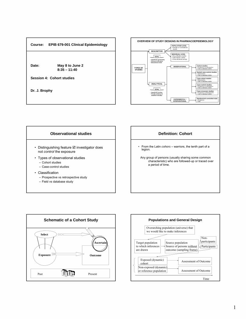
Observational studies
• Distinguishing feature investigator does not control the exposure
• Types of observational studies– Cohort studies– Case-control studies
• Classification– Prospective vs retrospective study– Field vs database study
Definition: Cohort
• From the Latin cohors – warriors, the tenth part of a legion.
Any group of persons (usually sharing some commoncharacteristic) who are followed-up or traced over a period of time.
Schematic of a Cohort Study
Exposure Outcome
Select
Ascertain
Past Present
Populations and General Design
Target populationto which inferencesare drawn
Source populationSource of persons withoutoutcome (sampling frame)
Exposed (dynamic)cohort
Non-exposed (dynamic)or reference population
Assessment of Outcome
Assessment of Outcome
Overarching population (universe) that we would like to make inferences
Time
Participants
Non-participants

2
Cohort studies
• Group that shares a common experience
• Subjects classified on the basis of exposure status
• Longitudinal studies followed for a specified period of time until events occur
• Distinguishing feature compare rates of events/outcomes by exposure group
Comparison
Cohort studies
• If rate of event among exposed > rate of event in unexposed = harmful drug
• If rate of event among exposed < rate of event in exposed = protective drug
Timing
Cohort design Cohort studies
• Strengths– Can study rare exposures
– Can study multiple outcomes
– Temporality is assured causality criteria
– Unbiased selection of comparator group
– Retrospective studies are relatively quick and inexpensive … caution re: bias

3
Cohort studies
• Limitations– Inefficient for rare events/diseases or outcomes
with long induction periods– If prospective expensive and time consuming
• Sources of bias– Non-participation (selection in)– Losses to follow-up (selection out)– Recall / interviewer bias if retrospective
Potential problems
Definition: Bias
• Bias: Deviation of results or inferences from the truth, or processes leading to such deviation.
1. Systematic variations of measurements from their true values (systematic error; antonym, validity)
2. Variations of statistics from their true values as a result of systematic variation of measurements, other flaws in data collection, or flaws in study design and analysis.
Antonym: Validity
Biases
• Misclassifcation• Selection (chanelling)• Losses to follow-up (correlated to exposure
and disease)• Effect of non-participation
Selection bias Confounding

4
Confounding bias
Intervention Outcome
Confounder
• Age• Sex• Stage of disease• Previous treatments• Genetics• Behaviour• Others
Channeling Effect (or Channeling Bias):
• The tendency of clinicians to prescribe treatment based on a patient’s prognosis. As a result of the behavior, comparisons between treated and untreated patients will yield a biased estimate of treatment effect.
Effect modification Key questions for a cohort study
Key questions for a cohort study Comparisons

5
Comparisons All patients & hip fractures
Restricted cohort
Key questions for a cohort study Strengths of cohort studies
• Useful if exposure is rare• Can examine multiple effects of a single
exposure• Can elucidate temporal relationship• If prospective, minimizes ascertainment bias• Allows direct measurement of disease
incidence in both exposed and non-exposed groups

6
Limitations of cohort studies
• Inefficient for rare diseases• Can be expensive and time consuming if
prospective• If retrospective, need reliable records• Validity affected by losses to follow-up
Cholera in London in the mid-1800s: John Snow and the Beginnings of Epidemiology
Miasmata Theory
• Thought that cholera was brought to Europe from India
• Prevailing theory in the 1880s: airbornepoison arising from unhealthy and unsanitary conditions (“miasmata”)– Miasma: noxious exhalations from putrescent
organic matter; poisonous effluvia or germs infecting the environment
Hypothesis
• Higher rates in the south because water companies drew water from the polluted Thames River
Snow’s Experimentum Crucis
1849 1854Relatively low rates of cholera in London
Water Supply from Polluted Thames River:Southwark & Vauxhall Co.Lambeth Co.
Natural experiment:In 1852, Lambeth changed its source to a less polluted part of The Thames 1854 epidemic: Snow determined no. of homes
served by each companyCollected death reports and classified deaths by water companyCalculated ratios of deaths to no. of homes, by water company
Epidemiology
• Unit of observation is mixed:1. Numerator - the individual: fact, date, cause of
death, and water companyWater company obtained from detailed inquiry ortest of water for concentrations of NaCl
2. Denominator – the number of homes (not individuals) served by each company
• Statistic: Ratio=Numerator/Denominator (unit: persons/homes)– not a proportion (unitless)
7
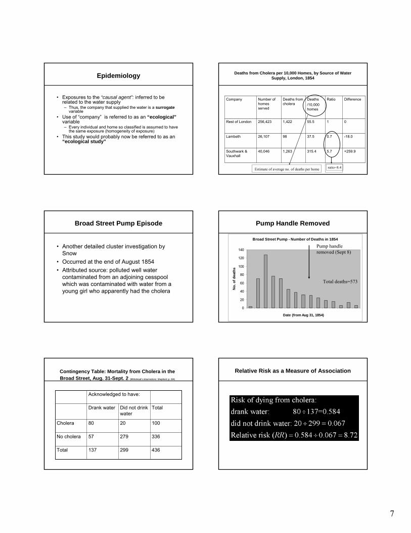
Epidemiology
• Exposures to the “causal agent”: inferred to be related to the water supply– Thus, the company that supplied the water is a surrogate
variable• Use of “company” is referred to as an “ecological”
variable– Every individual and home so classified is assumed to have
the same exposure (homogeneity of exposure)• This study would probably now be referred to as an
“ecological study”
Deaths from Cholera per 10,000 Homes, by Source of Water Supply, London, 1854
+259.9
-18.0
0
Difference
5.7315.41,26340,046Southwark & Vauxhall
0.737.59826,107Lambeth
155.51,422256,423Rest of London
RatioDeaths/10,000 homes
Deaths from cholera
Number of homes served
Company
Estimate of average no. of deaths per home ratio=8.4
Broad Street Pump Episode
• Another detailed cluster investigation by Snow
• Occurred at the end of August 1854• Attributed source: polluted well water
contaminated from an adjoining cesspool which was contaminated with water from a young girl who apparently had the cholera
Broad Street Pump - Number of Deaths in 1854
0
20
40
60
80
100
120
140
Date (from Aug 31, 1854)
No.
of d
eath
s
Pump handleremoved (Sept 8)
Total deaths=573
Pump Handle Removed
Contingency Table: Mortality from Cholera in the Broad Street, Aug. 31-Sept. 2 (Whitehead’s observations: Shephard, p. 224)
436299137Total
33627957No cholera
1002080Cholera
TotalDid not drink water
Drank water
Acknowledged to have:
Relative Risk as a Measure of Association
8
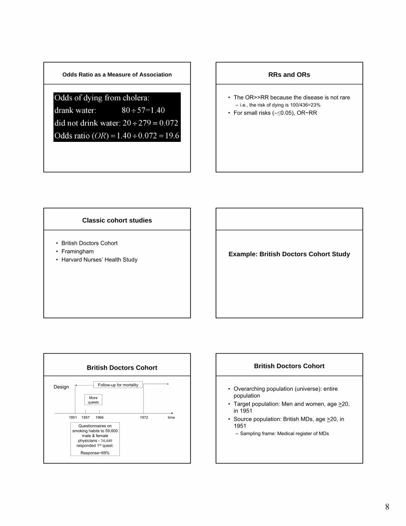
Odds Ratio as a Measure of Association RRs and ORs
• The OR>>RR because the disease is not rare– i.e., the risk of dying is 100/436=23%
• For small risks (∼≤0.05), OR~RR
Classic cohort studies
• British Doctors Cohort• Framingham• Harvard Nurses’ Health Study
Example: British Doctors Cohort Study
Design
1951 1957 1966 1972 time
More quests
Questionnaires on smoking habits to 59,600
male & femalephysicians - 34,440
responded 1st quest.
Response~69%
Follow-up for mortality
British Doctors Cohort British Doctors Cohort
• Overarching population (universe): entire population
• Target population: Men and women, age >20, in 1951
• Source population: British MDs, age >20, in 1951– Sampling frame: Medical register of MDs

9
British Doctors Cohort
• Exposure: Smoking information from subjectsbased on a short postal questionnaire– Current smokers
• Age started smoking• Amount consumed currently• Method of smoking
– Past smokers• Same as above• Date stopped smoking
– Never smoked regularly (<1 cigarette/year for one year)
British Doctors Cohort
• Outcome:– Mortality ascertained by looking-up death
certificates– Cause of death is filled in by a physician or the
coroner• Analysis:
– Compare rates of death according to level of self-reported smoking
Typical Questions about Smoking
• Type of smoking (cigarettes, cigars, pipes)• Have you ever smoked regularly?• How old were you when you started to smoke?• How many cigarettes per day do you smoke
now?• If you stopped completely, how long ago was
this?
Metrics of Exposure to Tobacco Smoke
• The following indices can be estimated:– Type of smoking (cigarettes, cigars, pipes)– Duration (time since starting)– Time since quiting– Average Intensity (e.g., no. of cigarettes/day)– Frequency (e.g., percent time smoked in a week)– Current smoking status
Metrics of Exposure
• Cumulative exposure: frequency of smoking x intensity x duration– E.g., 1 pack per day x 20 cigarettes/pack x 365
days/year x 30 years= 219,000 cigarette-days=30 pack-years
• Lagged cumulative exposure (e.g., excluding last 10 years of smoking)
Definitions: Exposure and Dose
• Exposure: The presence of a substance in the environment external to the subject (external/environmental)
• Dose: The amount of a substance that reaches susceptible targets in the body (internal)

10
British Doctors
• Amount smoked at time of administration of firstquestionnaire:
Non-smokersCurrent: 1-14 cigs/day
15-24 ≥ 25
• These groups represent sub-cohorts defined by exposure at time of entry into the study
• However, information obtained during follow-up can change exposure status, so these sub-cohorts would not be fixed
British Doctors Cohort: Men
NA
NA
NA
NA
18,963
40,637 (69%)
N/A
N/A
1st Quest
362445369Other
2240372Not found
1026336Refused
216531Too ill
5071156508Reasons for nonresponse
23,299 (97.9%)26,163 (96.4%)30,810 (98.4%)Replied
238062713931318Presumably alive
1063473013122Known to have died
4th Quest3rd Quest2nd QuestSurvey period
British Doctors Study: Lung Cancer in Men among Current Smokers from Data Obtained at Last
Questionnaire
25.1251>25
12.712715-24
7.8
8.2
5.8 (=58/10)
14 (=140/10)
1
Mortality Rate Ratio
781-14
Cigarettes only (No. per day)
82Mixed
58Pipe &/or cigars
140Cigarettes only
10Non smokers
Age-standardized death rate (10-5)
Nested Case-Control Studies
• Sub-study that is based on an explicit cohort• Motivation:
– Computational ease for large datasets– Require additional information not already
collected• To reduce costs, a sample of subjects from the original
cohort is taken
Synonyms
• Case-control-within-cohort studies• Incidence density sampling studies• Synthetic case-control studies
• Case-control studies are also referred to as case-referent studies
Incidence Density Sampling
0 1 2 3 4 5 6 7 8 9 10 11 12 13 14 15 16 Time
No.12345678
Time for 1st failure
Time for 2nd failureRisk set for 1st failure
Risk set for 2nd failure

11
Incidence Density Sampling
1. For each failure time (T) of each case, define all subjects who at that time are still at risk of developing the outcome
– The complete set of such subjects is called the risk set for the case
– Will exclude all subjects who before T were:• Censored• Failed
Incidence Density Sampling
2. Randomly select without replacement a sample of “controls” from the risk set
• These subjects are therefore “matched” to the case by time of event
• Other matching variables can be used so that the sampling is stratified; e.g., select only a random sample of women
• If a potential control eventually becomes a case, he is still at-risk at the time of the event
• A fixed number of controls can be selected; that number can vary from risk set to risk set
Incidence Density Sampling
3. The analysis of these data is similar to the stratified analysis used in the M-H procedure for rates
4. The strata are now defined as each selected risk set.
Incidence Density Sampling
5. The measure of association is the odds ratio. With this sampling strategy and a matched analysis, it provides an unbiased estimate of the rate ratio.
• A matched analysis is one that accounts explicitly for the matching during the fieldwork
Incidence Density Sampling
6. The estimated OR will have more variability than the full M-H cohort analysis because fewer subjects are included
7. There is no need to calculate person-years in this analysis. It is subsumed automatically in the sampling.
Incidence Density Sampling
8. Odds ratios in each risk set are not calculated; rather a summary estimate across all risk sets is obtained.
• This assumes that the rate ratio does not vary by time (proportional hazards assumption). Equivalently, the OR across strata (matched subjects) are ~ equal (homogeneous).
9. Only risk sets that are discordant on exposure contribute information

12
Examples
Background
• Stenting common Rx for CAD symptoms• Statin therapy improves survival in secondary
prevention in conservatively treated patients• Is the same benefit present following
stenting?
Methods
• 4,520 patients < 80• Examined 1 year mortality• 3,585 with statins on discharge• 935 no statins on discharge
Results
• Mortality 2.6% statins, 5.6% no statins• Unadjusted OR 0.46 (95% 0.33 – 0.65)• Adjusted OR 0.51 (95% 0.36 – 0.71)• Methods included propensity analysis for
statin prescription and Cox PH model with a substantial number of clinical covariates
NEJM 1998;339:1349-57
Typical RCT

13
So, what’s the problem?
51% reduction in mortality observed in 12 months
24% reduction in mortality observed in 72 months
Red Flag
• If it looks too good to be true, it probably is too good to be true
Potential Biases
• Channeling (selection bias in pharmacoepistudies)
• Misclassification (exposure is not time independent)
1 2 3 4 5 6 7 8 9 10 11 12
8
7
6
5
4
3
2
1
X
X
X
Time (Months)
Statin Group
No Statin Group
RR = 1/4 / 2/4 =.5
RR = 1/ 42 person-months / 2 /42 pm = 0.5
1 2 3 4 5 6 7 8 9 10 11 12
8
7
6
5
4
3
2
1
X
X
X
Time (Months)
Statin Group
No Statin Group
D/C @ 1 month - 11 months non-statin exposureX
Start statin @ 1 month - 6 months -statin exposureX
Person-time
Statin = 2 / 37 Non statin = 1 / 47
RR = 2.4
A different approach
Results: Decrease in mortality of 34% 95%CI (4-55%) after 36 months)
(Am Heart J 2005;150:282- 7.)

14
Message
• Vital to consider the time dependency of drug exposure
• Another relatively easy method is to perform a nested case control study that matches on cohort entry
• Assure equal follow-up time